Forest Height Estimation Based on P-Band Pol-InSAR Modeling and Multi-Baseline Inversion

Abstract

The Gaussian vertical backscatter (GVB) model has a pivotal role in describing the forest vertical structure more accurately, which is reflected by P-band polarimetric interferometric synthetic aperture radar (Pol-InSAR) with strong penetrability. The model uses a three-dimensional parameter space (forest height, Gaussian mean representing the strongest backscattered power elevation, and the corresponding standard deviation) to interpret the forest vertical structure. This paper establishes a two-dimensional GVB model by simplifying the three-dimensional one. Specifically, the two-dimensional GVB model includes the following three cases: the Gaussian mean is located at the bottom of the canopy, the Gaussian mean is located at the top of the canopy, as well as a constant volume profile. In the first two cases, only the forest height and the Gaussian standard deviation are variable. The above approximation operation generates a two-dimensional volume only coherence solution space on the complex plane. Based on the established two-dimensional GVB model, the three-baseline inversion is achieved without the null ground-to-volume ratio assumption. The proposed method improves the performance by 18.62% compared to the three-baseline Random Volume over Ground (RVoG) model inversion. In particular, in the area where the radar incidence angle is less than 0.6 rad, the proposed method improves the inversion accuracy by 34.71%. It suggests that the two-dimensional GVB model reduces the GVB model complexity while maintaining a strong description ability.

1. Introduction

The essence of the model-based polarimetric interferometric synthetic aperture radar (Pol-InSAR) parameter inversion is to solve the model equations established between the synthetic aperture radar (SAR) observations and the theoretical forest vertical structure [1,2,3,4,5,6,7]. The Random Volume over Ground (RVoG) model based on the assumption of vertical homogeneous random volume was widely verified at relatively high frequencies (e.g., X-, C- and L-band) [5,6,7,8,9,10,11,12,13,14].

In the process of the Pol-InSAR model inversion, a non-negligible issue is whether the equations has a unique solution. An effective precondition for single-baseline Quad-pol configuration to make the RVoG model solution unique is the null ground-to-volume ratio assumption (commonly less than −10 dB) [6]. Nevertheless, this assumption is no longer valid for P-band observations in which all polarization channels generally contain significant ground responses [15,16,17,18,19].

A common solution to this case is to fix the extinction coefficient in the RVoG model [15,16,20,21,22]. However, as the inversion performance depends heavily on the selection of extinction coefficient, this technique is restricted in complex actual scene, in which it is unreasonable to apply only a single extinction coefficient to the parameter estimation of whole scene. An alternative is to increase the observation space through the multi-baseline configuration [8,17,23,24,25,26], and yet in this case, the inversion based on RVoG model is still obviously underestimated, indicating that multi-baseline is not enough to make up for the lack of the RVoG model [17,23]. Actually, when P-band SAR systems are used to observe the low-density forest, the volume scattering layer exhibits a vertical heterogeneous distribution, leading to the ineffectiveness of RVoG model [17].

To cope with this issue, the Gaussian vertical backscatter (GVB) model with a stronger expression ability was proposed [27,28]. The GVB model is mainly used to describe the vertical heterogeneity of volume scattering, which is often effective for the Pol-InSAR inversion where most backscatters are concentrated in the middle or lower part of the canopy. Compared with the RVoG model which has only two parameters (forest height and extinction coefficient), the GVB model describes the forest vertical structure with three parameters (forest height, Gaussian mean and standard deviation), which effectively improves the description ability of the model, yet brings serious inversion complexity simultaneously [24,25].

In view of the characteristics of P-band Pol-InSAR observations and the limitations of the existing methods, this paper proposes the two-dimensional GVB model and the corresponding multi-baseline inversion. Concretely, in order to apply to the heterogeneity of the forest vertical volume under P-band observations, the GVB model framework is used to interpret the forest vertical structure. Concurrently, to alleviate the high complexity of the three-dimensional GVB model, the two-dimensional GVB model is developed. As for the the model inversion, considering the assumption of null ground-to-volume ratio is no longer tenable, the multi-baseline configuration is adoped to optimize the model equations.

The remaining part of the paper proceeds as follows. Section 2 retrospects the model-based Pol-InSAR inversion theory. Section 3 presents the inversion based on the two-dimensional GVB model, while Section 4 validates the proposed approach with the actual E-SAR data. Finally, the discussions and conclusions are drawn in Section 5.

2. Model-Based Pol-InSAR Inversion Theory

Once temporal decorrelation and noise decorrelation are ignored, the interferometric coherence in Pol-InSAR observation mainly includes the volume decorrelation [5,6,7,29,30]

$$\begin{array}{c}\hfill \gamma =\frac{{\int }_{z_0}^{z_0+h_v}F\left(z\right)e^{j{k}_{z}z}dz}{{\int }_{z_0}^{z_0+h_v}F\left(z\right)dz}\end{array}$$

(1)

where $F\left(z\right)$ is the structure function related to the vertical coordinate z, $h_v$ and $z_0$ refer to the forest height and the ground starting coordinate respectively. The interferometric vertical wavenumber $k_z$ is related to the radar wavelength $\lambda$, incidence angle $\theta$ and the incidence angle difference between two interferometric antennas $\delta \theta$ [31]

$$\begin{array}{c}\hfill k_z=\frac{4\pi }{\lambda sin\theta }\delta \theta \end{array}$$

(2)

2.1. RVoG Model and Inversion

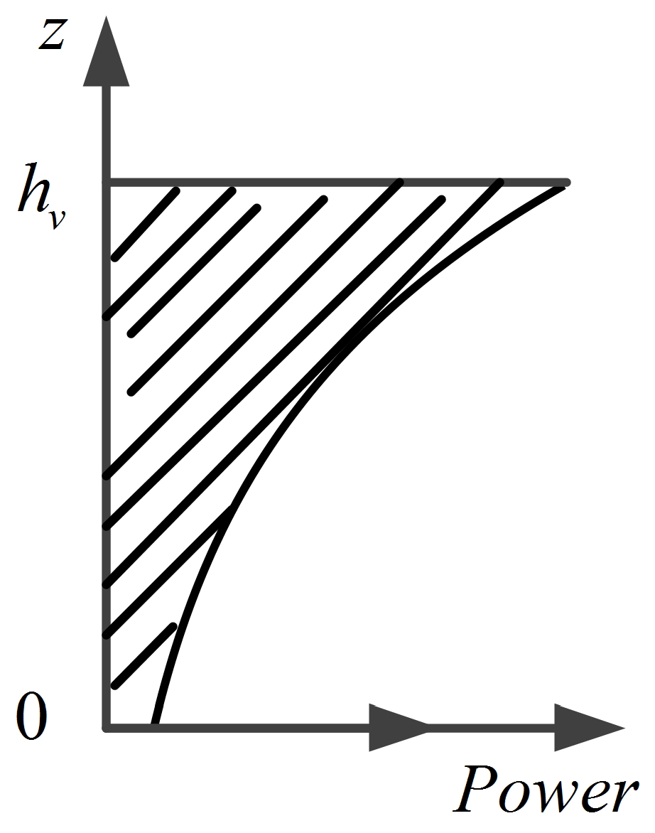
As shown in Figure 1, the vertical structure function based on the RVoG model is given [6,7,29,30,32]

$$\begin{array}{c}\hfill F\left(z\right)={\rho }_v{e}^{\left(2\sigma \left(z-z_0-h_v\right)/cos\theta \right)}+{\rho }_g{e}^{\left(-2\sigma h_v/cos\theta \right)}\delta \left(z-z_0\right)\end{array}$$

(3)

where $\sigma$ indicates the extinction coefficient independent of polarization, $\delta \left(•\right)$ refers to the impulse function, ${\rho }_v$ and ${\rho }_g$ related to the specific polarization state represent the backscatter intensities per unit length corresponding to the volume and ground, respectively.

Substituting Equation (3) into Equation (1) gives the volume decorrelation under the assumption of the RVoG model

$$\begin{array}{c}\hfill \gamma \left(\mathit{\omega }\right)=e^{j{\varphi }_0}\frac{{\gamma }_v+\mu \left(\mathit{\omega }\right)}{1+\mu \left(\mathit{\omega }\right)}\end{array}$$

(4)

where ${\varphi }_0=k_z{z}_0$ is the ground interferometric phase, $\mathit{\omega }$ represents the unit vector characterizing polarization, ${\gamma }_v$ and $\mu \left(\mathit{\omega }\right)$ indicate the volume only coherence and the ground-to-volume power ratio [6,7,29,30,32]

$$\begin{array}{c}\hfill {\gamma }_v\left(h_v,\sigma \right)=\frac{{\int }_0^{h_v}{e}^{\left(2\sigma z/cos\theta \right)}{e}^{j{k}_{z}z}dz}{{\int }_0^{h_v}{e}^{\left(2\sigma z/cos\theta \right)}dz}=\frac{2\sigma }{cos\theta \left(e^{\left(2\sigma h_v/cos\theta \right)}-1\right)}{\int }_0^{h_v}{e}^{\left(2\sigma z/cos\theta \right)}{e}^{j{k}_{z}z}dz\end{array}$$

(5)

$$\begin{array}{c}\hfill \mu \left(\mathit{\omega }\right)=\frac{2\sigma }{cos\theta \left(e^{\left(2\sigma h_v/cos\theta \right)}-1\right)}\frac{{\rho }_g}{{\rho }_v}\end{array}$$

(6)

According to the random volume hypothesis, the extinction coefficient $\sigma$ is independent of polarization, while ${\varphi }_0$ depends on the baseline. Therefore, once the baseline is determined, $h_v$, $\sigma$ and ${\varphi }_0$ in Equations (4) and (5) remain unchanged, while only $\mu \left(\mathit{\omega }\right)$ varies with polarization state. Since the single-baseline Quad-pol provides three measured complex coherences corresponding to independent polarization channels, the parameter inversion can be achieved by a six-dimensional optimization process [5,6,15,17,19]

$$\begin{array}{c}\hfill {\left[\begin{array}{cccc}{\widehat{h}}_v,& \widehat{\sigma },& {\widehat{\varphi }}_0,& {\widehat{\mu }}_i\end{array}\right]}^T=\underset{\left[h_v,\sigma ,{\varphi }_0,{\mu }_i\right]}{\mathrm{a}rgmin} \left\{∥\left[\begin{array}{c}\widehat{\gamma }\left({\mathit{\omega }}_1\right)\\ \widehat{\gamma }\left({\mathit{\omega }}_2\right)\\ \widehat{\gamma }\left({\mathit{\omega }}_3\right)\end{array}\right]-\left[\begin{array}{c}\gamma \left(h_v,\sigma ,{\varphi }_0,{\mu }_1\right)\\ \gamma \left(h_v,\sigma ,{\varphi }_0,{\mu }_2\right)\\ \gamma \left(h_v,\sigma ,{\varphi }_0,{\mu }_3\right)\end{array}\right]∥\right\}\end{array}$$

(7)

where ${\left[\begin{array}{cccc}{\widehat{h}}_v,& \widehat{\sigma },& {\widehat{\varphi }}_0,& {\widehat{\mu }}_i\end{array}\right]}^T$ is the parameter estimation and subscript $i=1,2,3$ represent any three independent polarization channels. $∥•∥$ denotes the matrix 2-norm operation, $\widehat{\gamma }$ and $\gamma$ represent the radar observation and the theoretical prediction respectively. Although the optimization process consists of six unknowns and six independent equations, the inversion cannot get a unique solution due to the nonlinear form of the equation [17].

One way to guarantee a unique solution to the single-baseline configuration is to assume that there is at least one polarization channel with little ground response [6,7,17]. Under this assumption, ${\mu }_3=0$ can be set directly, and the optimization expression at this time is as follows

$$\begin{array}{c}\hfill {\left[\begin{array}{cccc}{\widehat{h}}_v,& \widehat{\sigma },& {\widehat{\varphi }}_0,& {\widehat{\mu }}_i\end{array}\right]}^T=\underset{\left[h_v,\sigma ,{\varphi }_0,{\mu }_i\right]}{\mathrm{a}rgmin} \left\{∥\left[\begin{array}{c}\widehat{\gamma }\left({\mathit{\omega }}_1\right)\\ \widehat{\gamma }\left({\mathit{\omega }}_2\right)\\ \widehat{\gamma }\left({\mathit{\omega }}_3\right)\end{array}\right]-\left[\begin{array}{c}\gamma \left(h_v,\sigma ,{\varphi }_0,{\mu }_1\right)\\ \gamma \left(h_v,\sigma ,{\varphi }_0,{\mu }_2\right)\\ \gamma \left(h_v,\sigma ,{\varphi }_0,{\mu }_3=0\right)\end{array}\right]∥\right\}\end{array}$$

(8)

As mentioned before, the null ground-to-volume ratio assumption is no longer effective for P-band SAR observations. In this case, a common single-baseline inversion method for P-band observations is to fix the extinction coefficient [15,16,20,21,22]

$$\begin{array}{c}\hfill {\left[\begin{array}{ccc}{\widehat{h}}_v,& {\widehat{\varphi }}_0,& {\widehat{\mu }}_i\end{array}\right]}^T=\underset{\left[h_v,{\varphi }_0,{\mu }_i\right]}{\mathrm{a}rgmin} \left\{∥\left[\begin{array}{c}\widehat{\gamma }\left({\mathit{\omega }}_1\right)\\ \widehat{\gamma }\left({\mathit{\omega }}_2\right)\\ \widehat{\gamma }\left({\mathit{\omega }}_3\right)\end{array}\right]-\left[\begin{array}{c}\gamma \left(h_v,\sigma ={\sigma }_{pre},{\varphi }_0,{\mu }_1\right)\\ \gamma \left(h_v,\sigma ={\sigma }_{pre},{\varphi }_0,{\mu }_2\right)\\ \gamma \left(h_v,\sigma ={\sigma }_{pre},{\varphi }_0,{\mu }_3\right)\end{array}\right]∥\right\}\end{array}$$

(9)

where ${\sigma }_{pre}$ represents the extinction coefficient that is determined by prior or empirical information.

Another method to ensure that the inversion has a unique solution while not requiring the null ground-to-volume ratio assumption is the multi-baseline optimization [17,23]

$$\begin{array}{c}\hfill {\left[\begin{array}{cccc}{\widehat{h}}_v,& \widehat{\sigma },& {\widehat{\varphi }}_0^j,& {\widehat{\mu }}_i\end{array}\right]}^T=\underset{\left[h_v,\sigma ,{\varphi }_0^j,{\mu }_i\right]}{\mathrm{a}rgmin} \left\{∥\left[\begin{array}{c}{\widehat{\gamma }}^1\left({\mathit{\omega }}_1\right)\\ {\widehat{\gamma }}^1\left({\mathit{\omega }}_2\right)\\ {\widehat{\gamma }}^1\left({\mathit{\omega }}_3\right)\\ \dots \\ {\widehat{\gamma }}^n\left({\mathit{\omega }}_1\right)\\ {\widehat{\gamma }}^n\left({\mathit{\omega }}_2\right)\\ {\widehat{\gamma }}^n\left({\mathit{\omega }}_3\right)\end{array}\right]-\left[\begin{array}{c}{\gamma }^1\left(h_v,\sigma ,{\varphi }_0^1,{\mu }_1\right)\\ {\gamma }^1\left(h_v,\sigma ,{\varphi }_0^1,{\mu }_2\right)\\ {\gamma }^1\left(h_v,\sigma ,{\varphi }_0^1,{\mu }_3\right)\\ \dots \\ {\gamma }^n\left(h_v,\sigma ,{\varphi }_0^n,{\mu }_1\right)\\ {\gamma }^n\left(h_v,\sigma ,{\varphi }_0^n,{\mu }_2\right)\\ {\gamma }^n\left(h_v,\sigma ,{\varphi }_0^n,{\mu }_3\right)\end{array}\right]∥\right\}\end{array}$$

(10)

where the superscript $j=1,2,\dots ,n$ represent different baselines, among which n is the total number of baselines involved in the optimization. Under similar experimental environments (radar system parameters, weather conditions, etc.), ${\mu }_i$ of different interferometric pairs are assumed to be constant in the same polarization [24,25,33]. Consequently, for each additional interferometric pair, the corresponding optimization increases three observational complex coherences and produces an unknown variable ${\varphi }_0$ simultaneously. In other words, when n interferometric pairs are involved in inversion, the optimization process includes $6n$ independent equations and $n+5$ unknowns concurrently.

2.2. GVB Model and Inversion

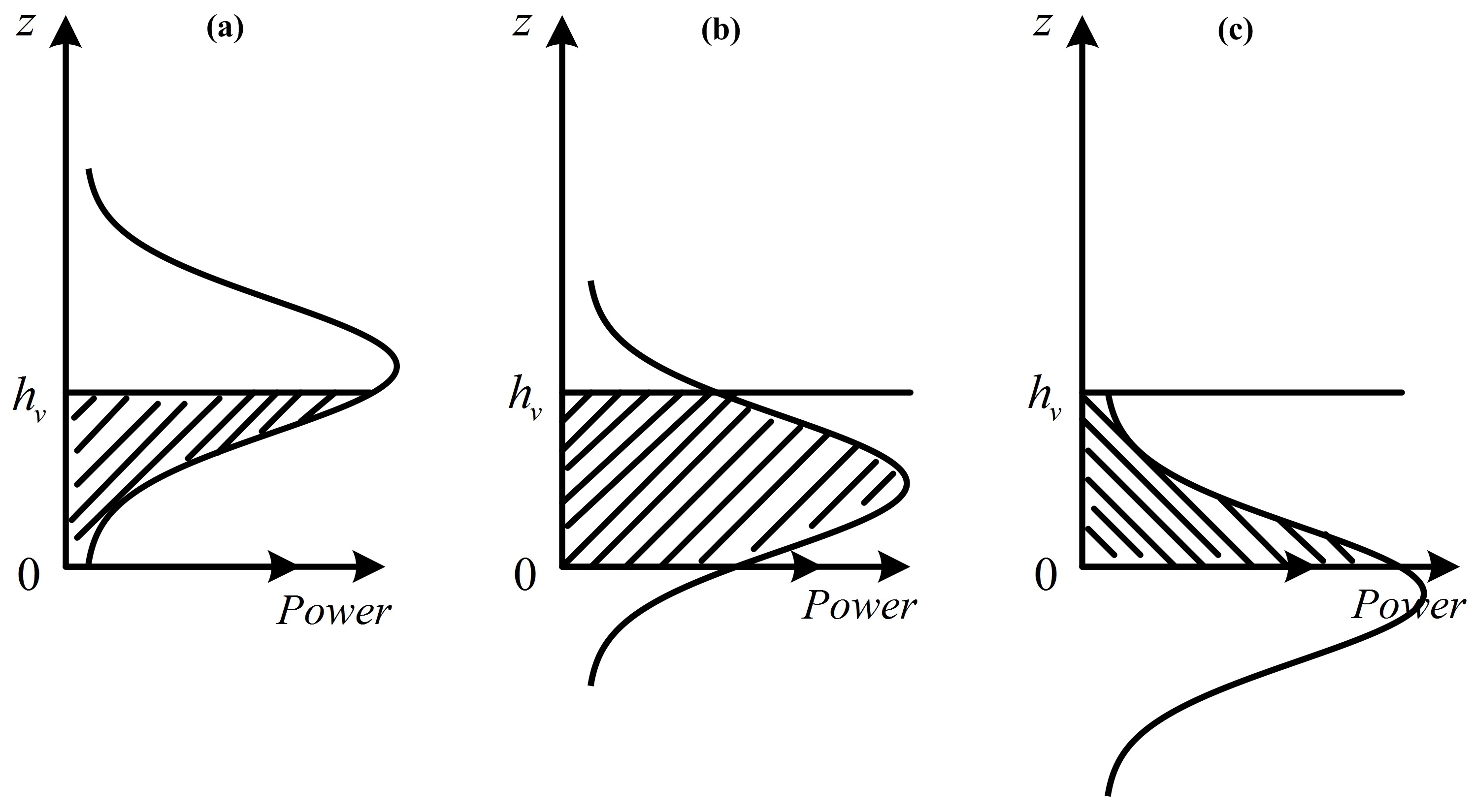
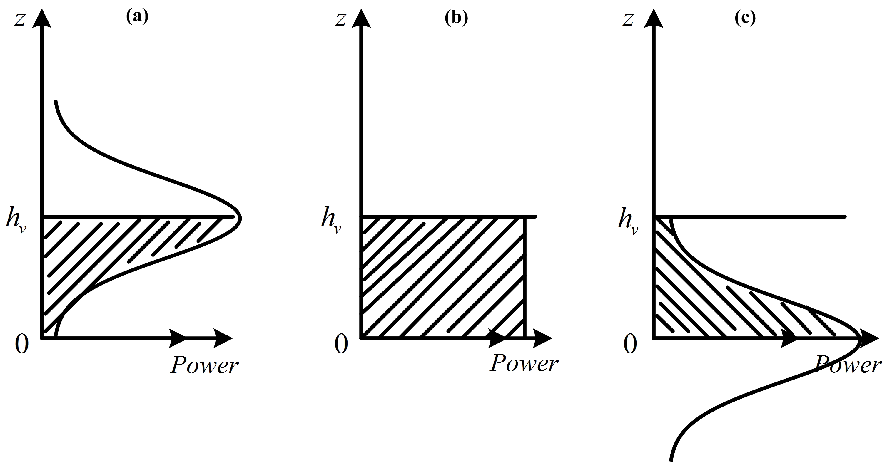
As presented in Figure 2, the GVB model can be divided into three situations in line with the position of $\delta$. The first case in Figure 2a is similar to the RVoG model, which assumes that the strongest backscatter power is located at the top of the canopy, while Figure 2b,c are supplements of GVB model for the heterogeneity of the canopy under P-band observations [25]. The volume only coherence based on the GVB model is [27,28]

$$\begin{array}{c}\hfill {\gamma }_v\left(h_v,\delta ,\chi \right)=\frac{{\int }_0^{h_v}{e}^{-\frac{{\left(z-\delta \right)}^2}{2{\chi }^2}+j{k}_{z}z}dz}{{\int }_0^{h_v}{e}^{-\frac{{\left(z-\delta \right)}^2}{2{\chi }^2}}dz}=e^{-\frac{{\chi }^2{k}_z^2}{2}+j\delta k_z}\frac{erf\left(\frac{1}{\sqrt{2}}\left(j\chi k_z+\frac{\delta }{\chi }\right)\right)-erf\left(\frac{1}{\sqrt{2}}\left(j\chi k_z+\frac{\delta -h_v}{\chi }\right)\right)}{erf\left(\frac{h_v-\delta }{\sqrt{2}\chi }\right)+erf\left(\frac{\delta }{\sqrt{2}\chi }\right)}\end{array}$$

(11)

where $\delta$ and $\chi$ represent the backscatter mean elevation and the corresponding standard deviation respectively, and $\mathrm{erf}\left(•\right)$ indicates the error function.

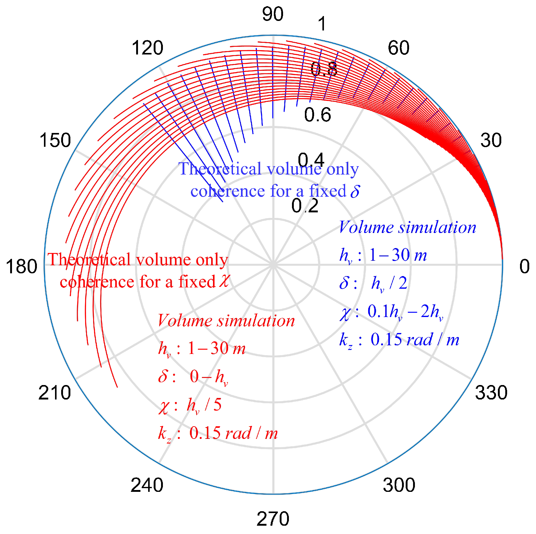
When $\delta$ or $\chi$ is fixed, the corresponding solution spaces of GVB model are shown in Figure 3, from which it can be found that there is an overlapping area between the two solution spaces. It illustrates that once $\delta$ and $\chi$ both can take arbitrary values, there are some identical elements in the corresponding three-dimensional volume only coherence solution space. This will lead to multiple solutions [24,25].

Under the assumption of the two-layer volume over ground model, the interferometric coherence based on the GVB model also conforms to Equation (4). As more model parameters are included as well as the Gaussian form of vertical structure function (resulting in multiple solutions as presented in Figure 3), the GVB model inversion theoretically requires multi-baseline observations to ensure that the forest vertical structure with reasonable physical significance can be obtained [24,25]

$$\begin{array}{c}\hfill {\left[\begin{array}{ccccc}{\widehat{h}}_v,& \widehat{\delta },& \widehat{\chi },& {\widehat{\varphi }}_0^j,& {\widehat{\mu }}_i\end{array}\right]}^T=\underset{\left[h_v,\delta ,\chi ,{\varphi }_0^j,{\mu }_i\right]}{\mathrm{a}rgmin} \left\{∥\left[\begin{array}{c}{\widehat{\gamma }}^1\left({\mathit{\omega }}_1\right)\\ {\widehat{\gamma }}^1\left({\mathit{\omega }}_2\right)\\ {\widehat{\gamma }}^1\left({\mathit{\omega }}_3\right)\\ \dots \\ {\widehat{\gamma }}^n\left({\mathit{\omega }}_1\right)\\ {\widehat{\gamma }}^n\left({\mathit{\omega }}_2\right)\\ {\widehat{\gamma }}^n\left({\mathit{\omega }}_3\right)\end{array}\right]-\left[\begin{array}{c}{\gamma }^1\left(h_v,\delta ,\chi ,{\varphi }_0^1,{\mu }_1\right)\\ {\gamma }^1\left(h_v,\delta ,\chi ,{\varphi }_0^1,{\mu }_2\right)\\ {\gamma }^1\left(h_v,\delta ,\chi ,{\varphi }_0^1,{\mu }_3\right)\\ \dots \\ {\gamma }^n\left(h_v,\delta ,\chi ,{\varphi }_0^n,{\mu }_1\right)\\ {\gamma }^n\left(h_v,\delta ,\chi ,{\varphi }_0^n,{\mu }_2\right)\\ {\gamma }^n\left(h_v,\delta ,\chi ,{\varphi }_0^n,{\mu }_3\right)\end{array}\right]∥\right\}\end{array}$$

(12)

where ${\left[\begin{array}{ccccc}{\widehat{h}}_v,& \widehat{\delta },& \widehat{\chi },& {\widehat{\varphi }}_0^j,& {\widehat{\mu }}_i\end{array}\right]}^T$ is the the parameter estimation. Similarly, it is assumed that $\delta$ and $\chi$ are independent of baseline and polarization. When n interferometric pairs are involved in inversion, the optimization process will include $6n$ independent equations and $n+6$ unknowns concurrently. In addition, in order to ensure the physical significance of parameter estimation, some prior or empirical knowledge can be used to calibrate the initial values and constraints in the optimization Equation (12) [24,25].

3. Two-Dimensional GVB Model and Inversion

3.1. Two-Dimensional GVB Model

Corresponding to the three cases in Figure 2, the two-dimensional GVB model is constructed by simplifying the original three-dimensional GVB model, as illustrated in Figure 4. Cases $\delta \ge h_v$ and $\delta \le 0$ are approximated to $\delta =h_v$ and $\delta =0$ respectively, while case $\delta \in \left(0, h_v\right)$ is approximated to a constant volume profile. In these three cases, $h_v$ and $\chi$ are varied, while $\delta$ remains stationary. Since the constant profile is equivalent to the case that $\chi$ is infinite when $\delta =h_v$ or $\delta =0$, only the following two cases are considered in the modeling of volume only coherence

$$\begin{array}{c}\hfill {\gamma }_v\left(h_v,\delta ,\chi \right){|}_{\delta =0}=\frac{{\int }_0^{h_v}{e}^{-\frac{z^2}{2{\chi }^2}+j{k}_{z}z}dz}{{\int }_0^{h_v}{e}^{-\frac{z^2}{2{\chi }^2}}dz}=e^{-\frac{{\chi }^2{k_z}^2}{2}}\frac{erf\left(\frac{1}{\sqrt{2}}j\chi k_z\right)-erf\left(\frac{1}{\sqrt{2}}\left(j\chi k_z-\frac{h_v}{\chi }\right)\right)}{erf\left(\frac{h_v}{\sqrt{2}\chi }\right)}\end{array}$$

(13)

$$\begin{array}{c}\hfill {\gamma }_v\left(h_v,\delta ,\chi \right){|}_{\delta =h_v}=\frac{{\int }_0^{h_v}{e}^{-\frac{{\left(z-h_v\right)}^2}{2{\chi }^2}+j{k}_{z}z}dz}{{\int }_0^{h_v}{e}^{-\frac{{\left(z-h_v\right)}^2}{2{\chi }^2}}dz}=e^{-\frac{{\chi }^2{k_z}^2}{2}+j{h}_v{k}_z}\frac{erf\left(\frac{1}{\sqrt{2}}\left(j\chi k_z+\frac{h_v}{\chi }\right)\right)-erf\left(\frac{1}{\sqrt{2}}j\chi k_z\right)}{erf\left(\frac{h_v}{\sqrt{2}\chi }\right)}\end{array}$$

(14)

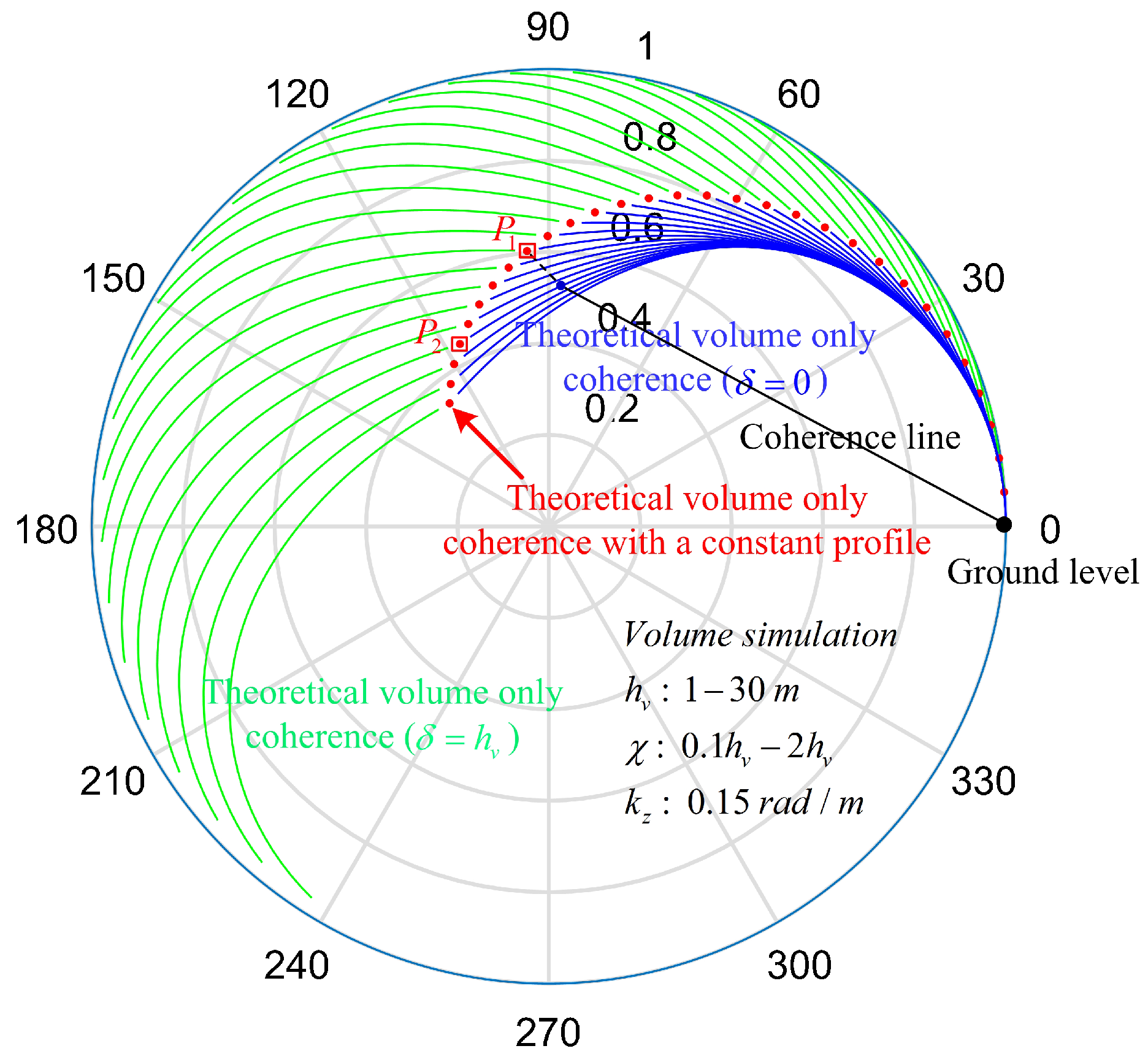
In line with Equations (13) and (14), the solution space of the two-dimensional GVB model ${\gamma }_v\left(h_v,\delta =0/h_v,\chi \right)$ on the complex plane can be drawn, as shown in Figure 5. Although $\delta$ may be 0 or $h_v$, the two cases correspond to two completely non-overlapping regions (blue and green solution spaces in Figure 5, respectively) on the complex plane. According to the setting of volume simulation parameters, with the same constant profile, the forest height corresponding to $P_1$ is smaller than that corresponding to $P_2$. Simultaneously, it can be seen that the solution volume only coherence and $P_2$ are on the same forest height curve. Hence, when the solution volume only coherence lies in the blue solution space, the solution space containing only $\delta =h_v$ will cause underestimation, which can be ameliorated by $\delta =0$ solution space. Since the null extinction (the extinction coefficient is zero) in RVoG model has the same solution space curve as the constant profile of the two-dimensional GVB model, and considering that the vertical structure described in Figure 1 and Figure 4a are similar, the solution space of RVoG model can be approximately equivalent to the case of $\delta =h_v$ in two-dimensional GVB model. In a word, the added $\delta =0$ solution space is the reason the two-dimensional GVB model is superior to the RVoG model [25].

In accordance with Figure 5, the solution space relying on the two-dimensional GVB model is a two-dimensional complex space. Therefore, each element in the solution space can be uniquely identified

$$\begin{array}{c}\hfill {\gamma }_v\left(h_v,\delta =0/h_v,\chi \right)={{\gamma }_v}^{re}+j{{\gamma }_v}^{im}\end{array}$$

(15)

where ${{\gamma }_v}^{re}$ and ${{\gamma }_v}^{im}$ are the real part and the imaginary part of the homologous volume only coherence, respectively.

In line with Figure 4 and Figure 5 and Equations (13) and (14), the solution spaces of $\delta =h_v$ and $\delta =0$ are not overlapped, so $\left(\delta =0/h_v, \chi \right)$ can be marked with a factor $\eta \left(\delta =0/h_v, \chi \right)$. The physical meaning of $\left(h_v,\eta \right)$ represents the vertical structure profile with a unique volume only coherence. In this case, Equation (15) can be rewritten as

$$\begin{array}{c}\hfill {\gamma }_v\left(h_v,\eta \right)={{\gamma }_v}^{re}+j{{\gamma }_v}^{im}\end{array}$$

(16)

where $\eta$ can be any marking mode in engineering implementation.

3.2. Pol-InSAR Inversion Based on Two-Dimensional GVB Model

The inversion conditions of the two-dimensional GVB volume over ground model and the two-parameter ($h_v$ and $\sigma$) RVoG model are the same, i.e., single-baseline Quad-pol configuration constructs six independent equations and six unknowns simultaneously. Therefore, in order to ensure a unique solution and avoid the null ground-to-volume ratio assumption, the multi-baseline configuration is used to carry out the two-dimensional GVB model inversion

$$\begin{array}{c}\hfill {\left[\begin{array}{cccc}{\widehat{h}}_v,& \widehat{\eta },& {\widehat{\varphi }}_0^j,& {\widehat{\mu }}_i\end{array}\right]}^T=\underset{\left[h_v,\eta ,{\varphi }_0^j,{\mu }_i\right]}{\mathrm{a}rgmin} \left\{∥\left[\begin{array}{c}{\widehat{\gamma }}^1\left({\mathit{\omega }}_1\right)\\ {\widehat{\gamma }}^1\left({\mathit{\omega }}_2\right)\\ {\widehat{\gamma }}^1\left({\mathit{\omega }}_3\right)\\ \dots \\ {\widehat{\gamma }}^n\left({\mathit{\omega }}_1\right)\\ {\widehat{\gamma }}^n\left({\mathit{\omega }}_2\right)\\ {\widehat{\gamma }}^n\left({\mathit{\omega }}_3\right)\end{array}\right]-\left[\begin{array}{c}{\gamma }^1\left(h_v,\eta ,{\varphi }_0^1,{\mu }_1\right)\\ {\gamma }^1\left(h_v,\eta ,{\varphi }_0^1,{\mu }_2\right)\\ {\gamma }^1\left(h_v,\eta ,{\varphi }_0^1,{\mu }_3\right)\\ \dots \\ {\gamma }^n\left(h_v,\eta ,{\varphi }_0^n,{\mu }_1\right)\\ {\gamma }^n\left(h_v,\eta ,{\varphi }_0^n,{\mu }_2\right)\\ {\gamma }^n\left(h_v,\eta ,{\varphi }_0^n,{\mu }_3\right)\end{array}\right]∥\right\}\end{array}$$

(17)

where ${\left[\begin{array}{cccc}{\widehat{h}}_v,& \widehat{\eta },& {\widehat{\varphi }}_0^j,& {\widehat{\mu }}_i\end{array}\right]}^T$ is the parameter estimation. Please note that since $\delta$ and $\chi$ are assumed to be independent of baseline and polarization, the factor $\eta$ is also independent of these two system observation variables. In Equation (17), n baselines can provide $6n$ independent equations, while there are $n+5$ unknowns to be solved.

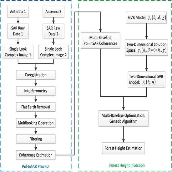
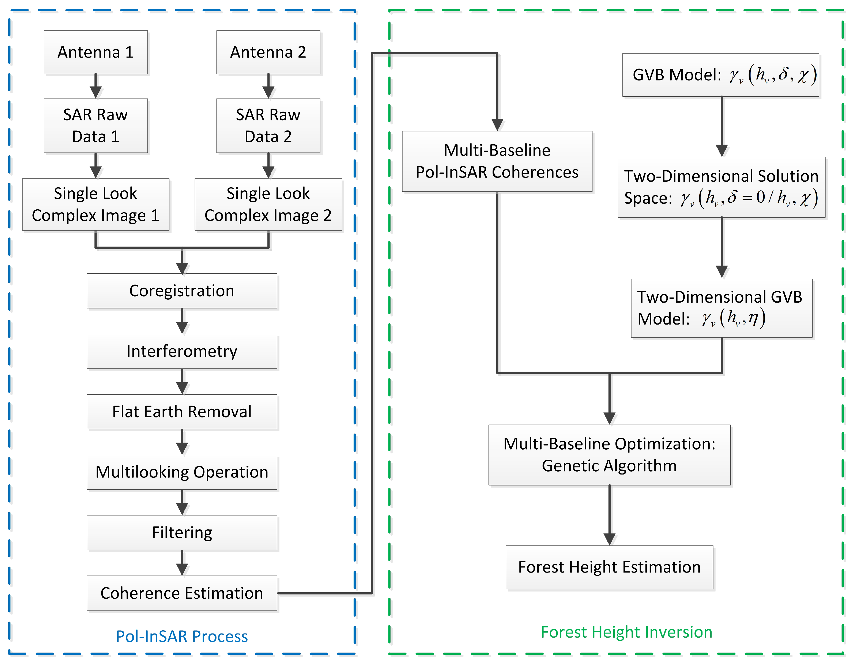
Figure 6 presents the flowchart of the proposed two-dimensional GVB modeling and multi-baseline inversion. The flowchart begins by the conventional Pol-InSAR processing (including imaging, coregistration, interferometry, flat earth removal, multilooking, filtering and coherence estimation). It then goes on to the modeling of the two-dimensional GVB model and the corresponding multi-baseline inversion, which is also the primary contribution made by this paper. First of all, the original three-dimensional GVB model is approximate to the two-dimensional GVB model. Although $\delta$ in two-dimensional GVB model still exists two possible values (0 or $h_v$), these two situations constitute a two-dimensional solution space of the new model without overlapping. Therefore, two parameters ($h_v$ and $\eta$ in Equation (16)) can be used to mark every possible volume only coherence in the solution space. In model inversion stage, the solution space corresponding to each baseline is different, which is related to the interferometric vertical wavenumber $k_z$, while $\left(h_v, \delta =0/h_v, \chi \right)$ is independent of the baseline. Therefore, in line with the one-to-one mapping relationship between $\left(h_v,\eta \right)$ and $\left(h_v, \delta =0/h_v, \chi \right)$, forest vertical structure estimates are ultimately available by using the genetic algorithm to optimize the inversion consisting of no less than two baselines [17].

4. Validation with P-Band Pol-InSAR Data

4.1. BIOSAR 2008 Data Introduction

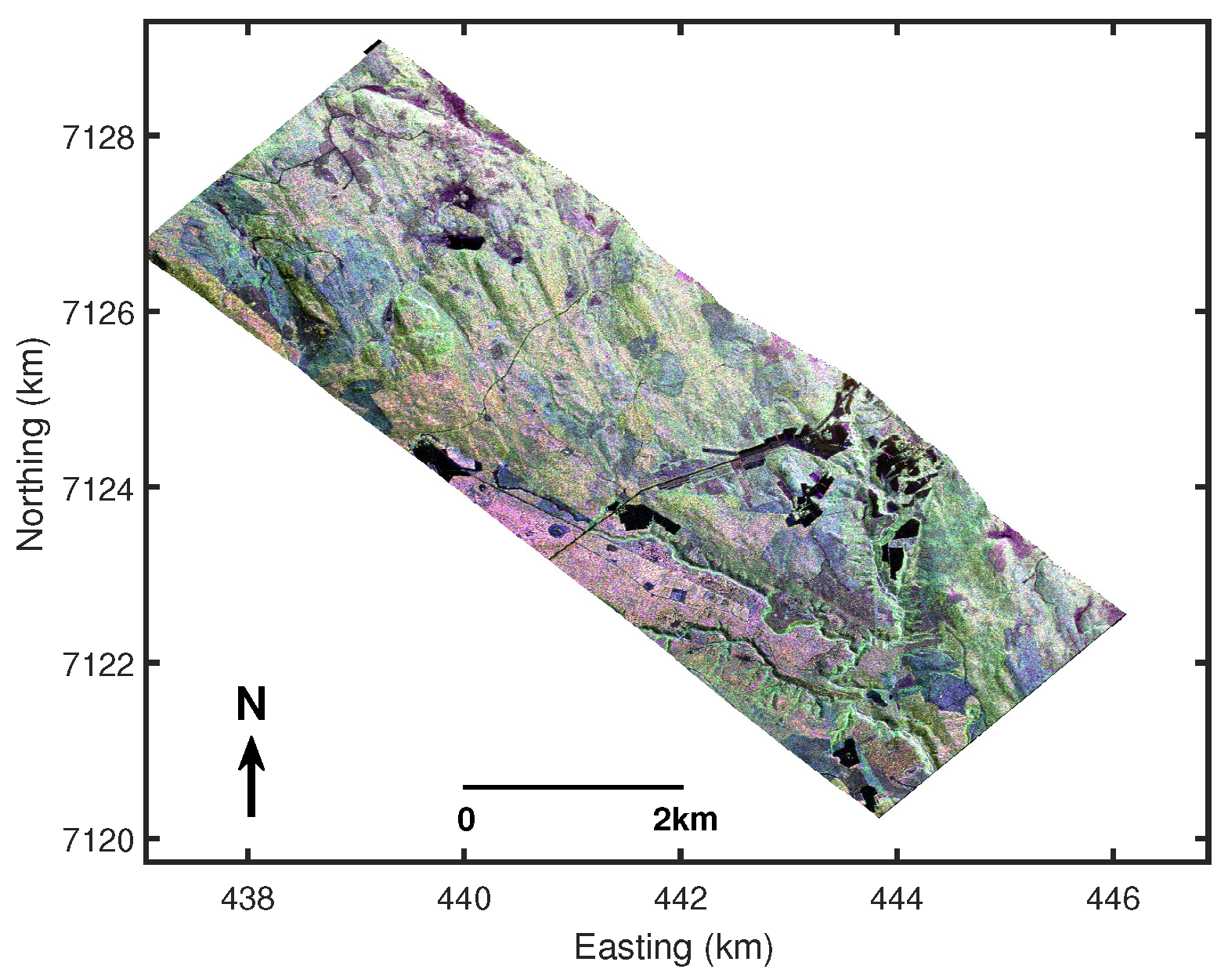
The data set applied in this paper is from European Space Agency (ESA) BIOSAR 2008 campaign, under which the P-band Pol-InSAR experiment was conducted by German Aerospace Center (DLR) E-SAR system. The experimental site is located in Krycklan catchment, Northern Sweden, mainly covered by boreal forest (spruce, pine, and birch), and the Pauli-basis polarization composite map is presented in Figure 7 [23]. On account of the significant topographic fluctuations in the test area, the external Digital Elevation Model (DEM) data is used to generate terrain slope to compensate the inversion model, without which there would be a certain degree of inversion error [23,26,29,30,34,35,36,37]. In addition, the LiDAR-measured forest height provided in the data set is used as the true value to evaluate the inversion performance. To carry out the multi-baseline optimization, three interferometric pairs with baseline lengths of 16 m, 24 m and 32 m are selected in this paper, and the corresponding parameter information is illustrated in

Table 1. Pol-InSAR data parameters.

Track	Baseline (m)	${\mathit{k}}_{\mathit{z}}$ Range (rad/m)	$\mathit{\theta }$ Range (rad)	Band	Polarization
Master	Master	Master	0.44–0.96	P	Quad
Slave	16	0.014–0.135	Slave	P	Quad
Slave	24	0.021–0.181	Slave	P	Quad
Slave	32	0.026–0.245	Slave	P	Quad

. Please note that the incidence angle range in Table 1 is not corrected for terrain slope.

4.2. Experimental Results and Analysis

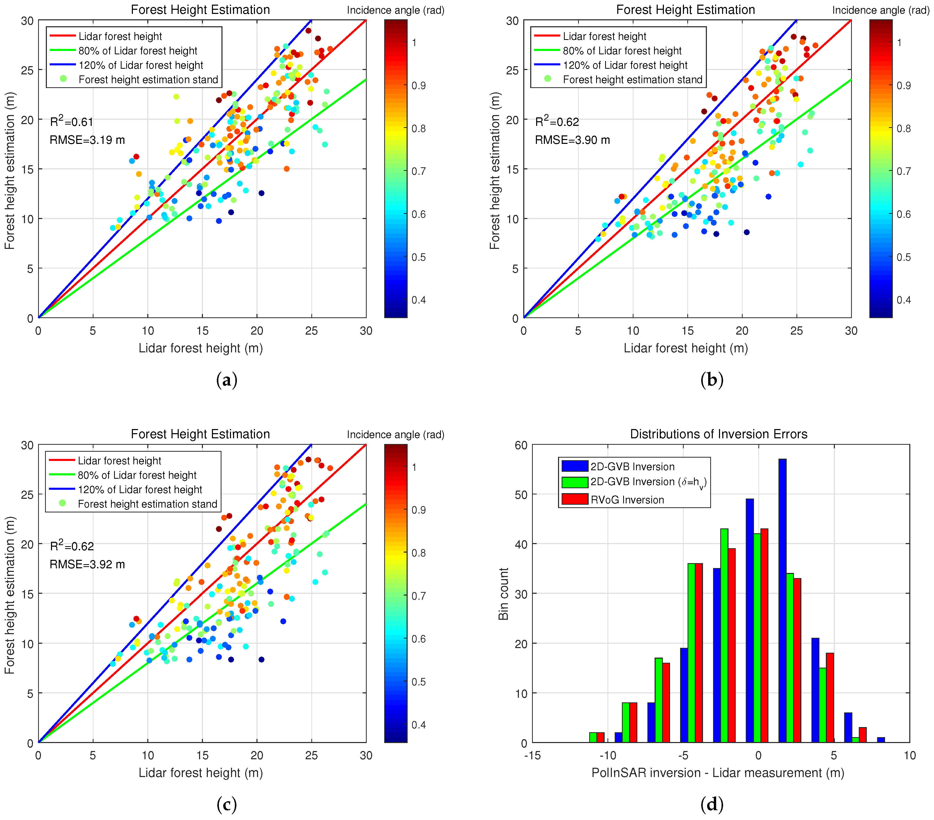
In line with the flowchart in Figure 6, the Pol-InSAR process is first implemented to acquire the multi-polarization coherences. In the process of coherence estimation, the coherence optimization is used to suppress the influence of noise and other interferences [38]. The forest height inversion is completed by inputting the estimated Pol-InSAR coherences into Equation (17), which is an optimization process weighted by multi-baseline observations. In this paper, three P-band Quad-pol interferometric pairs with uniform spatial baseline sampling are applied, as shown in Table 1. 200 verification stands are randomly selected to assess the inversion performance. The pixels in the same stand have similar LiDAR forest heights.

Besides the two-dimensional GVB inversion (consisting of $\delta =h_v$ and $\delta =0$), the two-dimensional GVB with only $\delta =h_v$ inversion and the RVoG inversion are carried out as well. Based on Equations (10) and (17), all these three inversions use a three-baseline configuration to increase observation spaces, thereby avoiding the assumption of null ground-to-volume ratio. In line with the previous analysis, the advantage of two-dimensional GVB model over RVoG model is that the former not only has the solution space corresponding to $\delta =h_v$ (the green curves in Figure 5), but also has the solution space corresponding to $\delta =0$ (the blue curves in Figure 5) which is actually a complement to the RVoG model. Therefore, theoretically, the inversion performance of the two-dimensional GVB model with only $\delta =h_v$ should be very similar to that of the RVoG model, and the performance of these two inversions should be inferior to that of the two-dimensional GVB model containing both $\delta =h_v$ and $\delta =0$.

The inversions corresponding to the two-dimensional GVB model (Figure 8a), the two-dimensional GVB model with only $\delta =h_v$ (Figure 8b) and the RVoG model (Figure 8c) are presented in Figure 8. The root mean square error (RMSE) of the three inversions is 3.19 m, 3.90 m, and 3.92 m in turn. The homologous correlation coefficients $R^2$ are 0.61, 0.62 and 0.62. Consistent with the theoretical analysis, the performance of the two-dimensional GVB with only $\delta =h_v$ inversion and the RVoG inversion are very close. Simultaneously, it can be seen that these two inversions still present a certain degree of underestimation, which cannot be compensated by a multi-baseline configuration. After adding the case $\delta =0$ to the two-dimensional GVB solution space, the underestimation can be alleviated. Compared with the two-dimensional GVB with only $\delta =h_v$ inversion and the RVoG inversion, the two-dimensional GVB inversion improves the performance by 18.21% and 18.62% respectively, which indicates the superiority of the proposed two-dimensional GVB model containing both $\delta =h_v$ and $\delta =0$. Since the three correlation coefficients $R^2$ are very close, this indicator cannot reflect the performance difference of different inversions. In addition, the statistical histogram of the differences between the above three inversions and the LiDAR measurement is shown in Figure 8d, which clearly reflects the underestimation of the two-dimensional GVB with only $\delta =h_v$ inversion and the RVoG inversion, and the improvement of the two-dimensional GVB inversion for this underestimation.

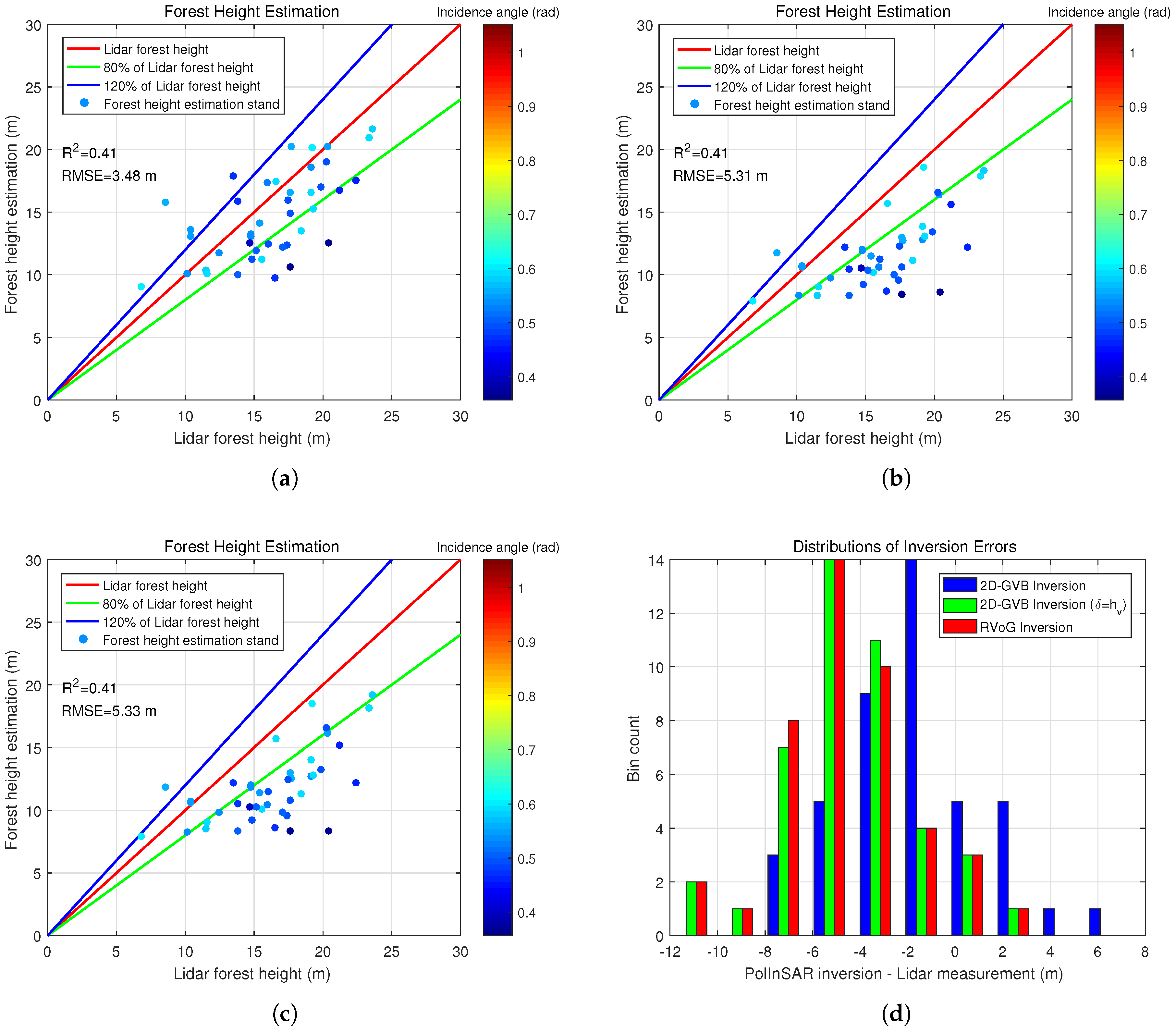
In line with the previous work [17,23,25], the multi-baseline RVoG inversion has a relatively satisfactory performance in the region with a large incidence angle, while the underestimation mainly exists in the region with a small incidence angle. As a result, the following analysis will focus on the inversion performance in the small incidence angle region. The stands with an incidence angle less than 0.6 rad (the lower the threshold is set, the more significant the performance difference) in Figure 8 are selected for quantitative evaluation, as shown in Figure 9. The RMSEs of the three inversions are 3.48 m, 5.31 m and 5.33 m, and the homologous correlation coefficients $R^2$ are 0.41, 0.41 and 0.41. Compared with Figure 8a, the two-dimensional GVB inversion in Figure 9a maintains almost the same RMSE, which indicates that the inversion has a stable performance over the entire incidence angle range. Nevertheless, compared with Figure 8b,c, the two-dimensional GVB with only $\delta =h_v$ inversion (Figure 9b) and the RVoG inversion (Figure 9c) deteriorated in the region with a small incidence angle. Specifically, the performance of these two inversions is reduced by 36.15% and 35.97%, respectively. This is because the two-dimensional GVB model with only $\delta =h_v$ and the RVoG model are more effective in the region with a large incidence angle, while the two-dimensional GVB model with only $\delta =0$ mainly works in the region with a small incidence angle. Therefore, the performance improvement of the proposed two-dimensional GVB inversion is more obvious in the area of small incidence angle, whose accuracy is improved by 34.46% and 34.71% compared to Figure 9b,c, respectively. Similarly, from the histogram in Figure 9d, it is apparent that the two-dimensional GVB inversion has a significant performance improvement over the two-dimensional GVB with only $\delta =h_v$ inversion and the RVoG inversion.

5. Discussions and Conclusions

Since the research in this paper is based on P-band Pol-InSAR observations, the characteristics of P-band SAR systems were consistently the focus of the entire research. This paper analyzes the relationships between model parameters and observation spaces (observation baselines). To ensure that the RVoG optimization has a unique solution, the single-baseline inversion must be combined with certain rules (such as the null ground-to-volume ratio assumption or guessing a model parameter based on prior knowledge in advance) [17]. The multi-baseline inversion becomes an effective choice when the null ground-to-volume ratio assumption is no longer valid (such as the sparse boreal forest under P-band observations) and a parameter in the model cannot be accurately predetermined. Furthermore, under P-band observations, the forest canopy exhibits vertical structure heterogeneity, which makes it necessary to adjust the traditional RVoG model that uses the exponential function to describe the forest vertical structure. This paper approximates $\delta \ge h_v$, $\delta \le 0$ and $\delta \in \left(0, h_v\right)$ in GVB model as $\delta =h_v$, $\delta =0$ and a constant volume profile, thereby simplifying the three-dimensional GVB model into a two-dimensional GVB model. The two-dimensional GVB model achieves dimensionality reduction while retaining the advantage of the GVB model over the RVoG model (that is, increasing the solution space corresponding to $\delta =0$ in the GVB model). Due to the same mathematical conditions as the RVoG model, the two-dimensional GVB model optimization also requires a multi-baseline configuration.

The experimental results illustrate that there is clear dependence of the RVoG inversion accuracy from the incidence angle. A possible reasonable explanation is that the penetration depth of the electromagnetic wave into the canopy is negatively related to the incidence angle. Specifically, the RVoG model presents an underestimation in the region with a small incidence angle, while this underestimation can be improved by the proposed two-dimensional GVB model. The reason for the underestimation improvement is that the vertical backscatter profile is closer to Figure 4c, which cannot be expressed by the RVoG model. The corresponding solution space is represented by the blue curves in Figure 5. When the solution volume only coherence is located in this supplementary solution space (e.g., the blue dot in Figure 5), the inversion performance based on the two-dimensional GVB model will be better than that based on the RVoG model.

Compared with the previous work [25], the proposed method achieves similar accuracy while simplifies the inversion process. Furthermore, the regularity among the parameters used in reference [25] depends on the specific experimental data, which may not be universal. In contrast, the method proposed in this paper has more advantages in general adaptability.

Some limitations are also noteworthy. Compared to the single-baseline, the multi-baseline configuration increases the complexity of the optimization process. In practice, since it may fall into an optimization without physical significance, the multi-baseline inversion depends to some extent on optimization initial values and constraints [24,25]. Therefore, a possible solution is to substitute with the single-baseline configuration to optimize the two-dimensional GVB model to avoid multi-baseline instability. According to the relationships between independent observation equations and unknown parameters based on the single-baseline configuration, the realization of the single-baseline inversion depends on certain prior knowledge, which may be feasible due to a large number of data sources obtained by multi-sensor at present. Furthermore, the reason for simplifying the three-dimensional GVB model is that it is too complicated and causes great difficulties in the inversion process, and yet this simplification may introduce some errors. Although the appearance of the errors may rely on specific experimental data, it is meaningful to carry out an analysis on the errors introduced by the simplification operation, which may become a key aspect of future research.

References

- Treuhaft, R.N.; Madsen, S.N.; Moghaddam, M.; Van Zyl, J.J. Vegetation characteristics and underlying topography from interferometric radar. Radio Sci. 1996, 31, 1449–1485. [Google Scholar] [CrossRef]
- Cloude, S.R.; Papathanassiou, K.P. Polarimetric SAR interferometry. IEEE Trans. Geosci. Remote Sens. 1998, 36, 1551–1565. [Google Scholar] [CrossRef]
- Treuhaft, R.N.; Cloude, S.R. The structure of oriented vegetation from polarimetric interferometry. IEEE Trans. Geosci. Remote Sens. 1999, 37, 2620–2624. [Google Scholar] [CrossRef]
- Treuhaft, R.N.; Siqueira, P.R. Vertical structure of vegetated land surfaces from interferometric and polarimetric radar. Radio Sci. 2000, 35, 141–177. [Google Scholar] [CrossRef] [Green Version]
- Papathanassiou, K.P.; Cloude, S.R. Single-baseline polarimetric SAR interferometry. IEEE Trans. Geosci. Remote Sens. 2001, 39, 2352–2363. [Google Scholar] [CrossRef] [Green Version]
- Cloude, S.R.; Papathanassiou, K.P. Three-stage inversion process for polarimetric SAR interferometry. Proc. Inst. Elect. Eng. Radar Sonar Navig. 2003, 150, 125–134. [Google Scholar] [CrossRef] [Green Version]
- Cloude, S.R. Polarisation: Applications in Remote Sensing; Oxford University Press: Oxford, UK, 2009. [Google Scholar]
- Cloude, S.R. Robust parameter estimation using dual baseline polarimetric SAR interferometry. In Proceedings of the IEEE International Geoscience and Remote Sensing Symposium, Toronto, ON, Canada, 24–28 June 2002; pp. 838–840. [Google Scholar]
- Mette, T.; Kugler, F.; Papathanassiou, K.P.; Hajnsek, I. Forest and the random volume over ground—Nature and effect of 3 possible error types. In Proceedings of the European Conference on Synthetic Aperture Radar, Dresden, Germany, 16–18 May 2006. [Google Scholar]
- Garestier, F.; Dubois-Fernandez, P.C.; Papathanassiou, K.P. Pine forest height inversion using single-pass X-band PolInSAR data. IEEE Trans. Geosci. Remote Sens. 2008, 46, 59–68. [Google Scholar] [CrossRef]
- Neumann, M.; Saatchi, S.S.; Ulander, L.M.H.; Fransson, J.E.S. Assessing performance of L-and P-band polarimetric interferometric SAR data in estimating boreal forest above-ground biomass. IEEE Trans. Geosci. Remote Sens. 2012, 50, 714–726. [Google Scholar] [CrossRef]
- López-Martínez, C.; Alonso-González, A. Assessment and estimation of the RVoG model in polarimetric SAR interferometry. IEEE Trans. Geosci. Remote Sens. 2014, 52, 3091–3106. [Google Scholar] [CrossRef]
- Lei, Y.; Siqueira, P. Estimation of forest height using spaceborne repeat-pass L-band InSAR correlation magnitude over the US state of Maine. Remote Sens. 2014, 6, 10252–10285. [Google Scholar] [CrossRef] [Green Version]
- Ballester-Berman, J.D.; Vicente-Guijalba, F.; Lopez-Sanchez, J.M. A simple RVoG test for PolInSAR data. IEEE J. Sel. Top. Appl. Earth Obs. Remote Sens. 2015, 8, 1028–1040. [Google Scholar] [CrossRef] [Green Version]
- Kugler, F.; Koudogbo, F.N.; Gutjahr, K.; Papathanassiou, K.P. Frequency effects in Pol-InSAR forest height estimation. In Proceedings of the European Conference on Synthetic Aperture Radar, Dresden, Germany, 16–18 May 2006. [Google Scholar]
- Garestier, F.; Dubois-Fernandez, P.C.; Champion, I. Forest height inversion using high-resolution P-band Pol-InSAR data. IEEE Trans. Geosci. Remote Sens. 2008, 46, 3544–3559. [Google Scholar] [CrossRef]
- Kugler, F.; Lee, S.-K.; Papathanassiou, K.P. Estimation of forest vertical structure parameter by means of multi-baseline Pol-InSAR. In Proceedings of the IEEE International Geoscience and Remote Sensing Symposium, Cape Town, South Africa, 12–17 July 2009; pp. IV-721–IV-724. [Google Scholar]
- Garestier, F.; Dubois-Fernandez, P.C.; Guyon, D.; Le Toan, T. Forest biophysical parameter estimation using L- and P-band polarimetric SAR data. IEEE Trans. Geosci. Remote Sens. 2009, 47, 3379–3388. [Google Scholar] [CrossRef]
- Lee, S.-K.; Kugler, F.; Hajnsek, I.; Papathanassiou, K.P. The potential and challenges of polarimetric SAR interferometry techniques for forest parameter estimation at P-band. In Proceedings of the European Conference on Synthetic Aperture Radar, Aachen, Germany, 7–10 June 2010; pp. 503–505. [Google Scholar]
- Dubois-Fernandez, P.C.; Souyris, J.-C.; Angelliaume, S.; Garestier, F. The compact polarimetry alternative for spaceborne SAR at low frequency. IEEE Trans. Geosci. Remote Sens. 2008, 46, 3208–3222. [Google Scholar] [CrossRef]
- Roueff, A.; Arnaubec, A.; Dubois-Fernandez, P.C.; Refregier, P. Cramer-rao lower bound analysis of vegetation height estimation with random volume over ground model and polarimetric SAR interferometry. IEEE Geosci. Remote Sens. Lett. 2011, 8, 1115–1119. [Google Scholar] [CrossRef]
- Arnaubec, A.; Roueff, A.; Dubois-Fernandez, P.C.; Réfrégier, P. Vegetation height estimation precision with compact PolInSAR and homogeneous random volume over ground model. IEEE Trans. Geosci. Remote Sens. 2014, 52, 1879–1891. [Google Scholar] [CrossRef]
- Hajnsek, I.; Scheiber, R.; Keller, M.; Horn, R.; Lee, S.-K.; Ulander, L.; Gustavsson, A.; Sandberg, G.; Le Toan, T.; Tebaldini, S.; et al. BIOSAR 2008: Final Report. 2009. Available online: https://earth.esa.int/c/document_library/get_file?folderId=21020&name=DLFE-903.pdf (accessed on 21 November 2018).
- Fu, H.; Wang, C.; Zhu, J.; Xie, Q.; Zhang, B. Estimation of pine forest height and underlying DEM using multi-baseline P-band PolInSAR data. Remote Sens. 2016, 8, 820. [Google Scholar] [CrossRef] [Green Version]
- Sun, X.; Wang, B.; Xiang, M.; Jiang, S.; Fu, X. Forest height estimation based on constrained Gaussian vertical backscatter model using multi-baseline P-band Pol-InSAR data. Remote Sens. 2019, 11, 42. [Google Scholar] [CrossRef] [Green Version]
- Xie, Q.; Zhu, J.; Wang, C.; Fu, H.; Lopez-Sanchez, J.M.; Ballester-Berman, J.D. A modified dual-baseline PolInSAR method for forest height estimation. Remote Sens. 2017, 9, 819. [Google Scholar] [CrossRef] [Green Version]
- Garestier, F.; Le Toan, T. Forest modeling for height inversion using single-baseline InSAR/Pol-InSAR data. IEEE Trans. Geosci. Remote Sens. 2010, 48, 1528–1539. [Google Scholar] [CrossRef]
- Garestier, F.; Le Toan, T. Estimation of the backscatter vertical profile of a pine forest using single baseline P-band (Pol-)InSAR data. IEEE Trans. Geosci. Remote Sens. 2010, 48, 3340–3348. [Google Scholar] [CrossRef]
- Hajnsek, I.; Kugler, F.; Lee, S.-K.; Papathanassiou, K.P. Tropical-forest-parameter estimation by means of Pol-InSAR: The INDREX-II campaign. IEEE Trans. Geosci. Remote Sens. 2009, 47, 481–493. [Google Scholar] [CrossRef] [Green Version]
- Kugler, F.; Lee, S.-K.; Hajnsek, I.; Papathanassiou, K.P. Forest height estimation by means of Pol-InSAR data inversion: The role of the vertical wavenumber. IEEE Trans. Geosci. Remote Sens. 2015, 53, 5294–5311. [Google Scholar] [CrossRef]
- Bamler, R.; Hartl, P. Synthetic aperture radar interferometry. Inverse Probl. 1998, 14, R1–R54. [Google Scholar] [CrossRef]
- Lavalle, M.; Simard, M.; Hensley, S. A temporal decorrelation model for polarimetric radar interferometers. IEEE Trans. Geosci. Remote Sens. 2012, 50, 2880–2888. [Google Scholar] [CrossRef]
- Lavalle, M.; Khun, K. Three-baseline InSAR estimation of forest height. IEEE Geosci. Remote Sens. Lett. 2014, 11, 1737–1741. [Google Scholar] [CrossRef]
- Park, S.-E.; Moon, W.M.; Pottier, E. Assessment of scattering mechanism of polarimetric SAR signal from mountainous forest areas. IEEE Trans. Geosci. Remote Sens. 2012, 50, 4711–4719. [Google Scholar] [CrossRef]
- Lu, H.; Suo, Z.; Guo, R.; Bao, Z. S-RVoG model for forest parameters inversion over underlying topography. Electron. Lett. 2013, 49, 618–620. [Google Scholar] [CrossRef]
- Zhang, Q.; Liu, T.; Ding, Z.; Zeng, T.; Long, T. A modified three-stage inversion algorithm based on R-RVoG model for Pol-InSAR data. Remote Sens. 2016, 8, 861. [Google Scholar] [CrossRef] [Green Version]
- Sun, X.; Wang, B.; Xiang, M.; Fu, X.; Zhou, L.; Li, Y. S-RVoG model inversion based on time-frequency optimization for P-band polarimetric SAR interferometry. Remote Sens. 2019, 11, 1033. [Google Scholar] [CrossRef] [Green Version]
- Tabb, M.; Orrey, J.; Flymn, T.; Carande, R. Phase diversity: A decomposition for vegetation parameter estimation using polarimetric SAR interferometry. In Proceedings of the European Conference on Synthetic Aperture Radar, Cologne, Germany, 4–6 June 2002; pp. 721–724. [Google Scholar]
Figure 1.
The profile of Random Volume over Ground model.
Figure 2.
The profile of Gaussian vertical backscatter volume over ground. (a): ; (b): ; (c): .
Figure 3.
The solution space of Gaussian vertical backscatter model when or is fixed. Each blue or red curve represents the volume only coherence for a given forest height at an interval of 1 m. The terrain slope is set to 0.
Figure 4.
The profile of two-dimensional Gaussian vertical backscatter volume over ground. (a): ; (b): constant volume profile; (c): .
Figure 5.
The solution space of two-dimensional Gaussian vertical backscatter model. Each blue or green curve, or red dot represents the volume only coherence for a given forest height at an interval of 1 m. The terrain slope is set to 0. The blue dot refers to the solution volume only coherence, and the minimum distance between it and the solution space is indicated by the black dotted line. is the final solution in solution space, while corresponds to the solution forest height in solution space. Both and lie on the solution space curve of the constant profile.
Figure 6.
Flowchart of the proposed two-dimensional GVB modeling and multi-baseline inversion.
Figure 7.
Pauli-basis polarization composite map.
Figure 8.
The forest height estimation of validation stands with (a) two-dimensional GVB model, (b) two-dimensional GVB model with only , and (c) RVoG model, compared with the LiDAR measurement. The histogram (d) shows the differences between the Pol-InSAR inversion and the LiDAR measurement with the two-dimensional GVB model, two-dimensional GVB model with only , and RVoG model, respectively. The stands that are counted in (d) correspond to the stands in (a–c).
Figure 9.
The forest height estimation of validation stands with (a) two-dimensional GVB model, (b) two-dimensional GVB model with only , and (c) RVoG model, compared with the LiDAR measurement. These validation stands correspond to those in Figure 8 with an incidence angle less than 0.6 rad. The histogram (d) shows the differences between the Pol-InSAR inversion and the LiDAR measurement with the two-dimensional GVB model, two-dimensional GVB model with only , and RVoG model, respectively. The stands that are counted in (d) correspond to the stands in (a–c).