Performance Analysis of Open Source Time Series InSAR Methods for Deformation Monitoring over a Broader Mining Region

Laboratory of Remote Sensing, National Technical University of Athens, 9 Heroon Polytechniou Str., Zographos, 15790 Athens, Greece
*
Author to whom correspondence should be addressed.
Remote Sens. 2020, 12(9), 1380; https://0-doi-org.brum.beds.ac.uk/10.3390/rs12091380
Submission received: 30 March 2020
/
Revised: 21 April 2020
/
Accepted: 24 April 2020
/
Published: 27 April 2020
(This article belongs to the Special Issue Scaling-Up Deformation Monitoring and Analysis)
Abstract
:Time Series Interferometric Synthetic Aperture Radar (TSInSAR) methods have been widely and successfully applied for spatiotemporal ground deformation monitoring. The main groups of methodological approaches are often referred to as Persistent Scatterer (PS), Small Baseline (SB), and hybrid approaches that incorporate PS and SB concepts. While TSInSAR techniques have long been able to provide accurate deformation rates for various applications, their corresponding performance in complex environments such as mining areas has to be investigated. This study focuses on comparing the performance of three open source TSInSAR toolboxes (Stamps, Giant, Mintpy) over an extended region that includes an active opencast coal mine. We present the deformation results of each TSInSAR method on a Sentinel-1 dataset of 125 acquisitions spanning around 2.5 years over the Ptolemaida-Florina coal mine site that is characterized by several environmental and surface deformation conditions. First, a cross-comparison analysis is presented over different land cover classes. The study shows that all TSInSAR methods are capable for generating similar ground deformation results when the area has stable ground scattering conditions and the dataset sufficient temporal sampling. The most controversial results between TSInSAR approaches were found in land cover classes that include medium to high vegetation. An external comparative analysis between the different results from TSInSAR methods and leveling measurements is also performed. Stamps approach presented the best agreement with the in-situ deformation rates. The Giant approach yielded the best cumulative deformation results due to our a priori knowledge of temporal behavior of deformation in the vicinity of the leveling locations. Finally, we discuss the main pros and cons of each TSInSAR approach and we highlight the importance of comparison analysis that can provide insights and can lead to better interpretation of the results.
1. Introduction and Motivation
Ground movements and surface deformation on mines can lead to instabilities and slope failures that can cause risks to personnel, equipment, and production [1]. The main limitations in our ability to monitor deformation in mining regions are the difficult and fast changing conditions caused by the ongoing mining activity. In order to successfully monitor the complex spatial and temporal behavior of the deformation in mining regions, a monitoring system with suitable spatial density of measurement points (MPs) with a high measurement frequency is required. In most cases, the monitoring techniques of such a system can be divided into two main categories. The first category is related to surveying techniques that determine the absolute and relative positions of certain points. The most popular surveying instruments that are commonly used are GNSS (Global Navigation Satellite Systems), total stations, levels, Terrestrial Laser scanners, Ground-based SARs, and photogrammetric cameras. The second category is related to the use of geotechnical equipment such as extensometers, piezometers, inclinometers, etc. The aforementioned conventional techniques can provide high quality measurements but are limited by their operation and maintenance cost.
Due to the high maintenance and operation cost of the aforementioned deformation monitoring strategies, alternative approaches based on remote sensing data can potentially improve the monitoring procedure in terms of cost and accuracy. TSInSAR methodologies are capable of extracting the time series of ground deformation from a set of SAR acquisitions [2]. The accuracy and precision of the extracted ground deformation can vary due to decorrelation of the SAR signal. The main decorrelation factors of the SAR signal are the atmospheric delay, phase unwrapping errors, and changes of the backscattering mechanism of the targets over time [3]. The most popular TSInSAR approaches that tackle the aforementioned limitations are described in the following paragraphs.
The oldest and first group of TSInSAR approaches focuses on a subset of points (called measurement points) that have high phase stability and are referenced as persistent scatterer (PS) methods [4,5,6,7]. PS methodologies extract the measurement points from a single-master network interferograms and can achieve even submillimeter accuracy [8]. The main selection strategies of the measurement points are based on their phase variation in time [4] or on the correlation of their phase variation in space [7]. Many applications of PS methods can be found for urban environments. An open-source implementation of a PS methodology is provided by Stamps toolbox [7,9].
The second group of TSInSAR approaches focuses on exploiting a redundant network of multi-master interferograms that have small temporal and spatial baselines. These approaches are referred to as small baseline subset (SBAS) methods [10]. The network of the SBAS methods consists of unwrapped interferograms that can be fully-connected or form isolated clusters over time. Fully-connected networks are inverted using least square estimation or L1-norm minimizations [11]. Non-fully connected networks are inverted/solved using singular value decomposition or a regularization constraint to obtain physically sound solutions [10,12]. Open sources implementations of SBAS methodologies are provided in several software packages, such as GMTSAR [13], Giant [14], Stamps [9], MSBAS [15], Pyrate [16], and Mintpy [17].
The third group of TSInSAR approaches exploits all the possible interferograms of a given set of SLC acquisitions [18,19,20]. Similar to the aforementioned techniques, the goal of the network inversion is to obtain optimal and noise-limited phases of the given SAR acquisitions. Maximum likelihood estimator [21] and eigenvalue decomposition of the covariance matrix [22,23] are some of the tools that can be used for optimal phase estimation. The main characteristic of these methods is that the network inversion is performed before phase unwrapping. Another important characteristic of these methods is the preprocessing of the distributed scatterers in order to be processed by PS algorithms. The preprocessing step enables the joint processing of distributed and persistent scatterers, which increases coverage with high accuracy deformation retrieval. This is due to the fact that the estimator of distributed scatterer signal provides a triangular phase that enables spatiotemporal (3D) unwrapping, which is superior to 2D unwrapping [24]. The main limitation of these techniques is the computational complexity given the big volume of SAR data. Currently, to our knowledge, no open-source implementations are available.
Despite the maturity of TSInSAR approaches, the unprecedented big volume of SAR data has not been fully exploited. Sentinel-1 constellation provides a big streamline of SAR data that can potentially be used for ground deformation monitoring solutions. Therefore, we believe there is room for experimentation related to potential capabilities over mining regions. In the mining world, to our knowledge, there are only a few organizations that are using TSInSAR deformation results in existing deformation monitoring systems. Open source tools play a crucial role with respect to this. Nowadays, the availability of the TSInSAR algorithms will enable mining organizations and interested stakeholders to generate on their own SAR derived ground deformation estimations. Given the fact that most of the mining organizations perform ground surveys for deformation measurements, open source TSInSAR estimations can be assessed and validated, and capabilities and limitations of each TSInSAR approach can be pointed out. However, an assessment and comparison approach of the results between different TSInSAR approaches and the in-situ measurements is missing. In fact, this will not only provide best practices and insights on the preferred existing methodological strategies over mining regions but also will potentially support the rapid evolution of algorithmic approaches that will make optimal use of big data in terms of accuracy and computational cost.
This study helps to bridge the gap between the InSAR and mining world by providing an automated workflow that performs the comparison of results of several open source algorithmic approaches that are described in Section 2, namely: Stamps [9], Giant [14], and Mintpy [17]. The processing steps that perform the comparison of interferometric time series methodologies are described in detail. The main objectives and research questions that this study attempts to answer are:
- Compare the performance of open source algorithmic approaches over a complex opencast mining environment.
- Present the positive and negative sides of each algorithmic approach with respect to environmental conditions, accuracy, and spatial coverage.
- Present the critical factors that are related with the performance of each algorithmic strategy and present some best practices.
- Provide a standardized methodology for comparing the results provided by the employed TSInSAR tools.
In Section 2, the theoretical concept of each open source algorithmic implementation used in this study is discussed. In Section 3, the area of the case study, an extended region focused on Ptolemaida-Florina coal mine in Greece, and the datasets used are described. The results of each TSInSAR approach and a comparison analysis between the TSInSAR deformation results with the in-situ measurements, are presented in Section 4. Based on the theoretical concepts of each algorithm and the respective results, a comprehensive discussion is presented in Section 5. In Section 6, the conclusions of this study are outlined and suggestions for conducting future TSInSAR deformation studies over (opencast) mining regions are presented.
2. Methods
2.1. Mintpy-Miami InSAR Time-Series Software in Python
The Mintpy toolbox is a Python 3 software for small baseline InSAR time series analysis. The input is a stack of differential interferograms that form a fully connected network. Interferograms have to be already unwrapped with small geometric perpendicular and temporal baselines for maximizing their quality. For modern SAR constellations with small orbital tube and short revisit time, such as Sentinel-1, a fully connected network of interferograms can easily be formed. The input stack can be generated using, among other tools, the Interferometric SAR Scientific Computing Environment ISCE [25]. The main steps of the interferometric processing performed by ISCE are orbit correction, de-burst, co-registration, interferogram generation and adaptive filtering, subtraction of topographic phase using given Digital Elevation Model (DEM), and 2D (space) unwrapping.
The Mintpy toolbox consists of three main processing steps: (a) the raw interferometric phase time series calculation; (b) the correction of the raw phase time series from error sources; and (c) the noise evaluation step that results in the exclusion of noise SAR acquisitions and the final calculation of noise-reduced displacement time series. Moreover, in order to have a quality index for the extracted deformation values, temporal coherence is calculated for each pixel according to [26].
The first processing step of Mintpy is the inversion of the input redundant, fully connected stack via an unbiased weighted least square estimator in order to acquire raw time series of interferometric phase for each date. The weight information can be related to a uniform behavior or no weighting [10], spatial coherence at pixel level [27,28], inverse of the phase variance [29], and nonparametric Fisher information matrix (FIM) [23,30]. For this study, only the inverse of the phase variance weighting was selected because, according to [21] and for a small number of looks [17], the inverse of phase variance as a weighting factor gives the most robust and one of the best performances for network inversion.
The second processing step is the correction of the raw inverted phase time-series from phase error sources at the time domain. Deterministic components such as tropospheric delays, topographic residuals, and/or phase ramps are preserved after inversion and can be suppressed in the time-series domain in order to obtain a time series of noise-reduced displacement. Moreover, a correction scheme of 2D unwrapping procedure errors with a variety of approaches is offered. The unwrapping correction method that was selected is related to the phase closure of triplets of interferograms, based on the assumption that the SAR phase field is conservative [31].
The third processing step is the noise evaluation of each SAR acquisition in terms of residual phase. Mintpy considers the residual phase as a combination of residual tropospheric turbulence, uncorrected ionospheric turbulence, and the remaining decorrelation noise. The root mean square error of the residual phase is calculated for each SAR acquisition after a quadratic deramping [32] over the reliable pixels that are used in the network inversion. The identified noisy acquisitions are excluded and the topographic residual and velocity estimation is performed for a second time.
2.2. Giant-Generic InSAR Analysis Toolbox
The Giant toolbox [14] was developed for small baseline InSAR time series analysis in Python 2. It requires a stack of differential geocoded or slant-range unwrapped interferograms for the extraction of ground deformation time evolution information. The input interferogram stack can be generated among other tools using ISCE [25].
The first step is the preparation of the interferograms stack by applying phase correction schemes. Firstly, a deramping correction scheme at a network level [31,33] is applied. Secondly, a tropospheric correction scheme based on ERA-5 atmospheric model [34] is applied.
The next step is the inversion of the interferograms stack to obtain deformation information. Conventional SBAS [10], NSBAS [12,33,35], and Multiscale InSAR Time-Series MInTS [36] are the available inversion choices. Conventional SBAS uses singular value decomposition to redundant information from the interferometric stack to provide ground deformation time series. The main difference of N-SBAS with respect to the conventional SBAS technique is that N-SBAS includes constraints from user predefined temporal functions to join islands of disconnected interferograms. The main differences of MInTS with respect to conventional SBAS technique are firstly the transformation of the interferometric phase into the wavelet domain before the temporal inversion and secondly the description of the time evolution of the ground deformation by predefined functions. In all the strategies, the inversion operation is performed in each pixel separately subject to coherence and valid number of observation criteria. For this study, only Giant-NSBAS approach was employed. The main reason for that is that conventional SBAS and MInTS methods require pixels to be coherent in most/all of the interferometric network, something that is often violated in mining regions.
2.3. Stamps—Stanford Method for Persistent Scatterers
Stamps consists of a PS and a combined PS and SBAS (Stamps/MTI) processing workflow which are briefly described below. Comprehensive algorithm descriptions can be found in [6,9,37].
The Stamps-PS approach is based on spatial correlation of interferometric phases. Conventional PS methodologies [4] extract deformation over high amplitude pixels assuming a well-defined phase history. Furthermore, the phase history of each pixel is compared with a predefined temporal deformation model. Stamps implementation is based on the stable spatial phase characteristics and is able to extract deformation over low-amplitude pixels without prior knowledge of temporal deformation behavior. However, the assumption that the deformation is spatially correlated is not true for isolated movement of individual scatterers which are considered as noise. The Stamps-PS approach has a lot of applications in urban and non-urban areas like volcanic regions.
The combined Stamps/MTI approach is able to combine information from PS and SBAS at a full resolution and has some clear advantages over conventional multilooking SBAS approaches. It was observed that a multilooking procedure may include pixels that completely decorrelate and add noise to the multilooked pixel. In this direction, adaptive multilooking approaches have been developed [19]. The full resolution processing that Stamps/MTI adopts mitigates the noise from traditional boxcar multilooking procedures. Moveover, Stamps/MTI performs the unwrapping of the phase in three dimensions (space and time) and therefore produces more robust results with respect to two-dimensional (space) unwrapping algorithms [7].
Both approaches include a selection strategy of pixels that the deformation information will be extracted. First, for computation reduction reasons, an initial selection of pixels that are expected to be either persistent scatterers or slowly-decorrelating filtered phase (SDFP) pixels through amplitude dispersion analysis [37] is performed. For the selected pixels, a spatially-correlated part of interferometric phase is estimated by bandpass filtering of the surrounding pixels. The spatially-correlated part consists of phase due to ground displacement, atmospheric phase delay, orbit errors, and spatially-correlated height error. Moreover, a spatially-uncorrelated height/DEM error is estimated from its correlation with a perpendicular baseline for each measurement point. By subtracting the spatially-correlated part and the spatially-uncorrelated height error from a raw wrapped interferometric phase, a temporal coherence metric is calculated for each measurement point. Then, a thresholding approach on the aforementioned coherence metric is performed to select the measurement points that are going to be processed.
For this study, the input SLC stack is prepared using ISCE and the Stamps/MTI approach is selected due to its capability to combine information from elements with different scattering characteristics.
2.4. Comparison Methodology
The proposed methodology consists of three steps. The first step is the conversion of the TSInSAR results to vector GIS compatible format with common attributes. Raster datasets from each of the selected open source TSInSAR tools (Stamps, Giant, Mintpy) are converted to TSInSAR point vector datasets mainly for visualization reasons and also to benefit from GIS processing tools. The common structure of the vector data from different TSInSAR tools is suitable for post-processing and comparison analysis.
The second step is the identification of the homologous points between the different TSInSAR point vector datasets. For every pair of vector datasets, a set of points for comparison is selected using a geographical distance criterion. For every point in the first TSInSAR result, the point from the second TSInSAR result with the nearest distance is selected. If this distance is below the predefined geographical distance, then this pair of points will be compared. For each pair of TSInSAR point vector datasets, a vector file including the comparison points is created.
The third step is the calculation of the similarity metrics for each point. Similarity metrics are important for an insightful comparison of time series data. The selection of the similarity metrics is required for optimizing grouping that can potentially reveal distinctive time-dependent processes related with deformation or noise sources. The Euclidean distance metric was selected because it (a) can provide robust results in a wide range of applications [38] and (b) can provide insights because the unit has the same units as the input data. Moreover, the dynamic time warping method [39] has been used. A dynamic time warping method can handle time series that don’t share the same exact time of observations, like the deformation time series that have different observation dates when they come from different sensors, different orbit geometries or result from different algorithms that exclude some observation dates. The Euclidean distance metric is expressed as the Root Mean Square Error (RMSE) by setting the one TSInSAR point vector dataset as reference dataset and the other on as a test dataset. RMSE is calculated according to the following formula:
where is the total number of common used SAR acquisitions for methods A and B, is the homologous point, and is the LOS deformation estimation of method A.
The above steps enable the spatial identification of agreements and disagreements between TSInSAR results in terms of deformation and deformation rates. The spatial identification of these agreements can provide insights regarding the performance of each algorithm. The interested user can focus on particular regions to identify the common deformation patterns or to search potential uncorrected error sources among the different TSInSAR results.
3. Case Study: Ptolemaida-Florina Coal Mine
3.1. Study Area
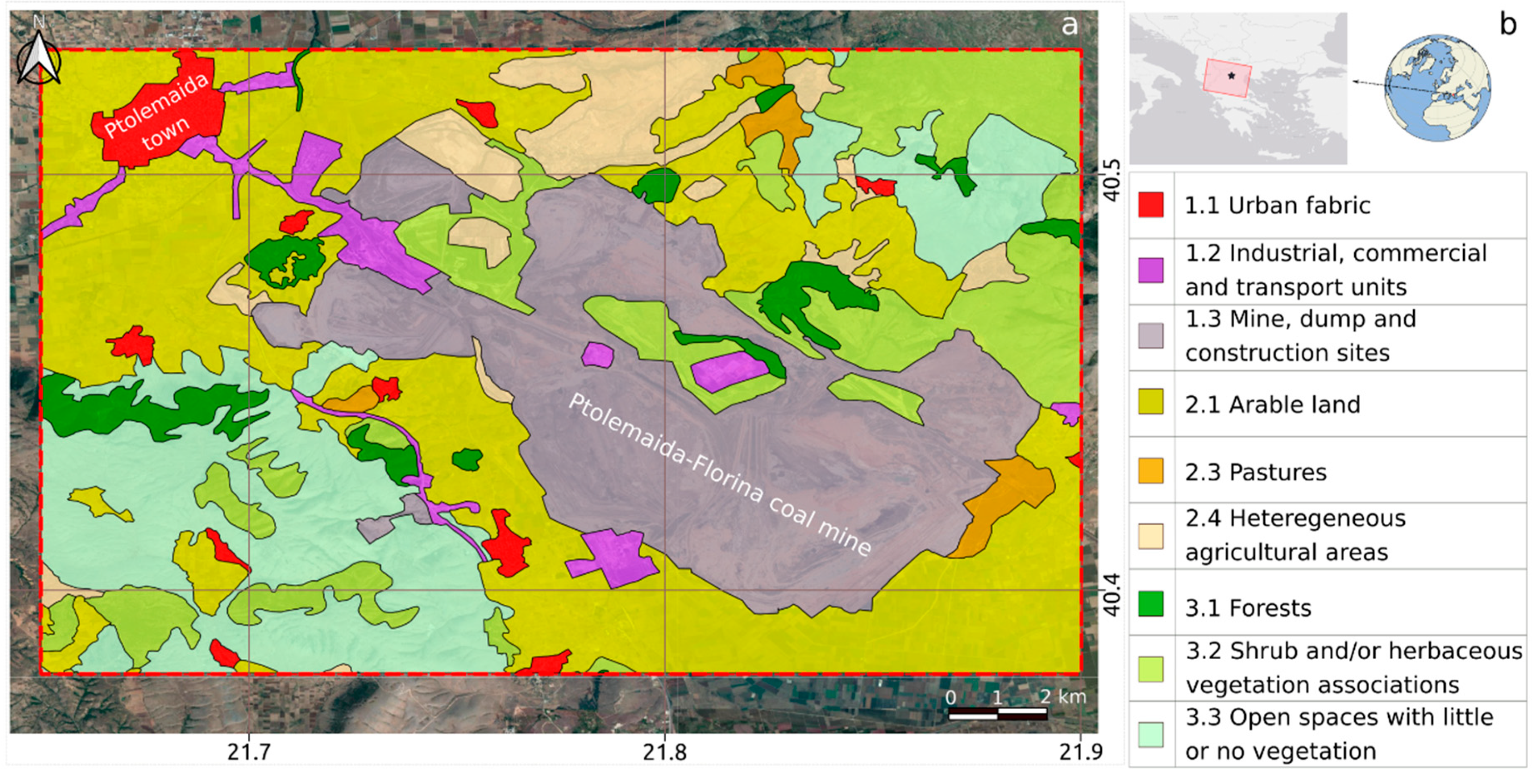
The area of interest is located in the region of Western Macedonia, in Greece, which is one of the most important industrial areas of the country. The land cover classes in the area can be categorized into three main classes according to Corine level-1 land cover classes [40]: artificial surfaces, agricultural areas and forest/semi-natural areas. Interferometric coherence is different for each land cover class and is exploited in a lot of land cover classification studies [41,42]. The different backscattering properties of each land cover can affect the density of the TSInSAR measurements [43] as well as their expected accuracies.
Active mining regions due to fast changing conditions need special treatment. There are regions inside the mine that are under work for certain time periods and other regions that are inactive. Fast changing surface properties result in temporal decorrelation. The study area is included in the dashed red rectangle and is around 357 km2. This work focuses on the part of the Ptolemaida-Florina opencast coal mine, which covers around 90 km2, illustrated with gray color in Figure 1a. Since the 1960s, the Ptolemaida-Florina mine has been one of the main sources of energy production for the country and is owned by Public Power Corporation S.A.-Hellas [44]. The end of 2019, according to the European Commission, the particular coal region will be included in the transition initiative that will lead to mine closure. The gradual decrease of mining operations is an interesting subject for the study of post-mining deformation using TSInSAR techniques.
3.2. Datasets
3.2.1. SAR Data
Due to the expected temporal decorrelation of the mining regions, SAR data from short revisiting (6-day) Sentinel-1 constellation from ESA (European Space Agency) are used. Sentinel-1 consists of two satellites, namely, Sentinel-1A and Sentinel-1B, that were launched in 2014 and 2016, respectively. Sentinel-1 constellation is a polar-orbiting radar imaging system working at C-band (~5.7 cm wavelength). A total of 125 Sentinel-1 TOPS IW acquisitions from the descending track with relative orbit number 80 (Figure 1b), dating from 2016 until the middle of 2018 have been processed. All the data are in the Single Look Complex (SLC) format and only the VV polarization is considered. All the employed S1 acquisitions were snow-free.
3.2.2. In-Situ Deformation Measurements
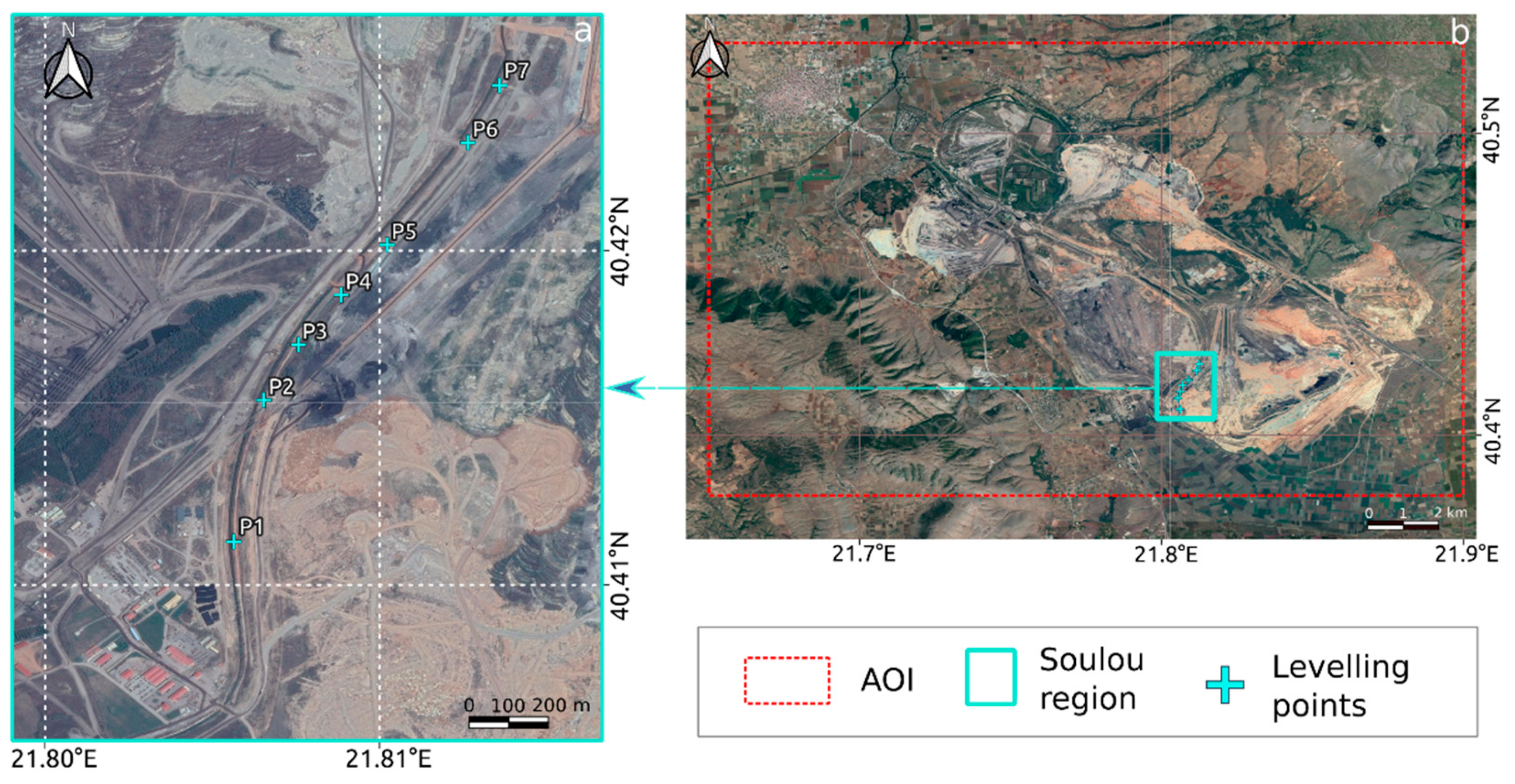
Due to the great importance of the stability of the transportation network, leveling measurements were performed in the “Soulou” region from June 2016 to the end of 2016. Leveling measurements for seven points that are located inside the “Soulou” region (Figure 2) are used for the validation of the TSInSAR results.
3.2.3. Ancillary Data
As an external DEM, we used a photogrammetric DEM with ground pixel size of 5 m, provided by KTIMATOLOGIO S.A. The aforementioned DEM was created in the years 2008–2009 and is more recent with respect to the SRTM DEM.
4. Results and Comparison
4.1. Results
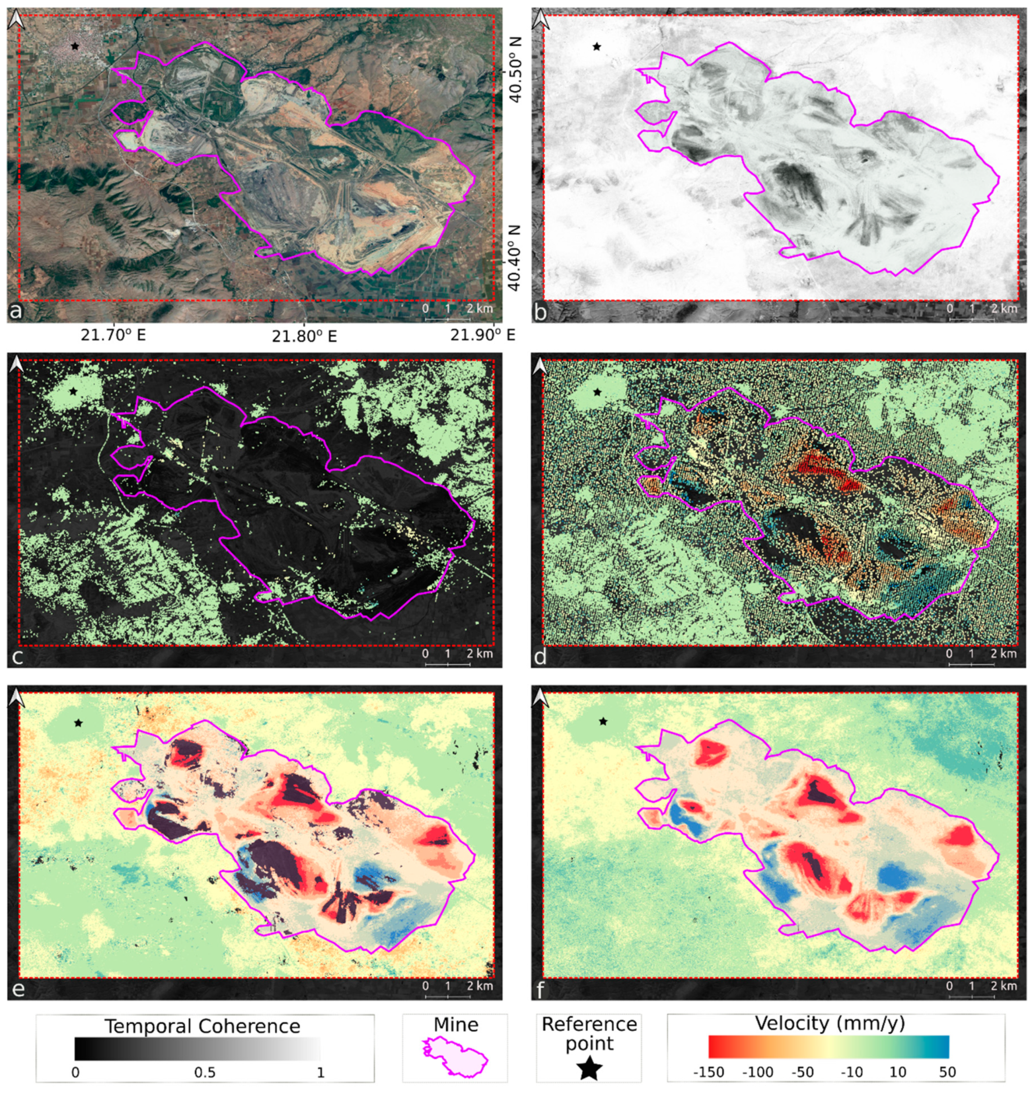
In this section, the generated results of the selected algorithms from the open source TSInSAR software packages are presented (Figure 3). It is important to state that, because of the high inconsistencies in the connected components of the 2D unwrapping procedure resulting from the available 12-day interferograms at the start of 2016, the Mintpy processing was performed only for 6-day interferograms (from October of 2016 until June of 2018). Stamps and Giant results refer to the time span from January 2016 until June 2018. All the results are differential in space and time. They are spatially related to the same reference point (Figure 3) that is located in a very high coherent region of Ptolemaida town. Temporally, the latest date of the SAR acquisition dataset is selected for all the approaches. The temporal reference has been changed to the first available satellite acquisition after the inversion of each algorithm approach. All the results are referring to the Line of Sight (LOS) sensor to target direction.
In Figure 3, it is obvious that the density of measurement points for each selected algorithm is varying. The following can be related with the temporal coherence (Figure 3b) that can be considered as an index for the resulting point density. Temporal coherence can yield values from zero to one. According to Figure 3, over bright regions such as urban areas, rocks, roads, abandoned parts of mining regions, which preserve their scattering properties, a high density and good quality result is expected. Over the darker regions, such as forests, crops, and active mining regions, due to temporal decorrelation, a sparse and low quality result is expected. In particular, Stamps-PS method yielded around 100K measurements points over the high coherence regions. Using the combined Stamps approach that merges PS and SBAS results the measurement points increased to 135K. We point out that oversampling is not implemented in the Stamps processing chain, something that is expected to increase the density of MPs [45]. Mintpy-WSBAS and the NSBAS approach that is included in Giant toolbox outperformed in terms of measurement point density and yielded 900K and 1300K points, respectively. Spatial patterns of ground deformation can be extracted easier from the results of these TSInSAR approaches.
All the algorithms performed similarly over urban areas. The deformation rate of spatial patterns inside the mining area are in agreement for Stamps/MTI, Mintpy-WSBAS, and Giant-NSBAS approaches. Discrepancies between TSInSAR results can be found over low-medium coherent vegetated regions. Even though the Mintpy-WSBAS and Giant-NSBAS approaches yielded denser results, their quality is questionable in vegetated regions. The deformation picture of the vegetated regions is similar for Stamps-PS and Stamps/MTI results only. Thus, further investigation is required to identify and mitigate effects from potential noise sources such as the soil and/or vegetation moisture in forest, mountainous, and crop field regions.
4.2. Cross-Comparison of TSInSAR Results
An RMSE metric is calculated for each pairwise combination of the results provided by the methods (Figure 4). For each pairwise combination, the results of one method are selected as reference dataset and the results of the second method as a test dataset. The RMSE metric is calculated for all the homologous points that are present in both results. Homologous points are selected based on the second step of the comparison methodology [2.4] using a 10 m geographical distance criterion.
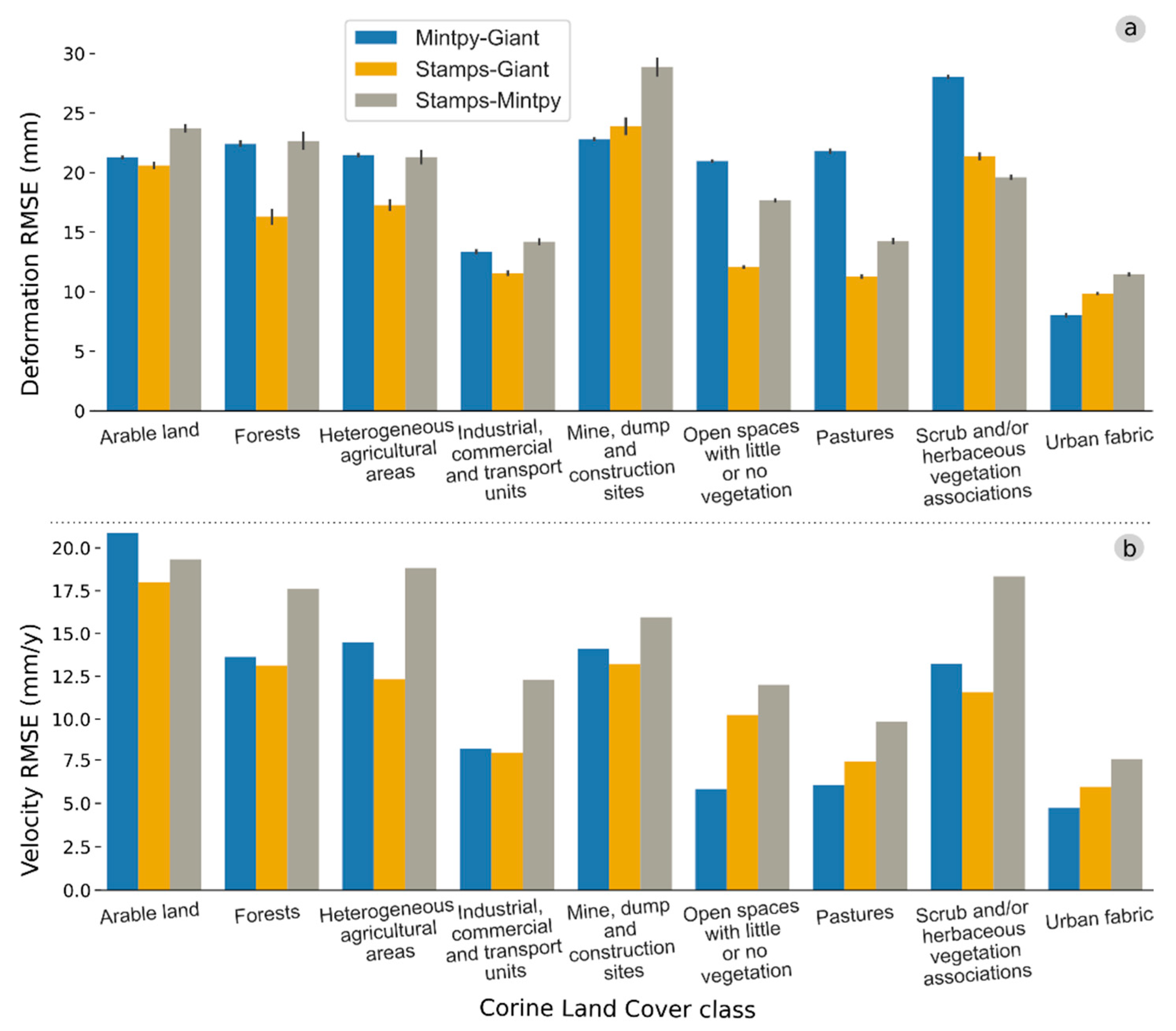
The deformation and deformation rate RMSE values for each Corine land cover level-2 class are presented in Figure 4. In general, the lowest RMSE values were found in industrial, commercial, and transportation units, in open spaces with little or no vegetation, in pastures, and in urban fabric classes. This is expected due to their high coherence with respect to that of other land cover classes (Figure 3b). In land cover classes that include medium to high vegetation, the TSInSAR approaches showed the most controversial results. The different performance of the TSInSAR approaches in the vegetated areas can be related to effects caused by seasonal variation in vegetation density, as well as effects from variations in soil and vegetation moisture. Overall, among the three pairwise combinations (Figure 4), Stamps and Giant results showed the best agreement with each other. The Stamps-Mintpy combination yielded the highest disagreements.
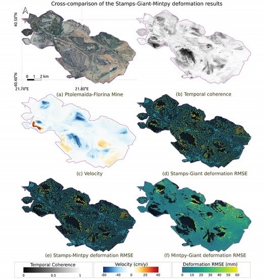
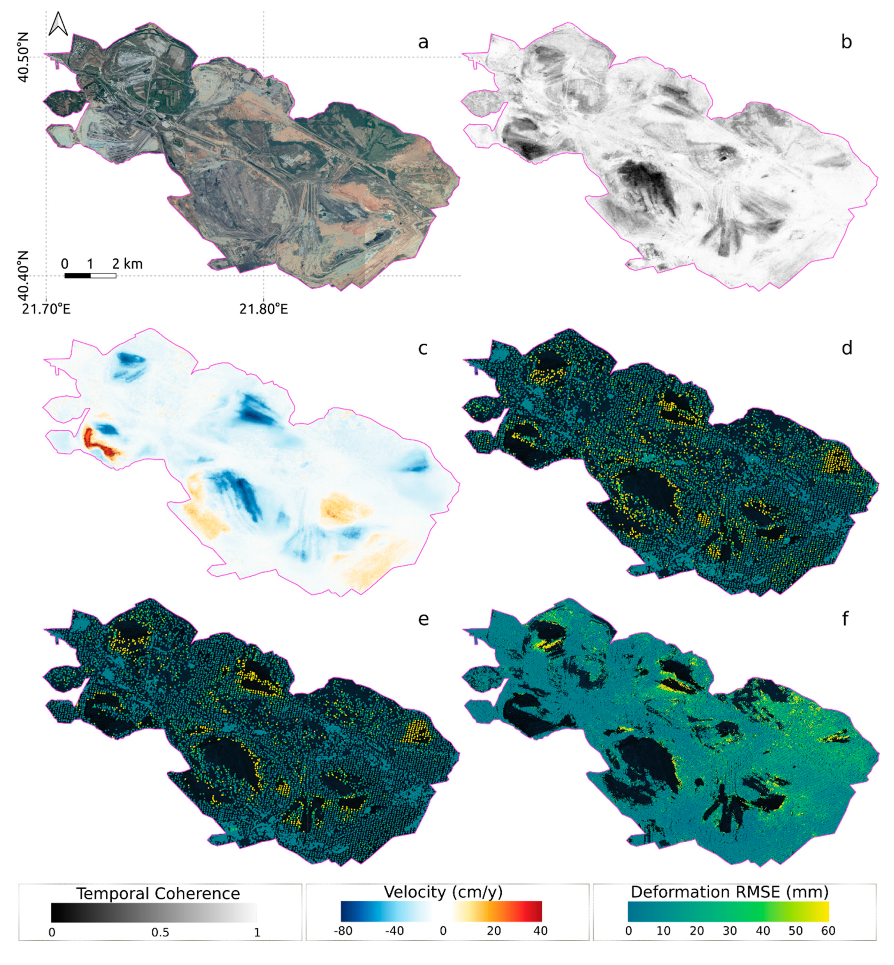
In Figure 5, deformation RMSE maps for all available pairs between the used TSInSAR approaches for the corresponding comparison points [2.4] are presented. TSInSAR approaches were not able to yield results in the high deformation mine regions, which present low temporal coherence (Figure 5b). These regions are observed with very high average deformation velocity in the result provided by Mintpy toolbox [17] (Figure 5c). In the borders of the high deformation regions, big deformation RMSE values, denoted with yellow color (Figure 5d–f), are observed. This occurs because of the low accuracy of the results due to high temporal decorrelation. However, in the stable regions of the mine which are the brightest regions in Figure 5b, TSInSAR approaches yield comparable results, with low RMSEs. These regions are shown with purple color. The regions in the mine for which useful deformation results can be extracted are mainly high coherent regions such as abandoned mining regions, infrastructure, and transportation network.
4.3. External Comparison with In-Situ Leveling Measurement
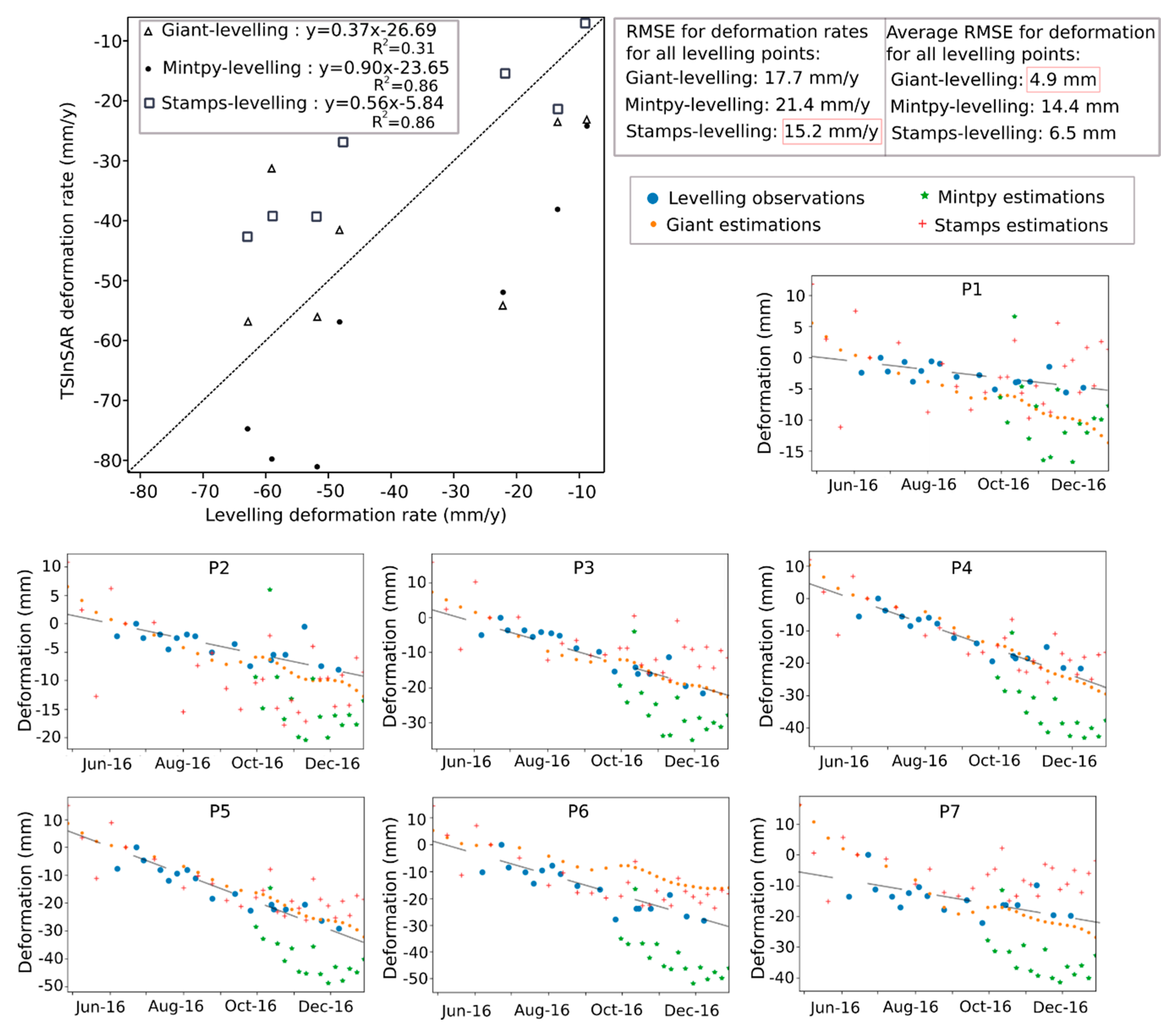
In this section, the comparison of TSInSAR results with leveling measurements is presented. As we already stated, the Mintpy processing was performed only from September of 2016 until June of 2018. The Giant-NSBAS deformation results present a smoothed behavior of the subsidence (Figure 6) due to the inclusion of temporal functions (quadratic in this case) in the design matrix of the system. Mintpy and Stamps results were generated without the use of predefined temporal constraints.
Overall, all of the TSInSAR methods overestimated the subsidence rate according to the regression equations at top left side of Figure 6. Stamps and Mintpy regression equations for deformation rates presented the highest coefficients of determination (0.86). Stamps approach was able to better capture the deformation rate information of the leveling points with an overall RMSE of 15.2 mm/year. Regarding the deformation information, the Giant-NSBAS approach was able to better estimate the leveling observation with an overall RMSE of 5.9 mm. We state that the RMSE values are calculated for the displacements in the LOS direction. In particular, leveling values are projected in the LOS direction by multiplying with the cosine of incidence angle of Sentinel-1 radiation, neglecting horizontal deformation, for the simplicity of validation.
The above results demonstrate that the subsidence behavior on the leveling points can be identified from all the selected open-source methodologies. The regional subsidence is possibly connected with mining operation. However, the interpretation of the deformation patterns is a complex task that requires geological, hydrogeological, and geotechnical information. In order to draw safe conclusions, we believe that the mining schedule activity is also required. For the abovementioned reasons, the interpretation of the subsidence mechanism is omitted at the current stage of this study.
5. Discussion
In this session, the main advantages and limitations of each algorithm are discussed. Then, potential improvements for better monitoring of deformation in mining regions based on our case study results and other recent existing studies are proposed.
The performance of each TSInSAR approach is controlled by the following important factors (Table 1). The first factor is related with the unwrapping procedure of the interferometric phase. Mintpy and Giant software toolboxes require a stack of the differential unwrapped interferograms. In most cases, the unwrapping procedure is performed in space (2D) and for each interferograms separately. 2D unwrapping can produce errors that a sophisticated TSInSAR approach should be able to correct or mitigate their effects. Mintpy includes unwrapping error correction modules [2.1] that can be employed and minimize the impact of the unwrapping errors in the displacement time series. The NSBAS approach can mitigate the unwrapping errors by using predefined time functions [2.2]. We believe that the Stamps/MTI approach includes the most sophisticated unwrapping approach which exploits the spatiotemporal behavior of the wrapped phase. However, the 3D unwrapping inherently assumes the high temporal coherence of each point. This results in a network of points that will be sparser than that resulting from the 2D unwrapping procedures, as it is shown in Figure 3.
The second factor is related to the multilooking operation which is usually performed to improve the SNR with the cost of spatial resolution. The multilooking procedure is suggested using single-pixel SBAS techniques such as the Giant-NSBAS and Mintpy-WSBAS. On the other hand, multilooking can introduce noise to the resulting up-scaled pixel in case small scale deformation patterns exists or in case the study region is prone to geometric distortions. Adaptive multilooking approaches [19] can mitigate the errors from the multilooking operation. Additionally, a multilooking procedure can also affect the performance of the unwrapping error correction algorithms that are based in the phase closure since the assumption of conservative interferometric phase is violated [46]. A Stamps/MTI approach is applied for the processing of full-resolution (without multilooking) interferograms, which is critical for studying deformation in mining regions. However, full-resolution processing increases the processing cost which can be crucial for wide-coverage and/or large time series applications.
The third factor is related with the formulation and inversion of the interferogram network for each measurement point that takes place in each TSInSAR approach. Mintpy and Giant software packages require a stack of unwrapped differential interferograms in comparison with Stamps software which provides the functionality to form the unwrapped differential interferogram stack. Temporal and geometric baseline criteria should be defined to form the interferogram stack. For all the software packages, a quality check for each pixel in order to decide whether the pixel will be analyzed or will be discarded, is performed. In single-pixel SBAS techniques such as Giant-NSBAS and Mintpy-WSBAS for each pixel, a separate interferogram network is formed.
In the Giant-NSBAS approach, a thresholding technique based on spatial coherence is supported. This will result in the use of a subset of the initial interferograms stack for deformation estimation. The formed interferogram network can have isolated clusters of interferograms or to include only a small number of interferograms. In both cases, unstable inversion of ground deformation can be observed [47]. The sufficient number of interferograms that will lead to an unbiased estimation of deformation is also a common problem in modern sequential estimation techniques [48,49]. The Giant-NSBAS approach requires a priori knowledge of the temporal behavior of deformation in order to connect the isolated clusters in the network. In this study, based on the Stamps-PS results and the available leveling measurements, we selected the quadratic function. It is important to state that the selection of the temporal function is a critical step for the Giant-NSBAS approach, and we believe that this is the main reason that Giant-NSBAS outperformed the most recent and sophisticated Mintpy-WSBAS approach.
In the Mintpy-WSBAS approach, pixel selection criteria include the connected component information from the 2D unwrapping procedure and the temporal coherence information. The abovementioned approach exploits information about the temporal coherence and unwrapping quality and can ensure an unbiased deformation estimation [17]. Note that, with this pixel selection strategy, after masking, the network inversion result is not sensitive to the few very low coherent interferograms in a redundant network, giving robust and consistent spatial coverage. On the other hand, in case of isolated islands in the interferograms network for high de-correlated regions such as mining regions, this approach can provide results at certain time periods. In our case study, we experienced this limitation during the start of 2016 where only Sentinel-1A 12-day interferograms were available. However, after the launch of Sentinel-1B, using 6-day interferograms, we were able to form a fully connected interferograms network with great spatial coverage (Figure 3e).
The Stamps/MTI approach identifies the measurement pixels based on their phase characteristics. This is performed by calculating the phase stability of each pixel by using the spatial correlation of the phases in the neighborhood. The high threshold value of the amplitude dispersion index (0.6 in this study) in the pixel selection strategy enables the selection of almost all PS and SDFP points [37]. One advantage of Stamps/MTI approach is the fact that this method is not based on the phase history of a single pixel but in phase similarity of the neighborhood, assuming that deformation is spatially correlated. Moreover, accounting for spatial correlation significantly improves deformation estimates [9,46]. This way, there is no need to parameterize the deformation in time (as we did in Giant) which can be challenging for temporally-variable deformation processes that are common in mining environments. The Stamps/MTI approach employs an iterative band-pass adaptive filtering approach to estimate phase noise for each pixel in the interferograms stack. If the iterative filtering procedure does not converge, then this pixel will be discarded. This will result in an inability of detecting isolated deformation phenomena, as well as extracting information in cases of complex deformation at small spatial scales [45]. It can be critical in the deformation study of narrow regions inside mining regions such as transportation network that remain coherent, but their neighborhood experiences intense deformation or decorrelation. Another limitation of the Stamps/MTI approach that can be relevant for processing big SAR data is the processing cost.
In this paragraph, a discussion regarding the feasibility of TSInSAR approaches for deformation monitoring over opencast mining regions is presented. The main limitation of the TSInSAR approaches is related with the ambiguous nature of the wrapped interferometric observations. The following comes from the fact that a difference bigger than π between two subsequent differential phases cannot be converted to deformation unambiguously [50]. Moreover, in order to get a correct estimation of the unwrapped phase, the phase gradient between two adjacent pixels has to be less that π/4, which corresponds to ~1.4 cm for Sentinel-1. For a 6-day interferometric stack over one year, the maximum detectable deformation rate is around 85 cm/y. Longer wavelength interferometric data can yield higher maximum detectable deformation rate and should be considered in future studies. According to administration of the Mines Central Support Department of Public Power Corporation S.A.-Hellas [44], the displacement rates in the active mining regions of Ptolemaida-Florina opencast lignite mine are several meters per year. For this reason, the deformation values were not reasonable in the active mining regions. However, the administration found that TSInSAR displacement patterns (uplift or subsidence) (Figure 3) should be analyzed in combination with their excavation and dumping activities. Furthermore, TSInSAR results over abandoned mining regions, infrastructure, road network, and neighbor regions were the most useful for the mining administration.
Based on the recent algorithmic advantages of TSInSAR techniques, we believe that there is a lot of room for improvements and advances for better monitoring of the deformation in mining regions. The main improvements according to our case study are related with the use of soil/vegetation moisture information that lead to high RMSE values (Figure 5). One other significant improvement is related to the parametrization of phase term due to DEM error in the inversion system. In the open-source toolboxes that are used in this study, the residual topographic phase due to DEM error is considered constant in time, a fact that is not valid in active mining regions in the case of large height changes. One possible solution to this problem can be a time varying parametrization of the DEM error phase term similar to the work of [51].
We believe that the proposed comparison scheme that is developed for this work can be useful for various communities and entities. Currently, many initiatives such as [52,53] provide freely available geocoded unwrapped interferograms for most of the parts of the earth. Moreover, open source software tools such as Giant [14], Mintpy [17], and LiCSBAS [54] are selected to extract ground deformation information. To this point, we believe that the need of comparing and interpreting the differences of the results between several processing strategies is imperative. Moreover, identifying the differences can reveal the limitations of each methodology and the need for further corrections.
6. Conclusions
The main conclusions of this study are related with the performance of the selected algorithmic approaches (Stamps/MTI, Mintpy-WSBAS, Giant-NSBAS) in an opencast mine and the surrounding area. All of the algorithmic approaches performed similarly in the high coherence urban areas with an RMSE of deformation rate around 5 mm/y. Disagreements between the results of the selected algorithmic approaches were found in the vegetated areas. The high deformation rates over active mining regions were not identified using the implemented TSInSAR algorithms. Useful results can be obtained over stable mining regions such as infrastructure and abandoned mining areas. According to our external comparison with in-situ leveling data in our case study, Stamps/MTI yielded the best deformation rate results (RMSE = 15.2 mm/y) and Giant-NSBAS yielded the best deformation results (RMSE = 5.9 mm) because of the provided time parametrization. Finally, we believe that the proposed comparison methodology can (a) support the comparison of ground deformation time series from recent initiatives such as ARIA [52], COMET-LiCS [53], and from recent tools [17,54], (b) provide a robust precision measure, and (c) provide insights and help the interpretation of the InSAR-derived deformation.
Author Contributions
Conceptualization, all authors; methodology, K.K.; software, K.K.; validation, K.K.; formal analysis, K.K.; investigation, K.K.; data curation, K.K.; writing—original draft preparation, K.K.; writing—review and editing, all authors; visualization, K.K.; supervision, V.K.; project administration, V.K.; and funding acquisition, V.K. All authors have read and agreed to the published version of the manuscript.
Funding
This work is a part of the HYPERION project. HYPERION has received funding from the European Union’s Framework Programme for Research and Innovation (Horizon 2020) under grant agreement no. 821054. The content of this publication is the sole responsibility of ΝΤUA (Work Package 6, Task 6.3) and does not necessarily reflect the opinion of the European Union. For all figures Permission have been obtained from the owners.
Acknowledgments
We would like to thank the European Space Agency (ESA) for supplying the Sentinel-1 images. The authors would like to acknowledge KTIMATOLOGIO S.A. for kindly providing the DEM for the study area and the Mines Central Support Department of Public Power Corporation S.A.-Hellas for kindly providing the leveling data. The authors would also like to thank the anonymous reviewers for their contribution to the improvement of the overall quality of the manuscript. Finally, we would like to thank the organizations and people that contributed for the TSInSAR open source software packages.
Conflicts of Interest
The authors declare no conflict of interest.
References
- Paradella, W.R.; Ferretti, A.; Mura, J.C.; Colombo, D.; Gama, F.F.; Tamburini, A.; Santos, A.R.; Novali, F.; Galo, M.; Camargo, P.O.; et al. Mapping surface deformation in open pit iron mines of Carajás Province (Amazon Region) using an integrated SAR analysis. Eng. Geol. 2015, 193, 61–78. [Google Scholar] [CrossRef] [Green Version]
- Pepe, A.; Calò, F. A Review of Interferometric Synthetic Aperture RADAR (InSAR) Multi-Track Approaches for the Retrieval of Earth’s Surface Displacements. Appl. Sci. 2017, 7, 1264. [Google Scholar] [CrossRef] [Green Version]
- Hanssen, R.F. Radar Interferometry; Remote Sensing and Digital Image Processing; Springer Netherlands: Dordrecht, The Netherlands, 2001; Volume 2, ISBN 978-0-7923-6945-5. [Google Scholar]
- Ferretti, A.; Prati, C.; Rocca, F. Permanent scatterers in SAR interferometry. IEEE Trans. Geosci. Remote Sens. 2001, 39, 8–20. [Google Scholar] [CrossRef]
- Werner, C.; Wegmuller, U.; Strozzi, T.; Wiesmann, A. Interferometric point target analysis for deformation mapping. In Proceedings of the IGARSS 2003. 2003 IEEE International Geoscience and Remote Sensing Symposium. Proceedings (IEEE Cat. No.03CH37477), Toulouse, France, 21–25 July 2003; 2003; Volume 7, pp. 4362–4364. [Google Scholar]
- Hooper, A.; Zebker, H.; Segall, P.; Kampes, B. A new method for measuring deformation on volcanoes and other natural terrains using InSAR persistent scatterers. Geophys. Res. Lett. 2004, 31, 1–5. [Google Scholar] [CrossRef]
- Hooper, A.; Segall, P.; Zebker, H. Persistent scatterer interferometric synthetic aperture radar for crustal deformation analysis, with application to Volcán Alcedo, Galápagos. J. Geophys. Res. 2007, 112, B07407. [Google Scholar] [CrossRef] [Green Version]
- Ferretti, A.; Savio, G.; Barzaghi, R.; Borghi, A.; Musazzi, S.; Novali, F.; Prati, C.; Rocca, F. Submillimeter Accuracy of InSAR Time Series: Experimental Validation. IEEE Trans. Geosci. Remote Sens. 2007, 45, 1142–1153. [Google Scholar] [CrossRef]
- Hooper, A.; Bekaert, D.; Spaans, K.; Arıkan, M. Recent advances in SAR interferometry time series analysis for measuring crustal deformation. Tectonophysics 2012, 514, 1–13. [Google Scholar] [CrossRef]
- Berardino, P.; Fornaro, G.; Lanari, R.; Sansosti, E. A new algorithm for surface deformation monitoring based on small baseline differential SAR interferograms. IEEE Trans. Geosci. Remote Sens. 2002, 40, 2375–2383. [Google Scholar] [CrossRef] [Green Version]
- Lauknes, T.R.; Zebker, H.A.; Larsen, Y. InSAR Deformation Time Series Using an $L_{1}$-Norm Small-Baseline Approach. IEEE Trans. Geosci. Remote Sens. 2011, 49, 536–546. [Google Scholar] [CrossRef] [Green Version]
- López-Quiroz, P.; Doin, M.-P.; Tupin, F.; Briole, P.; Nicolas, J.-M. Time series analysis of Mexico City subsidence constrained by radar interferometry. J. Appl. Geophys. 2009, 69, 1–15. [Google Scholar] [CrossRef]
- Sandwell, D.; Mellors, R.; Tong, X.; Wei, M.; Wessel, P. Open radar interferometry software for mapping surface Deformation. Eos, Trans. Am. Geophys. Union 2011, 92, 234. [Google Scholar] [CrossRef] [Green Version]
- Agram, P.; Jolivet, R.; Simons, M. Generic InSAR Analysis Toolbox (GIAnT)—User Guide. Available online: http://earthdef.caltech.edu/projects/giant/wiki (accessed on 25 March 2020).
- Samsonov, S.V.; Feng, W.; Peltier, A.; Geirsson, H.; D’Oreye, N.; Tiampo, K.F. Multidimensional Small Baseline Subset (MSBAS) for volcano monitoring in two dimensions: Opportunities and challenges. Case study Piton de la Fournaise volcano. J. Volcanol. Geotherm. Res. 2017, 344, 121–138. [Google Scholar] [CrossRef]
- Python tool for InSAR Rate and Time-series Estimation. Available online: https://github.com/GeoscienceAustralia/PyRate (accessed on 25 March 2020).
- Yunjun, Z.; Fattahi, H.; Amelung, F. Small baseline InSAR time series analysis: Unwrapping error correction and noise reduction. Comput. Geosci. 2019, 133, 104331. [Google Scholar] [CrossRef] [Green Version]
- Guarnieri, A.M.; Tebaldini, S. On the Exploitation of Target Statistics for SAR Interferometry Applications. IEEE Trans. Geosci. Remote Sens. 2008, 46, 3436–3443. [Google Scholar] [CrossRef]
- Ferretti, A.; Fumagalli, A.; Novali, F.; Prati, C.; Rocca, F.; Rucci, A. A New Algorithm for Processing Interferometric Data-Stacks: SqueeSAR. IEEE Trans. Geosci. Remote Sens. 2011, 49, 3460–3470. [Google Scholar] [CrossRef]
- Fornaro, G.; Verde, S.; Reale, D.; Pauciullo, A. CAESAR: An Approach Based on Covariance Matrix Decomposition to Improve Multibaseline–Multitemporal Interferometric SAR Processing. IEEE Trans. Geosci. Remote Sens. 2015, 53, 2050–2065. [Google Scholar] [CrossRef]
- Guarnieri, A.M.; Tebaldini, S. Hybrid CramÉr–Rao Bounds for Crustal Displacement Field Estimators in SAR Interferometry. IEEE Signal Process. Lett. 2007, 14, 1012–1015. [Google Scholar] [CrossRef]
- Ansari, H.; De Zan, F.; Bamler, R. Efficient Phase Estimation for Interferogram Stacks. IEEE Trans. Geosci. Remote Sens. 2018, 56, 4109–4125. [Google Scholar] [CrossRef]
- Samiei-Esfahany, S.; Martins, J.E.; van Leijen, F.; Hanssen, R.F. Phase Estimation for Distributed Scatterers in InSAR Stacks Using Integer Least Squares Estimation. IEEE Trans. Geosci. Remote Sens. 2016, 54, 5671–5687. [Google Scholar] [CrossRef] [Green Version]
- Even, M.; Schulz, K. InSAR Deformation Analysis with Distributed Scatterers: A Review Complemented by New Advances. Remote Sens. 2018, 10, 744. [Google Scholar] [CrossRef] [Green Version]
- Rosen, P.; Gurrola, E.; Sacco, G.F.; Zebker, H. The InSAR Computing Environment. In Proceedings of the EUSAR 2012 9th European Conference on Synthetic Aperture Radar, Nuremberg, Germany, 23–26 April 2012; pp. 730–733. [Google Scholar]
- Pepe, A.; Lanari, R. On the Extension of the Minimum Cost Flow Algorithm for Phase Unwrapping of Multitemporal Differential SAR Interferograms. IEEE Trans. Geosci. Remote Sens. 2006, 44, 2374–2383. [Google Scholar] [CrossRef]
- Perissin, D.; Wang, T. Repeat-Pass SAR Interferometry With Partially Coherent Targets. IEEE Trans. Geosci. Remote Sens. 2012, 50, 271–280. [Google Scholar] [CrossRef]
- Pepe, A.; Yang, Y.; Manzo, M.; Lanari, R. Improved EMCF-SBAS Processing Chain Based on Advanced Techniques for the Noise-Filtering and Selection of Small Baseline Multi-Look DInSAR Interferograms. IEEE Trans. Geosci. Remote Sens. 2015, 53, 4394–4417. [Google Scholar] [CrossRef]
- Tough, R.; Blacknell, D.; Quegan, S. A statistical description of polarimetric and interferometric synthetic aperture radar data. Proc. R. Soc. London. Ser. A Math. Phys. Sci. 1995, 449, 567–589. [Google Scholar] [CrossRef]
- Seymour, M.S.; Cumming, I.G. Maximum likelihood estimation for SAR interferometry. In Proceedings of the Proceedings of IGARSS ’94—1994 IEEE International Geoscience and Remote Sensing Symposium, Pasadena, CA, USA, 8–12 August 1994; Volume 4, pp. 2272–2275. [Google Scholar]
- Biggs, J.; Wright, T.; Lu, Z.; Parsons, B. Multi-interferogram method for measuring interseismic deformation: Denali Fault, Alaska. Geophys. J. Int. 2007, 170, 1165–1179. [Google Scholar] [CrossRef] [Green Version]
- Lohman, R.B.; Simons, M. Some thoughts on the use of InSAR data to constrain models of surface deformation: Noise structure and data downsampling. Geochem. Geophys. Geosystems 2005, 6. [Google Scholar] [CrossRef]
- Jolivet, R.; Lasserre, C.; Doin, M.-P.; Guillaso, S.; Peltzer, G.; Dailu, R.; Sun, J.; Shen, Z.-K.; Xu, X. Shallow creep on the Haiyuan Fault (Gansu, China) revealed by SAR Interferometry. J. Geophys. Res. Solid Earth 2012, 117. [Google Scholar] [CrossRef] [Green Version]
- Jolivet, R.; Grandin, R.; Lasserre, C.; Doin, M.-P.; Peltzer, G. Systematic InSAR tropospheric phase delay corrections from global meteorological reanalysis data. Geophys. Res. Lett. 2011, 38. [Google Scholar] [CrossRef] [Green Version]
- Doin, M.-P.; Lasserre, C.; Peltzer, G.; Cavalié, O.; Doubre, C. Corrections of stratified tropospheric delays in SAR interferometry: Validation with global atmospheric models. J. Appl. Geophys. 2009, 69, 35–50. [Google Scholar] [CrossRef]
- Hetland, E.A.; Musé, P.; Simons, M.; Lin, Y.N.; Agram, P.S.; DiCaprio, C.J. Multiscale InSAR Time Series (MInTS) analysis of surface deformation. J. Geophys. Res. Solid Earth 2012, 117. [Google Scholar] [CrossRef] [Green Version]
- Hooper, A. A multi-temporal InSAR method incorporating both persistent scatterer and small baseline approaches. Geophys. Res. Lett. 2008, 35, L16302. [Google Scholar] [CrossRef] [Green Version]
- Wang, X.; Mueen, A.; Ding, H.; Trajcevski, G.; Scheuermann, P.; Keogh, E. Experimental comparison of representation methods and distance measures for time series data. Data Min. Knowl. Discov. 2013, 26, 275–309. [Google Scholar] [CrossRef] [Green Version]
- Sakoe, H.; Chiba, S. Dynamic programming algorithm optimization for spoken word recognition. IEEE Trans. Acoust. 1978, 26, 43–49. [Google Scholar] [CrossRef] [Green Version]
- European Union, Copernicus Land Monitoring Service, European Environment Agency (EEA). Available online: https://land.copernicus.eu/pan-european/corine-land-cover (accessed on 25 March 2020).
- Sica, F.; Pulella, A.; Nannini, M.; Pinheiro, M.; Rizzoli, P. Repeat-pass SAR interferometry for land cover classification: A methodology using Sentinel-1 Short-Time-Series. Remote Sens. Environ. 2019, 232, 111277. [Google Scholar] [CrossRef]
- Yun, H.-W.; Kim, J.-R.; Choi, Y.-S.; Lin, S.-Y. Analyses of Time Series InSAR Signatures for Land Cover Classification: Case Studies over Dense Forestry Areas with L-Band SAR Images. Sensors 2019, 19, 2830. [Google Scholar] [CrossRef] [Green Version]
- Plank, S.; Singer, J.; Thuro, K. Persistent scatterer estimation using optical remote sensing data, land cover data and topographical maps. In Proceedings of the 2012 IEEE International Geoscience and Remote Sensing Symposium, Munich, Germany, 22–27 July 2012; pp. 3855–3858. [Google Scholar]
- Prokos, A.; (Public Power Cooperation S.A, O.S.D. of L.G. Athens, Greece). Personal communication, 2019.
- Sousa, J.J.; Hooper, A.J.; Hanssen, R.F.; Bastos, L.C.; Ruiz, A.M. Persistent Scatterer InSAR: A comparison of methodologies based on a model of temporal deformation vs. spatial correlation selection criteria. Remote Sens. Environ. 2011, 115, 2652–2663. [Google Scholar] [CrossRef]
- Agram, P.S.; Simons, M. A noise model for InSAR time series. J. Geophys. Res. Solid Earth 2015, 120, 2752–2771. [Google Scholar] [CrossRef]
- Mora, O.; Mallorqui, J.J.; Broquetas, A. Linear and nonlinear terrain deformation maps from a reduced set of interferometric sar images. IEEE Trans. Geosci. Remote Sens. 2003, 41, 2243–2253. [Google Scholar] [CrossRef]
- Ansari, H.; De Zan, F.; Bamler, R. Sequential Estimator: Toward Efficient InSAR Time Series Analysis. IEEE Trans. Geosci. Remote Sens. 2017, 55, 5637–5652. [Google Scholar] [CrossRef] [Green Version]
- Wang, B.; Zhao, C.; Zhang, Q.; Lu, Z.; Li, Z.; Liu, Y. Sequential Estimation of Dynamic Deformation Parameters for SBAS-InSAR. IEEE Geosci. Remote Sens. Lett. 2019, 1–5. [Google Scholar] [CrossRef]
- Crosetto, M.; Monserrat, O.; Cuevas-González, M.; Devanthéry, N.; Crippa, B. Persistent Scatterer Interferometry: A review. ISPRS J. Photogramm. Remote Sens. 2016, 115, 78–89. [Google Scholar] [CrossRef] [Green Version]
- Zhang, T.; Shen, W.B.; Wu, W.; Zhang, B.; Pan, Y. Recent surface deformation in the Tianjin area revealed by Sentinel-1A data. Remote Sens. 2019, 11, 130. [Google Scholar] [CrossRef] [Green Version]
- Advanced Rapid Imaging and Analysis (ARIA) Project for Natural Hazards. Available online: https://aria.jpl.nasa.gov/ (accessed on 25 March 2020).
- COMET-LiCS Sentinel-1 InSAR portal. Available online: https://comet.nerc.ac.uk/comet-lics-portal/ (accessed on 25 March 2020).
- Morishita, Y.; Lazecky, M.; Wright, T.J.; Weiss, J.R.; Elliott, J.R.; Hooper, A. LiCSBAS: An Open-Source InSAR Time Series Analysis Package Integrated with the LiCSAR Automated Sentinel-1 InSAR Processor. Remote Sens. 2020, 12, 424. [Google Scholar] [CrossRef] [Green Version]
Figure 1.
Corine land cover level-2 classes of the study area (Source Copernicus Land Monitoring Service [40]). (a) the spatial extent of the AOI is denoted with the red dashed rectangle; (b) Sentinel-1 footprint is denoted with filled red rectangle. The reference system is WGS84. © Google Earth background map Copyright 2018. Maps were created using QGIS. QGIS Development Team, 2019. QGIS Geographic Information System (Version 3.8.1). Open Source Geospatial Foundation Project. http://qgis.osgeo.org.

Figure 2.
In-situ deformation measurements. (a) location of leveling points in Soulou region (light blue rectangle); (b) the spatial extent of the AOI. Reference system is WGS84. © Google Earth background map Copyright 2018. Map was created using QGIS. QGIS Development Team, 2019. QGIS Geographic Information System (Version 3.8.1). Open Source Geospatial Foundation Project. http://qgis.osgeo.org.

Figure 3.
LOS deformation rate results of open source TSInSAR approaches. (a) Google earth optical image at 2018. AOI is denoted with the red dashed rectangular. Mining region is denoted with purple polygon; (b) temporal coherence of the SAR dataset from Mintpy; (c) Stamps Permanent Scatterers (PS) results; (d) Stamps/MTI results; (e) Mintpy-WSBAS results; (f) Giant-NSBAS results. The red color indicates subsidence while blue shows uplift. Maps a–f were created using QGIS. QGIS Development Team, 2019. QGIS Geographic Information System (Version 3.8.1). Open Source Geospatial Foundation Project. http://qgis.osgeo.org.

Figure 4.
Deformation (a) and deformation rate (velocity); (b) RMSE values for each Corine land cover level-2 class in the AOI.
Figure 4.
Deformation (a) and deformation rate (velocity); (b) RMSE values for each Corine land cover level-2 class in the AOI.

Figure 5.
Cross-comparison of the deformation results in the mining region (denoted with purple polygon). (a) Google Earth optical image at 2018; (b) temporal coherence from Mintpy; (c) average velocity (deformation rate) from Mintpy; (d) Stamps-Giant deformation RMSE map; (e) Stamps-Mintpy deformation RMSE map; (f) Mintpy-Giant deformation RMSE map Maps a–f were created using QGIS. QGIS Development Team, 2019. QGIS Geographic Information System (Version 3.8.1). Open Source Geospatial Foundation Project. http://qgis.osgeo.org.

Figure 6.
Comparison of TSInSAR accumulated displacement (subsidence) results with in-situ measurements for seven leveling points (position of the leveling point given in Figure 2). Leveling values are projected in the LOS direction for the comparison.
Figure 6.
Comparison of TSInSAR accumulated displacement (subsidence) results with in-situ measurements for seven leveling points (position of the leveling point given in Figure 2). Leveling values are projected in the LOS direction for the comparison.


Table 1.
Processing factors for the selected TSInSAR approaches.
| Algorithmic Approach | Phase Unwrapping Method | Multilooking | Measurement Point Selection Factor |
|---|---|---|---|
| Giant-NSBAS | 2D—space | suggested | spatial coherence |
| Mintpy-WSBAS | 2D—space + corrections | suggested | spatial/temporal coherence, connected component unwrapping information |
| Stamps/MTI | 2D—space + 1D time | - | Spatial deformation criteria |
© 2020 by the authors. Licensee MDPI, Basel, Switzerland. This article is an open access article distributed under the terms and conditions of the Creative Commons Attribution (CC BY) license (http://creativecommons.org/licenses/by/4.0/).
Share and Cite
MDPI and ACS Style
Karamvasis, K.; Karathanassi, V. Performance Analysis of Open Source Time Series InSAR Methods for Deformation Monitoring over a Broader Mining Region. Remote Sens. 2020, 12, 1380. https://0-doi-org.brum.beds.ac.uk/10.3390/rs12091380
AMA Style
Karamvasis K, Karathanassi V. Performance Analysis of Open Source Time Series InSAR Methods for Deformation Monitoring over a Broader Mining Region. Remote Sensing. 2020; 12(9):1380. https://0-doi-org.brum.beds.ac.uk/10.3390/rs12091380
Chicago/Turabian StyleKaramvasis, Kleanthis, and Vassilia Karathanassi. 2020. "Performance Analysis of Open Source Time Series InSAR Methods for Deformation Monitoring over a Broader Mining Region" Remote Sensing 12, no. 9: 1380. https://0-doi-org.brum.beds.ac.uk/10.3390/rs12091380
Note that from the first issue of 2016, this journal uses article numbers instead of page numbers. See further details here.