Spatiotemporal Variability of Heat Storage in Major U.S. Cities—A Satellite-Based Analysis


NOAA-CESSRST Center, Department of Mechanical Engineering, City College of New York, New York, NY 10031, USA
*
Author to whom correspondence should be addressed.
Remote Sens. 2021, 13(1), 59; https://0-doi-org.brum.beds.ac.uk/10.3390/rs13010059
Submission received: 8 November 2020
/
Revised: 10 December 2020
/
Accepted: 23 December 2020
/
Published: 25 December 2020
(This article belongs to the Special Issue Feature Paper Special Issue: Large Spatial Scale Analysis and Intensive Data Use in Urban Social, Ecological, Economic, or Environmental System)
Abstract
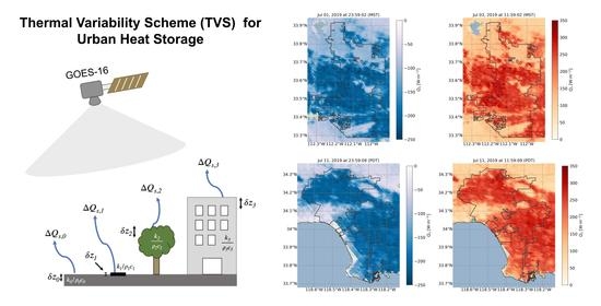
:Heat storage, , is quantified for 10 major U.S. cities using a method called the thermal variability scheme (TVS), which incorporates urban thermal mass parameters and the variability of land surface temperatures. The remotely sensed land surface temperature (LST) is retrieved from the GOES-16 satellite and is used in conjunction with high spatial resolution land cover and imperviousness classes. New York City is first used as a testing ground to compare the satellite-derived heat storage model to two other methods: a surface energy balance (SEB) residual derived from numerical weather model fluxes, and a residual calculated from ground-based eddy covariance flux tower measurements. The satellite determination of was found to fall between the residual method predicted by both the numerical weather model and the surface flux stations. The GOES-16 LST was then downscaled to 1-km using the WRF surface temperature output, which resulted in a higher spatial representation of storage heat in cities. The subsequent model was used to predict the total heat stored across 10 major urban areas across the contiguous United States for August 2019. The analysis presents a positive correlation between population density and heat storage, where higher density cities such as New York and Chicago have a higher capacity to store heat when compared to lower density cities such as Houston or Dallas. Application of the TVS ultimately has the potential to improve closure of the urban surface energy balance.
1. Introduction
Heat storage, , is defined as the uptake and release of energy by air, vegetation, buildings, and other impervious surfaces in an urban system [1,2]. The increase in both thermal conductivity and heat capacity is purported to amplify the total heat stored in cities above that of surrounding rural areas [3]. This net increase in is theorized as a major contributor to the urban heat island phenomenon—a widely recognized artifact of urbanization [4]. Furthermore, accurate estimation of urban heat storage is paramount for energy balance closure, which can have significant impacts on monitoring atmospheric processes such as evapotranspiration, transport of particulate matter, variations in sensible heat, and prediction of boundary layer height and stability [5].
Most often, the urban heat storage is determined as a residual of the surface energy balance (SEB) [6,7,8,9,10]. This is due to the use eddy covariance for computation of other flux terms in the SEB [11,12,13,14]. The second most common formulation of heat storage is the objective hysteresis model (OHM), which uses the temporal hysteresis of net all-wave radiation to relate the residual heat storage from the SEB to a given surface type [15,16]. A third method for computing involves a numerical model called the town energy balance (TEB). The TEB uses either the residual of the surface energy balance or the hysteresis model to formulate urban heat storage based on modeled fluxes [14,17,18]. Lastly, a fourth method can be found scattered throughout the literature and is based on a conduction and material storage model, referred to as both the element surface temperature method (ESTM) and the thermal mass scheme (TMS) [19,20,21,22].
Many studies have computed using surface observations, while very few have done so from the satellite perspective. In urban areas, the number of heat storage-related studies involving satellite observations is even lower [23]. This is likely due to the lack of standardization for computing heat storage, and the simultaneous difficulty of representing accurate fluxes from remotely-sensed imagery. One widely recognized satellite estimate of heat storage was computed using the residual method, which first computes every flux in the surface energy balance [24]. The element surface temperature method (ESTM) has gained popularity recently, perhaps due to increased computational power and numerical model capabilities [19,25]. However, the infrequency of satellite observations is still a clear hindrance on the ability to accurately characterize models associated with urban heat storage, as many of the satellite methods are unable to produce the full diurnal cycle of .
Long temporal overpass intervals have long been an obstacle for satellite applications. One recent advancement in the GOES-16 geostationary satellite allows snapshots of urban areas in the United States at spatial resolutions of 2 km every 5 min [26,27]. This high temporal resolution makes it the ideal candidate for implementing a thermal variability scheme (TVS) over urban areas. The TVS applied in this study is similar to a wide range of studies that estimate ground heat fluxes in soils using surface skin temperatures and material properties [28,29,30,31].
One of the more arduous tasks involved in deploying the TVS is the determination of the thermal mass of the urban fabric, i.e., the thermal conductivity, heat capacity, and material thickness [32]. Moreover, urban areas complicate things further by invalidating many of the established methods for deriving thermal properties due to the heterogeneous formation of buildings, roads, and other impervious land cover [33]. Consequently, the thermal properties of the satellite-derived urban heat storage employed here will be based on values determined in urban-specific studies aimed at quantifying the thermal mass of specific urban materials [34,35,36,37].
The resulting analytical, satellite-derived heat storage algorithm uses the 2-km land surface temperature (LST) outputted by the GOES-16 satellite, downscales it from 2 to 1 km, and uses its temporal hysteresis and the thermal masses of each land cover fraction to produce a 1-km spatial representation of urban heat storage. The development of the thermal variability scheme is similar to that of the thermal mass scheme and element surface temperature methods, which both use the variability of satellite-derived land surface temperature as an input to estimate heat storage. [19,38]. The TVS, as with other satellite routines, requires each satellite pixel to behave as a control volume element, which allows the surface energy balance to characterize each pixel as a unique portion of an urban area, allowing for partition of energy into components [39,40]. This is the general operating assumption of the thermal variability scheme as well.
These spatial constructions of are compared with ground-based flux towers and an urban weather research and forecasting (uWRF) model to determine its validity against two imperfect methods. The comparison is conducted for New York City during the summer of 2019, where all three data were available. The satellite model is ultimately extrapolated to the ten most populous cities in the United States and used to determine the variability of heat stored among different urban infrastructures. The development of the high temporal resolution satellite model has applications in investigating energy use, extreme heat impacts on vulnerable populations, and tracking pollution among increased urbanization [41]. Finally, the comparison between observations, numerical model, and satellite method will indicate where the deficit in closure of the surface energy balance, which may indicate that the numerical model could benefit from a restructuring of its prediction of heat storage in urban areas [42].
The aim of this study was to further the current understanding of the surface energy balance in urban areas, particularly with an innovative approach to determining heat stored in urban areas. Furthermore, the thermal variability scheme (TVS) developed using the GOES-16 satellite and publicly-available land cover information allow for heat storage to be calculated in all cities across the contiguous United States at a resolution of 1 km. The expectation is that this product will be used for urban surface energy balance studies whether through numerical models or comparison with surface flux stations, whether to determine other fluxes in the SEB or as a model for an improved estimate of heat storage.
2. Study Areas and Datasets
2.1. Test Site—New York City
New York City is used as a test site for estimating heat storage due to the availability of urban weather research and forecasting (uWRF) model runs and the presence of four surface flux towers within the boundaries of the city.
2.1.1. National Land Cover Database (NLCD)
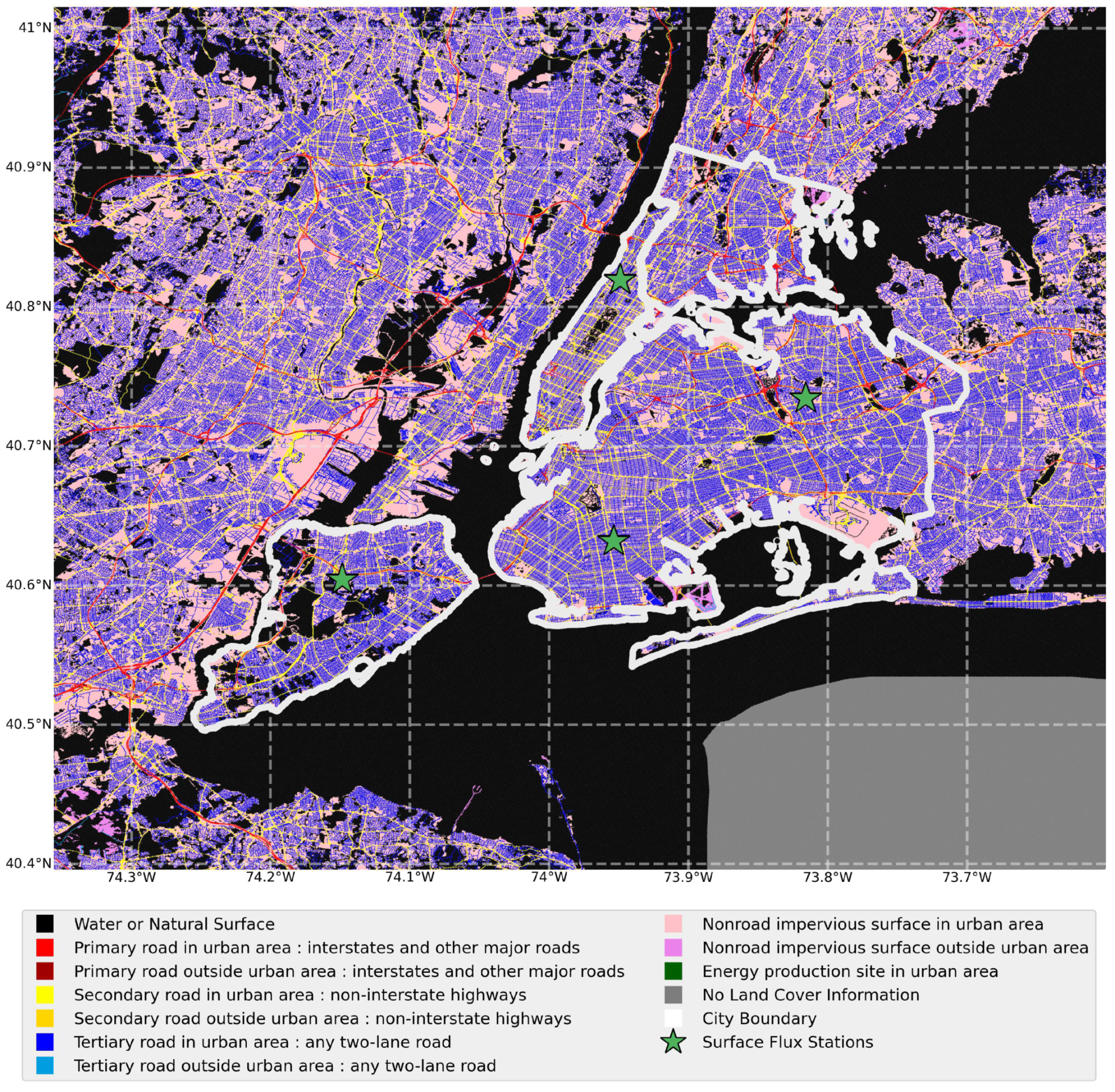
Figure 1 shows a map of New York City used for the analysis, with the National Land Cover Database (NLCD) 2016 imperviousness land cover categorization mapped atop the city’s boundary. Four green stars denote each surface flux station in Figure 1, which are used as comparison points in conjunction with the numerical WRF model. The NLCD 2016 is also being used to mask pixels that contain more than 30% water.
2.1.2. Surface Flux Stations
The New York State Mesonet (NYSMesonet) provides three of the four surface flux stations used as comparison points with the satellite-derived estimation of heat storage. The NYSMesonet uses Kipp and Zonen CNR4 net radiometers and a Campbell Scientific CPEC200 eddy covariance system that includes a 3D ultrasonic anemometer (CSAT3A) and closed-path gas analyzer (EC155) [43]. The fourth urban site is located at the City College of New York (CCNY) and uses a similar CSAT3 eddy covariance system by Campbell Scientific, and a CNR4 Kipp and Zonen net radiometer. The use of four close-proximity flux instruments allows for heat storage comparisons in four out of the five boroughs in New York City: Brooklyn, Manhattan, Queens, and Staten Island. The uniqueness of each station’s surface cover also aids in more accurately determining the validity of the satellite model.
The surface flux station data were available for the entire summer of 2019, courtesy of the NYSMesonet. The heat storage from the flux stations uses the residual heat storage between the net radiation and sensible and latent heat fluxes. The same is done for the weather research and forecasting model.
2.1.3. Weather Research and Forecasting Model (WRF)
The Weather Research and Forecasting (WRF) model is used as a second comparison point for the satellite heat storage algorithm. It is also used to downscale the land surface temperature output of the GOES-16 satellite from 2-km to a chosen WRF resolution of 1 km. The WRF model version 3.9.1.1 [44] is initialized with the North American Mesoscale (NAM) forecast and run for a series of dates in August 2019, using a spin-up time of 12 h for each run. Three nested domains were used for New York City, with spatial resolutions occupying 9 (120 × 120), 3 (121 × 121), and 1 (85 × 82). The vertical grid has 51 levels, with 30 levels confined to the boundary layer. The shortwave and longwave radiation schemes are the Dudhia scheme and the Rapid Radiative Transfer Model (RRTM) [45,46], respectively. The microphysics is activated only for the fine-grid 1-km domain using the WRF Single-moment, 6-class scheme [47]. For the land surface model, the NOAH scheme was used [48]. The Mellor–Yamada–Janjić and the Eta Similarity scheme were used for the boundary layer and surface layer schemes, respectively [49,50,51].
The large number of levels in the boundary-layer helps to better represent the building–atmosphere interaction within a multi-layer urban canopy framework. The coupled Building Environment Parameterization (BEP) and Building Energy Model (BEM) parameterize the urban surface momentum and thermal exchanges, respectively [52,53]. Each urban grid is subdivided into one of three urban land class categories: low-intensity residential, high-intensity residential, and commercial/industrial, and their properties are defined using a look-up table of urban canopy parameters from the National Urban Database and Access Portal Tool (NUDAPT) [54]. The standard BEP+BEM scheme, as described above, has been further modified to include two additions. First, a cooling tower model was added to the BEM parameterization to account for the latent heat released from buildings [55]. Second, for the urban grids in New York City, the Primary Land Use Tax Lot Output (PLUTO) was used to define the urban morphological parameters of building area fraction, building surface area-to-height ratio, and building heights, which then defined a mechanical drag coefficient. The PLUTO data have been aggregated from its tax lot-based resolution to 1-km aggregates for the fine resolution domain. Accounting for the mechanical and thermal effects of buildings has also resulted in more accurate estimates of urban temperatures and winds [56,57].
2.2. GOES-16 Land Surface Temperature
The GOES-16 land surface temperature (LST) used here is an enterprise algorithm produced at 5-min temporal intervals at a spatial resolution of 2-km across the contiguous United States (CONUS). LST values are derived using the infrared bands (band 14: 11.2 , and band 15: 12.3 ) and an approximation of emissivity using a daily split-window algorithm developed by the Land Surface Temperature Algorithm Working Group at the National Oceanic and Atmospheric Administration (NOAA) [58]. The enterprise LST product is selected over the baseline product due to the desired temporal resolution of 5 min vs. 1 h. This temporal improvement minimizes delays between comparisons between the satellite and the numerical model or surface flux stations. The enterprise LST product is only available to our team; however, the functional use of the heat storage method is applicable to the baseline product as well. Cloudy pixels were excluded from the analysis due to the cloud mask imposed by the LST product [27]. This is doubly detrimental to the estimation of due to the requirement of at least two LST values in Equation (8), which will decrease the availability of heat storage periodically throughout the analysis. There is also a land mask that nulls pixels near bodies of water based on sea level, which prevents contamination of sea surface on land surface temperatures.
2.3. Properties of the Ten Most Populous U.S. Cities
The ten most populous cities in the United States are listed in Table 1, with information about population, population density, and imperviousness percentage. The approximate area used for the analysis is not limited to the city boundaries; instead, it expands outward by roughly 10 km in each direction. This allows capture of the immediate urban area as well as some outer urbanization while also ensuring that no urban pixels are clipped during the analysis. This also increases the number of data points used in the analysis, which may be beneficial for smaller cities with few satellite pixels within the city boundaries.
The ten cities listed in Table 1 were chosen based on population, which are all above 1 million. The cities exhibit differing amounts of population density and imperviousness percentage. For example, New York, NY has a much denser population than Phoenix, AZ. Imperviousness is listed in Table 1 as it is a major component of the heat storage model presented here. The goal of comparing these ten cities is to gain insight into the possible relationship between urbanization or imperviousness and heat storage behavior. It has been hypothesized that heat storage may be the largest contributor to the urban heat island (UHI) effect, and the goal here is to determine if heat storage has any relation to increased urbanization or even the decrease of vegetation in some way contributing to UHI by way of increase storage of heat [8,61,62].
3. Methodology
3.1. Residual Heat Storage
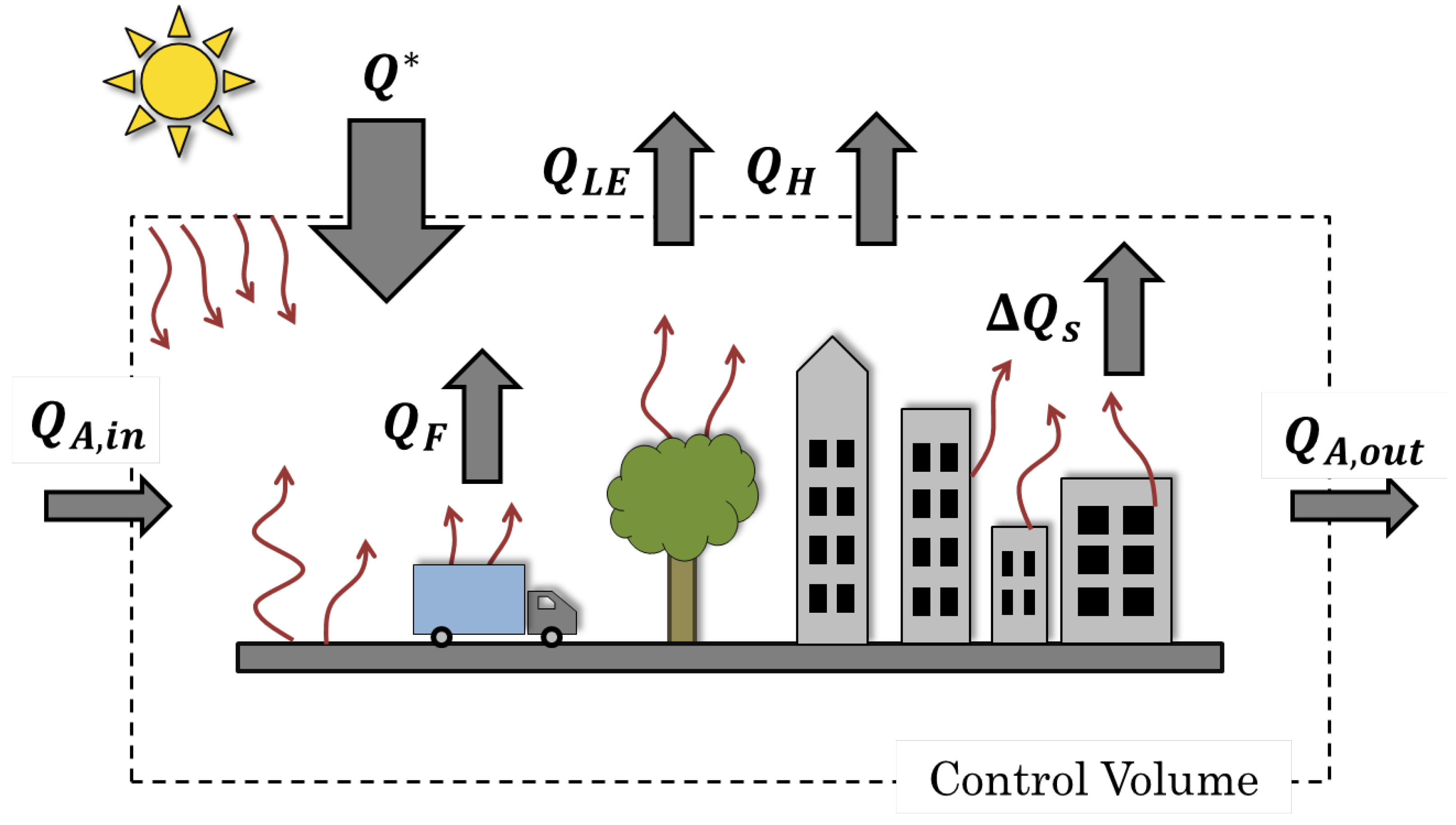
The surface energy balance (SEB) is often presented as the starting point for numerical weather models and meteorological observation studies interested in quantifying energetic processes within a given volumetric layer [4,63]. Figure 2 shows the balance of energetic components found in a typical urban control volume. The net all-wave radiation (), sensible heat flux (), latent heat flux (), and storage heat flux () are all included in the traditional surface energy balance, while the anthropogenic heat flux (), advective heat flux (), and other sources and sinks (S) are incorporated depending on their significance to a given application. The resulting surface energy balance for urban areas can be written as [64]:
where the external sources of energy are given on the left-hand side, and surface fluxes are given on the right-hand side [65]. The heat storage is often estimated as a residual to the surface energy balance in Equation (1), with varying degrees of components omitted. For many applications, is simplified as [6,7,23]:
This residual is used by both surface flux towers and the weather research and forecasting model to determine heat storage. For the particular case of a numerical model, the sensible heat flux captures much of the anthropogenic influence in the urban control volume. Flux stations are also considered to capture much of the anthropogenic influence in the sensible heat measurements. Thus, the prediction of from the satellite’s perspective will be compared with two approximations of heat storage that are assumed to account for to some degree [66].
3.2. Satellite Thermal Variability Scheme (TVS)
The satellite thermal variability scheme developed here determines heat storage from the perspective of the geostationary satellite. Its derivation begins where several analytical soil heat flux derivations begin: with the one-dimensional heat conduction equation [67,68,69]:
where represents the thermal conductivity, is the bulk density, and is the specific heat capacity, all of which are properties of the storage material. The storage of heat in a given material is written as a boundary condition on one-dimensional conduction at the surface, :
The second boundary condition imposed on the solution in the spatial domain invokes the assumption that at a certain depth in the material the temperature change with depth is negligible (adiabatic assumption) [70]:
The final condition implies that the temperature can be measured at two distinct points in time at the surface of material, , which allows the one-dimensional heat conduction equation to be solved-for. The solution and final storage representation arises from the solution based on the boundary conduction at the surface:
where is defined as:
The thermal diffusivity is defined here as . Two temperature measurements are required, , which are measured at times , respectively. This result is similar to those developed for determination of soil heat fluxes [71,72], with modifications for temporal measurements at the surface of the material. This result proposes that the amount of heat stored in a material can be determined using multiple surface temperature measurements and thermal properties of the storage material. This is a modification of the element surface temperature method and thermal mass schemes presented for a range of analyses [19,20,25].
One further adjustment need to be made in order to support multiple surface types within a given satellite pixel [64]:
where the plan area fraction, , defines each surface type’s contribution to the total heat stored within each satellite’s respective pixel. The index, i, represents the surface type within the array of total surface types, n. For the ensuing analysis, four different storage surface types are explored for urban areas: natural, buildings, roads, and other impervious surfaces. The different material properties will be explored in the next section, where values are sourced from comparable studies on thermal mass and heat storage.
3.3. Determination of Thermal Mass
Accurate determination of thermal mass is essential for estimating how much heat will be stored in a given urban fabric [19,73]. The various thermal properties of urban materials, i.e., the thermal conductivity and heat capacity, are widely available in the literature pertaining to building energy and building materials. Unfortunately, much of the urban landscape is comprised of an array of materials that differ in thicknesses and composition. This results in a characterization of thermal mass that introduces great uncertainty and reaffirms a commonly-held hypothesis that direct measurement or modeling of is nearly impossible [8,74].
For the satellite thermal variability approach to heat storage, three static material properties are needed according to Equation (8): thermal conductivity (k), heat capacity (), and effective thickness (). The two thermal properties are known for most building materials; however, at the satellite pixel scale of 1–2 km, lumped element properties are used in place of micro-scale building properties. This saves computation time as well as data requirements, as specific building material databases are generally not available at such large scales. The thickness of the material layer, , is perhaps the largest unknown due to varying methodologies around heat storage. As a starting point, values and ranges were taken from comparable studies, particularly those in [3,5,7,64]. The particular values used for the four surface types (natural, buildings, roads, and other impervious) were based on a sensitivity study comparing values with a numerical model and several surface flux stations. Table 2 shows the chosen values for thermal mass parameters that are used going forward for the estimation of .
Each GOES-16 satellite pixel is subdivided into land cover fraction, , using the most recent National Land Cover Database, the NLCD 2016. The NLCD is useful due to its widespread use in numerical weather modeling, environmental planning, and urban development [75]. The NLCD 2016 specifically contains 30-m land cover information for the United States based on 20 different land cover types, 4 of which are urban-specific [76]. The four urban classifications can be further expanded to 12 imperviousness categories, where roads and other impervious surfaces are distinguished from one another. This results in a classification for three out of the four storage fractions (): natural cover, roads, and other non-road impervious surfaces. Determination of the final surface type, buildings (), requires parameterization of the non-road imperviousness category.
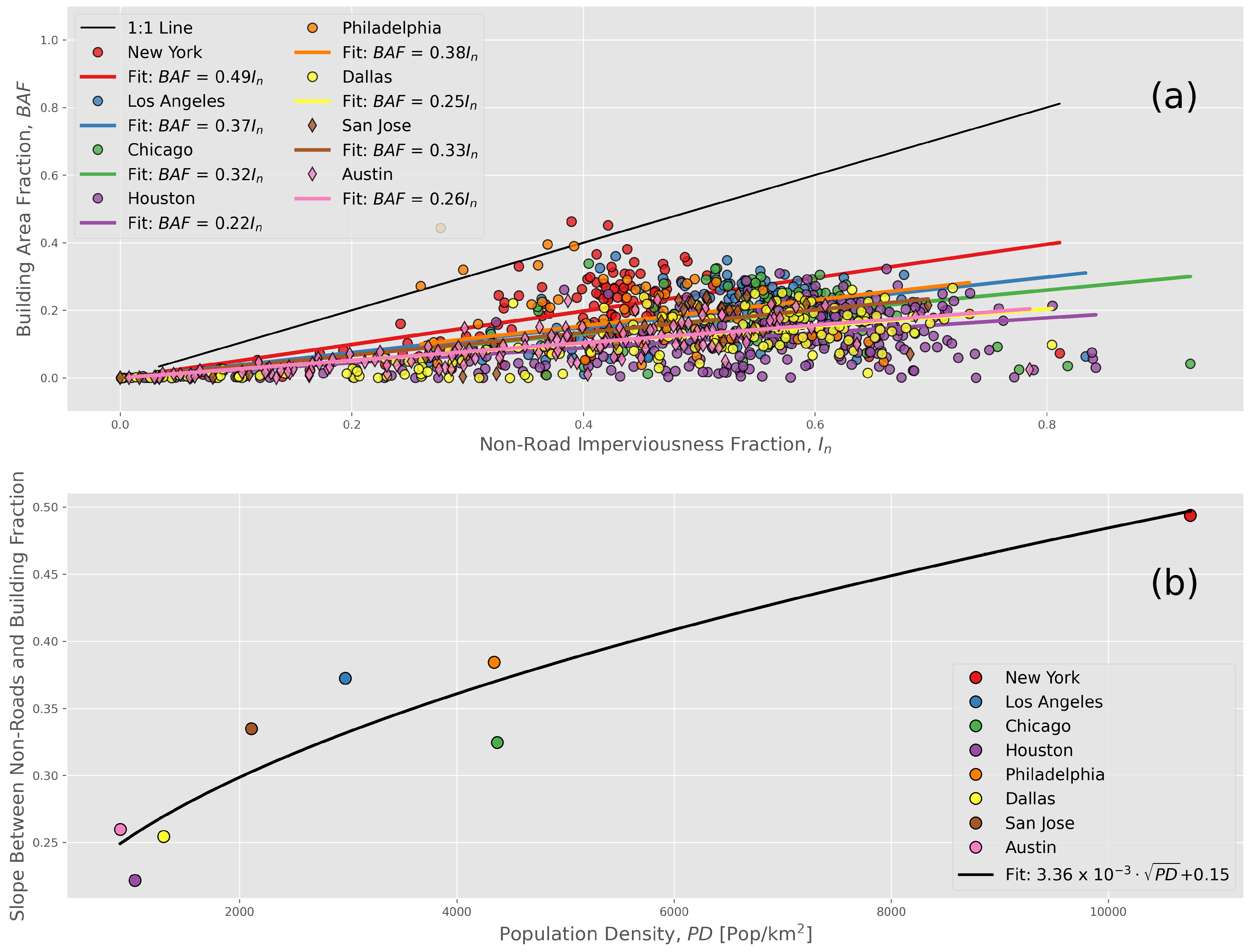
The fraction of buildings present in each satellite pixel was determined by first collecting building databases for eight out of eleven of the largest U.S. cities by population: New York, Los Angeles, Chicago, Houston, Philadelphia, Dallas, San Jose, and Austin. Three of the eleven were omitted due to lack of publicly available data. Figure 3a shows the relationship between building area fraction and non-road imperviousness land cover fraction. The points above the 1:1 line likely represent situations where the city developed buildings within the four years since the development of the NLCD 2016 product. A modest correlation exists between the square-root of population density and the slope between non-road imperviousness and building area fraction. This relationship can be written as follows:
where is an abbreviation for building area fraction, represents the corresponding satellite pixel’s non-road imperviousness fraction, is the population density, and a and b are the fit coefficients derived from the cities in Figure 3. This representation of building area fraction serves as the method for determining the thermal mass contribution of buildings to storage heat. This relationship is particularly useful for cities and outlying suburban regions where building databases are unavailable. With this parameterization of building area fraction derived from the NLCD’s non-road imperviousness fraction, the four components of the thermal mass are compiled for every city in the United States, completing the model and enabling comparison between heat storage for major U.S. cities.
3.4. Land Surface Temperature Downscaling
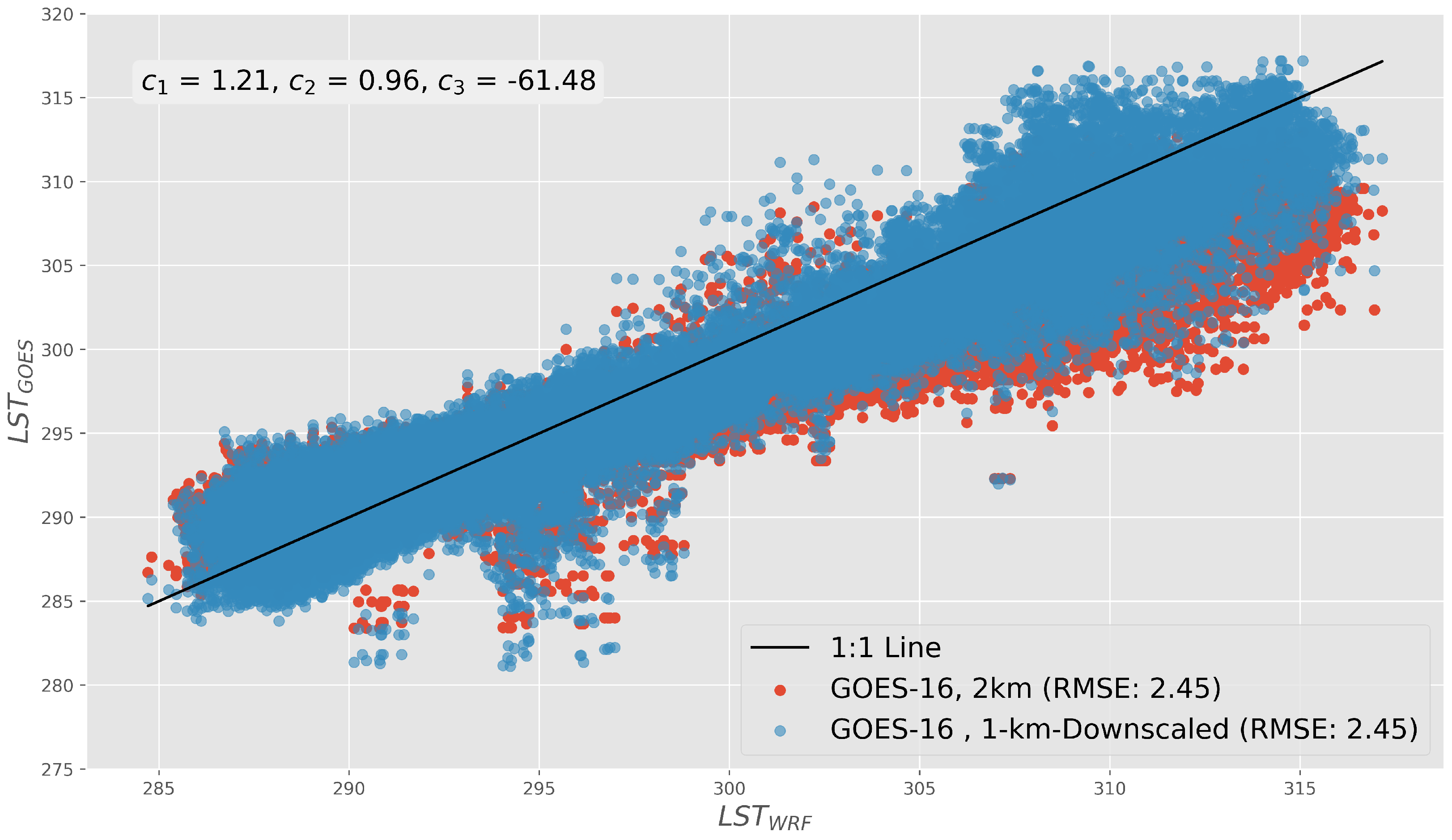
The land surface temperature (LST) used here is released as an enterprise dataset and has a temporal resolution of 5 min. The temporal capabilities of the enterprise product allows for comparisons down to just a few minutes between satellite LST and either ground observations or numerical model comparisons. The native spatial resolution for the GOES-16 land surface temperature is 2 km, which creates only a few dozen points within each urban boundary. This poor spatial resolution resulted in the decision to downscale the GOES-16 LST from 2 to 1 km. The weather research and forecasting (WRF) model’s LST is used as the comparison temperature for downscaling due to its 1-km spatial resolution and good agreement with other satellites [77]. The downscaling uses the imperviousness fraction based on the NLCD 2016, and follows the DisTrad method for downscaling the LST outlined in [78] and applied to urban areas by Essa et al. [79,80]. The resulting 1-km LST can be approximated using the following relationship:
where represents the 1-km LST value at index i. The coefficients, , are found using the least-squares fit between the WRF LST at 1 km and the GOES-16 LST at 2 km, as well as the respective imperviousness fraction at 1 km () and 2 km (), according to Equation (10). The subscript j denotes 2-km variables, while i denotes 1-km variables.
4. Results and Discussion
4.1. Case Study—New York City
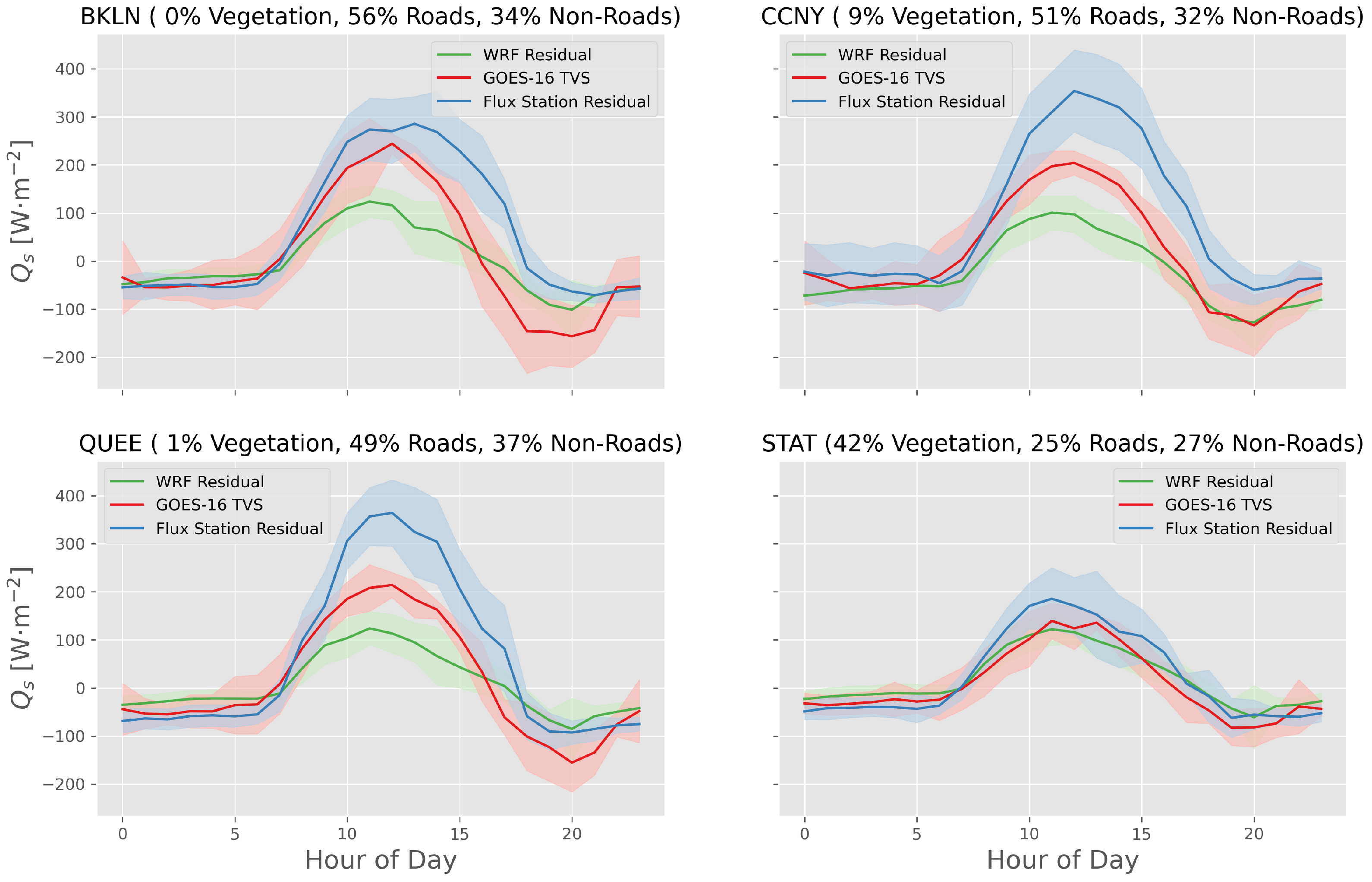
The satellite thermal variability scheme (TVS) estimate of heat storage at 2-km spatial resolution is first tested in New York City against four urban surface flux stations provided by the NYSMesonet and an urban Weather Research and Forecasting (uWRF) model. The nearest satellite and uWRF pixels were selected based on centroids located nearest to each ground station coordinate. Figure 4 shows the comparison between the three different estimates of heat storage. The satellite method uses an 8-h temporal difference, , between land surface temperature measurements in the prediction of . This was chosen based on minimizing the lag between satellite-derived storage and the other two residual methods while also ensuring that the difference between two temperature values is large enough to surpass the mission requirement error of 2.5K for the GOES-16 LST product [27].
One clear statement can be made regarding the comparison of satellite-derived, observed, and numerically modeled estimates of heat storage: the variability among them during the daytime. The surface flux stations appear to over predict in comparison with WRF and GOES-16 values. The WRF model is universally lower than both the GOES-16 approximation and satellite model.
One hypothesis for the lower heat storage capability of the WRF model is the inclusion of anthropogenic heat flux into the parameterization of sensible heat in the form of air conditioning and heat release from buildings [54,81]. Since WRF does not directly model , the resulting residual of the energy balance is offset by the larger value of . Similarly, the exclusion of advection and other sources to the residual energy balance of Equation (2) may also explain the higher amplitudes from flux station observations. The residual of the surface energy balance has long been a point of contention, and it is widely recognized to overestimate , due to either the aforementioned reasons or a combination of overestimates of and underestimates of [7,64,82,83]. This is perhaps an indication that the satellite-derived thermal mass estimate is closer to the real storage contribution of urban materials when compared to surface energy balance residuals derived by numerical models or flux observations.
4.2. Downscaling LST to 1 km
The coefficients are found using a three-day period in August 2019, with a least-squares fit between the WRF LST as the variable in Equation (10) and NLCD 2016 imperviousness as the inputs across New York City:
Figure 5 shows the performance improvement after downscaling LST from the GOES-16 satellite to the 1-km WRF resolution. It is important to note that the coefficients were found for a WRF run from 9 to 12 August 2019, while the data in Figure 5 were independently tested for those coefficients with a WRF run from 29 August to 1 September 2019. Furthermore, similar errors were presented by Bechtel et al. [84] for an urban study in Hamburg, Germany, where LST from the Spinning Enhanced Visible and Infrared Imager (SEVIRI) was downscaled from 1 km to 300 m using the Advanced Spaceborne Thermal Emission and Reflection Radiometer (ASTER).
4.3. One-Kilometer Heat Storage Comparison with uWRF
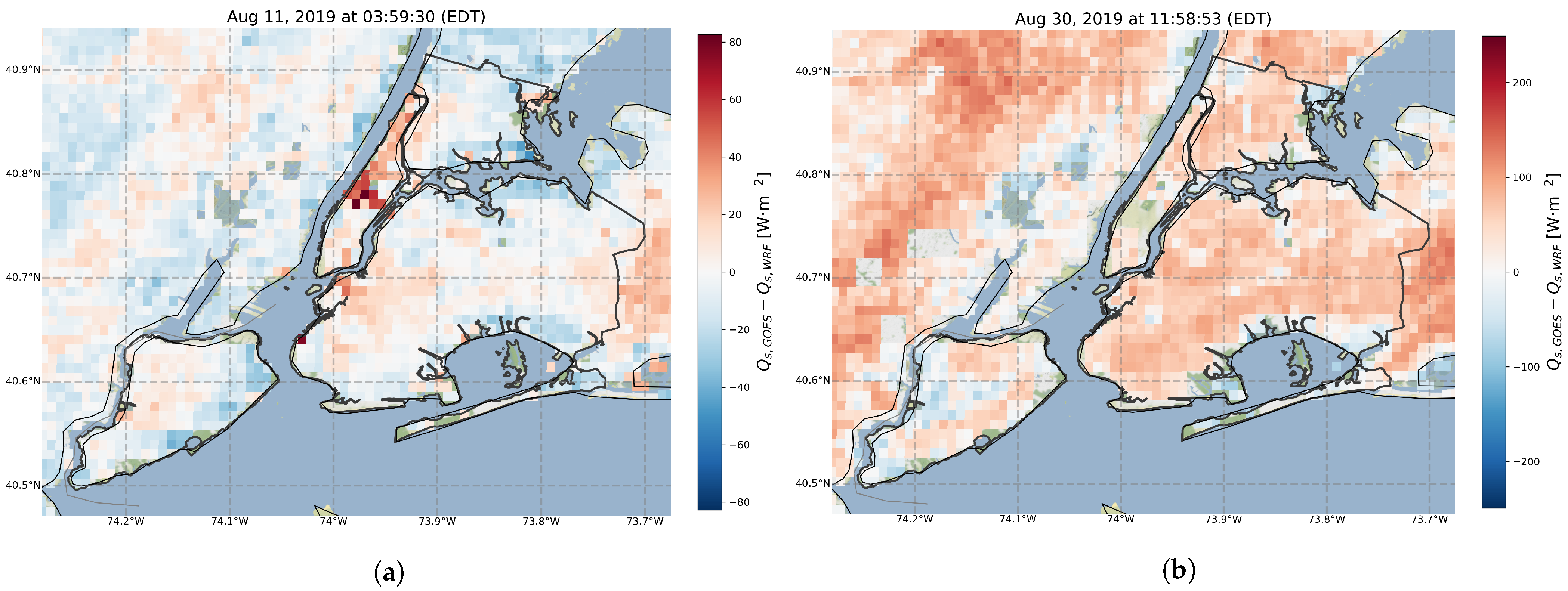
The native 2-km spatial resolution of land surface temperature produced by the GOES-16 satellite was used to validate the thermal variability scheme by generating similar profiles as the residual method for both the WRF model and surface eddy covariance observations. Unfortunately, many pixels are dropped and significant dynamics are obscured at the city scale due to coarseness in spatial resolution. As a result, the land surface temperature is downscaled to 1 km and used as input to the same determination of . The 1-km heat storage is used going forward for all spatial representations of . Figure 6 shows a 1-km spatial difference plot of heat storage during the daytime and nighttime in New York City, where the uWRF estimate has been subtracted from the GOES-16 estimate.
Several observations can be made regarding the difference between estimates of heat storage in Figure 6. First, in Figure 6a, the center of the city particularly shows a tendency toward higher storage from the satellite’s perspective. It is difficult to make any other distinctions between satellite and uWRF estimates, as there is a distribution of difference values scattered throughout the city. The mean absolute difference between satellite and numerical model during the nighttime agree quite well to within 15 Wm, indicating fairly good agreement throughout the city. This was also observed for the sites and pixels in Figure 4.
During the daytime in Figure 6b, the satellite model mostly dominates the numerical model. The difference plot shows higher heat storage along the coast for the uWRF estimate, which appears to be a result of the satellite method tending toward zero. This may be due to the influence of seabreeze, or perhaps an artifact of the satellite algorithm’s handling of land/water pixels. Several pockets within the city also appear to agree well for the daytime period, amounting to a mean absolute difference of 52 Wm, which is similar to other daytime comparisons between heat storage approximations [3,7,15].
The behavior exhibited in Figure 6 between the satellite method and numerical model are consistent across several days of observations. This affirms the findings in Figure 4, which shows that the satellite model differences are minimized during the nighttime and maximized during the daytime. A possible hypothesis is that if a 1-km spatial distribution of flux towers existed, the satellite estimation of would fall within the bounds of the uWRF model and flux tower amplitudes, particularly during the daytime. In the next section, the 1-km spatial representation of is presented and used for analyzing and comparing multiple cities and their ability to store heat.
4.4. Multi-City Analysis
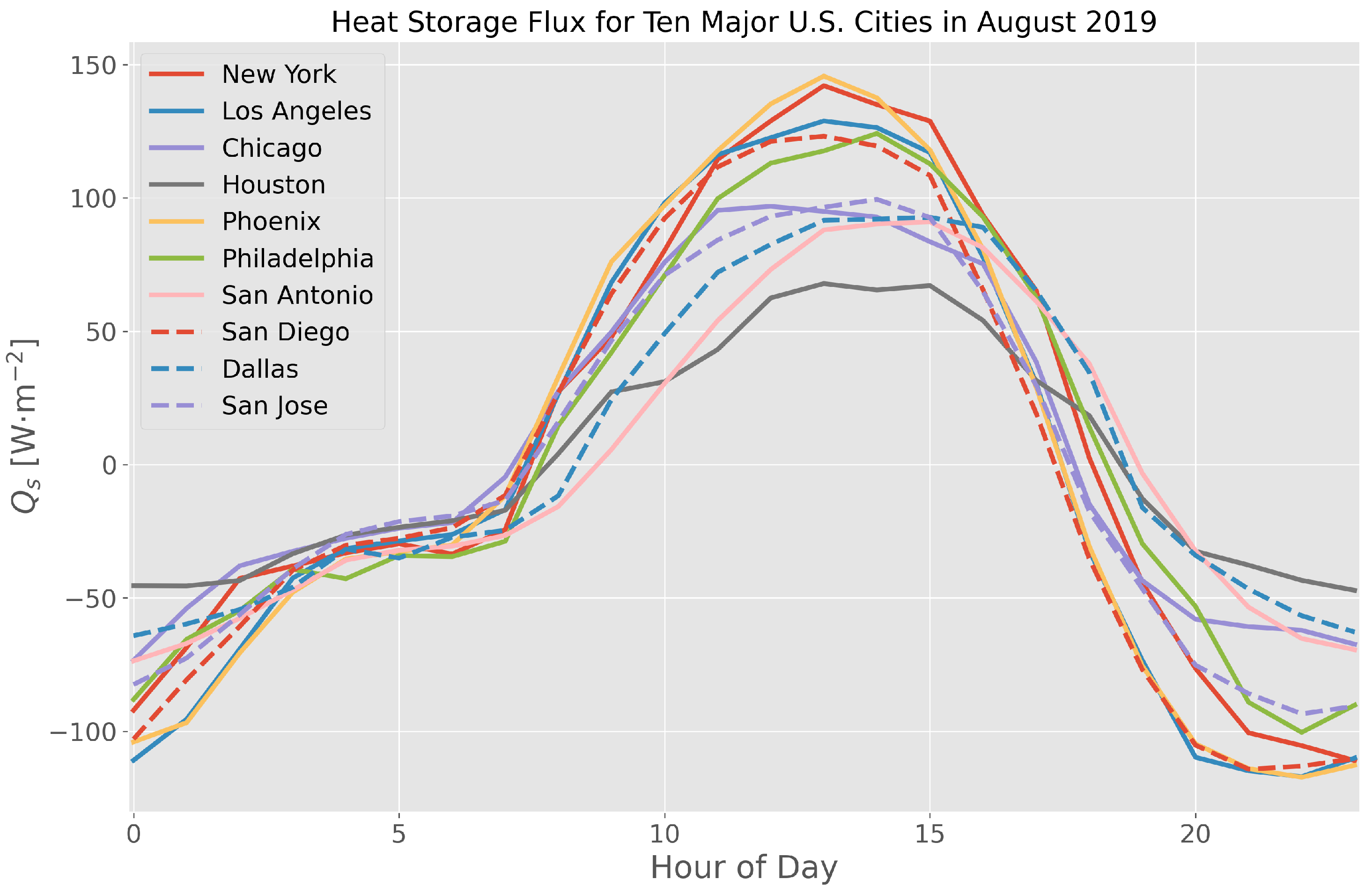
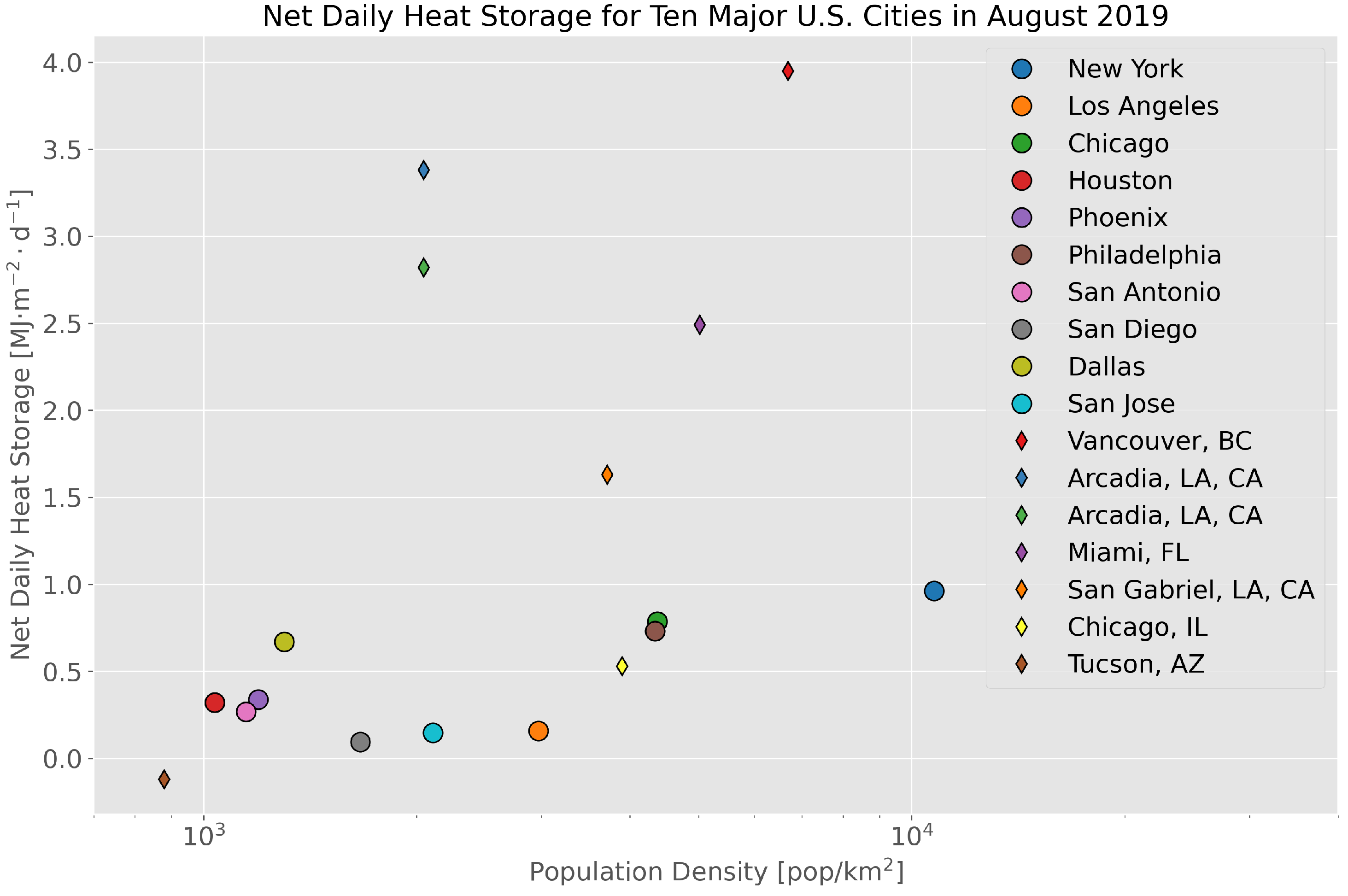
Heat storage is computed across the ten largest U.S. cities by population for the month of August 2019. Figure 7 shows the diurnal behavior of each city’s heat storage based on the satellite-derived thermal variability scheme (TVS). Upon integration of the amplitudes over the 24-h diurnal profile, an approximate value for daily heat storage flux for summertime can be found. This was done as a way of comparing the values with observations and models in the literature, as shown in Figure 8, where population density is plotted as a function of daily net heat storage. The range of values for suburban and urban areas can be found to fall between roughly −0.1 and 4.0 MJmday, which bookends the range observed in our analysis for August 2019 [1,9,85].
Two of the heat storage values from the literature (Tucson, AZ, USA and Chicago, IL, USA) fall directly inline with the approximations by the satellite model. The larger values taken from the literature in Figure 8 (Arcadia, CA, USA; Vancouver, BC, Canada; etc.) are likely evidence of a combination of anthropogenic influence, advection, and other sources that were also found to bias the New York City heat storage residuals in Figure 4.
The direct comparison between flux tower and satellite TVS may be inappropriate due to the limited footprint of the eddy covariance system. Depending on the characteristics of a particular site, the flux tower residual heat storage may or may not accurately represent the heat storage capabilities of the city as a whole [86,87,88]. This is perhaps why some of the stations match the satellite algorithm and others do not. Despite the outliers in comparison with surface stations, confidence has accumulated around the satellite TVS due to its stability and marginal agreement in amplitude with surface stations and previous studies. Consequently, a few spatial distributions of heat storage from the satellite’s perspective RE presented.
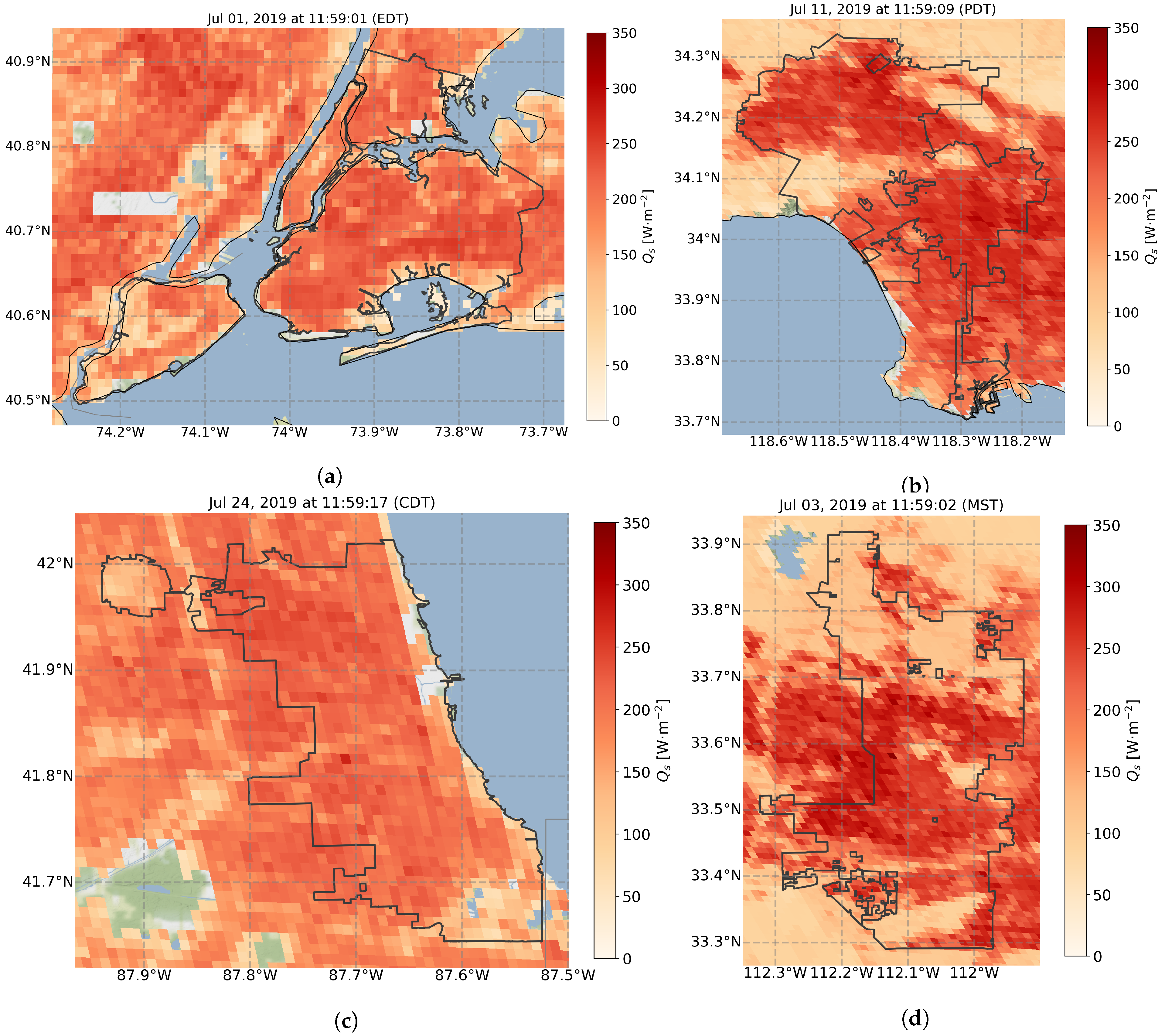
Figure 9 shows near-peak daytime heat storage from July 2019 plotted for four different cities: New York, Los Angeles, Phoenix, and Dallas. The cities were chosen in an attempt to diversify the urban microclimates without needing to produce individual plots for each of the ten cities referenced in Figure 7. New York was chosen for its humid subtropical climate, Los Angeles for its Mediterranean climate, Chicago for its continental climate, and Phoenix for its hot desert climate [89,90].
The peak values for each city align with each urban area, which is likely a result of the urban materials having higher thermal mass. Smaller storage values can be found around non-urban areas, as they have smaller thermal mass when compared to the nearby urban materials. Another perhaps less expected observation is that the coastal urban areas have lower storage values near water. Fortunately, similar observations of this mixed-pixel coastal behavior can be found in [19,91]. One possible explanation of the coastal storage aberration is the poor retrieval of LST around a mixed pixel or even the inability for the algorithm to downscale a water-contaminated pixel. Both New York and Chicago exhibit less variability between highly urban and less urban areas, whereas Los Angeles and Phoenix demonstrate larger fluctuations between urban and suburban/rural areas. This may be explained by the surrounding Mediterranean and desert climates, where a larger portion of the incident energy is released back into the atmosphere as sensible heat and the thermal mass values are smaller. Moreover, New York and Chicago also have more suburban regions within their boundaries in Figure 9 and Figure 10, which may also explain the lower variability between highly urbanized and less urbanized areas. Similar behavior was also observed by Middel et al. [92] for Phoenix, AZ.
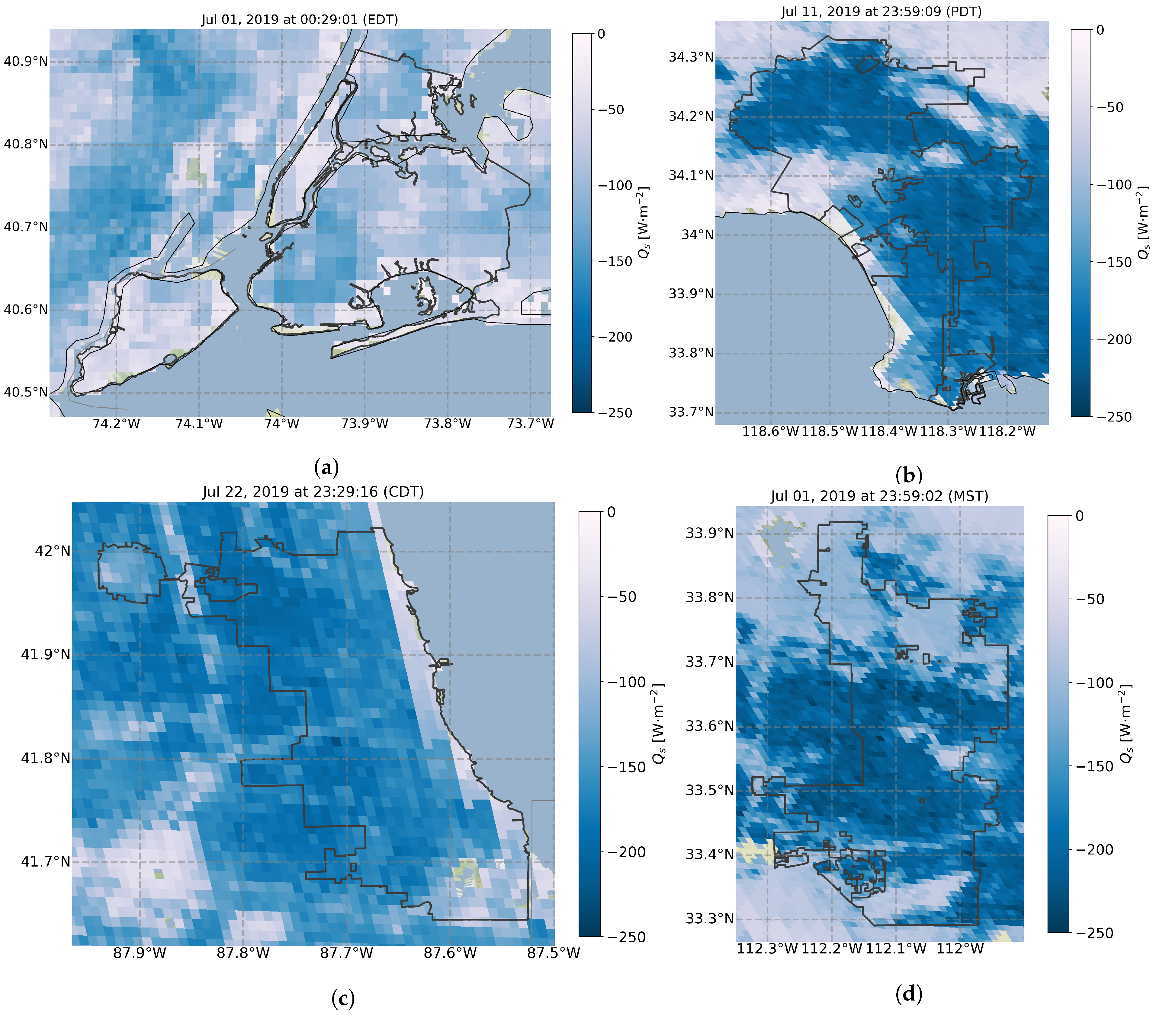
Figure 10 shows for the same four cities during the nighttime, which further exemplifies the unique behavior of heat storage in urban areas. Subplot Figure 10a shows the variability between heat storage during the nighttime, where New York City’s Central Park (center of plot) is seen releasing less heat compared to the more urban areas, particularly in downtown Manhattan and Brooklyn. Los Angeles during the nighttime experiences higher variability when compared to New York, with larger span between urban and rural storage values. The upper-right portion of Los Angeles is home to a national forest at higher elevation, which can be seen as having lower heat storage during the daytime and a more tempered release during the nighttime.
Chicago is similar to New York in that it is widely urban and suburban with little vegetation. Consequently, it experiences a more even distribution of heat storage, with the exception of a large park in the lower lefthand corner of Figure 10c.
Phoenix, in contrast to New York and Chicago, has a much higher release of heat storage during the nighttime. This can be observed in Figure 10d, where the blues are roughly as dark as Los Angeles, but much darker than New York and Chicago—indicating a more intense release of storage during the nighttime. This was also observed in the city-wide diurnal average, where Phoenix, Los Angeles, and San Diego all exhibited the largest release of storage heat for all ten major cities.
4.5. Discussion
One of the implications of the results presented here is the interpretation of current frameworks to estimate . Observations from eddy covariance methods show that the residual term, often used to represents , is very high compared to the WRF residual method. Our results show that the thermal variability scheme estimate of is within 60–70% of the residual term computed from the flux tower. This is partially due to the tuning of parameters in the diurnal comparison of values between satellite TVS, uWRF residual, and flux tower residual. There is a possibility that advection is a more prominent term in the Urban SEB than previously believedand that the lower TVS values may be further indication of such phenomena [93]. Furthermore, there is also a possibility that eddy covariance systems are incapable of capturing all energy-containing eddies in urban environments. The residual term is uniformly high at all three urban sites, as shown in Figure 4. Interestingly, in the least urban of the four sites, Staten Island (STAT) where the flux tower is located in a suburban environment with 42% vegetation cover, the values estimated by the TVS method match reasonably well with the residual term and numerical model. This bolsters the hypothesis that caution should be taken when representing as the residual term in the surface energy balance for highly urbanized sites. Previous studies that have elaborately used the residual strategy for determining may, in fact, be overestimating the storage heat term in urban areas. On the other hand, the numerical model exhibits lower values when compared to the satellite method, which may be related to the lack of parameterization for storage heat flux in the urban canopy models. Many researchers in the past have observed larger amplitudes in sensible heat flux predicted by numerical models in urban areas, resulting in a residual term with a lower amplitude. Urban canopy models are designed based on traditional land surface models created for non-urban environments, where the available energy is partitioned between sensible and latent heat fluxes that are dependent on soil properties and vegetation type [94,95]. This is true even for the urban WRF model presented as a comparison here. However, this binary mode appears deficient in urban areas as the contribution to latent heat flux is weak in highly urbanized environments, resulting in the over-prediction of sensible heat.
The satellite method also has its own set of limitations; currently, at the native resolution, we are unable to account for the three-dimensionality of the urban surface cover and representing shadow effects is currently not possible. However, downscaling the data using high-resolution satellite images from NASA’s MODIS or EcoStress could potentially aid in this effort. Furthermore, the complexity of urban structures and the reliance on a predetermined thicknesses both contribute to the uncertainty and unpredictability of the thermal properties used for the TVS method. Currently, there is no uniform database on thermal and physical properties of urban materials. Here, our cross comparisons with other surface stations in multiple cities reinforced the confidence in the methods and values used to estimate the thermal mass.
Our analysis also shows that the storage heat flux remains positive throughout the daytime for all 10 major cities with the average peak value between 75–150 Wm. The spatially averaged values dip below zero during the nighttime period, with peak release values between −50 and −110 Wm. The gradients present in Figure 9 and Figure 10 indicate hot-spots within the cities that could potentially play a significant role in maintaining high urban heat island intensity during the nighttimes [96]. In general, it is widely acknowledged that temperate mid-latitude cities experience high urban heat island intensity during the nighttime periods [97]. The thermal gradients can also initiate highly localized flows within the urban environment, hence increasing the magnitude of advective fluxes.
5. Conclusions
A novel satellite-based thermal variability scheme (TVS) was introduced as a method for estimating heat storage, , in urban areas. The TVS method uses four categorizations of thermal mass in conjunction with the temporal variability of land surface temperature to predict . The high temporal resolution of the GOES-16 satellite allows for complete reconstruction of the diurnal profile of heat storage in urban areas—something lacking in previous works relating to satellite-derived estimates of storage heat.
The resulting model of heat storage exhibited behaviors comparable to both an urban weather research and forecasting model and four different surface flux observations in New York City. The test case of NYC uncovered the discrepancy between forecasting model and surface flux tower observations of . The satellite-derived estimate of storage mostly fell between the flux tower and WRF estimates, particularly during the daytime. During the nighttime, the satellite model dominates over the other two methods, and the morning shows all three collapse and mostly agree with one another. The comparison between satellite model, surface flux observations, and numerical model helped build confidence in the satellite method and resulted in its application to ten different major cities across the United States.
Before carrying out spatial representations of , land surface temperatures were downscaled from 2 to 1 km. This allowed for more pixels to populate the urban areas and create a better illustration of how cities store heat. The 1-km downscaling is based on comparisons with the WRF numerical model and the DisTrad method that uses imperviousness cover to allow for country-wide downscaling to 1 km by utilizing the National Land Cover Database’s imperviousness fraction category.
Using the novel TVS method at 1-km spatial resolution, heat storage was computed across the ten most populous cities in United States. Each city exhibited different behavior based on urbanization, population density, and heterogeneity of land cover. The daily net heat storage for the month of August 2019 was compared with other studies and was found to agree well with other urban areas, even those outside the ten cities in our analysis.
Following the reasonable agreement with values in the literature, spatial plots were presented using the TVS method as a way of exploring the unique and novel behavior of heat storage across different urban microclimates. Spatial reconstructions in New York, Los Angeles, Chicago, and Phoenix all demonstrated the influence of urbanization on the amplitude and variability of storage heat flux. During the nighttime, each city tends to behave similar to their respective daytime observations. Chicago and New York exhibit more uniformly distributed estimates of throughout their urban boundaries. Conversely, Los Angeles and Phoenix experience more drastic changes between the urban and non-urban regions. During the evening just after sunset, a large portion of the stored heat is released back into the atmosphere across all cities.
In closing, the satellite-derived estimation of heat storage may prove to be a key element in closing the surface energy balance for urban areas. This unique method of determining is a step toward removing the non-storage components often neglected in residual estimates of storage. The two prevailing methods, the residual method and objective hysteresis model, both use an oversimplified energy balance, which results in the larger amplitudes seen in flux tower observations when compared with the satellite method and numerical weather model. Additionally, the thermal variability scheme also opens the door for better weather research and forecasting estimates of heat storage in cities, which could ultimately improve the distribution of energy in weather models that will ultimately increase the predictability of extreme heat events that plague our cities.
Author Contributions
Conceptualization, J.H. and P.R.; Data curation, J.H. and D.M.-V.; Formal analysis, J.H.; Funding acquisition, J.E.G.; Investigation, J.H.; Methodology, J.H. and P.R.; Project administration, P.R. and J.E.G.; Resources, P.R. and D.M.-V.; Software, J.H.; Supervision, J.E.G.; Validation, J.H.; Visualization, J.H.; Writing—original draft, J.H.; and Writing–review and editing, J.H., P.R., and David Melecio-Vazquez. All authors have read and agreed to the published version of the manuscript.
Funding
This study was supported and monitored by The National Oceanic and Atmospheric Administration – Cooperative Science Center for Earth System Sciences and Remote Sensing Technologies (NOAA-CESSRST) under the Cooperative Agreement Grant No. NA16SEC4810008. The authors thank The City College of New York, NOAA-CESSRST (aka CREST) program and NOAA Office of Education, Educational Partnership Program for full fellowship support for Joshua Hrisko. The statements contained within the manuscript/research article are not the opinions of the funding agency or the U.S. government, but reflect the authors’ opinions. The research was also funded by The Department of Defense Army Research Office Grant No. W911NF2020126. This research was also made possible by the New York State (NYS) Mesonet. Original funding for the NYS Mesonet was provided by Federal Emergency Management Agency grant FEMA-4085-DR-NY, with the continued support of the NYS Division of Homeland Security & Emergency Services; the state of New York; the Research Foundation for the State University of New York (SUNY); the University at Albany, SUNY; the Atmospheric Sciences Research Center (ASRC) at SUNY Albany; and the Department of Atmospheric and Environmental Sciences (DAES) at SUNY Albany.
Conflicts of Interest
The authors declare no conflict of interest. The funders had no role in the design of the study; in the collection, analyses, or interpretation of data; in the writing of the manuscript, or in the decision to publish the results.
References
- Grimmond, C.; Oke, T.R. Heat storage in urban areas: Local-scale observations and evaluation of a simple model. J. Appl. Meteorol. 1999, 38, 922–940. [Google Scholar] [CrossRef]
- Nunez, M.; Oke, T.R. The energy balance of an urban canyon. J. Appl. Meteorol. 1977, 16, 11–19. [Google Scholar] [CrossRef]
- Meyn, S.K.; Oke, T. Heat fluxes through roofs and their relevance to estimates of urban heat storage. Energy Build. 2009, 41, 745–752. [Google Scholar] [CrossRef] [Green Version]
- Oke, T.R. The urban energy balance. Prog. Phys. Geogr. 1988, 12, 471–508. [Google Scholar] [CrossRef]
- Lipson, M.J.; Hart, M.A.; Thatcher, M. Efficiently modelling urban heat storage: An interface conduction scheme in an urban land surface model (aTEB v2. 0). Geosci. Model Dev. 2017, 10, 991–1007. [Google Scholar] [CrossRef] [Green Version]
- Oke, T.; Cleugh, H. Urban heat storage derived as energy balance residuals. Bound.-Layer Meteorol. 1987, 39, 233–245. [Google Scholar] [CrossRef]
- Roberts, S.M.; Oke, T.R.; Grimmond, C.; Voogt, J.A. Comparison of four methods to estimate urban heat storage. J. Appl. Meteorol. Climatol. 2006, 45, 1766–1781. [Google Scholar] [CrossRef]
- Rizwan, A.M.; Dennis, L.Y.; Chunho, L. A review on the generation, determination and mitigation of Urban Heat Island. J. Environ. Sci. 2008, 20, 120–128. [Google Scholar] [CrossRef]
- Kawai, T.; Kanda, M. Urban energy balance obtained from the comprehensive outdoor scale model experiment. Part I: Basic features of the surface energy balance. J. Appl. Meteorol. Climatol. 2010, 49, 1341–1359. [Google Scholar] [CrossRef]
- Ferreira, M.J.; de Oliveira, A.P.; Soares, J. Diurnal variation in stored energy flux in São Paulo city, Brazil. Urban Clim. 2013, 5, 36–51. [Google Scholar] [CrossRef]
- Miao, S.; Dou, J.; Chen, F.; Li, J.; Li, A. Analysis of observations on the urban surface energy balance in Beijing. Sci. China Earth Sci. 2012, 55, 1881–1890. [Google Scholar] [CrossRef]
- Nordbo, A.; Järvi, L.; Vesala, T. Revised eddy covariance flux calculation methodologies–effect on urban energy balance. Tellus B Chem. Phys. Meteorol. 2012, 64, 18184. [Google Scholar] [CrossRef]
- Feigenwinter, C.; Vogt, R.; Christen, A. Eddy covariance measurements over urban areas. In Eddy Covariance; Springer: Berlin/Heidelberg, Germany, 2012; pp. 377–397. [Google Scholar] [CrossRef]
- Lemonsu, A.; Grimmond, C.; Masson, V. Modeling the surface energy balance of the core of an old Mediterranean city: Marseille. J. Appl. Meteorol. 2004, 43, 312–327. [Google Scholar] [CrossRef]
- Grimmond, C.; Cleugh, H.; Oke, T. An objective urban heat storage model and its comparison with other schemes. Atmos. Environ. Part B Urban Atmos. 1991, 25, 311–326. [Google Scholar] [CrossRef]
- Pearlmutter, D.; Berliner, P.; Shaviv, E. Evaluation of urban surface energy fluxes using an open-air scale model. J. Appl. Meteorol. 2005, 44, 532–545. [Google Scholar] [CrossRef]
- Masson, V. A physically-based scheme for the urban energy budget in atmospheric models. Bound.-Layer Meteorol. 2000, 94, 357–397. [Google Scholar] [CrossRef]
- Masson, V.; Grimmond, C.S.B.; Oke, T.R. Evaluation of the Town Energy Balance (TEB) scheme with direct measurements from dry districts in two cities. J. Appl. Meteorol. 2002, 41, 1011–1026. [Google Scholar] [CrossRef] [Green Version]
- Lindberg, F.; Olofson, K.; Sun, T.; Grimmond, C.; Feigenwinter, C. Urban storage heat flux variability explored using satellite, meteorological and geodata. Theor. Appl. Climatol. 2020, 141, 271–284. [Google Scholar] [CrossRef] [Green Version]
- Chrysoulakis, N.; Marconcini, M.; Gastellu-Etchegorry, J.P.; Grimmong, C.; Feigenwinter, C.; Lindberg, F.; Del Frate, F.; Klostermann, J.; Mi, Z.; Esch, T.; et al. Anthropogenic heat flux estimation from space. In Proceedings of the 2017 Joint Urban Remote Sensing Event (JURSE), Dubai, UAE, 6–8 March 2017; pp. 1–4. [Google Scholar] [CrossRef]
- Marconcini, M.; Heldens, W.; Del Frate, F.; Latini, D.; Mitraka, Z.; Lindberg, F. EO-based products in support of urban heat fluxes estimation. In Proceedings of the 2017 Joint Urban Remote Sensing Event (JURSE), Dubai, UAE, 6–8 March 2017; pp. 1–4. [Google Scholar] [CrossRef]
- Roberts, S.M.; Oke, T.; Voogt, J.; Grimmond, C.; Lemonsu, A. Energy storage in a european city center. In Proceedings of the Fifth International Conference on Urban Climate, Łódź, Poland, 1–5 September 2003. [Google Scholar]
- Rigo, G.; Parlow, E. Modelling the ground heat flux of an urban area using remote sensing data. Theor. Appl. Climatol. 2007, 90, 185–199. [Google Scholar] [CrossRef]
- Kato, S.; Yamaguchi, Y. Estimation of storage heat flux in an urban area using ASTER data. Remote Sens. Environ. 2007, 110, 1–17. [Google Scholar] [CrossRef]
- Chrysoulakis, N.; Grimmond, S.; Feigenwinter, C.; Lindberg, F.; Gastellu-Etchegorry, J.P.; Marconcini, M.; Mitraka, Z.; Stagakis, S.; Crawford, B.; Olofson, F.; et al. Urban energy exchanges monitoring from space. Sci. Rep. 2018, 8, 1–8. [Google Scholar] [CrossRef] [PubMed] [Green Version]
- Schmit, T.J.; Griffith, P.; Gunshor, M.M.; Daniels, J.M.; Goodman, S.J.; Lebair, W.J. A closer look at the ABI on the GOES-R series. Bull. Am. Meteorol. Soc. 2017, 98, 681–698. [Google Scholar] [CrossRef]
- Yu, Y.; Yu, P. Land Surface Temperature Product from the GOES-R Series. In The GOES-R Series; Elsevier: Amsterdam, The Netherlands, 2020; pp. 133–144. [Google Scholar] [CrossRef]
- Tsuang, B.J. Ground heat flux determination according to land skin temperature observations from in situ stations and satellites. J. Hydrometeorol. 2005, 6, 371–390. [Google Scholar] [CrossRef]
- van der Tol, C. Validation of remote sensing of bare soil ground heat flux. Remote Sens. Environ. 2012, 121, 275–286. [Google Scholar] [CrossRef]
- Verhoef, A.; Ottlé, C.; Cappelaere, B.; Murray, T.; Saux-Picart, S.; Zribi, M.; Maignan, F.; Boulain, N.; Demarty, J.; Ramier, D. Spatio-temporal surface soil heat flux estimates from satellite data; results for the AMMA experiment at the Fakara (Niger) supersite. Agric. For. Meteorol. 2012, 154, 55–66. [Google Scholar] [CrossRef] [Green Version]
- Liang, X.; Wood, E.F.; Lettenmaier, D.P. Modeling ground heat flux in land surface parameterization schemes. J. Geophys. Res. Atmos. 1999, 104, 9581–9600. [Google Scholar] [CrossRef]
- Murray, T.; Verhoef, A. Moving towards a more mechanistic approach in the determination of soil heat flux from remote measurements: I. A universal approach to calculate thermal inertia. Agric. For. Meteorol. 2007, 147, 80–87. [Google Scholar] [CrossRef]
- Eusuf, M.A.; Kassim, J. A Study on the Solar Energy Storage in Urban Materials and their Effects on Surface Temperature in Two Latitudes; ITEE: St. Lucia, Australia, 2005; p. 721. [Google Scholar]
- Takebayashi, H.; Moriyama, M. Study on surface heat budget of various pavements for urban heat island mitigation. Adv. Mater. Sci. Eng. 2012, 2012. [Google Scholar] [CrossRef] [Green Version]
- Sharaf, F. The impact of thermal mass on building energy consumption: A case study in Al Mafraq city in Jordan. Cogent Eng. 2020, 7, 1804092. [Google Scholar] [CrossRef]
- Zeng, R.; Wang, X.; Di, H.; Jiang, F.; Zhang, Y. New concepts and approach for developing energy efficient buildings: Ideal specific heat for building internal thermal mass. Energy Build. 2011, 43, 1081–1090. [Google Scholar] [CrossRef]
- Di Perna, C.; Stazi, F.; Casalena, A.U.; D’orazio, M. Influence of the internal inertia of the building envelope on summertime comfort in buildings with high internal heat loads. Energy Build. 2011, 43, 200–206. [Google Scholar] [CrossRef]
- Chen, G.; Wang, D.; Wang, Q.; Li, Y.; Wang, X.; Hang, J.; Gao, P.; Ou, C.; Wang, K. Scaled outdoor experimental studies of urban thermal environment in street canyon models with various aspect ratios and thermal storage. Sci. Total Environ. 2020, 726, 138147. [Google Scholar] [CrossRef] [PubMed]
- Peng, S.; Piao, S.; Ciais, P.; Friedlingstein, P.; Ottle, C.; Bréon, F.M.; Nan, H.; Zhou, L.; Myneni, R.B. Surface urban heat island across 419 global big cities. Environ. Sci. Technol. 2012, 46, 696–703. [Google Scholar] [CrossRef] [PubMed]
- Liu, W.; Feddema, J.; Hu, L.; Zung, A.; Brunsell, N. Seasonal and diurnal characteristics of land surface temperature and major explanatory factors in Harris County, Texas. Sustainability 2017, 9, 2324. [Google Scholar] [CrossRef] [Green Version]
- Taha, H. Modifying a mesoscale meteorological model to better incorporate urban heat storage: A bulk-parameterization approach. J. Appl. Meteorol. 1999, 38, 466–473. [Google Scholar] [CrossRef]
- Mirzaei, P.A.; Haghighat, F. Approaches to study urban heat island–abilities and limitations. Build. Environ. 2010, 45, 2192–2201. [Google Scholar] [CrossRef]
- NYS Mesonet. Flux Network, Downloaded. 2020. Available online: http://www.nysmesonet.org/networks/flux#stid=flux_voor (accessed on 2 October 2020).
- Skamarock, W.C.; Klemp, J.B.; Dudhia, J.; Gill, D.O.; Barker, D.M.; Duda, M.G.; Huang, X.Y.; Wang, W.; Powers, J.G. A Description of the Advanced Research WRF Version 3; NCAR Tech. Note NCAR/TN-475+ STR; Citeseer, 2008; pp. 1–125. Available online: https://opensky.ucar.edu/islandora/object/technotes:500 (accessed on 2 October 2020). [CrossRef]
- Dudhia, J. Numerical study of convection observed during the winter monsoon experiment using a mesoscale two-dimensional model. J. Atmos. Sci. 1989, 46, 3077–3107. [Google Scholar] [CrossRef]
- Mlawer, E.J.; Taubman, S.J.; Brown, P.D.; Iacono, M.J.; Clough, S.A. Radiative transfer for inhomogeneous atmospheres: RRTM, a validated correlated-k model for the longwave. J. Geophys. Res. Atmos. 1997, 102, 16663–16682. [Google Scholar] [CrossRef] [Green Version]
- Hong, S.Y.; Lim, J.O.J. The WRF single-moment 6-class microphysics scheme (WSM6). Asia-Pac. J. Atmos. Sci. 2006, 42, 129–151. [Google Scholar]
- Tewari, M.; Chen, F.; Wang, W.; Dudhia, J.; LeMone, M.; Mitchell, K.; Ek, M.; Gayno, G.; Wegiel, J.; Cuenca, R.; et al. Implementation and verification of the unified NOAH land surface model in the WRF model. In Proceedings of the 20th Conference on Weather Analysis and Forecasting/16th Conference on Numerical Weather Prediction; American Meteorological Society: Seattle, WA, USA, 2004; Volume 1115, pp. 1–6. [Google Scholar]
- Janjić, Z.I. The step-mountain eta coordinate model: Further developments of the convection, viscous sublayer, and turbulence closure schemes. Mon. Weather Rev. 1994, 122, 927–945. [Google Scholar] [CrossRef] [Green Version]
- Janjić, Z.I. Nonsingular implementation of the Mellor-Yamada level 2.5 scheme in the NCEP Meso model. NCEP Off. Note 2001, 437, 61. [Google Scholar]
- Monin, A.S.; Obukhov, A.M. Basic laws of turbulent mixing in the surface layer of the atmosphere. Contrib. Geophys. Inst. Acad. Sci. USSR 1954, 151, e187. [Google Scholar]
- Martilli, A.; Clappier, A.; Rotach, M.W. An urban surface exchange parameterisation for mesoscale models. Bound.-Layer Meteorol. 2002, 104, 261–304. [Google Scholar] [CrossRef]
- Salamanca, F.; Martilli, A. A new building energy model coupled with an urban canopy parameterization for urban climate simulations—Part II. Validation with one dimension off-line simulations. Theor. Appl. Climatol. 2010, 99, 345. [Google Scholar] [CrossRef]
- Chen, F.; Kusaka, H.; Bornstein, R.; Ching, J.; Grimmond, C.; Grossman-Clarke, S.; Loridan, T.; Manning, K.W.; Martilli, A.; Miao, S.; et al. The integrated WRF/urban modelling system: Development, evaluation, and applications to urban environmental problems. Int. J. Climatol. 2011, 31, 273–288. [Google Scholar] [CrossRef]
- Gutiérrez, E.; Martilli, A.; Santiago, J.; González, J. A mechanical drag coefficient formulation and urban canopy parameter assimilation technique for complex urban environments. Bound.-Layer Meteorol. 2015, 157, 333–341. [Google Scholar] [CrossRef]
- Yu, M.; González, J.; Miao, S.; Ramamurthy, P. On the Assessment of a Cooling Tower Scheme for High-Resolution Numerical Weather Modeling for Urban Areas. J. Appl. Meteorol. Climatol. 2019, 58, 1399–1415. [Google Scholar] [CrossRef]
- Yu, M.; González, J.; Miao, S. Evaluation of a mechanical drag coefficient formulation in the complex urban area of Beijing. Theor. Appl. Climatol. 2020, 142, 743–749. [Google Scholar] [CrossRef]
- Hrisko, J.; Ramamurthy, P.; Yu, Y.; Yu, P.; Melecio-Vázquez, D. Urban air temperature model using GOES-16 LST and a diurnal regressive neural network algorithm. Remote Sens. Environ. 2020, 237, 111495. [Google Scholar] [CrossRef]
- Centers for Disease Control and Prevention. 500 Cities: City Boundaries. Available online: https://chronicdata.cdc.gov/500-Cities/500-Cities-City-Boundaries/n44h-hy2j (accessed on 2 October 2020).
- U.S. Census Bureau. City and Town Population Totals: 2010–2019. Available online: https://www.census.gov/data/tables/time-series/demo/popest/2010s-total-cities-and-towns.html (accessed on 3 October 2020).
- Gallo, K.; McNab, A.; Karl, T.R.; Brown, J.F.; Hood, J.; Tarpley, J. The use of a vegetation index for assessment of the urban heat island effect. Remote Sens. 1993, 14, 2223–2230. [Google Scholar] [CrossRef]
- Saitoh, T.; Shimada, T.; Hoshi, H. Modeling and simulation of the Tokyo urban heat island. Atmos. Environ. 1996, 30, 3431–3442. [Google Scholar] [CrossRef]
- Grimmond, C.S.B.; Blackett, M.; Best, M.; Barlow, J.; Baik, J.; Belcher, S.; Bohnenstengel, S.; Calmet, I.; Chen, F.; Dandou, A.; et al. The international urban energy balance models comparison project: First results from phase 1. J. Appl. Meteorol. Climatol. 2010, 49, 1268–1292. [Google Scholar] [CrossRef]
- Offerle, B.; Grimmond, C.S.B.; Fortuniak, K. Heat storage and anthropogenic heat flux in relation to the energy balance of a central European city centre. Int. J. Climatol. A J. R. Meteorol. Soc. 2005, 25, 1405–1419. [Google Scholar] [CrossRef]
- Masson, V. Urban surface modeling and the meso-scale impact of cities. Theor. Appl. Climatol. 2006, 84, 35–45. [Google Scholar] [CrossRef]
- Kato, S.; Yamaguchi, Y. Analysis of urban heat-island effect using ASTER and ETM+ Data: Separation of anthropogenic heat discharge and natural heat radiation from sensible heat flux. Remote Sens. Environ. 2005, 99, 44–54. [Google Scholar] [CrossRef]
- Heusinkveld, B.G.; Jacobs, A.; Holtslag, A.; Berkowicz, S. Surface energy balance closure in an arid region: Role of soil heat flux. Agric. For. Meteorol. 2004, 122, 21–37. [Google Scholar] [CrossRef]
- Wang, Z.H.; Bou-Zeid, E. A novel approach for the estimation of soil ground heat flux. Agric. For. Meteorol. 2012, 154, 214–221. [Google Scholar] [CrossRef]
- Bennett, W.B.; Wang, J.; Bras, R.L. Estimation of global ground heat flux. J. Hydrometeorol. 2008, 9, 744–759. [Google Scholar] [CrossRef]
- Wang, Z.H. Reconstruction of soil thermal field from a single depth measurement. J. Hydrol. 2012, 464, 541–549. [Google Scholar] [CrossRef]
- Van Wijk, W.R.; De Vries, D. Periodic temperature variations in a homogeneous soil. Phys. Plant Environ. 1963, 1, 103–143. [Google Scholar]
- Holmes, T.; Owe, M.; De Jeu, R.; Kooi, H. Estimating the soil temperature profile from a single depth observation: A simple empirical heatflow solution. Water Resour. Res. 2008, 44. [Google Scholar] [CrossRef] [Green Version]
- Arnfield, A.J.; Grimmond, C. An urban canyon energy budget model and its application to urban storage heat flux modeling. Energy Build. 1998, 27, 61–68. [Google Scholar] [CrossRef]
- Christen, A.; Vogt, R. Energy and radiation balance of a central European city. Int. J. Climatol. A J. R. Meteorol. Soc. 2004, 24, 1395–1421. [Google Scholar] [CrossRef]
- Jin, S.; Homer, C.; Yang, L.; Danielson, P.; Dewitz, J.; Li, C.; Zhu, Z.; Xian, G.; Howard, D. Overall methodology design for the United States national land cover database 2016 products. Remote Sens. 2019, 11, 2971. [Google Scholar] [CrossRef] [Green Version]
- Yang, L.; Jin, S.; Danielson, P.; Homer, C.; Gass, L.; Bender, S.M.; Case, A.; Costello, C.; Dewitz, J.; Fry, J.; et al. A new generation of the United States National Land Cover Database: Requirements, research priorities, design, and implementation strategies. ISPRS J. Photogramm. Remote Sens. 2018, 146, 108–123. [Google Scholar] [CrossRef]
- Ramamurthy, P.; Li, D.; Bou-Zeid, E. High-resolution simulation of heatwave events in New York City. Theor. Appl. Climatol. 2017, 128, 89–102. [Google Scholar] [CrossRef]
- Kustas, W.P.; Norman, J.M.; Anderson, M.C.; French, A.N. Estimating subpixel surface temperatures and energy fluxes from the vegetation index–radiometric temperature relationship. Remote Sens. Environ. 2003, 85, 429–440. [Google Scholar] [CrossRef]
- Essa, W.; Verbeiren, B.; van der Kwast, J.; Van de Voorde, T.; Batelaan, O. Evaluation of the DisTrad thermal sharpening methodology for urban areas. Int. J. Appl. Earth Obs. Geoinf. 2012, 19, 163–172. [Google Scholar] [CrossRef]
- Essa, W.; van der Kwast, J.; Verbeiren, B.; Batelaan, O. Downscaling of thermal images over urban areas using the land surface temperature–impervious percentage relationship. Int. J. Appl. Earth Obs. Geoinf. 2013, 23, 95–108. [Google Scholar] [CrossRef]
- Salamanca, F.; Martilli, A.; Tewari, M.; Chen, F. A study of the urban boundary layer using different urban parameterizations and high-resolution urban canopy parameters with WRF. J. Appl. Meteorol. Climatol. 2011, 50, 1107–1128. [Google Scholar] [CrossRef]
- Moriwaki, R.; Kanda, M. Seasonal and diurnal fluxes of radiation, heat, water vapor, and carbon dioxide over a suburban area. J. Appl. Meteorol. 2004, 43, 1700–1710. [Google Scholar] [CrossRef]
- Wilson, K.; Goldstein, A.; Falge, E.; Aubinet, M.; Baldocchi, D.; Berbigier, P.; Bernhofer, C.; Ceulemans, R.; Dolman, H.; Field, C.; et al. Energy balance closure at FLUXNET sites. Agric. For. Meteorol. 2002, 113, 223–243. [Google Scholar] [CrossRef] [Green Version]
- Bechtel, B.; Zakšek, K.; Hoshyaripour, G. Downscaling land surface temperature in an urban area: A case study for Hamburg, Germany. Remote Sens. 2012, 4, 3184–3200. [Google Scholar] [CrossRef] [Green Version]
- Oke, T.R.; Spronken-Smith, R.; Jáuregui, E.; Grimmond, C.S. The energy balance of central Mexico City during the dry season. Atmos. Environ. 1999, 33, 3919–3930. [Google Scholar] [CrossRef]
- Gioli, B.; Miglietta, F.; De Martino, B.; Hutjes, R.W.; Dolman, H.A.; Lindroth, A.; Schumacher, M.; Sanz, M.J.; Manca, G.; Peressotti, A.; et al. Comparison between tower and aircraft-based eddy covariance fluxes in five European regions. Agric. For. Meteorol. 2004, 127, 1–16. [Google Scholar] [CrossRef]
- Bai, J.; Jia, L.; Liu, S.; Xu, Z.; Hu, G.; Zhu, M.; Song, L. Characterizing the footprint of eddy covariance system and large aperture scintillometer measurements to validate satellite-based surface fluxes. IEEE Geosci. Remote Sens. Lett. 2015, 12, 943–947. [Google Scholar] [CrossRef]
- Jung, M.; Reichstein, M.; Margolis, H.A.; Cescatti, A.; Richardson, A.D.; Arain, M.A.; Arneth, A.; Bernhofer, C.; Bonal, D.; Chen, J.; et al. Global patterns of land-atmosphere fluxes of carbon dioxide, latent heat, and sensible heat derived from eddy covariance, satellite, and meteorological observations. J. Geophys. Res. Biogeosciences 2011, 116. [Google Scholar] [CrossRef] [Green Version]
- Wang, C.; Li, Y.; Myint, S.W.; Zhao, Q.; Wentz, E.A. Impacts of spatial clustering of urban land cover on land surface temperature across Köppen climate zones in the contiguous United States. Landsc. Urban Plan. 2019, 192, 103668. [Google Scholar] [CrossRef]
- Tewari, M.; Yang, J.; Kusaka, H.; Salamanca, F.; Watson, C.; Treinish, L. Interaction of urban heat islands and heat waves under current and future climate conditions and their mitigation using green and cool roofs in New York City and Phoenix, Arizona. Environ. Res. Lett. 2019, 14, 034002. [Google Scholar] [CrossRef]
- Hrisko, J.; Ramamurthy, P.; Gonzalez, J.E. Estimating heat storage in urban areas using multispectral satellite data and machine learning. Remote. Sens. Environ. 2021, 252, 112125. [Google Scholar] [CrossRef]
- Middel, A.; Brazel, A.J.; Kaplan, S.; Myint, S.W. Daytime cooling efficiency and diurnal energy balance in Phoenix, Arizona, USA. Clim. Res. 2012, 54, 21–34. [Google Scholar] [CrossRef] [Green Version]
- Xu, Z.; Ma, Y.; Liu, S.; Shi, W.; Wang, J. Assessment of the energy balance closure under advective conditions and its impact using remote sensing data. J. Appl. Meteorol. Climatol. 2017, 56, 127–140. [Google Scholar] [CrossRef]
- Nemunaitis-Berry, K.L.; Klein, P.M.; Basara, J.B.; Fedorovich, E. Sensitivity of predictions of the urban surface energy balance and heat island to variations of urban canopy parameters in simulations with the WRF Model. J. Appl. Meteorol. Climatol. 2017, 56, 573–595. [Google Scholar] [CrossRef] [Green Version]
- Pan, H.L.; Mahrt, L. Interaction between soil hydrology and boundary-layer development. Bound.-Layer Meteorol. 1987, 38, 185–202. [Google Scholar] [CrossRef]
- Zhou, J.; Chen, Y.; Wang, J.; Zhan, W. Maximum nighttime urban heat island (UHI) intensity simulation by integrating remotely sensed data and meteorological observations. IEEE J. Sel. Top. Appl. Earth Obs. Remote Sens. 2010, 4, 138–146. [Google Scholar] [CrossRef]
- Mihalakakou, G.; Santamouris, M.; Papanikolaou, N.; Cartalis, C.; Tsangrassoulis, A. Simulation of the urban heat island phenomenon in Mediterranean climates. Pure Appl. Geophys. 2004, 161, 429–451. [Google Scholar] [CrossRef]
Figure 1.
Imperviousness land cover from NLCD 2016 showing the boundary used in the case study of New York City.
Figure 1.
Imperviousness land cover from NLCD 2016 showing the boundary used in the case study of New York City.

Figure 2.
Depiction of the urban surface energy balance components as they relate to a typical urban control volume.
Figure 2.
Depiction of the urban surface energy balance components as they relate to a typical urban control volume.

Figure 3.
(a) Parameterization of building fraction based on the National Land Cover Database’s imperviousness fraction for non-road classifications. (b) Relationship between population density and the slope between non-road imperviousness and building area fraction.
Figure 3.
(a) Parameterization of building fraction based on the National Land Cover Database’s imperviousness fraction for non-road classifications. (b) Relationship between population density and the slope between non-road imperviousness and building area fraction.

Figure 4.
Diurnal comparison for approximately 13 days during August 2019 of heat storage estimates by urban weather and research forecasting model, satellite thermal variability scheme, and surface flux stations for four urban sites in New York City. Standard deviations are shown for each profile of as well.

Figure 5.
Comparing the 1-km downscaled GOES-16 land surface temperature against the 1-km LST from uWRF for a test period from 29 August to 1 September 2019.
Figure 5.
Comparing the 1-km downscaled GOES-16 land surface temperature against the 1-km LST from uWRF for a test period from 29 August to 1 September 2019.

Figure 6.
Spatial representation of heat storage estimates by the GOES-16 thermal variability scheme and the uWRF surface energy balance residual: (a) nighttime comparison (mean absolute difference: 10 Wm); and (b) daytime comparison (mean absolute difference: 45 Wm).
Figure 6.
Spatial representation of heat storage estimates by the GOES-16 thermal variability scheme and the uWRF surface energy balance residual: (a) nighttime comparison (mean absolute difference: 10 Wm); and (b) daytime comparison (mean absolute difference: 45 Wm).

Figure 7.
Mean diurnal heat storage flux for August 2019 across all ten major U.S. cities using the satellite-derived thermal variability scheme (TVS).
Figure 7.
Mean diurnal heat storage flux for August 2019 across all ten major U.S. cities using the satellite-derived thermal variability scheme (TVS).

Figure 8.
Daily net heat storage compared for different urban areas using the satellite thermal variability scheme (circles) and values taken from the literature (diamonds).
Figure 8.
Daily net heat storage compared for different urban areas using the satellite thermal variability scheme (circles) and values taken from the literature (diamonds).

Figure 9.
Spatial reconstruction of under mostly clear daytime skies in July 2019 across four cities: (a) New York City; (b) Los Angeles; (c) Chicago; and (d) Phoenix.
Figure 9.
Spatial reconstruction of under mostly clear daytime skies in July 2019 across four cities: (a) New York City; (b) Los Angeles; (c) Chicago; and (d) Phoenix.

Figure 10.
Spatial reconstruction of under mostly clear nighttime skies in July 2019 across four cities: (a) New York City; (b) Los Angeles; (c) Chicago; and (d) Phoenix.
Figure 10.
Spatial reconstruction of under mostly clear nighttime skies in July 2019 across four cities: (a) New York City; (b) Los Angeles; (c) Chicago; and (d) Phoenix.


Table 1.
Characteristics of the ten most populous cities in the United States. Population is taken from the Census Bureau’s 2019 estimate and population density is based on city areas derived from the Center for Disease Control’s 500 cities project [59,60].
| City Name | Population [mil.] | Population Density [Thous./km] | Impervious Percentage |
|---|---|---|---|
| New York | 8.34 | 10.75 | 80 |
| Los Angeles | 3.98 | 2.97 | 79 |
| Chicago | 2.69 | 4.37 | 92 |
| Houston | 2.32 | 1.04 | 80 |
| Phoenix | 1.68 | 1.19 | 60 |
| Philadelphia | 1.58 | 4.34 | 86 |
| San Antonio | 1.55 | 1.15 | 72 |
| San Diego | 1.42 | 1.67 | 63 |
| Dallas | 1.34 | 1.39 | 69 |
| San Jose | 1.02 | 2.11 | 67 |
Table 2.
Thermal mass parameters input to heat storage estimation.
| Surface Type | [MJKm] | k [WmK] | [m] |
|---|---|---|---|
| Natural | 1.0 | 0.6 | 0.1 |
| Building | 1.06 | 0.56 | 0.25 |
| Road | 1.74 | 0.81 | 1.0 |
| Other Impervious | 0.97 | 0.94 | 0.2 |
Publisher’s Note: MDPI stays neutral with regard to jurisdictional claims in published maps and institutional affiliations. |
© 2020 by the authors. Licensee MDPI, Basel, Switzerland. This article is an open access article distributed under the terms and conditions of the Creative Commons Attribution (CC BY) license (http://creativecommons.org/licenses/by/4.0/).
Share and Cite
MDPI and ACS Style
Hrisko, J.; Ramamurthy, P.; Melecio-Vázquez, D.; Gonzalez, J.E. Spatiotemporal Variability of Heat Storage in Major U.S. Cities—A Satellite-Based Analysis. Remote Sens. 2021, 13, 59. https://0-doi-org.brum.beds.ac.uk/10.3390/rs13010059
AMA Style
Hrisko J, Ramamurthy P, Melecio-Vázquez D, Gonzalez JE. Spatiotemporal Variability of Heat Storage in Major U.S. Cities—A Satellite-Based Analysis. Remote Sensing. 2021; 13(1):59. https://0-doi-org.brum.beds.ac.uk/10.3390/rs13010059
Chicago/Turabian StyleHrisko, Joshua, Prathap Ramamurthy, David Melecio-Vázquez, and Jorge E. Gonzalez. 2021. "Spatiotemporal Variability of Heat Storage in Major U.S. Cities—A Satellite-Based Analysis" Remote Sensing 13, no. 1: 59. https://0-doi-org.brum.beds.ac.uk/10.3390/rs13010059
Note that from the first issue of 2016, this journal uses article numbers instead of page numbers. See further details here.