Spectral–Spatial Feature Partitioned Extraction Based on CNN for Multispectral Image Compression

Abstract

Recently, the rapid development of multispectral imaging technology has received great attention from many fields, which inevitably involves the image transmission and storage problem. To solve this issue, a novel end-to-end multispectral image compression method based on spectral–spatial feature partitioned extraction is proposed. The whole multispectral image compression framework is based on a convolutional neural network (CNN), whose innovation lies in the feature extraction module that is divided into two parallel parts, one is for spectral and the other is for spatial. Firstly, the spectral feature extraction module is used to extract spectral features independently, and the spatial feature extraction module is operated to obtain the separated spatial features. After feature extraction, the spectral and spatial features are fused element-by-element, followed by downsampling, which can reduce the size of the feature maps. Then, the data are converted to bit-stream through quantization and lossless entropy encoding. To make the data more compact, a rate-distortion optimizer is added to the network. The decoder is a relatively inverse process of the encoder. For comparison, the proposed method is tested along with JPEG2000, 3D-SPIHT and ResConv, another CNN-based algorithm on datasets from Landsat-8 and WorldView-3 satellites. The result shows the proposed algorithm outperforms other methods at the same bit rate.

1. Introduction

By capturing digital images of several continuous narrow spectral bands, remote sensors can generate three-dimensional multispectral images that contain rich spectral and spatial information [1]. The abundant information is very useful and has been employed in various applications, such as military reconnaissance, target surveillance, crop condition assessment, surface resource survey, environmental research, and marine applications and so on. However, with the rapid development of multispectral imaging technology, the spectral–spatial resolution of multispectral data becomes higher and higher, resulting in the rapid growth of its data volume. The huge amount of data is not conducive to image transmission, storage, and application, which hinders the development of related technologies. Therefore, it is necessary to find an effective multispectral image compression method to process images before use.

The research of multispectral image compression methods has always received widespread attention. After decades of unremitting efforts, various multispectral image compression algorithms for different application needs have been developed, which can be summarized as follows: predictive coding-based framework [2], vector quantization coding-based framework [3], transform coding-based framework [4,5]. The predictive coding is mainly applied to lossless compression. Its rationale is to use the correlation between pixels to predict the unknown data based on its neighbors, and then to encode the residual between the real value and the predicted value. In [6], Slyz et al. proposed a block-based inter-band lossless multispectral image compression method, in which every image was divided into blocks and the current block was predicted by the corresponding block in the adjacent band. For vector quantization coding, several scalar data sets are formed into a vector, and then the data are quantized as a whole in vector space, so as to be compressed without losing much information. As the performance of the vector quantization coding is closely connected with the codebook, to improve the time efficiency, Qian proposed a fast codebook search method in [7]. In the full search process of the generalized Lloyd algorithm (GLA), if the distance to the partition is better than that of the previous iteration, there is no need to require a search to find the minimum distance partition. Transform coding is an important method in multispectral image compression, which is widely used in lossy compression. This algorithm reduces the correlation between pixels by converting the data to transform domain representation, so that information can be concentrated so as to be quantified and encoded. Karhunen–Loève transform (KLT) [8], discrete cosine transform (DCT) [9] and discrete wavelet transform [10] are all commonly used transform coding algorithms. As we obtain deeper insight into multispectral images, more and more improved algorithms have been developed, such as 3D-SPECK [11], 3D-SPIHT [12], and so on.

The traditional compression methods mentioned above are all effective and obtain great results, but they also have shortcomings. For instance, it is simple to implement the predictive coding algorithm, but the compression ratio is relatively low. Although the vector quantization coding algorithm can achieve a more ideal effect, it is not conducive to implementation due to its computation complexity. To overcome the shortcomings of traditional compression methods and also ensure the compression performance, many multispectral image compression algorithms based on deep learning have been rapidly developed in recent years. Among them, the convolutional neural network (CNN) has emerged as one of the main algorithms in image compression in recent years. The history of CNN started from LeNet-style models, which consist of simple stacks of convolution layers for feature extraction and max-pooling layers for downsampling [13]. In order to extract more features of different scales, AlexNet [14], proposed in 2012, followed this idea and made an improvement by adding several convolutional layers between every two max-pooling layers. To obtain better performance, it is necessary to increase the depth of the network. As a result, VGG [15], GoogLENet [16], ResNet [17] and other excellent network architectures began to emerge one after another. These network frameworks are all milestones in the process of image compression technology and have obtained great grades in past ILSVRC and other competitions.

Inspired by these remarkable network frameworks, many compression methods based on CNN have appeared and showed applicability for visible images. In [18], Ballé proposed an end-to-end optimized image compression method based on CNN with generalized divisive normalization (GDN) joint nonlinearity, by means of the flexible use of linear convolution and nonlinear transformation, the proposed network achieved comparable performance with JPEG2000. To further improve the quality of the reconstructed images, Jiang et al. [19] added CNNs to both encoder and decoder for joint training. The CNN in the encoder produces compact presentation for encoding, and the other CNN in the decoder is to restore the decoded image with high quality, with which block effects can be significantly reduced. It is known that multispectral images are three-dimensional data, in which two dimensions are spatial and one is spectral. As RGB images have three bands as well, it can be seen as special multispectral data. Consequently, many compression methods for visible images can also be applied to multispectral images. In [20], an end-to-end compression framework for multispectral images with optimized residual unit is presented. It is also based on a CNN, and the default architecture of ResNet, which is adopted in the network, was adjusted to better fit for multispectral images. This algorithm has been proven effective and obtains higher PSNR than that of JPEG2000 by about 2 dB. Even so, the methods mentioned above still fail to focus on the strong correlation between spectra of multispectral images, for that is less important for RGB images. However, for multispectral image compression, ignoring spectral correlation may lead to some information loss after compressing. Hence, in this paper, we proposed a novel multispectral image compression method based on partitioned extraction of spectral–spatial feature.

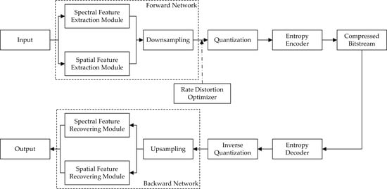
The network is an end-to-end framework based on a CNN and is composed of encoder and decoder. In the encoder, there are two parts for spectral feature extraction and spatial feature extraction, respectively. In the first part, continuous spectral feature extraction modules are adopted to extract spectral features independently. This part does not involve the fusion of spatial information. The second part is for spatial feature extraction, which contains several residual blocks. We use group convolution to separate each channel, so that only spatial features can be extracted without mixing the spectral information within them. Afterwards, all features are fused together and then downsampling is employed to reduce the size of the feature map. Additionally, to make the data more compact, a rate-distortion optimizer is used in the network. After obtaining the intermediate feature data, quantization and lossless entropy encoding are carried out to obtain the compressed binary bit stream. In the decoder, the bit stream first goes through entropy decoding and inverse quantization, and then upsampling helps to restore the image size. Finally, spectral and spatial features are acquired by corresponding deconvolution operations, and the joint feature is used to reconstruct the image. Experimental results demonstrate that our network surpasses JPEG2000 and 3D-SPIHT.

The remainder of this paper is organized as follows. Section 2 introduces our proposed network framework and principal analysis, Section 3 includes experimental parameter settings and the training process, and Section 4 presents the results and comparison with JPEG2000, 3D-SPIHT and the method mentioned in [20] at the same bit rate, which proves the wonderful performance of our network.

2. Proposed Method

In this section, we introduce the proposed multispectral image compression network framework in detail and describe the training flow diagram. We elaborate on several key operations, such as spectral feature extraction module, spatial feature extraction module, rate-distortion optimizer, etc.

2.1. Spectral Feature Extraction Module

2D convolution has been proven with great promise and successfully applied to lots of aspects of image vision and processing, such as target detection, image classification and image compression. However, as multispectral images are three-dimensional, which is more complex, and rich spectral information is even more important, the information loss problem will inevitably be encountered when 2D convolution is used to process multispectral images. Although there have been many precedents of applying deep learning to multispectral image compression, and it has achieved great performance and exceeded some traditional compression methods such as JPEG and JPEG2000, in the process of feature extraction, however, as the convolution kernel is two-dimensional, the spectral redundancy on the third dimension cannot be efficaciously removed, which inhibits the performance of the network.

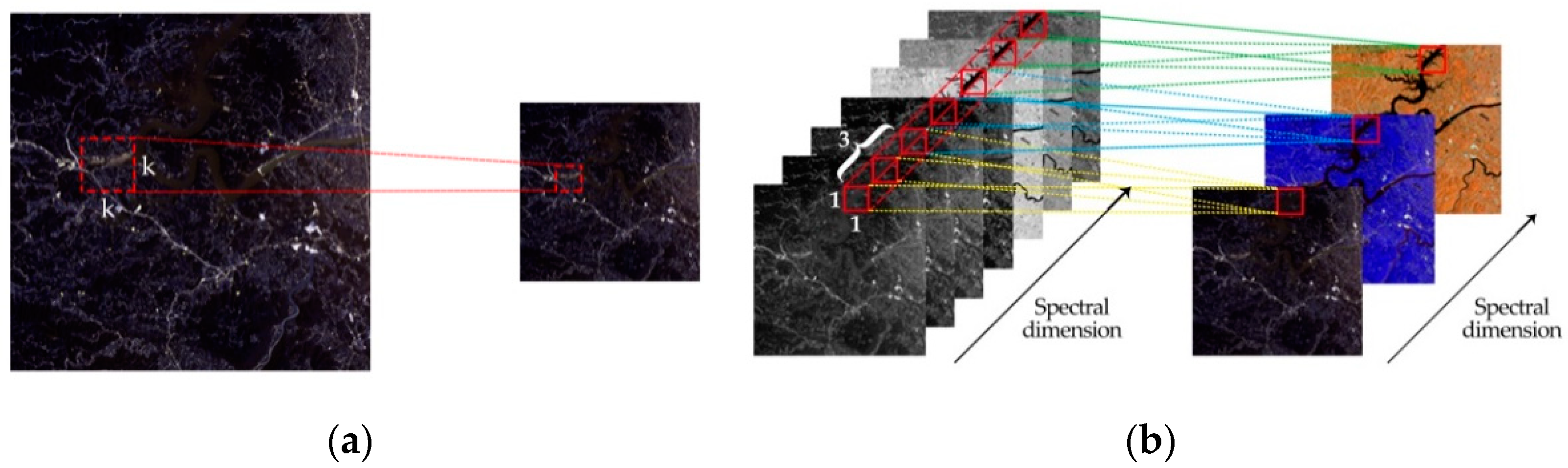
To deal with this problem, we have come up with the idea of extracting spectral or spatial features separately. Among this, the inspiration of extracting spectral features derives from [21]. Ref. [21] uses three-dimensional kernels for convolution operation, which can maintain the integrity of spectral features in multispectral image data. To avoid the data volume becoming too large, we use a $1\times 1\times n$ convolution kernel on the spectral dimension named as 1D spectral convolution to extract spectral features independently. Figure 1 shows the differences between 2D convolution and 1D spectral convolution.

As shown in Figure 1a, the image is convolved by 2D convolution, whose kernel is two-dimensional, generally followed by activation functions, such as rectified linear units (ReLU) [14], parametric rectified linear units (PReLU) [22], etc. This operation can be expressed as follows:

$$v_{ij}^{xy}=f\left({\displaystyle \sum _{m=1}^{M_{i-1}}{\displaystyle \sum _{p=0}^{P_i-1}{\displaystyle \sum _{q=0}^{Q_i-1}{w}_{ijm}^{pq}{v}_{(i-1)m}^{(x+p)(y+q)}+b_{ij}}}}\right),$$

(1)

where $i$ indicates the current layer, $j$ indicates the current feature map of this layer, $v_{ij}^{xy}$ is the output value at $\left(x,y\right)$ of the $j\text{-}\mathrm{th}$ feature map in the $i\text{-}\mathrm{th}$ layer, $f(\cdot )$ represents the activation function, $w_{ijm}^{pq}$ denotes the weight of the convolution kernel at position $\left(p,q\right)$ connected to the $m\text{-}\mathrm{th}$ feature map ($m$ indexes over the set of feature maps in the $\left(i-1\right)\text{-}\mathrm{th}$ layer connected to the current feature map), $b_{ij}$ is the bias of the $j\text{-}\mathrm{th}$ feature map in the $i\text{-}\mathrm{th}$ layer, $M_{i-1}$ is the number of feature maps in the $\left(i-1\right)\text{-}\mathrm{th}$ layer, $P_i$ and $Q_i$ are the height and width of the convolution kernel, respectively.

Similarly, considering the dimension of the spectrum, 1D spectral convolution operated on 3D images can be formulated as follows:

$$v_{ij}^{xyz}=f\left({\displaystyle \sum _{m=1}^{M_{i-1}}{\displaystyle \sum _{p=0}^{P_i-1}{\displaystyle \sum _{q=0}^{Q_i-1}{\displaystyle \sum _{r=0}^{R_i-1}{w}_{ijm}^{pqr}{v}_{(i-1)m}^{(x+p)(y+q)(z+r)}+b_{ij}}}}}\right),$$

(2)

where $R_i$ is the size of the convolution kernel in the spectral dimension, $v_{ij}^{xyz}$ is the output value at $\left(x,y,z\right)$ of the $j\text{-}\mathrm{th}$ feature map in the $i\text{-}\mathrm{th}$ layer, and $w_{ijm}^{pqr}$ is weight of the kernel at position $\left(p,q,r\right)$ connected to the $m\text{-}\mathrm{th}$ feature map. As the size of kernel is $1\times 1\times n$, by extension, $P_i$ and $Q_i$ are set to 1, Equation (2) can be written as:

$$v_{ij}^{xyz}=f\left({\displaystyle \sum _{m=1}^{M_{i-1}}{\displaystyle \sum _{r=0}^{R_i-1}{w}_{ijm}^{pqr}{v}_{(i-1)m}^{(x+p)(y+q)(z+r)}+b_{ij}}}\right),$$

(3)

In regard to the activation function, we adopt ReLU as our first choice, as the gradient is usually constant in back propagation when using ReLU, which alleviates the problem of gradient disappearance in deep network training and contributes to network convergence. Additionally, the computation cost is much less when using ReLU than other functions (e.g., sigmoid). In addition, ReLU can make the output of some neurons zero, which ensures the sparsity of the network so as to alleviate the overfitting problem. The ReLU function can be formulated as below:

$$f\left(x\right)=max\left(0,x\right).$$

(4)

In summary, when 2D convolution is operated on three-dimensional images, the output is always two-dimensional, which may cause a large amount of spectral information loss. Therefore, we adopt 1D spectral convolution to retain more feature data of the multispectral image.

2.2. Spatial Feature Extraction Module

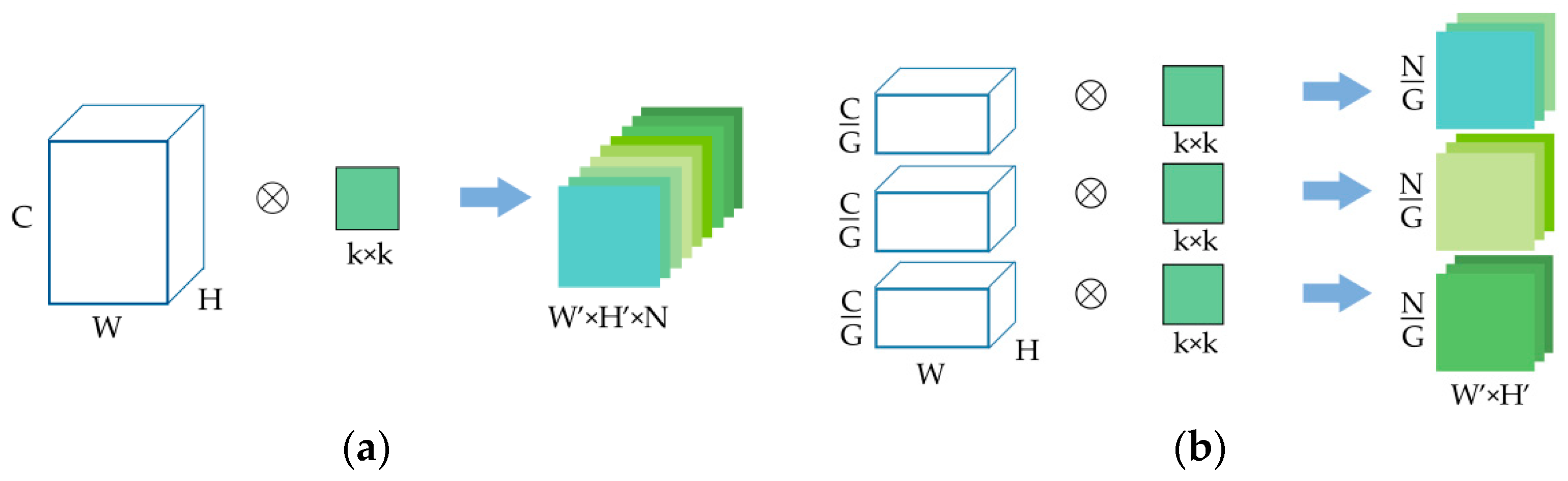
In order to ensure the spatial information does not mingle with the spectral features, we use group convolution instead of normal 2D convolution in spatial dimensions. Group convolution first appeared in AlexNet, in order to solve the problem of limited hardware resources at that time. Feature maps were distributed to several GPUs for simultaneous processing, and finally concatenated together. Figure 2 shows the differences between normal convolution and group convolution.

As shown in Figure 2a, the size of input data is $C\times H\times W$, representing the number of channels, width, and height of the feature map, respectively. The size of the convolution kernel is $k\times k$, and the number of the kernels is $N$. At this point, the size of the output feature map is $N\times H^{\prime }\times W^{\prime }$. The parameter number of N convolution kernels is:

$$params=N\times k\times k\times C.$$

(5)

In group convolution, just as its name implies, the input feature maps are divided into several groups, and then convolved separately. Assuming that the size of the input is still $C\times H\times W$ and the number of output feature maps is $N$. If the input is divided into $G$ groups, the number of input feature maps in each group is $C/G$, the number of output feature maps in each group is $N/G$, and the size of convolution kernel is $k\times k$, that is, the amount of convolution kernels remains unchanged and the number of kernels in each group is $N/G$. Since the feature maps are only convolved by the convolution kernels of the same group, the total number of parameters can be calculated as:

$$params=N\times k\times k\times \frac{C}{G}.$$

(6)

By comparing the two Equations (5) and (6), it can be easily known that group convolution can greatly reduce the number of parameters, precisely speaking, it can reduce them to $1/G$. Moreover, as group convolution can increase the diagonal correlation between filters according to [14], filter relationships become sparse after grouping.

Figure 3 shows the correlation matrix between filters of adjacent layers [23], highly correlated filters are brighter, while lower correlated filters are darker. The role of filter groups, namely group convolution, is to take advantage of the block-diagonal sparsity to learn information about the channel dimension. Low correlated filters do not need to be learned, that is to say, they do not need to be given parameters. What is more, as seen in Figure 3, the highly correlated filters can be trained in a more structured way when using group convolution. Therefore, with structured sparsity, group convolution can not only reduce the number of parameters, but also learn more accurately to make a more efficient network.

2.3. Framework of the Proposed Network

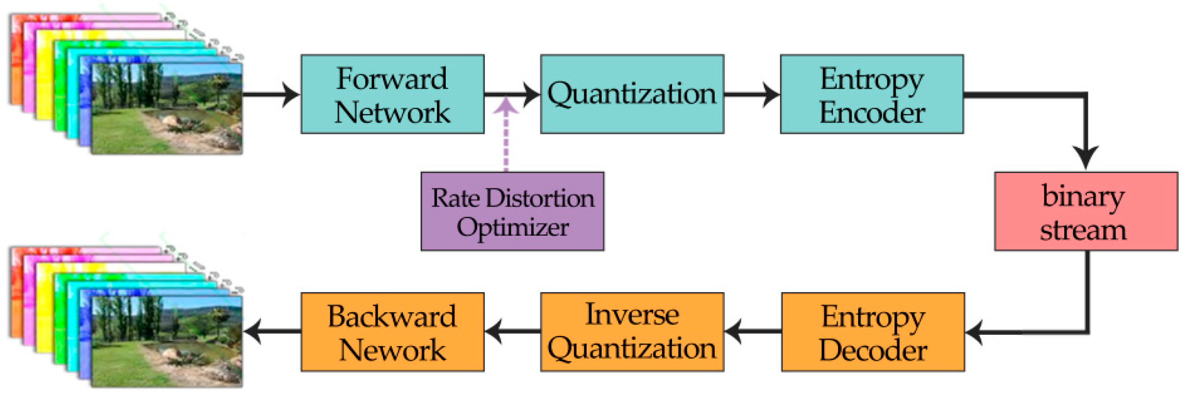
The whole framework of the proposed compression network is illustrated in Figure 4. The multispectral images are fed into the forward network first, after feature extraction, the data are then compressed and converted to bit stream successively through quantization and entropy encoder. The structure of the decoder is symmetrical with that of the encoder. As a result, for decoding, the bit stream goes through entropy decoding, inverse quantization, and the backward network, in turn, to restore the images. The detailed architecture of the forward and backward network will be demonstrated in Section 2.3.1.

2.3.1. The Forward Network and the Backward Network

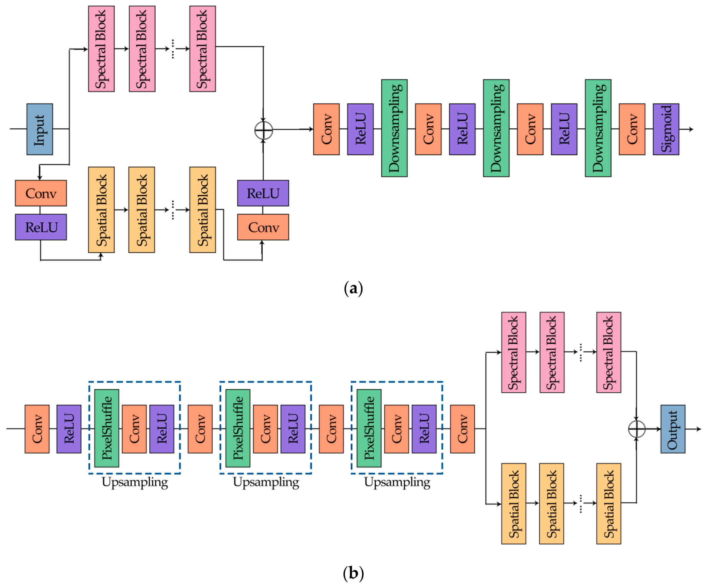
The architecture of the forward and backward network is shown in Figure 5, the spectral block and the spatial block are shown in Figure 6.

Figure 5 illustrates the detailed process of our network. First of all, the input multispectral images are simultaneously fed into the spectral feature extraction network and the spatial feature extraction network separately, which consist of corresponding function modules. In the spectral part, there are several spectral blocks (Figure 6a), which are based on residual block structure. We replace the convolution layers with 1D spectral convolution as adjusted to meet our expectations, and the size of the kernel is $1\times 1\times 3$. Likewise, the spatial part is composed by several spatial blocks with a similar structure, as shown in Figure 6b, and group convolution is used so that each channel will not interact with each other. To be specific, the GROUP is set to $7$ or $8$ as the input multispectral images are of seven or eight bands. Additionally, some convolution layers are added to enhance the ability of the learning features, whose kernel size is $3\times 3$. After extraction, two parts of the features are fused together, and then downsampling is carried out to reduce the size of the feature maps. At the end of the forward network, the sigmoid function plays a role of limiting the value of the intermediate output, in addition, similar to ReLU as well, it introduces nonlinear factors to make the network more expressive to the model.

Symmetric with the forward network, the backward network is formed with upsampling layers, some convolution layers, and the partitioned extraction part. In particular, upsampling is implemented with PixelShuffle [24], which can turn low resolution images into high resolution images using sub-pixel operation.

2.3.2. Quantization and Entropy Coding

After the forward network, the intermediate data are first quantized into a succession of discrete integers by the quantizer. Since the descent gradient is used in the backward propagation to update parameters when training the network, the gradient needs to be passed down. However, the rounding function is not differentiable [25], which will hinder the optimization of the network. Therefore, we relax the function, and it is calculated as:

$$X_Q=round\left[\left(2^Q-1\right)\times X_s\right],$$

(7)

where $Q$ is the quantization level, $X_s\in \left(0,1\right)$ is the intermediate datum after sigmoid activation, $round[\cdot ]$ is the rounding function, and $X_Q$ is the quantized data. The function rounds the data in the forward network and is skipped during backward propagation, to pass the gradient directly to the previous layer.

Then, we adopt ZPAQ as the lossless entropy coding standard and select “Method-6” as the compression pattern, in order to further process the quantized $X_Q$ and generate the binary bit stream. In the decoder, the bit stream goes through the entropy decoder and de-quantization, and the data $X_Q/\left(2^Q-1\right)$ are finally fed into the backward network to recover the image.

2.4. Rate-Distortion Optimizer

There are two criterions to evaluate a compression method, one is the bit rate, and the other is the quality of the recovered image. To enhance the performance of the network, it is vital to strike a balance between these two criterions. In consequence, rate-distortion optimization is introduced:

$$L=L_D+\lambda L_R,$$

(8)

where $L$ is the loss function that should be minimized during training, $L_D$ indicates the distortion loss, $L_R$ represents the rate loss, which can be controlled by the penalty $\lambda$. As we use MSE to measure the distortion loss of the recovered image, $L_D$ can be expressed as follows:

$$L_D=\frac{1}{N}\frac{1}{H\times W\times C}{\displaystyle \sum _{n=1,x,y,z}^N{\Vert I\left(x,y,z\right)-\tilde{I}\left(x,y,z\right)\Vert }^2},$$

(9)

where $N$ denotes the batch size, $I$ represents the original multispectral image and $\tilde{I}$ is the recovered image, $H$, $W$ and $C$ are, respectively, height, width, and spectral band number of the image.

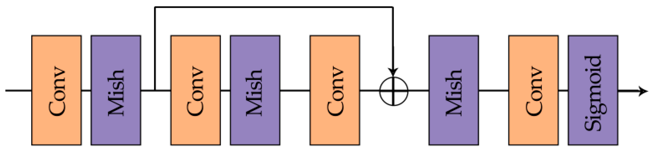
In order to estimate the rate loss, we adopt an Importance-Net to replace the entropy computation with a continuous approximation of the code length. The importance network is used to generate an importance map $P\left(X\right)$ learning from the input images [26]. The intention is to assign the bit rate according to the importance of the content of the image, more bits are assigned to complex regions, and fewer bits are assigned to smooth regions. The importance-net is simply composed of four layers, two $1\times 1$ convolution layers and a residual block that consists of two $3\times 3$ convolution layers, which is shown as Figure 7.

The activation function used in the importance-net is Mish [27], and it has been proven to be smoother than ReLU and achieve better results. Nonetheless, considering the time cost and limited hardware conditions due to the increased complexity of Mish, we only adopt Mish in the importance-net rather than the whole network. Mish can be formulated as:

$$Mish\left(x\right)=x\cdot \tanh \left(\ln \left(1+e^x\right)\right).$$

(10)

After sigmoid activation, the value range of the output is $\left[0,1\right]$. The importance map can be described as below:

$$\begin{array}{c}P\left(x,y\right)=\left[\widehat{X}\otimes w\right]\left(x,y\right)+b={\displaystyle \sum _{i=1}^k{\displaystyle \sum _{j=1}^k\left[{\widehat{X}}_n\left(s_{0}x+i,s_{0}y+j\right)w_n\left(i,j\right)\right]}}+b,\\ x\in \left\{0,1,\dots ,H\right\},y\in \left\{0,1,\dots ,W\right\},\end{array}$$

(11)

where $\widehat{X}$ represents the un-quantized output after the encoder, $w$ indicates the weight of the importance-net, $\left(x,y\right)$ is the spatial location of the pixel, and $b$, $k$ and $s_0$ are the bias, size of the kernel and stride, respectively. Unlike [26], we use the mean of $P\left(X\right)$ instead of the sum to define the rate loss:

$$P\left(X\right)={\displaystyle \sum _{N}P\left(x,y\right)},$$

(12)

$$L_R=\mathrm{avg}\left(P\left(X\right)\right),$$

(13)

where $N$ is the number of the intermediate channel.

3. Experimental Settings and Training

3.1. Datasets

The 7 band image datasets come from the Landsat-8 satellite. The training dataset contains about 80,000 images. The images we selected include various terrains under different seasons and different weather conditions, which enables the network to learn multiple features, preventing the network training from overfitting. We pick 17 representative images from 80,000 images as a test set and make sure that there are no identical images in the two data sets. The size of training images and test images are $128\times 128$ and $512\times 512$, respectively.

The 8 band image datasets come from the WorldView-3 satellite, which contains about 8700 images of size of $512\times 512$. Likewise, we ensure that the datasets include various terrains under different weather conditions to ensure the diversity of the feature. The test set has 14 images of size of $128\times 128$, and has no identical images with the training set.

3.2. Parameter Settings

We use the Adam optimizer to train the model and update the network. To accelerate the convergence of the network, the initial learning rate is set to 0.0001. Until the loss function drops to a certain degree, then set the learning rate to 0.00001 to seek for the optimal solution. The experimental settings of the training network are listed as

Table 1. Parameter settings.

Parameter	Value
Batch Size	16, 32
Learning Rate	1 × 10−4, 1 × 10−5
Inter-Channels	36, 48
$\lambda$	5 × 10−4, 1 × 10−3, 1 × 10−1, 5 × 10−1, 1, 5, 8

:

3.3. The Training Process

First of all, we initialize the weights of the network randomly, and utilize the Adam optimizer to train the network. In the first stage of training, MSE is introduced into the loss function. Since optimization is a process of restoring the image as close as possible to the original one, we can express it by the following formula:

$$\left({\tilde{\theta }}_1,{\tilde{\theta }}_2\right)=\arg \underset{{\theta }_1,{\theta }_2}{\min }{\Vert Re\left(En\left(Se\left({\theta }_1,x\right)+Sa\left({\theta }_2,x\right)\right)\right)-x\Vert }^2,$$

(14)

where $x$ is the original image, ${\theta }_1$ and ${\theta }_2$ are the parameters of the spectral feature extraction network and spatial feature extraction network, respectively. $Se(\cdot )$ represents the 1D spectral convolution network, $Sa(\cdot )$ is the spatial group convolution network, $En(\cdot )$ denotes quantization coding, and $Re(\cdot )$ denotes the whole decoding and recovering process. To make the loss function decline as soon as possible, ${\theta }_1$ and ${\theta }_2$ are disposed to update along with the gradient descent. By fixing ${\theta }_1$, we can obtain:

$${\tilde{\theta }}_2=\arg \underset{{\theta }_2}{\min }{\Vert Re\left(En\left(Se\left({\widehat{\theta }}_1,x\right)+Sa\left({\theta }_2,x\right)\right)\right)-x\Vert }^2,$$

(15)

and we can obtain ${\tilde{\theta }}_1$ by fixing ${\theta }_2$:

$${\tilde{\theta }}_1=\arg \underset{{\theta }_1}{\min }{\Vert Re\left(En\left(Se\left({\theta }_1,x\right)+Sa\left({\widehat{\theta }}_2,x\right)\right)\right)-x\Vert }^2.$$

(16)

During the backward propagation, the quantization needs to be skipped. Accordingly,

$$\left({\widehat{\theta }}_1,{\widehat{\theta }}_2\right)=\arg \underset{{\theta }_1,{\theta }_2}{\min }{\Vert Re\left(Se\left({\theta }_1,x\right)+Sa\left({\theta }_2,x\right)\right)-x\Vert }^2,$$

(17)

to simplify the representation of Equation (14), an auxiliary variable $x_m$ is introduced:

$$x_m\left({\theta }_1,{\theta }_2\right)=Se\left({\theta }_1,x\right)+Sa\left({\theta }_2,x\right),$$

(18)

hence, Equation (14) can be written as:

$$\left({\tilde{\theta }}_1,{\tilde{\theta }}_2\right)=\arg \underset{{\theta }_1,{\theta }_2}{\min }{\Vert Re\left(En\left(x_m\left({\theta }_1,{\theta }_2\right)\right)\right)-x\Vert }^2.$$

(19)

As the first stage of training optimization is completed, we then bring in the rate loss into the loss function. Combining Equations (13) and (19), the final optimization procedure can be formulated as:

$$\left({\tilde{\theta }}_1,{\tilde{\theta }}_2\right)=\arg \underset{{\theta }_1,{\theta }_2}{\min }\left\{{\Vert Re\left(En\left(x_m\left({\theta }_1,{\theta }_2\right)\right)\right)-x\Vert }^2+\mathrm{avg}\left[P\left({\theta }_1,{\theta }_2,x\right)\right]\right\}.$$

(20)

When the loss function no longer declines, the training reaches the optimal solution. Moreover, in the second stage of the training, a different compression rate can be easily obtained by changing the penalty $\lambda$. The value of $\lambda$ in our experiment is listed in Table 1.

4. Results and Discussion

In this section, we recorded the experimental results, including the performance comparison of our network with other traditional methods at the same bit rate, and the different bit rates have been obtained through adjusting the penalty $\lambda$. Meanwhile, to make the results more convincing, the compression method based on CNN using an optimized residual unit in [20] is also added for comparison. For presentation purposes, it is written as ResConv.

4.1. The Evaluation Criterion

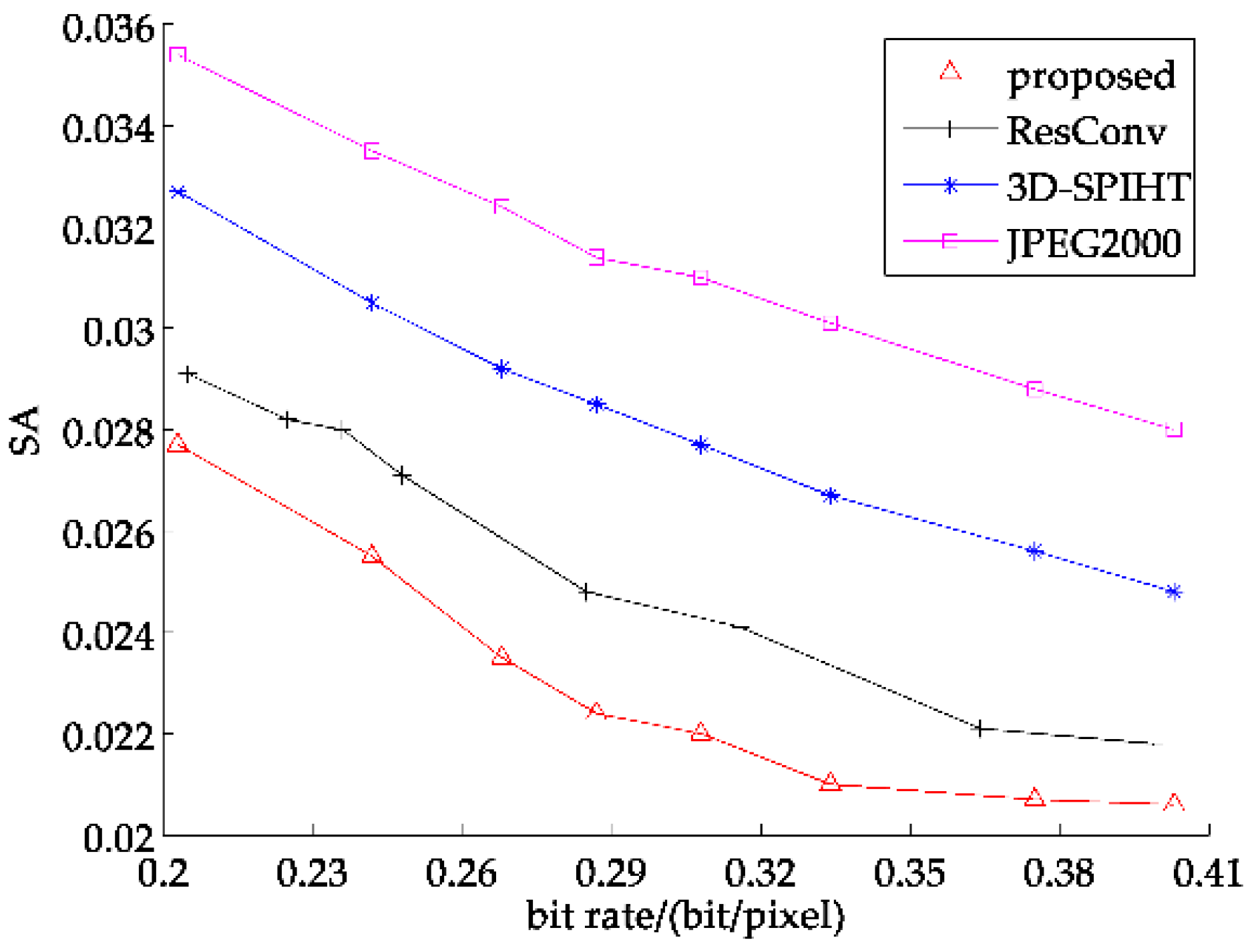
To evaluate the performance of the network comprehensively, apart from PSNR measuring the image recovery, we also utilize another metric known as spectral angle (SA) on the spectral dimension to verify the validity of the partitioned extraction method we proposed. SA indicates the angle between two spectra, which can be viewed as two vectors [28], and it can be used to measure the similarity between two spectral dimensions. The formula is written as follows:

$${\mathrm{SA}}_{I,\tilde{I}}={\cos }^{-1}\left(\frac{{\displaystyle \sum _{\lambda }\left(I\left(x,y,\lambda \right)\cdot \tilde{I}\left(x,y,\lambda \right)\right)}}{\sqrt{{\displaystyle \sum _{\lambda }{I}^2\left(x,y,\lambda \right)}{\displaystyle \sum _{\lambda }{\tilde{I}}^2\left(x,y,\lambda \right)}}}\right),$$

(21)

whose value ranges from −1 to 1. The closer the SA is to zero, the more similar the two vectors are.

4.2. Experimental Results

4.2.1. Spatial Information Recovery

Figure 8 shows the average PSNR of 7 band test sets. As seen from above, our proposed method is about 1 dB better than 3D-SPIHT and exceeds JPEG2000 by 3 dB. Comparing with ResConv, the partitioned extraction method still gains a little advantage of about 0.6 dB. Figure 9 states the detailed comparison of four selected test images, which can show the recovered result comparison of four methods. It is easy to tell that the partitioned extraction algorithm has an obvious superiority when the bit rate is ranging from 0.3–0.4.

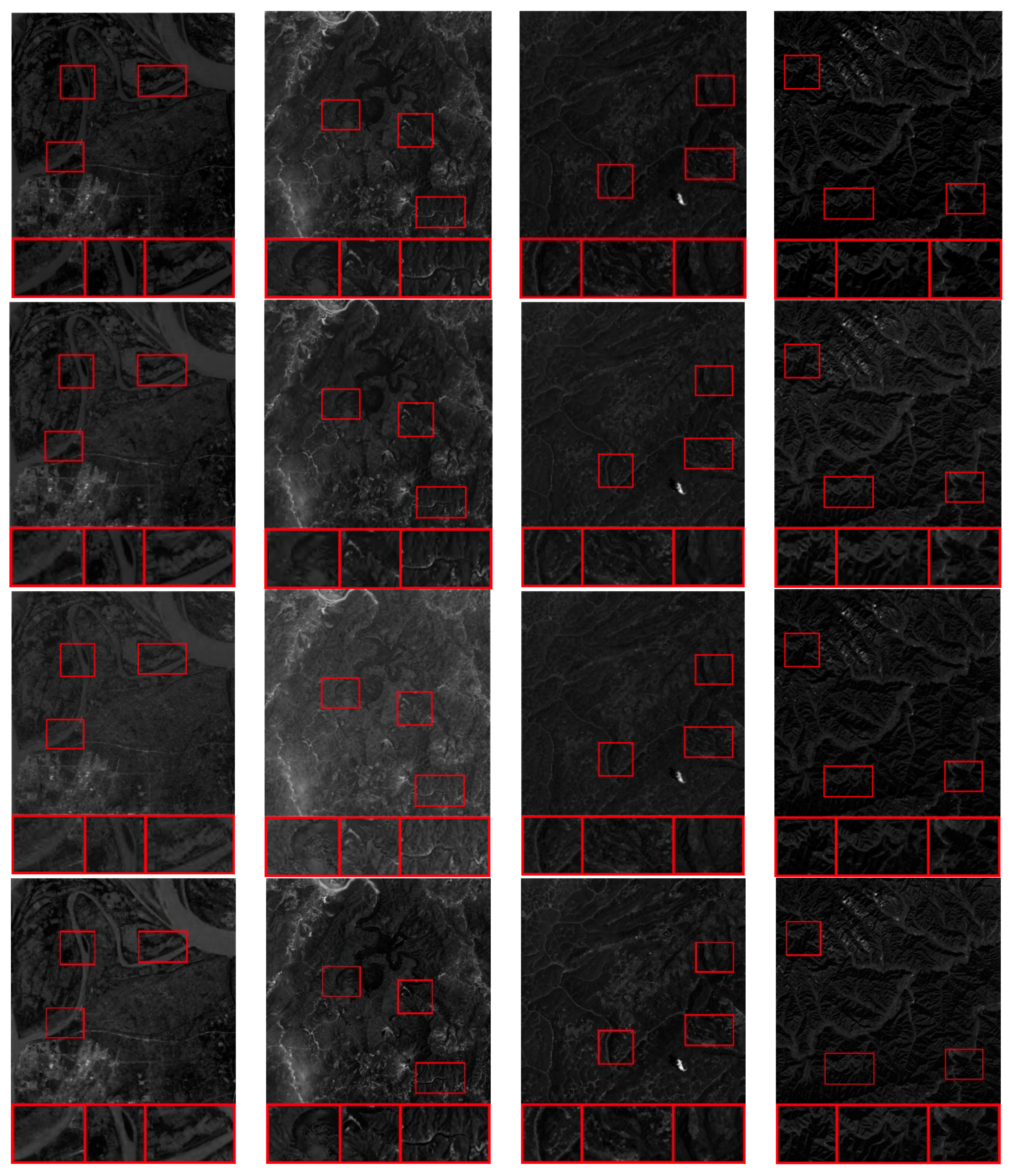
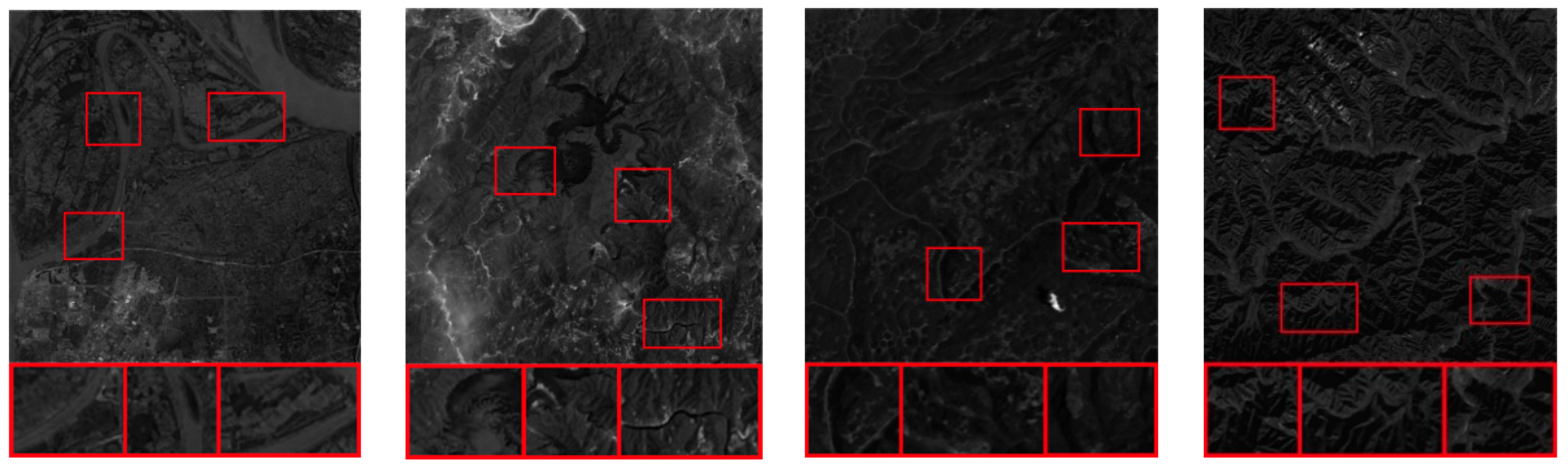
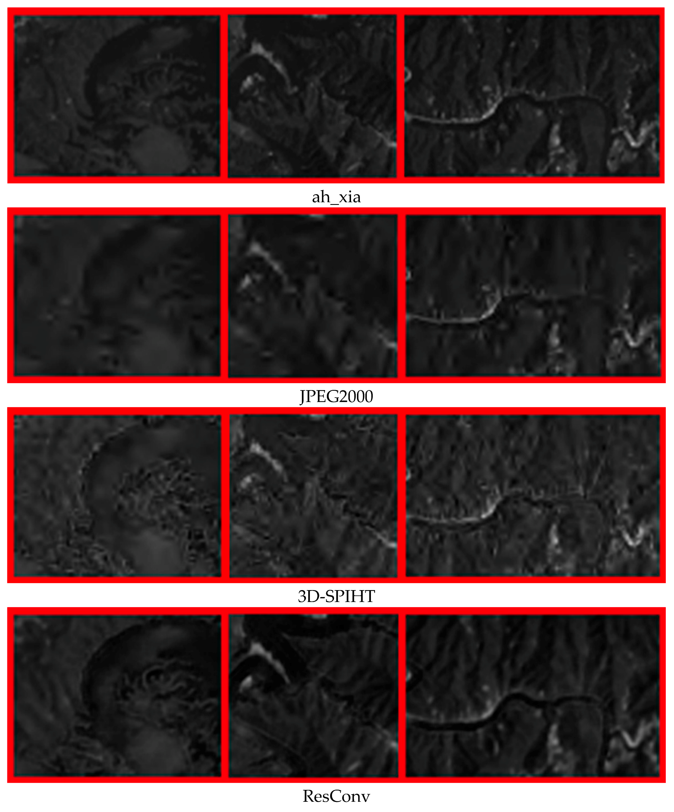
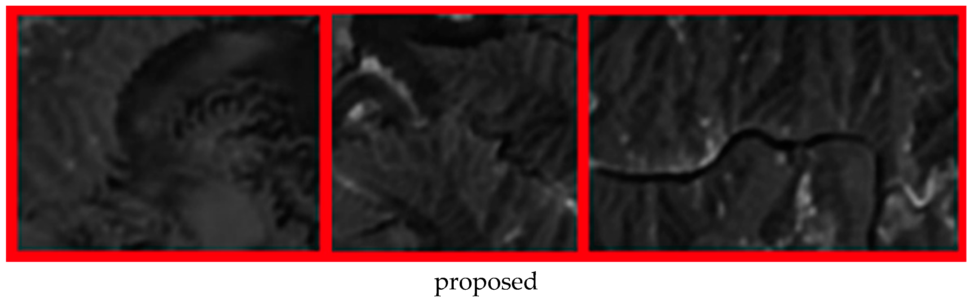
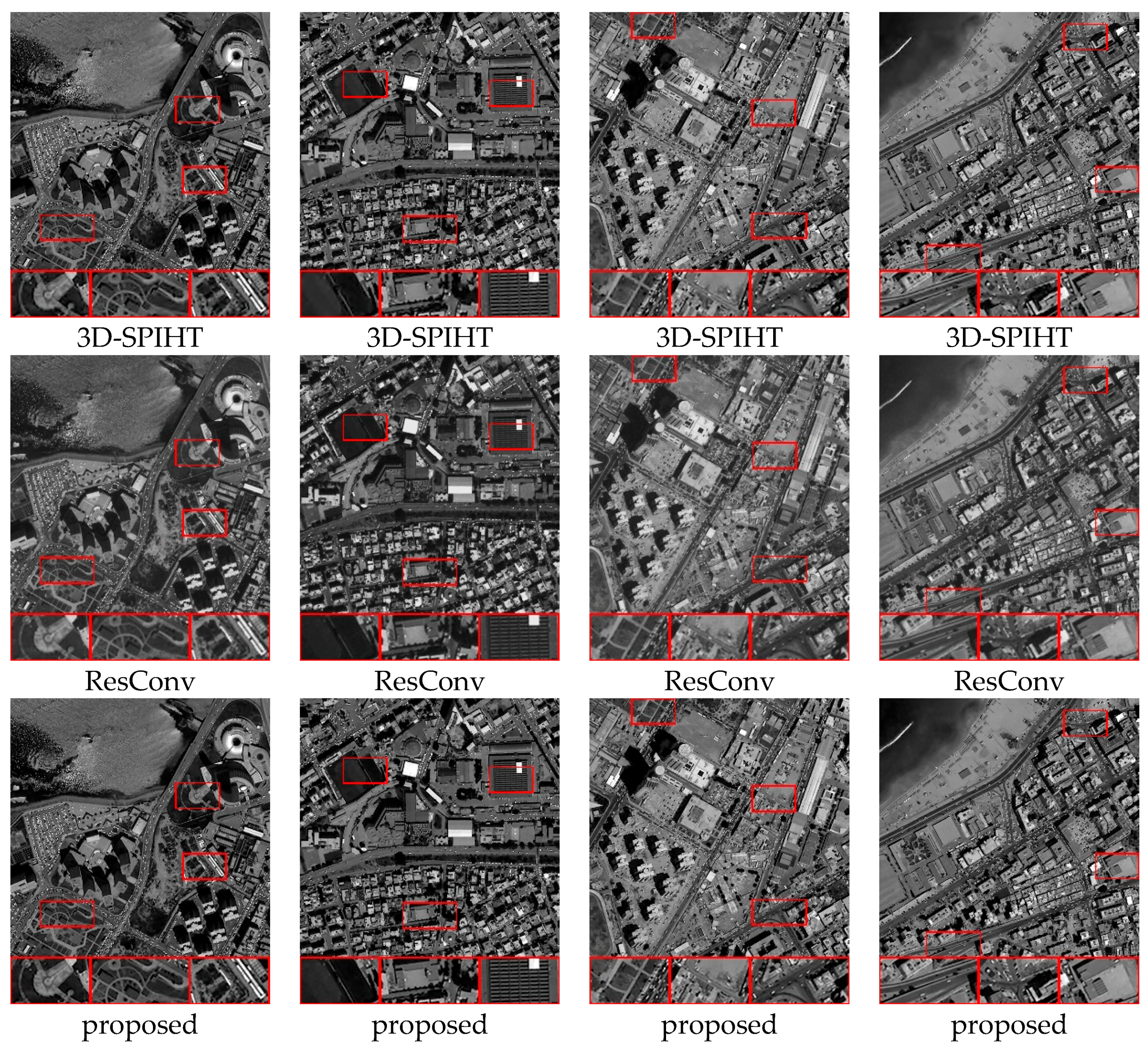
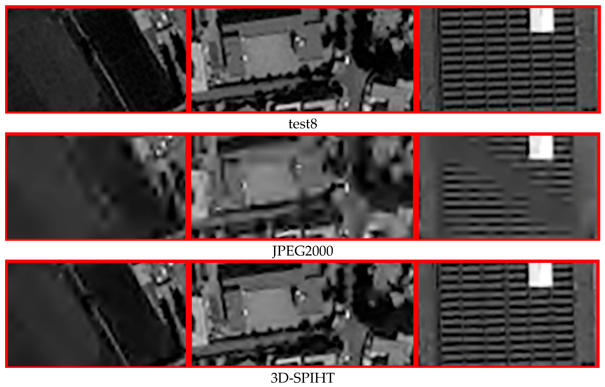
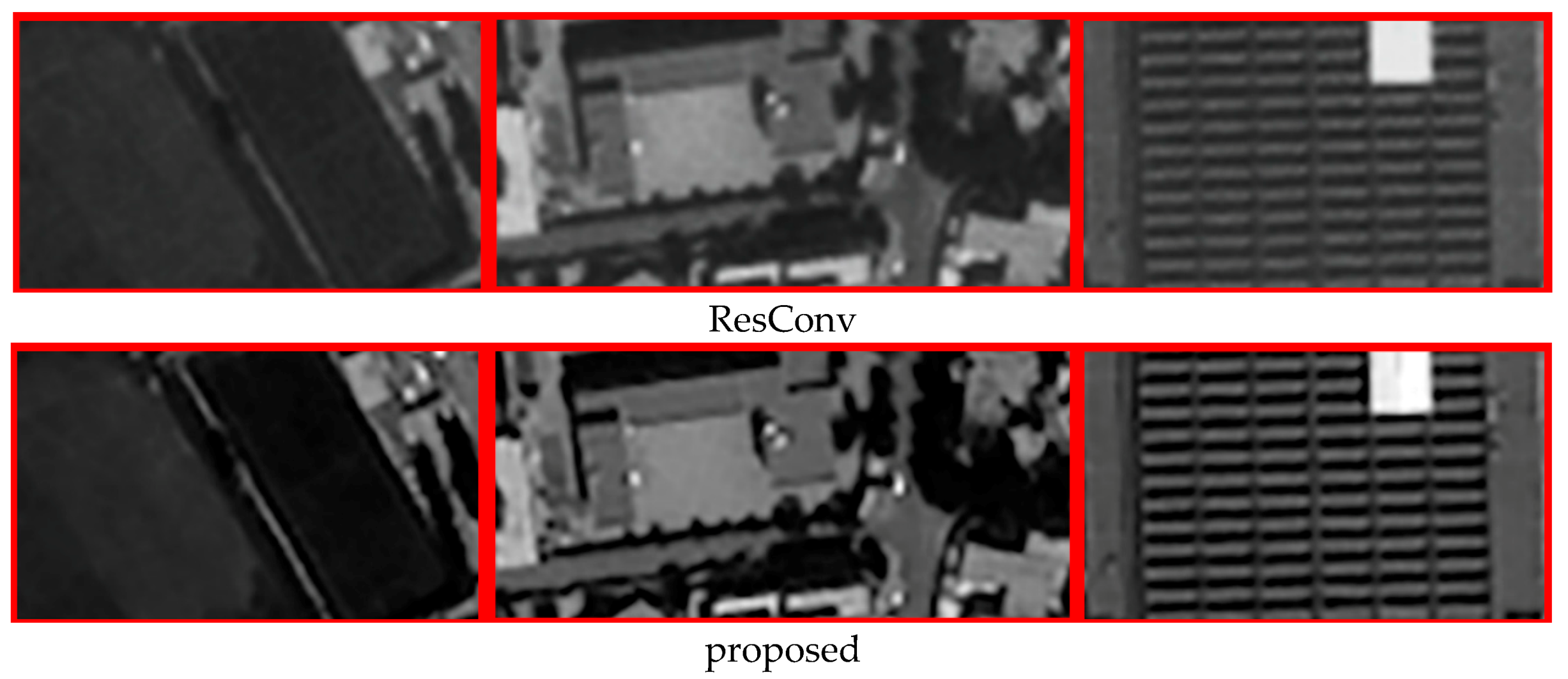
For illustrative purposes, Figure 10 shows the visual effects of four test images when the bit rate is around 0.4. To be specific, we display the grayscale image of the third band of the test image to show the differences more clearly. As can be seen from it, with the JPEG2000 and 3D-SPIHT algorithms, the recovered images have obvious block effects and the textures and margins are seriously blurred, whereas the proposed partitioned extraction algorithm performs well under the same bit rate, the same with ResConv, and these two methods preserve more details than any other methods. Figure 11 shows the partial enlarged view of ah_xia for a clearer demonstration. When the bit rate is around 0.4, ResConv and our proposed method both demonstrate impressive performance. However, according to Figure 8, ResConv starts to lose its edge as the bit rate drops to 0.3 or even lower and our method is then more stable.

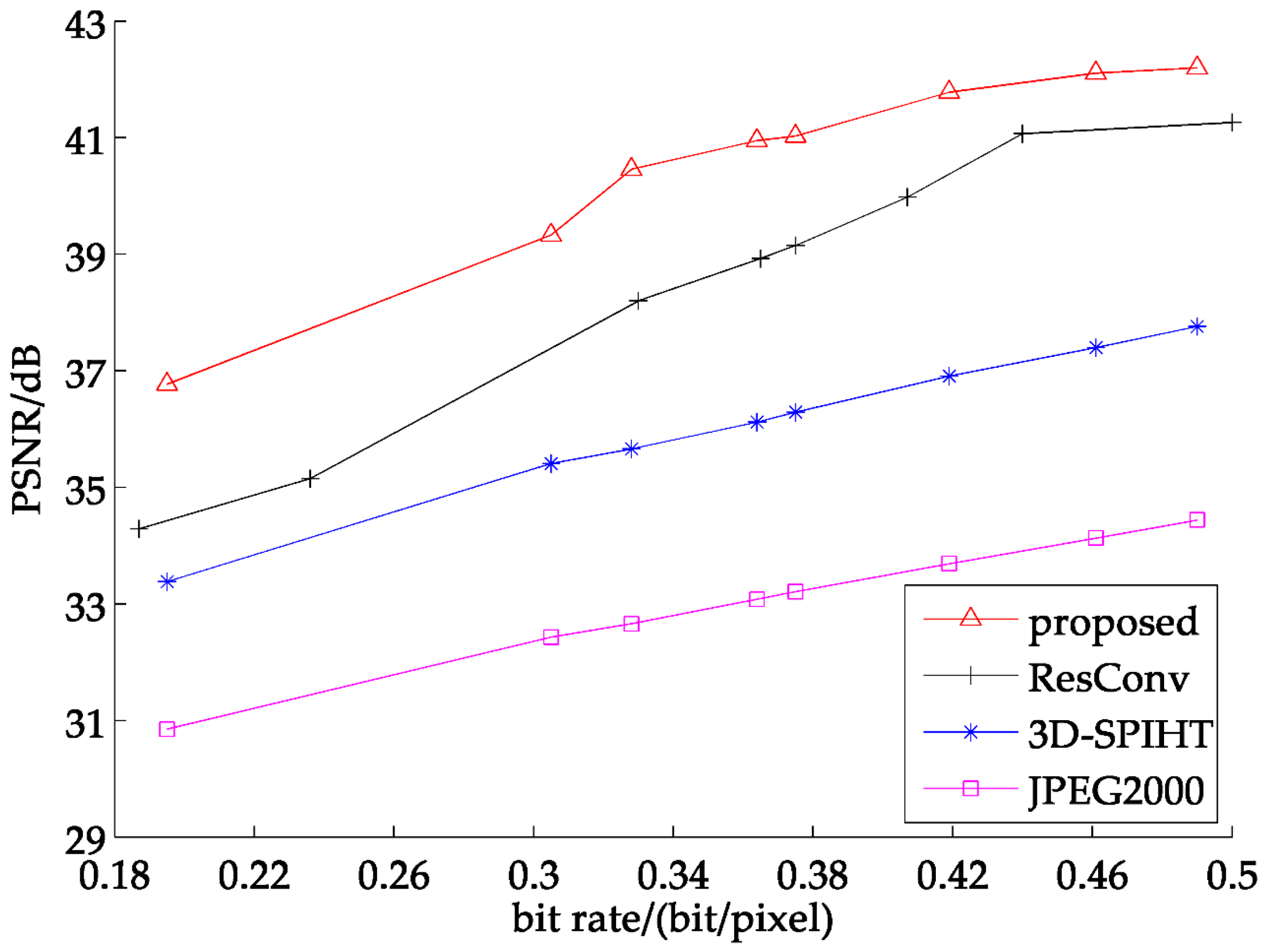
To further illustrate the advantage of our partitioned extraction method, we augment 8 band test sets into the experiment for better comparison. The average PSNR is shown in Figure 12. As seen from below, our method obtained a higher PSNR than JPEG2000 and 3D-SPIHT, approximately 8 dB and 4 dB, respectively. With regard to ResConv, the proposed method maintains the competitive edge and obtains about 2.5 dB higher than it on average.

Figure 13 represents the comparison of the PSNR of four test images from 8 band test sets at different bit rates. It can be observed that the advantage of the partitioned extraction method becomes quite prominent, compared with the result of the 7 band test images. Regarding ResConv, in spite of it surpassing JPEG2000 and 3D-SPIHT, its inferiority to our proposed method is more distinct compared with the results of the 7 band test sets. When it comes to processing multispectral images with more bands, or even hyperspectral images, some traditional compression methods will ineluctably be in a more inferior position, as they rarely take the abundant spectral correlation into account.

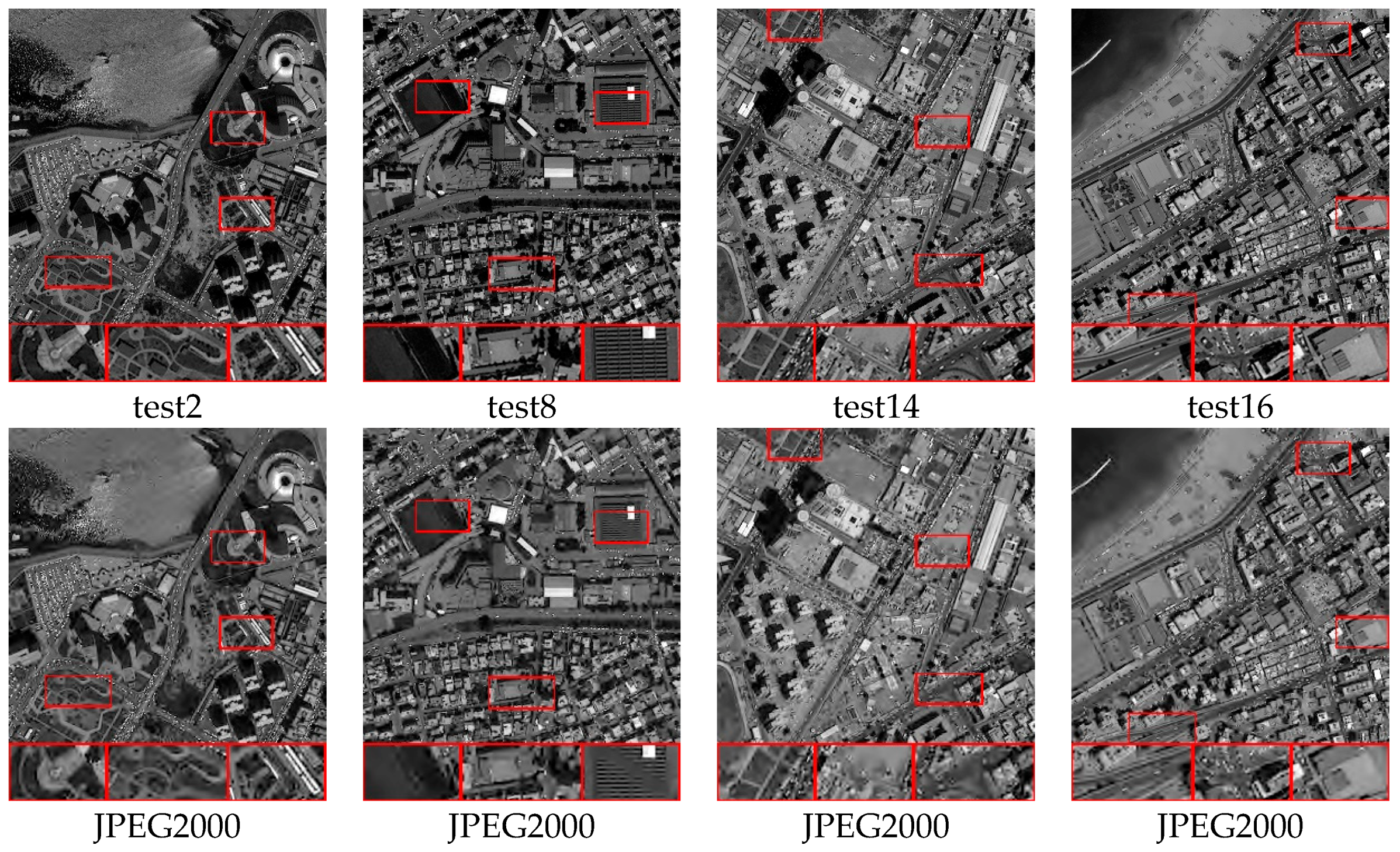
For visual comparison, as shown in Figure 14 and Figure 15, the JPEG2000 method inevitably generates serious block and ring effects, and detailed texture is ignored too. Furthermore, 3D-SPIHT is relatively better than JPEG2000; however, there are still a lot of blurred texture details in the recovered images. ResConv also obtains recovered images with blurred texture. On the contrary, the algorithm we proposed can retain the detailed texture and edge information of the images to a great extent.

All of the comparison results indicate that these traditional compression methods are not suitable for multispectral image compression, which may cause a lot spatial–spectral information loss. Some CNN-based algorithms may obtain a better result; however, as the bands increase, the inadequacy manifests as well. The partitioned extraction method of spatial–spectral features that we proposed has been proven effective on multispectral image compression, with its higher PSNR and much smoother visual effects.

4.2.2. Spectral Information Recovery

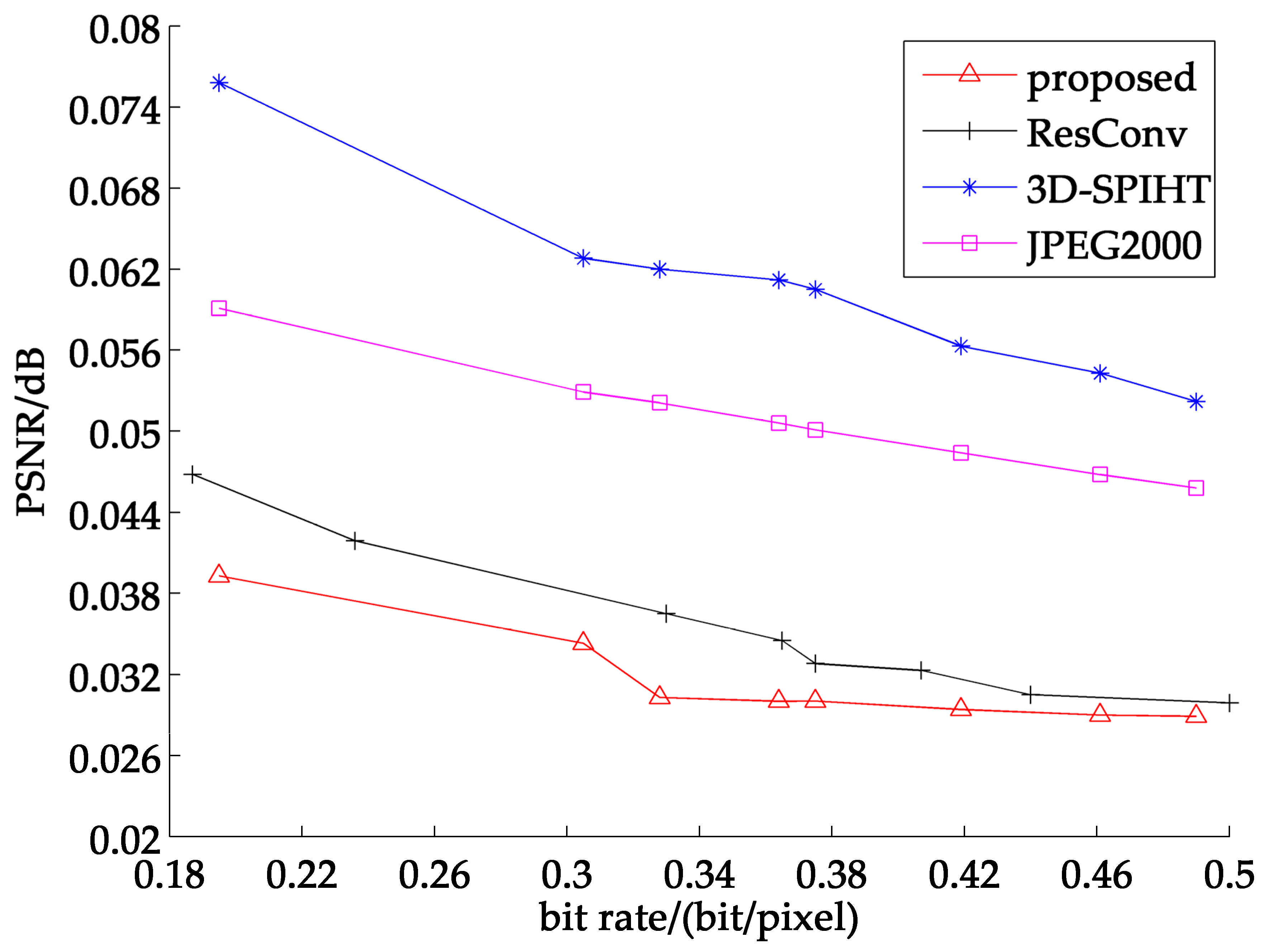
To adapt to our partitioned extraction network structure and verify the effectiveness of spectral information recovery as well, we adopt the SA as the second evaluation criterion. The average SA curves of 7 band and 8 band test sets are shown in Figure 16 and Figure 17, respectively. As seen below, we can find that the SA of the images reconstructed by the partitioned extraction algorithm is always smaller than that of JPEG2000, 3D-SPIHT and ResConv.

Table 2. SA of four 7 band test images (around a bit rate of 0.35).

Methods	ah_chun	ah_xia	hunan_chun	tj_dong
Proposed	0.0251	0.0192	0.0182	0.0180
ResConv	0.0265	0.0211	0.0206	0.0201
3D-SPIHT	0.0286	0.0301	0.0249	0.0253
JPEG2000	0.0324	0.0298	0.0255	0.0394

and

Table 3. SA of four 8 band test images (around a bit rate of 0.35).

Methods	Test2	Test8	Test14	Test16
Proposed	0.0348	0.0300	0.0289	0.0251
ResConv	0.0411	0.0377	0.0327	0.0312
3D-SPIHT	0.0576	0.0645	0.0571	0.0505
JPEG2000	0.0514	0.0517	0.0443	0.0397

list the detailed SA values of four representative test images of 7 band and 8 band, respectively. Supported by the chart and data below, it can be proven that the partitioned extraction algorithm obtains the smallest SA at all bit rates compared with the other three methods, and the smaller SA indicates that the images reconstructed by the proposed partitioned extraction method can obtain better spectral information recovery.

5. Conclusions

In this paper, a novel end-to-end framework with partitioned extraction of spatial–spectral features for multispectral image compression is proposed. The algorithm pays close attention to the abundant spectral features of the multispectral images and is committed to preserving the integrity of the spectral–spatial features. The spectral and spatial feature modules extract corresponding features separately, after which the features are fused together for further processing. Likewise, the spectral and spatial features are severally recovered when reconstructing the images, which can help obtain images with high quality. To testify the validity of the framework, experiments are implemented on both 7 band and 8 band test sets. The results show that the proposed algorithm surpasses JPEG2000, 3D-SPIHT and ResConv on PSNR, visual effects and SA as well. The results on the 8 band show that the proposed method has achieved a more obvious superiority, which may prove that spectral information plays an indispensable role in multispectral image processing.

References

- Li, Y.; Zhang, H.K.; Shen, Q. Spectral–Spatial Classification of Hyperspectral Imagery with 3D Convolutional Neural Network. Remote Sens. 2017, 9, 67. [Google Scholar] [CrossRef] [Green Version]
- Gelli, G.; Poggi, G. Compression of multispectral images by spectral classification and transform coding. IEEE Trans. Image Proc. 1999, 8, 476–489. [Google Scholar] [CrossRef] [PubMed]
- Zhou, Z.L. Research on Hyperspectral Image Compression Method. Master’s Thesis, Nanjing University of Science and Technology, Nanjing, China, 2008. [Google Scholar]
- Li, Y.S.; Wu, C.K.; Chen, J.; Xiang, L.B. Spectral satellite image compression based on wavelet transform. Acta Opt. Sin. 2001, 21, 691–695. [Google Scholar]
- Nian, Y.J.; Liu, Y.; Ye, Z. Pairwise KLT-based compression for multispectral images. Sens. Imaging 2016, 17, 1–15. [Google Scholar] [CrossRef]
- Slyz, M.; Zhang, L. A block-based inter-band lossless hyperspectral image compressor. In Proceedings of the IEEE Data Compression Conference, Snowbird, UT, USA, 29–31 March 2005; pp. 427–436. [Google Scholar] [CrossRef] [Green Version]
- Qian, S.E. Hyperspectral data compression using a fast vector quantization algorithm. IEEE Trans. Geosci. Remote Sens. 2004, 42, 1791–1798. [Google Scholar] [CrossRef]
- Hao, P.; Shi, Q. Reversible integer KLT for progressive-to-lossless compression of multiple component images. In Proceedings of the IEEE International Conference on Image Processing, Barcelona, Spain, 14–17 September 2003; p. I-633. [Google Scholar] [CrossRef] [Green Version]
- Abousleman, G.P.; Marcellin, M.W.; Hunt, B.R. Compression of hyperspectral imagery using the 3-D DCT and hybrid DPCM/DCT and entropy-constrained trellis coded quantization. In Proceedings of the Conference on Data Compression, Snowbird, UT, USA, 28–30 March 1995. [Google Scholar] [CrossRef]
- Sweldens, W. The Lifting Scheme: A Custom-Design Construction of Biorthogonal Wavelets. Appl. Comput. Harmon. Anal. 1996, 3, 186–200. [Google Scholar] [CrossRef] [Green Version]
- Tang, X.L.; Pearlman, W.A. Three-dimensional wavelet-based compression of hyperspectral images. In Hyperspectral Data Compression; Springer: Troy, NY, USA, 2006; pp. 273–308. ISBN 978-038-728-579-5. [Google Scholar]
- Dragotti, P.L.; Poggi, G.; Ragozini, A.R.P. Compression of multispectral images by three-dimensional SPIHT algorithm. IEEE Trans. Geosci. Remote Sens. 2000, 38, 416–428. [Google Scholar] [CrossRef]
- LeCun, Y.; Jackel, L.; Bottou, L.; Cortes, C.; Denker, J.S.; Drucker, H.; Guyon, I.; Müller, U.A.; Säckinger, E.; Simard, P.; et al. Learning algorithms for classification: A comparison on handwritten digit recognition. In Neural Networks: The Statistical Mechanics Perspective; World Scientific: Singapore, 1995; pp. 261–276. [Google Scholar] [CrossRef]
- Krizhevsky, A.; Sutskever, I.; Hinton, G.E. ImageNet classification with deep convolutional neural networks. In Proceedings of the 25th International Conference on Neural Information Processing Systems, Red Hook, NY, USA, 3–6 December 2012; pp. 1097–1105. [Google Scholar]
- Simonyan, K.; Zisserman, A. Very Deep Convolutional Networks for Large-Scale Image Recognition. Comput. Sci. 2014, arXiv:1409.1556v6. [Google Scholar]
- Szegedy, C.; Liu, W.; Jia, Y.Q.; Sermanet, P.; Reed, S.; Anguelov, D.; Erhan, D.; Vanhoucke, V.; Rabinovich, A. Going deeper with convolutions. In Proceedings of the 2015 IEEE Conference on Computer Vision and Pattern Recognition (CVPR), Boston, MA, USA, 7–12 June 2015; pp. 1–9. [Google Scholar] [CrossRef] [Green Version]
- He, K.; Zhang, X.; Ren, S.; Sun, J. Deep Residual Learning for Image Recognition. In Proceedings of the 2016 IEEE Conference on Computer Vision and Pattern Recognition (CVPR), Las Vegas, NV, USA, 27–30 June 2016; pp. 770–778. [Google Scholar] [CrossRef] [Green Version]
- Ballé, J.; Laparra, V.; Simoncelli, E. End-to-end Optimized Image Compression. In Proceedings of the 2017 International Conference on Learning Representations (ICLR), Toulon, France, 24–26 April 2017. [Google Scholar]
- Jiang, F.; Tao, W.; Liu, S.; Ren, J.; Guo, X.; Zhao, D. An End-to-End Compression Framework Based on Convolutional Neural Networks. IEEE Trans. Circuits Syst. Video Technol. 2018, 28, 3007–3018. [Google Scholar] [CrossRef] [Green Version]
- Kong, F.; Zhou, Y.; Shen, Q.; Wen, K. End-to-end Multispectral Image Compression Using Convolutional Neural Network. Chin. J. Lasers 2019, 46, 1009001-1. [Google Scholar] [CrossRef]
- Zhong, Z.; Li, J.; Luo, Z.; Chapman, M. Spectral–Spatial Residual Network for Hyperspectral Image Classification: A 3-D Deep Learning Framework. IEEE Trans. Geosci. Remote Sens. 2018, 56, 847–858. [Google Scholar] [CrossRef]
- He, K.; Zhang, X.; Ren, S.; Sun, J. Delving Deep into Rectifiers: Surpassing Human-Level Performance on ImageNet Classification. In Proceedings of the 2015 IEEE International Conference on Computer Vision (ICCV), Santiago, Chile, 7–13 December 2015; pp. 1026–1034. [Google Scholar] [CrossRef] [Green Version]
- A Tutorial on Filter Groups. Available online: https://blog.yani.io/filter-group-tutorial/ (accessed on 9 August 2020).
- Shi, W.Z.; Caballero, J.; Huszar, F.; Totz, J.; Aitken, A.P.; Bishop, R.; Rueckert, D.; Wang, Z. Real-time single image and video super-resolution using an efficient sub-pixel convolutional neural network. In Proceedings of the 2016 IEEE Conference on Computer Vision and Pattern Recognition (CVPR), Las Vegas, NV, USA, 27–30 June 2016; pp. 1874–1883. [Google Scholar]
- Toderici, G.; O’Malley, S.M.; Hwang, S.J.; Vincent, D.; Minnen, D.; Baluja, S.; Covell, M.; Sukthankar, R. Variable rate image compression with recurrent neural networks. arXiv 2015, arXiv:1511.06085v2. [Google Scholar]
- Li, M.; Zuo, W.; Gu, S.; Zhao, D.; Zhang, D. Learning Convolutional Networks for Content-Weighted Image Compression. In Proceedings of the 2018 IEEE/CVF Conference on Computer Vision and Pattern Recognition, Salt Lake City, UT, USA, 18–23 June 2018; pp. 3214–3223. [Google Scholar] [CrossRef] [Green Version]
- Misra, D. Mish: A Self Regularized Non-Monotonic Activation Function. arXiv 2019, arXiv:1908.08681. [Google Scholar]
- Christophe, E.; Leger, D.; Mailhes, C. Quality criteria benchmark for hyperspectral imagery. IEEE Trans. Geosci. Remote Sens. 2005, 43, 2103–2114. [Google Scholar] [CrossRef] [Green Version]
Figure 1.
(a) 2D convolution; (b) 1D spectral convolution.
Figure 2.
(a) Normal convolution; (b) group convolution.
Figure 3.
The correlation matrix between filters of adjacent layers: (a) 1 group; (b) 2 groups; (c) 4 groups; (d) 8 groups; (e) the correlation illustration.
Figure 4.
The flow diagram of the proposed network.
Figure 5.
(a) The forward network; (b) the backward network.
Figure 6.
(a) Spectral block; (b) spatial block.
Figure 7.
The Importance-Net.
Figure 8.
Average PSNR of 7 band test images at different bit rates.
Figure 9.
PSNR of recovered images: (a) ah_chun; (b) ah_xia.; (c) hunan_chun; (d) tj_dong.
Figure 10.
The visual comparison of the recovered images (each column represents the same image).
Figure 11.
Partial enlarged view of ah_xia.
Figure 12.
Average PSNR of 8 band test images at different bit rates.
Figure 13.
PSNR of recovered images: (a) test2; (b) test8; (c) test14; (d) test16.
Figure 14.
Figure 15.
Partial enlarged view of test8.
Figure 16.
Average spectral angle (SA) curve of 7 band test images.
Figure 17.
Average SA curve of 8 band test images.