
Elevation Spatial Variation Analysis and Compensation in GEO SAR Imaging


College of Electronic Science and Technology, National University of Defense Technology, No. 109 Deya Road, Changsha 410073, China
*
Author to whom correspondence should be addressed.
Remote Sens. 2021, 13(10), 1888; https://0-doi-org.brum.beds.ac.uk/10.3390/rs13101888
Submission received: 6 April 2021
/
Revised: 7 May 2021
/
Accepted: 8 May 2021
/
Published: 12 May 2021
(This article belongs to the Special Issue 2nd Edition Radar and Sonar Imaging and Processing)
Abstract
:Due to geosynchronous synthetic aperture radar’s (GEO SAR) high orbit and low relative speed, the integration time reaches up to hundreds of seconds for a fine resolution. The short revisit cycle is essential for remote sensing applications such as disaster monitoring and vegetation measurements. Three-dimensional (3D) scene imaging mode is crucial for long-term observation using GEO SAR. However, this mode will bring a new kind of space-variant error in elevation. In this paper, we focus on the analysis of the elevation space-variant error. First, the decorrelation problems caused by the spatial variation are presented. Second, by combining with the SAR imaging geometry, the elevation spatial variation is decomposed into two-dimensional (2D) space variation of range and azimuth. Third, an imaging algorithm is proposed to solve the 3D space variation and improve the focusing depth. Finally, simulations with dot-matrix targets and distributed targets are performed to validate the imaging method.
1. Introduction
Spaceborne synthetic aperture radar (SAR) is a radar system for ground observation with satellite as the carrier. Compared with low earth orbit SAR (LEO SAR), geosynchronous synthetic aperture radar (GEO SAR) has many advantages, such as high resolution, wide swath, being unaffected by national boundaries and meteorological conditions. Since the first civilian SAR satellite “Seasat” was launched by the National Aeronautics and Space Administration (NASA) in 1978 with a resolution of about 25 m, the current Terra-SAR-X system has a resolution of 0.15 m [1,2]. For the special requirement compared to LEO SAR, in 1978 the concept of GEO SAR was firstly proposed by K. Tomiyasu, and a preliminary and approximate analysis was performed assuming a particular orbit [3]. GEO SAR has bright application prospects in many significant research fields due to its ultra-long synthetic aperture time, wide swath, long dwell time and short revisit cycles, such as disaster monitoring and vegetation measurements [4,5]. The geosynchronous orbit can offer a much more flexible satellite than a low earth orbit, such as near-circle, near-ellipse, figure-8-like and some other complex tracks [6,7,8]. Recently, with the development of SAR systems, GEO SAR signal processing has been paid more attention, but higher resolution also means more complex challenges in SAR imaging.
As an import error source of spaceborne SAR, elevation spatial variation error has attracted the attention of many people. Due to the asymmetric satellite flight trajectory in the synthetic aperture time in the GEO SAR system, the range history changes of the targets with the same slant range in the beam center but different elevations are diverse [9]. At the same time, the Doppler chirp rate depends on the second derivative of the range history model [10]. Therefore, the azimuth matching filter is related to the terrain elevation [11] and only the azimuth matching filter of the reference point is matched, and other targets of different terrain in the scene will have distortion in the SAR imaging [8,12]. Given a symmetrical sensor flight path, a corresponding point can always be found in the 3D space of the irradiation scope, and the two have the same phase history in the received echo signal. However, for the asymmetric satellite flight path, no such corresponding point can be found, resulting in azimuth defocus. To sum up, for a target with a certain elevation in the GEO SAR system, due to the asymmetric trajectory of the satellite in the synthetic aperture time, the corresponding points that have exactly the same range history will not be found, which will cause the azimuth defocus of the imaging results [9].
However, most of the current studies only focus on the 2D space variation (range and azimuth), and the study on the elevation space variation is not comprehensive enough. For example, only the influence of elevation on focusing depth was studied even without quantification, and the factors such as wavelength and synthetic aperture time were not analyzed. For the compensation method is also through the sub-aperture method, processing in each sub-aperture segment [10,11], which leads to the existence of errors: focusing depth is poor (sub-aperture synthetic aperture time is short), stitching error and difficulty are large, a little splicing error will cause a large phase error. Sergi et al. proposed to compensate for the elevation error by dividing different azimuth sub-apertures and to invert the elevation for the Terra SAR-X Staring Spotlight (ST) mode, but the compensation effect becomes worse with the increase of the sub-aperture [13]. One straightforward approach is to perform a blockwise postfocusing, using an external DEM as suggested in [10], an approach based on existing topography-dependent motion compensation approaches [11,14,15]. On the other hand, because the orbit altitude of GEO SAR is about 36,000 km, a more accurate slant range model is necessary [16,17,18], and the second-order slant range model in geosynchronous orbit is no longer applicable. At present, some people have proposed the high-order Taylor expansion slant range model in the GEO SAR imaging algorithm [19,20,21], but it is only for the imaging of point targets and does not consider the elevation space variation. Or, the simple classical second-order slant range model is still adopted in some papers considering the elevation space variation [10,11,12], which will introduce a large phase error in GEO SAR. In recent studies, there has not been an analysis in GEO SAR that takes into account both the elevation space variation and the high-order slant range model.
Based on the previous research results, this paper comprehensively considers the use of high-order slant range model in the compensation of space-variant error caused by elevation. The coefficients of this model are related to range, azimuth and elevation. On account of Taylor expansion and series of inversion method [22], the high-order slant range model is taken into signal model, and the relationship of target elevation and location is considered, then the elevation spatial variation is decomposed to 2D range and azimuth spatial variation [23,24]. An improved Range-Doppler Azimuth Chirp Scaling (RD-ACS) algorithm is proposed by considering the high-order Taylor slant range model of spatial variation into the imaging processing. After the elevation decomposition, range spatially variant and azimuth time variant compensation are performed to achieve focusing processing. This allows imaging processing in the frequency domain to compensate for the 3D space variation involving the elevation space variation, eventually allowing to realize high-precision imaging.
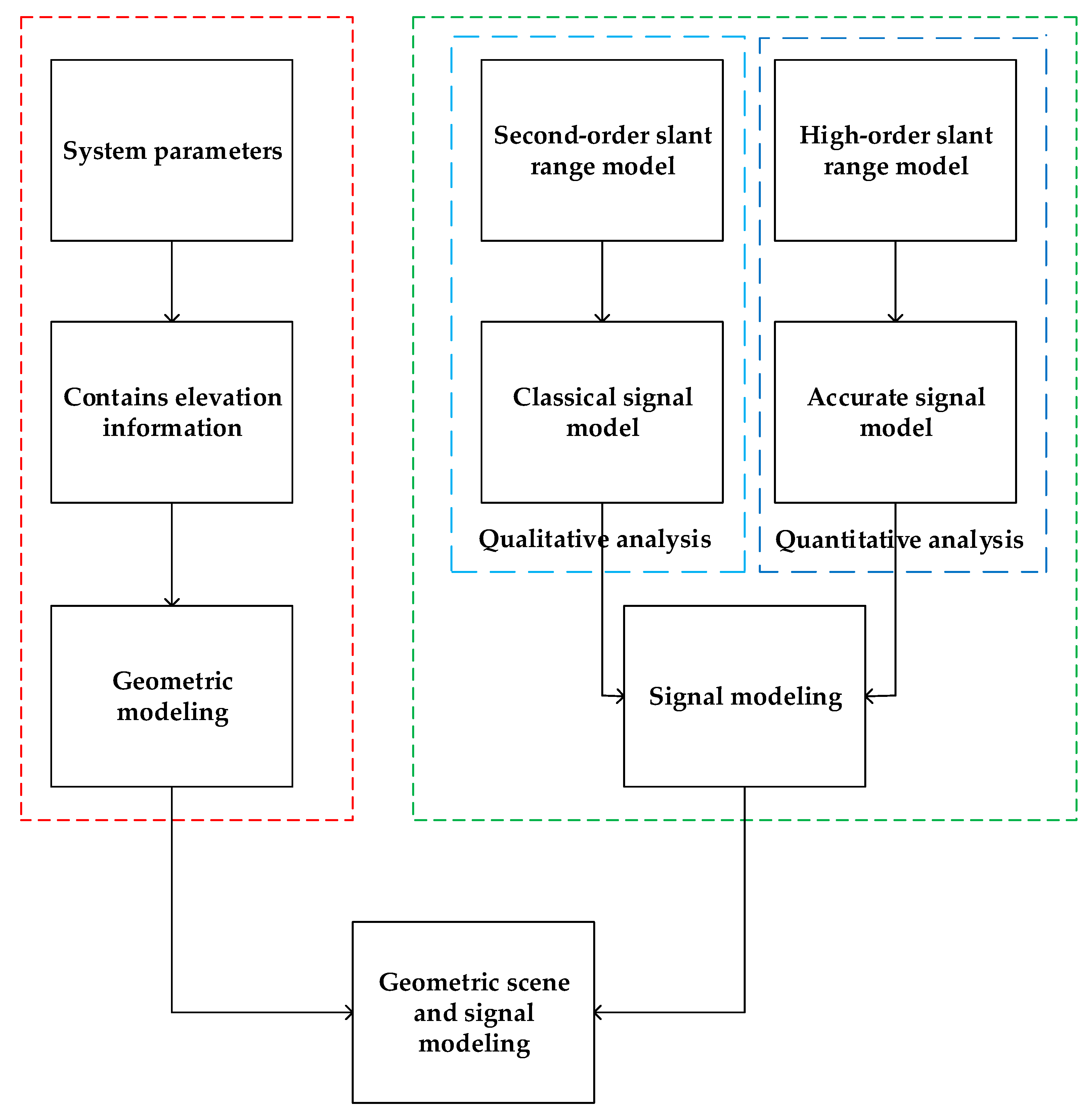
The structure of this paper is as follows: Section 2 establishes the 3D scene image geometric model. By considering the elevation into the echo signal model, the classical second-order slant range model and the high-order Taylor expansion slant range model are introduced into the echo signal, so that the influence of elevation can be determined quickly and accurately from both qualitative and quantitative aspects. Section 3 analyzes the influence of several factors such as elevation, different orbital positions, antenna sizes, wavebands and incident angles on the phase history of the target and the corresponding point, which provides reference for the practical application of GEO SAR. Section 4 discusses the imaging method of GEO SAR to compensate the elevation spatial variation error for the purpose of deep focus. Section 5 outlines the simulation experiments of dot-matrix targets and cone scenario to validate the proposed method. Section 6 and Section 7 summarize this paper, including a discussion on future research.
2. Geometric Scene and Signal Modeling with Elevation Information
We established a geometric imaging model that takes elevation information into consideration. Then, from the original echo signal, the effect of elevation information in echo was analyzed. The echo signal is expressed as:
where is any constant, is range time (fast time), is azimuth time (slow time), is center deviation time, is range envelope, is azimuth envelope, is radar center frequency, is chirp rate, is instantaneous slant range, and is the speed of light.
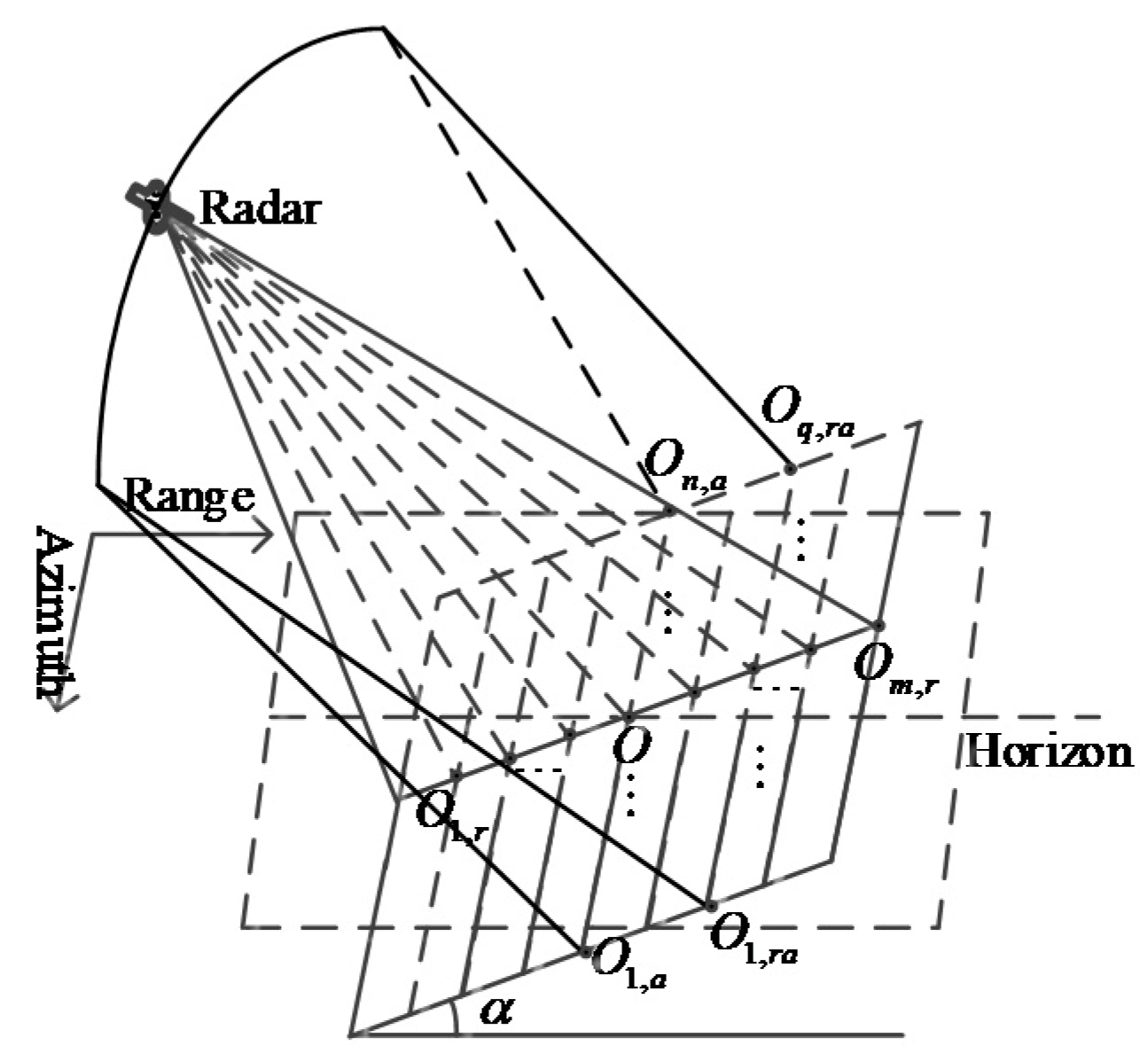
The 2D time-domain expression of echo signal is shown in Equation (1). The elevation information mainly affects the instantaneous slant range, which plays a crucial role in the SAR imaging algorithm. In the imaging processing of the GEO SAR system, since the orbit of the satellite is elliptical during synthetic aperture time, the classical second-order slant range model is no longer applicable, and an accurate slant range model must be adopted, which means that the expression will be more complicated. In order to analyze the effect of elevation on echo and subsequent imaging processing, we discuss it from both qualitative and quantitative perspectives. From the qualitative analysis level, the classical SAR imaging analysis process of second-order slant range is still adopted, but the elevation is taken into account on the original basis, so that the influence of elevation can be quickly analyzed. Then, an accurate high-order slant range expansion model was used to bring it into the echo to get the 2D spectrum of the signal. The phase was decomposed to analyze the influence of elevation on each decomposed phase, which provides theoretical support for the compensation of spatial variation in the imaging in the Section 4. The influence of elevation was quantitatively analyzed, and the correctness of the qualitative analysis was verified. The illustration of the GEO SAR geometric model and signal model is shown in Figure 1.
2.1. Signal Model Using the Second-Order Slant Range
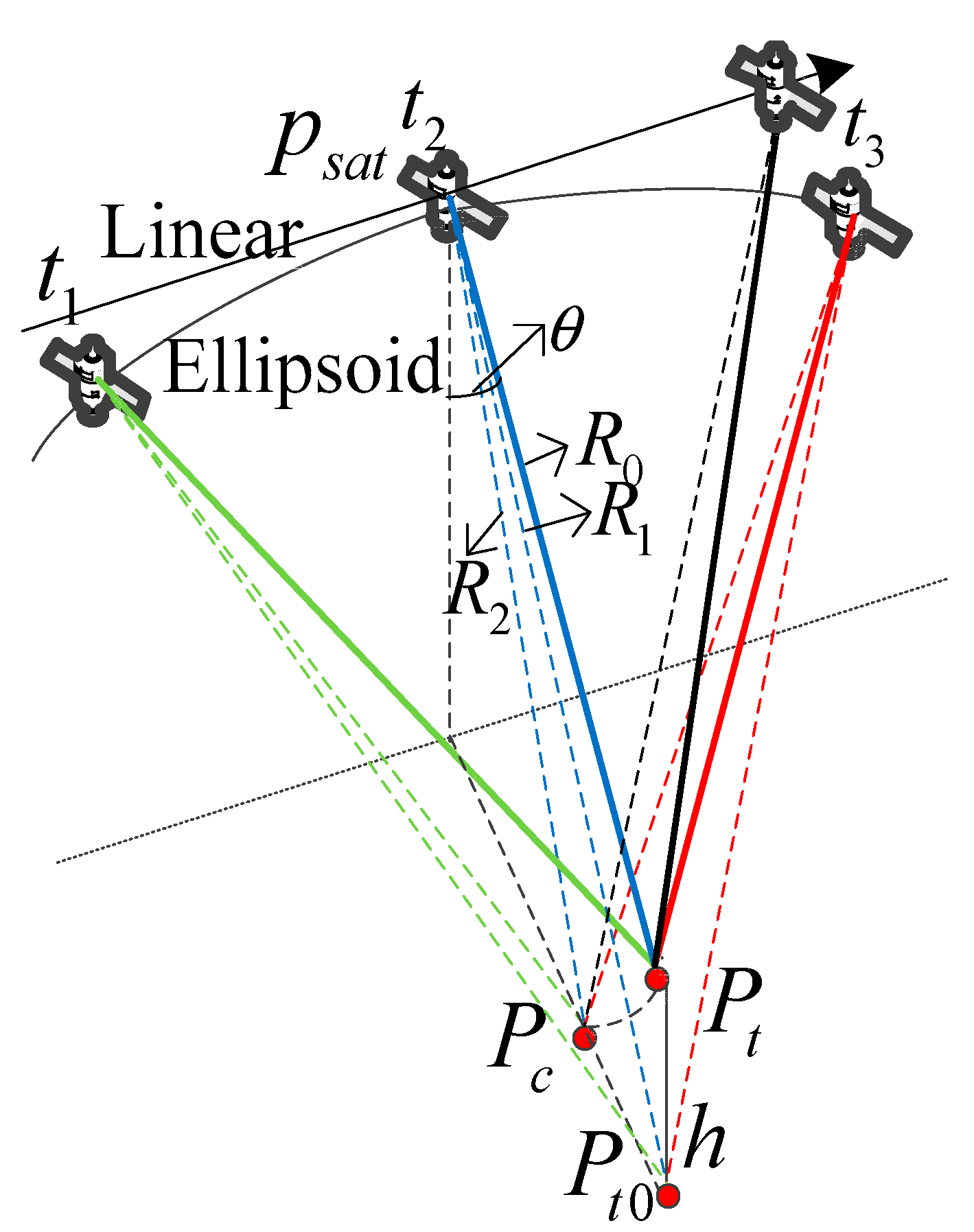
We firstly established a classical SAR imaging geometric model and the elevation information of the target was taken into account, as shown in Figure 2. The target elevation is , the look-down angle is , and the shortest slant range of the zero elevation target and the target is and respectively.
After adding elevation information, it can be known obviously that the closest slant range of the target decreases with the increase of elevation, while the effective velocity increases linearly with the increase of elevation [25].
From the perspective of signal model, the influence of elevation on imaging is analyzed by taking range-Doppler (RD) algorithm as an example. The echo after orthogonal demodulation is shown in Equation (1), and the signal after range pulse compression is:
where and represent the range history of and . It can be seen that range migration occurs in the range-direction envelope compared with the zero elevation after range compression. Similarly, the range equation is approximated to a parabola by referring to the classical SAR processing. Then the range compression signal can be expressed as:
where represents the effective velocity of . The azimuth chirp rate is and the chirp rate error increases as target elevation increases. Resulting in the imaging results azimuth defocuses, and the defocus becomes more serious with the increase of elevation. Then by using the principle of stationary phase (POSP), the time-frequency relation in the azimuth direction can be obtained as . The range migration in the range Doppler domain can be obtained, that is . It can be seen that the range migration error gradually increases with the increase of the target elevation.
Then the difference of the range migration compensation phase between the target and the zero elevation reference point is:
It can be seen that this phase term is very small; it is proportional to the fast time frequency and proportional to the square of the azimuth time frequency. After the range migration correction is realized through interpolation, the matching filter of the zero elevation target is used to focus the azimuth of the data in the range-Doppler domain, and the signal is:
As can be seen from the above equations, the second exponential phase of the focused signal is the secondary phase of , which will cause defocus in the azimuth direction, and the azimuth defocus will become more serious as increases. By comparing Equations (4) and (5), it can be seen that, compared with the range migration phase error, the phase term of azimuth compression is larger, which will cause serious azimuth defocus.
2.2. Signal Model Using the High-Order Slant Range
The synthetic aperture time of the GEO SAR system can reach hundreds of seconds, and the satellite trajectory is elliptical, as shown in Figure 2. represents the corresponding point of the target . The corresponding point is located on the ellipsoid surface, the distance between the target and the corresponding point at zero moment is equal to the satellite, and the position vector of the corresponding point to the satellite at zero moment is orthogonal to the satellite velocity vector. The corresponding point position coordinates can be solved through the above three conditions. At the same time, the slant range history of the target is relatively complex and requires a high-order slant range model with high precision. In this paper, the fifth-order Taylor expansion slant range model is adopted.
After the orthogonal demodulation of echo signal, the signal form is still as shown in Equation (1), but the slant range model is represented by the Taylor expansion high-order model, that is:
The high-order model of Taylor expansion is obtained by the azimuth time Taylor expansion of the numerical calculation model. For the solution of each order coefficient in the Taylor expansion model, the real slant range history can be directly fitted, and the fitting parameters obtained are the coefficients of each order. The fitting is related to the elevation of the target, and the coordinate solution of the corresponding point is also related to the elevation, so it can be clearly seen that the elevation has an impact on the slant range history. The stationary phase solution is obtained by series inversion [22]. The expression of stationary point can be found in Appendix A.
Then by put the stationary point into the Taylor expansion model, the final expression in the 2D frequency domain can be derived, namely:
where and represent the range and azimuth envelope in the frequency domain, respectively. The phase expression is further decomposed:
where is the range compression phase, is the azimuth compression phase, is the range migration phase, and the residual phase is . These expressions can be referred to Appendix B.
Further, the range migration expression is as follows:
And the effective velocity in the high-order Taylor expansion model should be calculated according to the following formula [26]:
For the fifth-order slant range model shown in Equation (6), the elevation of the target will affect and the coefficients of each order. In order to intuitively and quantitatively analyze the influence of the elevation, several groups of point targets with different elevations are set, and the target elevations are 200 m, 400 m, 600 m, 800 m, and 1000 m in turn. It can be clearly seen that the elevation information has no effect on the range compression phase. The influence of the elevation on the other decomposition phases is mainly analyzed below.
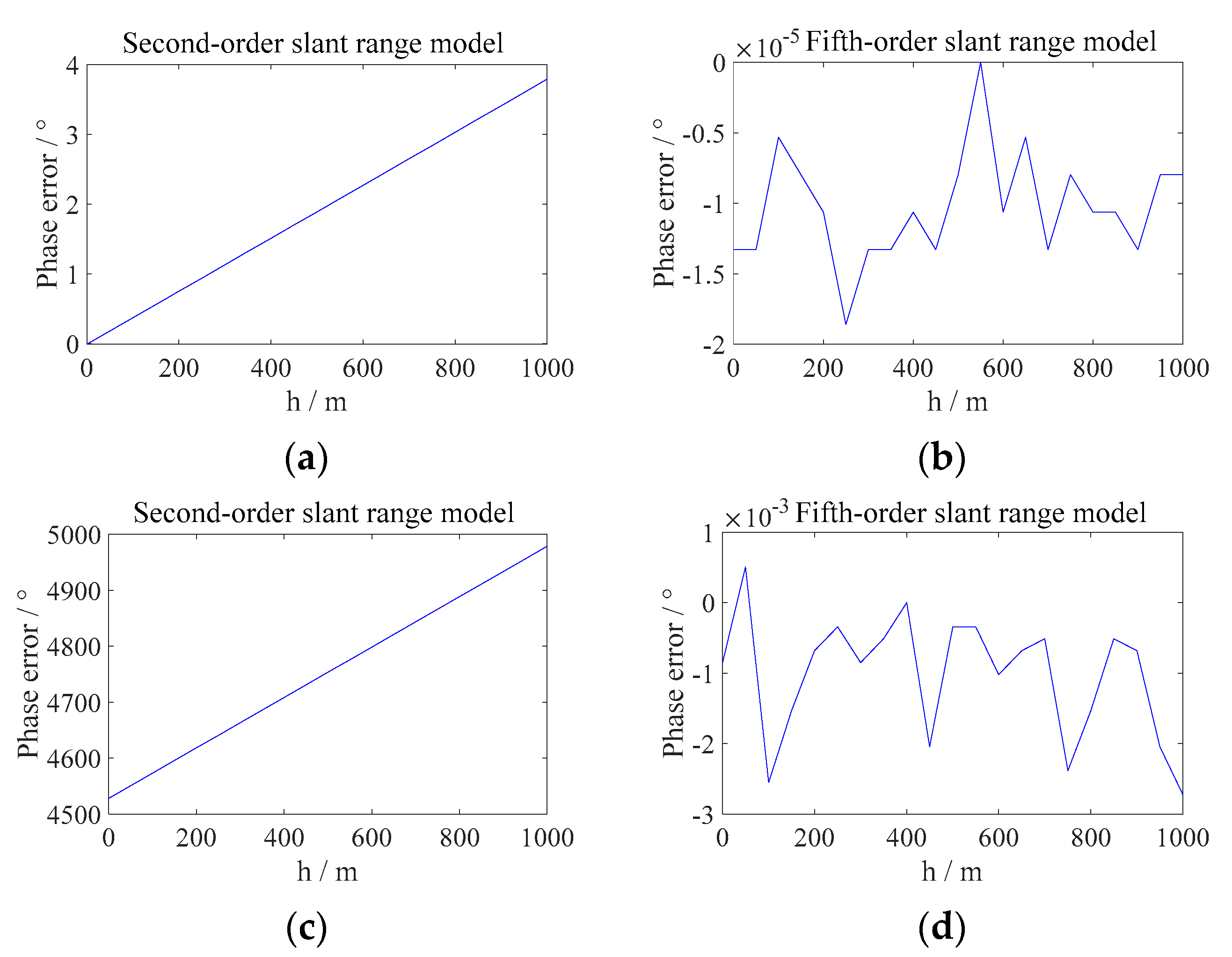
Firstly, the phase error variation with elevation is analyzed when the classical second-order slant range model and the fifth-order Taylor expansion slant range model are used as the target’s true slant range history in the LEO SAR and GEO SAR systems. The result is shown in Figure 3.
It can be seen that in the GEO SAR system, the phase error introduced by the second-order slant range model increases linearly with the elevation, while the error introduced by the fifth-order slant range model is negligible. However, the error caused by the second-order slant range model is still negligible in the LEO system.
The phase error variation of each decomposition phase with elevation is analyzed below. In the geometric model shown in Figure 2, the phase difference between target and target was selected as the research object in order to obtain the influence of elevation on each decomposition phase of the echo signal and correspond to the qualitative analysis in Section 2.1. However, in the SAR imaging processing, targets within the irradiation range are projected to the slant range of the antenna upward. In fact, the phase error introduced by the elevation is the phase difference between the target and its corresponding point . Therefore, this paper also analyzes the phase error introduced by the target elevation information in the focusing process of SAR image, and it analyzes it from each decomposed phase.
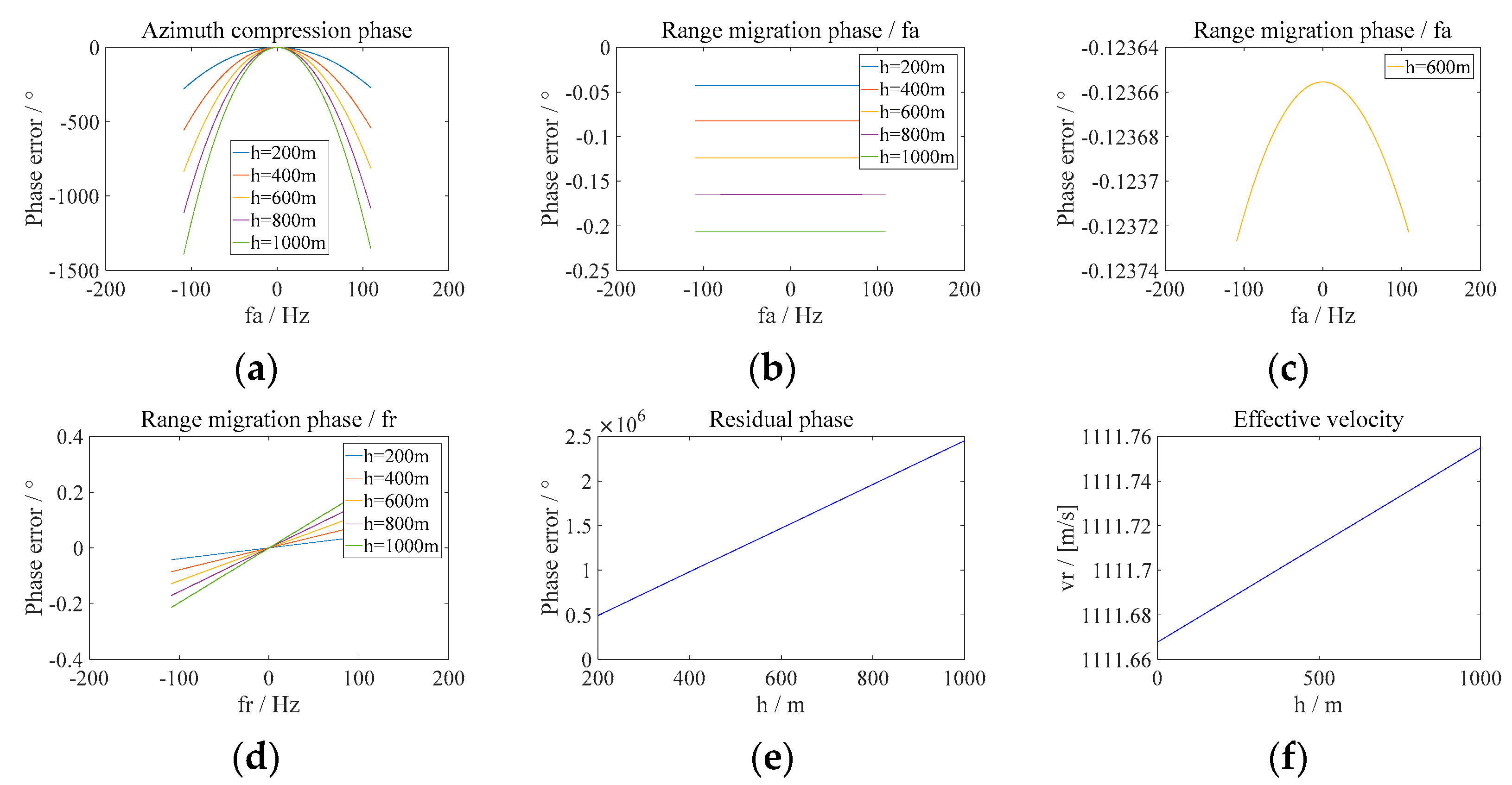
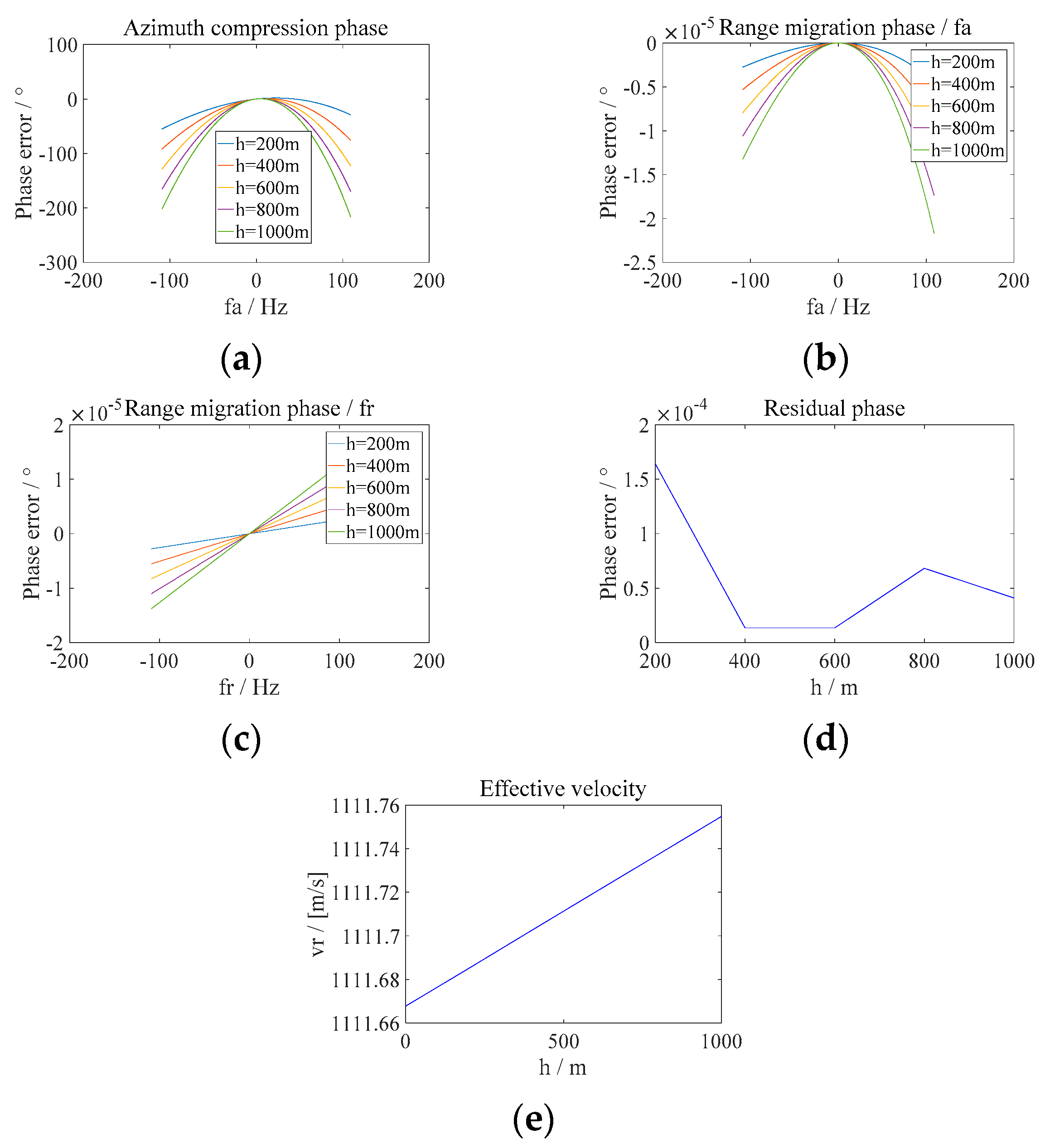
In order to correspond to qualitative analysis, the following results show several groups of 2D spectral decomposition phase difference of the echo between different elevation targets and zero elevation target: azimuth compression phase, range migration phase and residual phase and the change of effective velocity with elevation, as shown in Figure 4.
It should be noted that in order to facilitate the study of the variation trend of phase error with various factors, the error refers to the maximum error within the synthetic time.
It can be seen that the azimuth compression phase error, range migration phase error, residual phase error and effective velocity gradually increase with the increase of the target elevation. Range migration phase error has a linear relationship with the range frequency and a quadratic relationship with the azimuth frequency. It can also be seen that the residual phase error term is large, but the phase error is a certain value and does not vary with the frequency. The above results are consistent with the qualitative analysis.
The following is the analysis of the decomposition phase error of the target and the target correspondence point varies with elevation. The result is shown in Figure 5. In the following analysis, unless otherwise stated, the error between the target and the target correspondence point is studied.
It can be concluded from the phase decomposition of the echo signal’s 2D spectrum that, compared with the corresponding point of each target, the azimuth compression phase error and range migration phase error both increase with the increase of the target elevation, and the residual phase error is small and can be ignored. Range migration phase error is almost not affected by the azimuth frequency, so the coupling relationship between range and azimuth can be ignored and the azimuth time variant error also can be ignored when compensating the error. As can be seen from the results, the error variation between the target and the corresponding point is almost consistent with the result of zero elevation as the reference point, and is also almost consistent with the variation trend predicted by qualitative analysis. Although the range migration phase error is also small and can be ignored, it is still taken into account in the imaging error compensation in Section 4. However, the large phase error of azimuth compression caused by elevation must be taken into consideration, otherwise it will cause serious azimuth defocus.
3. Error Analysis Introduced by Elevation under Different System Parameters
In the modeling part, the 2D spectrum of the original echo signal has been decomposed, and the effects of the elevation for the azimuth compression phase, range migration phase and the residual phase are all analyzed. Next, system parameters and the elevation within the scene are taken as independent variables, and the phase history difference between the target and the corresponding point is taken as the dependent variable to be analyzed. We changed the independent variables to analyze the variation trend of the dependent variable. It provides theoretical basis for GEO SAR system design and compensation algorithm proposal.
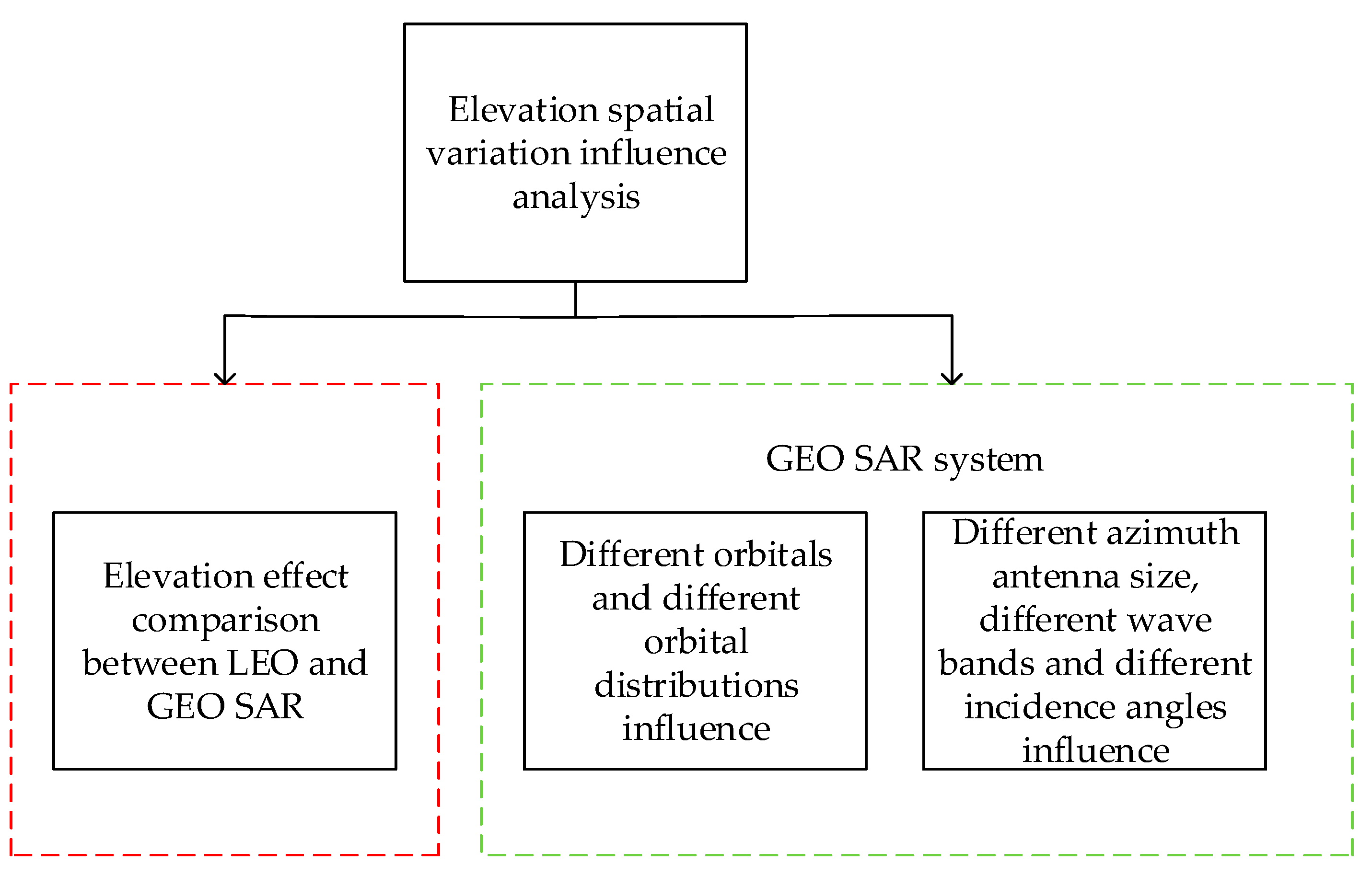
In this section, the difference of elevation influence between GEO SAR and LEO SAR is first analyzed, and the reason why elevation space variation is not necessary to be considered in LEO SAR is explained. Then, in the case of different orbital types, different position distributions on orbit, different azimuth antenna sizes, different wave bands and different incidence angles, the influences of target elevation on the overall phase error are analyzed. Figure 6 lists the factors mentioned above.
3.1. Elevation Effect Comparison Between LEO and GEO SAR
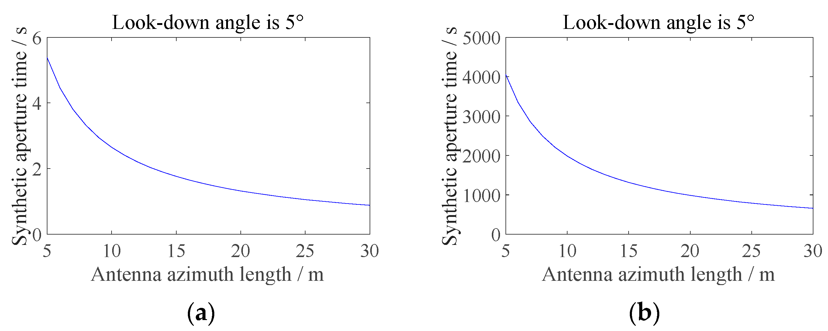
The difference between GEO SAR and LEO SAR is the satellite’s orbital altitude. GEO SAR has an orbital altitude of about 36,000 km. The paper will compare GEO SAR and LEO SAR with an orbit of 792 km to analyze the influence of elevation. The synthetic aperture time also varies due to the significant difference in orbital altitude. A new synthetic aperture time calculation method is proposed [27]. The variation trend of synthetic aperture time with antenna azimuth size in GEO SAR and LEO SAR is given below. In the following error analysis, if there is no special explanation for some parameters, system parameters are shown in Table 1.
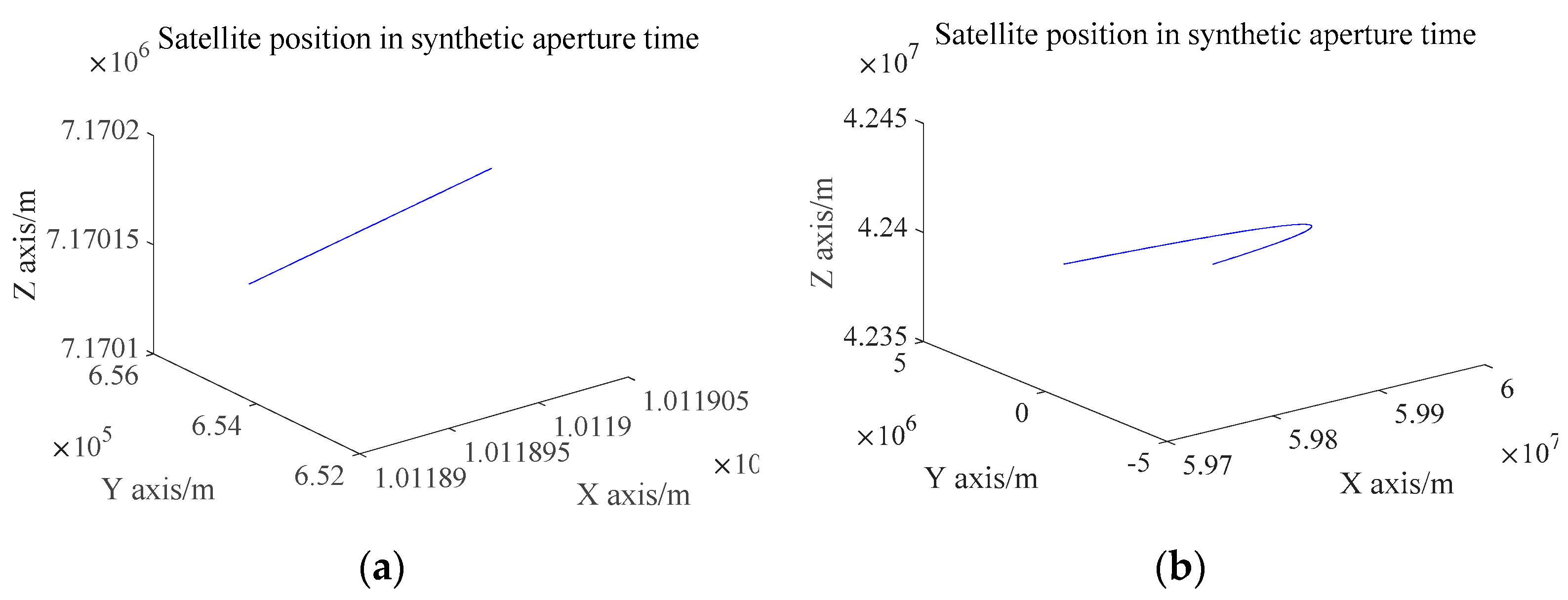
As can be seen from Figure 7 the synthetic aperture time is very short at low orbit, only a few seconds, whereas in the GEO system, the synthetic aperture time is thousands of seconds. Therefore, during the irradiation of the target, the curved flight trajectory of the satellite in the low orbit mode can be approximately regarded as linear motion, while the satellite trajectory in the GEO mode is ellipsoidal. Figure 8 shows the flight trajectories of satellites with a synthetic aperture time of 2 s in LEO mode and 2000 s in GEO mode, respectively:
It can be seen that in LEO SAR mode, the synthetic aperture time is very short, and the trajectory of the satellite when the target is irradiated is almost a straight line, while in GEO SAR, the trajectory is elliptical. It is precisely because the trajectory of the corresponding satellite in the synthetic aperture time is asymmetric about the zero Doppler plane that the corresponding point of the target at a certain elevation cannot be found, and the azimuth defocus is formed. The following theoretical analysis shows that LEO SAR can find a corresponding point while GEO SAR cannot find a corresponding point.
Firstly, it is assumed that there are corresponding points in both modes, and the slant range history geometric model of target and the corresponding point is as shown in Figure 2.
In the case of LEO SAR, referring to Figure 2, it is known that at moment , the distance between the target and the corresponding point to the satellite is equal, i.e. = . When the satellite runs to moment , according to the previous analysis, its trajectory is approximately linear, and the motion distance of the satellite can be seen as ; the distance between the target and the corresponding point to this satellite is and , and the range history can be calculated by the following formula:
In light of Equation (11), , such corresponding point does exist. The slant range history from the target to the satellite and from the corresponding point to the satellite are the same at different times.
In GEO mode, the orbit of the satellite is elliptical. Under these circumstances, the change of the satellite position with time cannot be treated as the linear trajectory approximation like the low-orbit mode, and the change of the position coordinates needs to be obtained through six orbital elements of the system: the elliptic orbit semi-major axis, orbital eccentricity, orbital inclination, right ascension of ascending, perigee and true anomaly. Assuming such corresponding points exist in GEO mode, the slant range history of target with a certain height and its corresponding point to the satellite can be obtained within the synthetic aperture time, as shown below:
where represents the satellite coordinate vector which changes with azimuth time in GEO mode, and can be obtained by six orbital elements. represents the slant range history from the corresponding point to the satellite. The orbit of the satellite calculated from the orbital element is ellipsoidal, and at the non-zero moment, there is a difference in the slant range history between and . The phase error caused by the difference in slant range history is:
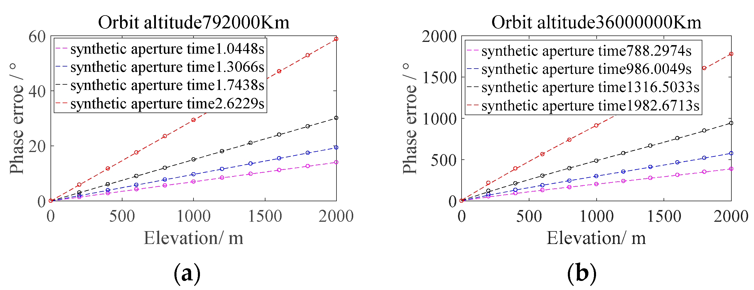
Then the variation trend of phase error between corresponding point and target with height is analyzed at different orbital altitudes (corresponding to different synthetic aperture times). The result is shown in Figure 9.
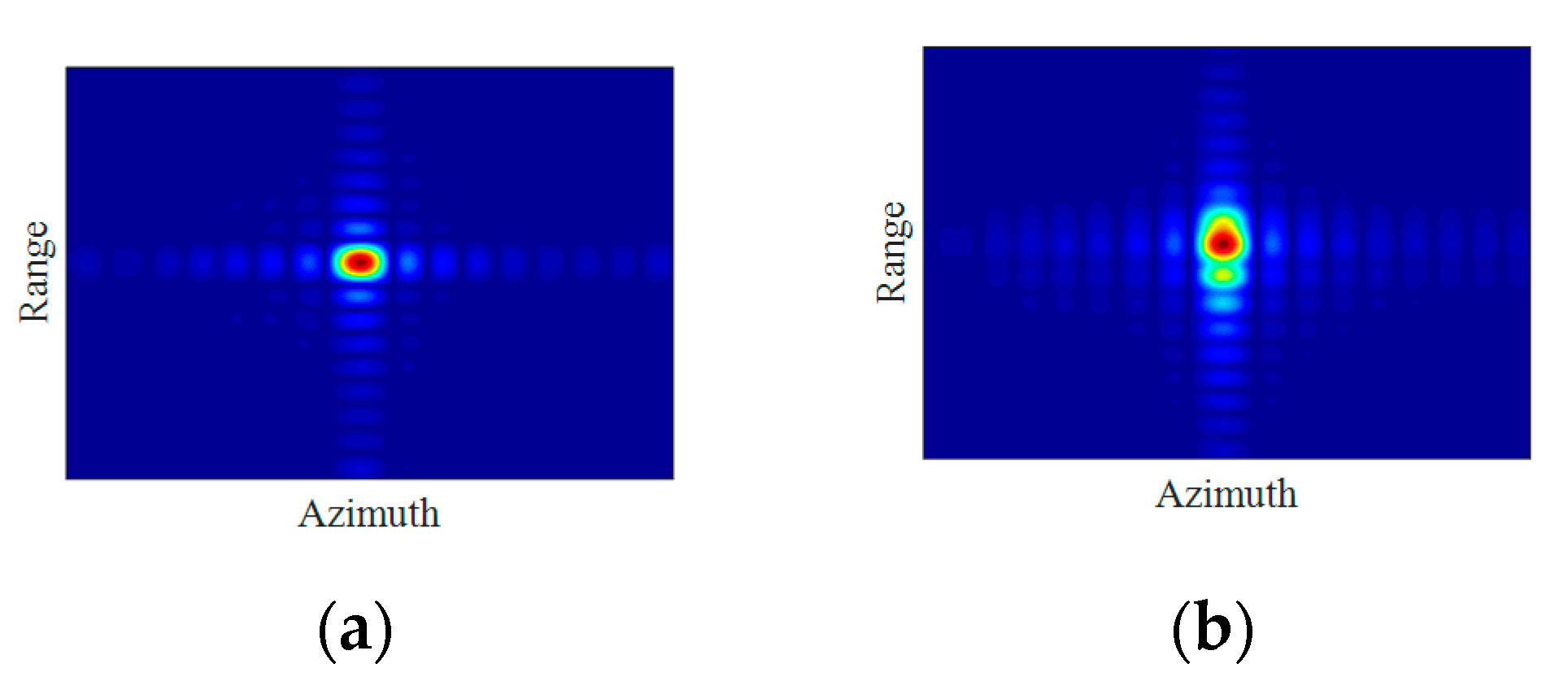
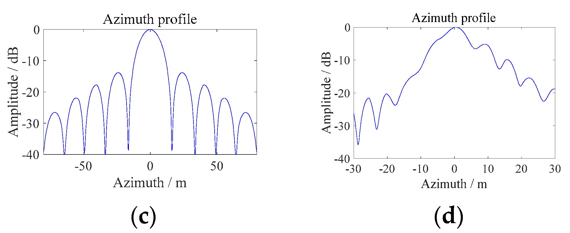
It can be seen that in LEO SAR mode, the phase error caused by elevation can almost be ignored, while in GEO SAR mode, the error is severe and will cause serious defocus of the imaging results. Additionally, there is a linear relationship between phase error and elevation. Figure 10 shows the imaging results and performance analysis of a point target with an altitude of 1800 m in two orbital modes:
As can be seen from Table 2, in the LEO mode, the error caused by elevation variation has almost no impact on the imaging, while in the GEO mode, the error will cause azimuth defocusing and seriously affect the imaging quality, which must be taken into consideration.
3.2. Influence of Orbit and Different Position Distributions on Orbits
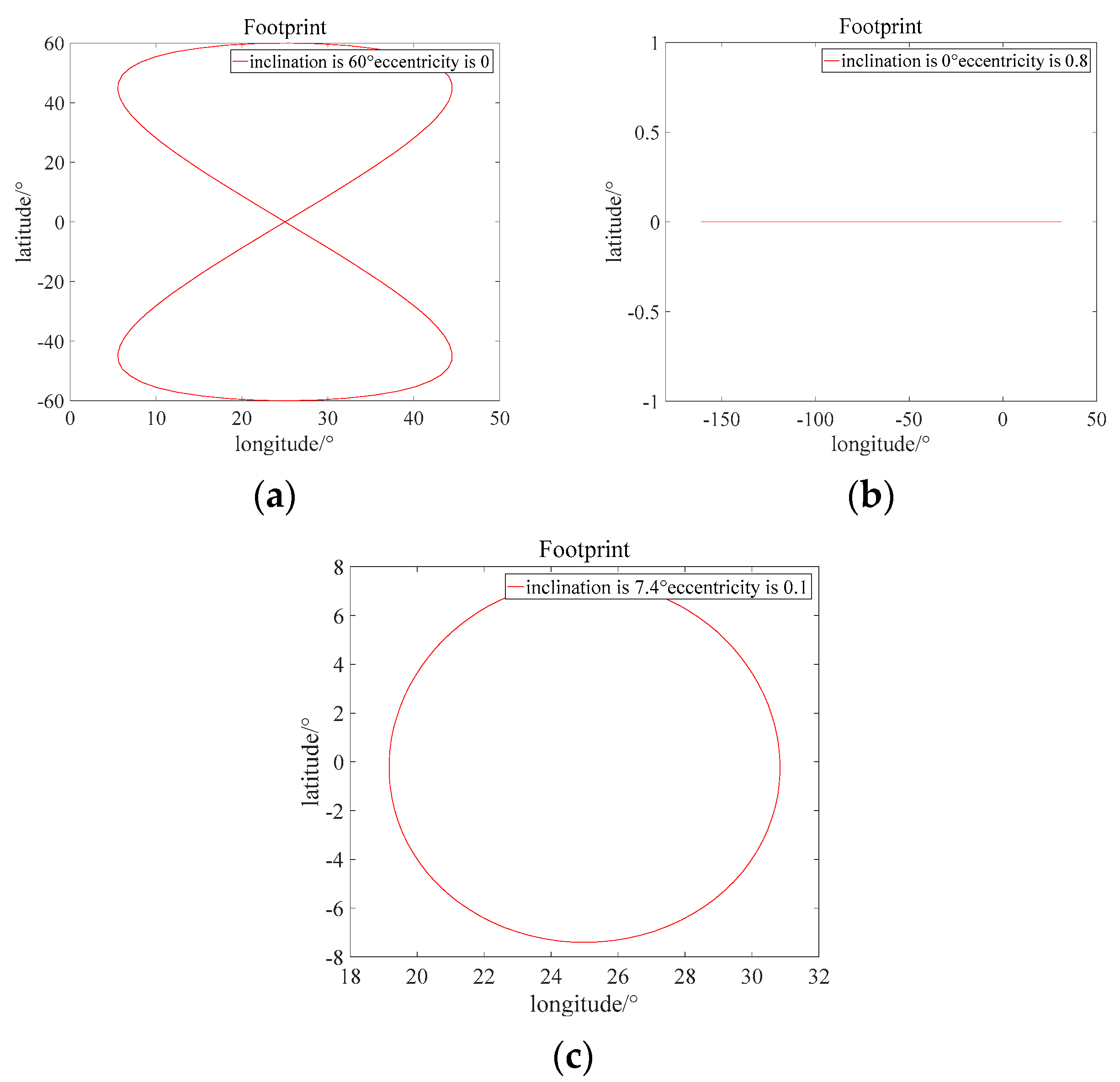
GEO SAR is a type of spaceborne SAR system in a geosynchronous orbit with a certain inclination and eccentricity with the typical footprints of type “–”, type “8” and type “O”. Changing the orbital inclination and eccentricity of the orbital parameters, i.e., setting the large orbital inclination and small orbital eccentricity, setting zero orbital inclination, and setting the small orbital inclination and large orbital eccentricity to obtain the typical footprints of type “8”, type “–” and type “O”, the results are shown in Figure 11. The parameters of the three orbits are shown in Table 3.
After obtaining different footprints, the influence of elevation on phase error under various orbits is analyzed, that is, the largest difference of phase history between the target and the corresponding point.
It can be seen from Figure 12 that the phase error in the “8”-shape orbit gradually increases with the target elevation. When the elevation is less than 336.9 m, the phase error is less than 45°, and the elevation spatial variation effect is light. In the shapes of “–” and “o”, the phase error also gradually increases with greater elevation, but the error between these two orbitals is very large compared to the “8”-shape track, and Figure 11 shows that these two kinds of orbit’s latitude coverage is small, not suitable for a wide swath of observation. Therefore, the rest of this study is focused on the “8”-shape track.
Now we analyze the effect of the elevation on the phase error at different locations in the orbit. There is a corresponding relationship between latitude argument and footprint, as shown in Figure 13. Perigee is set as 45°, and the true anomaly starts from 0° and increases by 45° in a total of 8 groups. Then, the phase error changes along with the elevation at several distribution positions marked in the orbit, as shown in Figure 14, are analyzed.
It can be seen from Figure 13 that the footprints in the shape of “8” are symmetric. Except for the two overlapping points at latitude = 0° (ω = 90° and ω = 270°), the errors of the other two points with the symmetry of longitude lines are the same. When ω = 360°, the footprints are located at the equator, and the phase error at this position is the smallest. It can be seen that the position is conducive to conducting some research on elevation direction. Therefore, the analysis following in this paper will set ω = 360° for research.
3.3. Influence of Different Azimuth Antenna Size, Different Wave Bands and Different Incidence Angles
It is well-known that the synthetic aperture time is affected by the azimuth antenna size, wavelength, and the incident angle [24]. Therefore, it is necessary to analyze the change of phase error with elevation under the influence of different azimuth antenna sizes, wavelengths and incident angles.
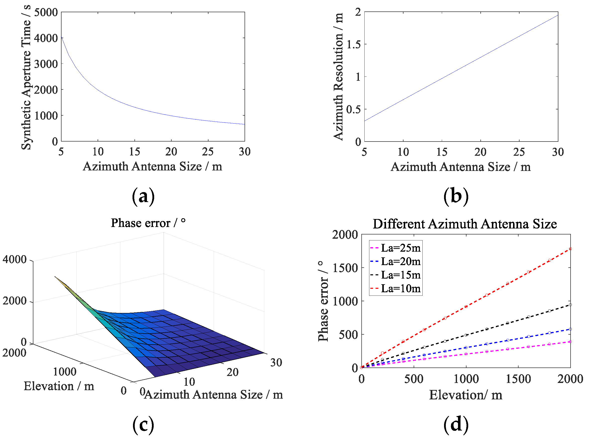
Firstly, the influence of antenna size on the elevation spatially variant error is analyzed. We also discuss the variation of the synthetic aperture time and azimuth resolution with the antenna size. Four sets of antenna sizes and four sets of elevation parameters were selected for direct analysis of the error variation curves with elevation and antenna sizes.
As can be seen from Figure 15, with the increase of antenna size, the azimuth resolution deteriorates. By comparing Figure 15a,e, it can be seen that with the increase of antenna size, synthetic aperture time becomes shorter and elevation spatial variation error also decreases. Since the antenna is between 5 and 15 m in size, the synthetic aperture time drops rapidly, so in order to reduce the complex elevation error compensation in some special cases (e.g., terrain elevation is small), the azimuth antenna can be set above 15 m. Therefore, the appropriate azimuth antenna size can be selected according to different requirements (the balance between resolution and elevation spatial variation error).
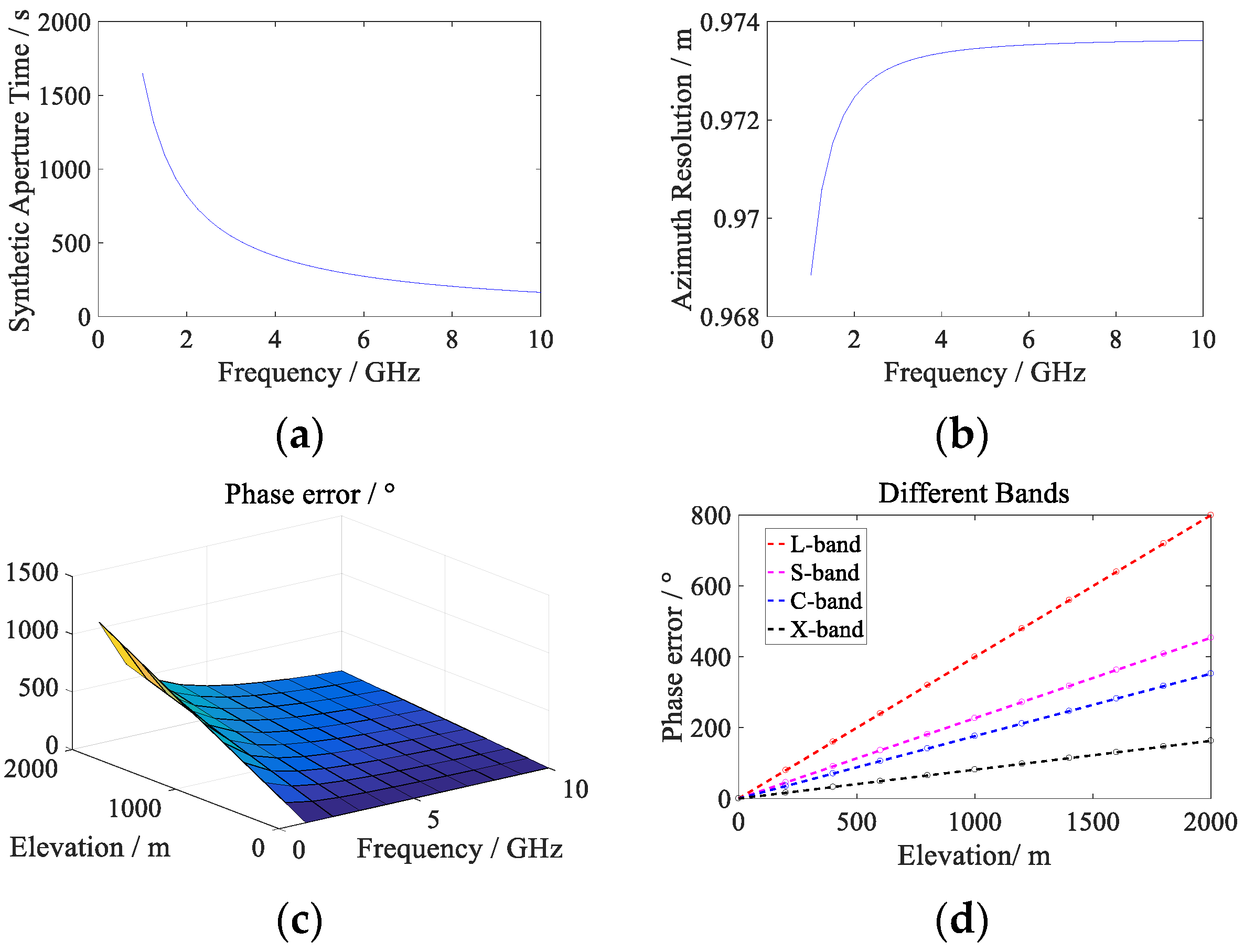
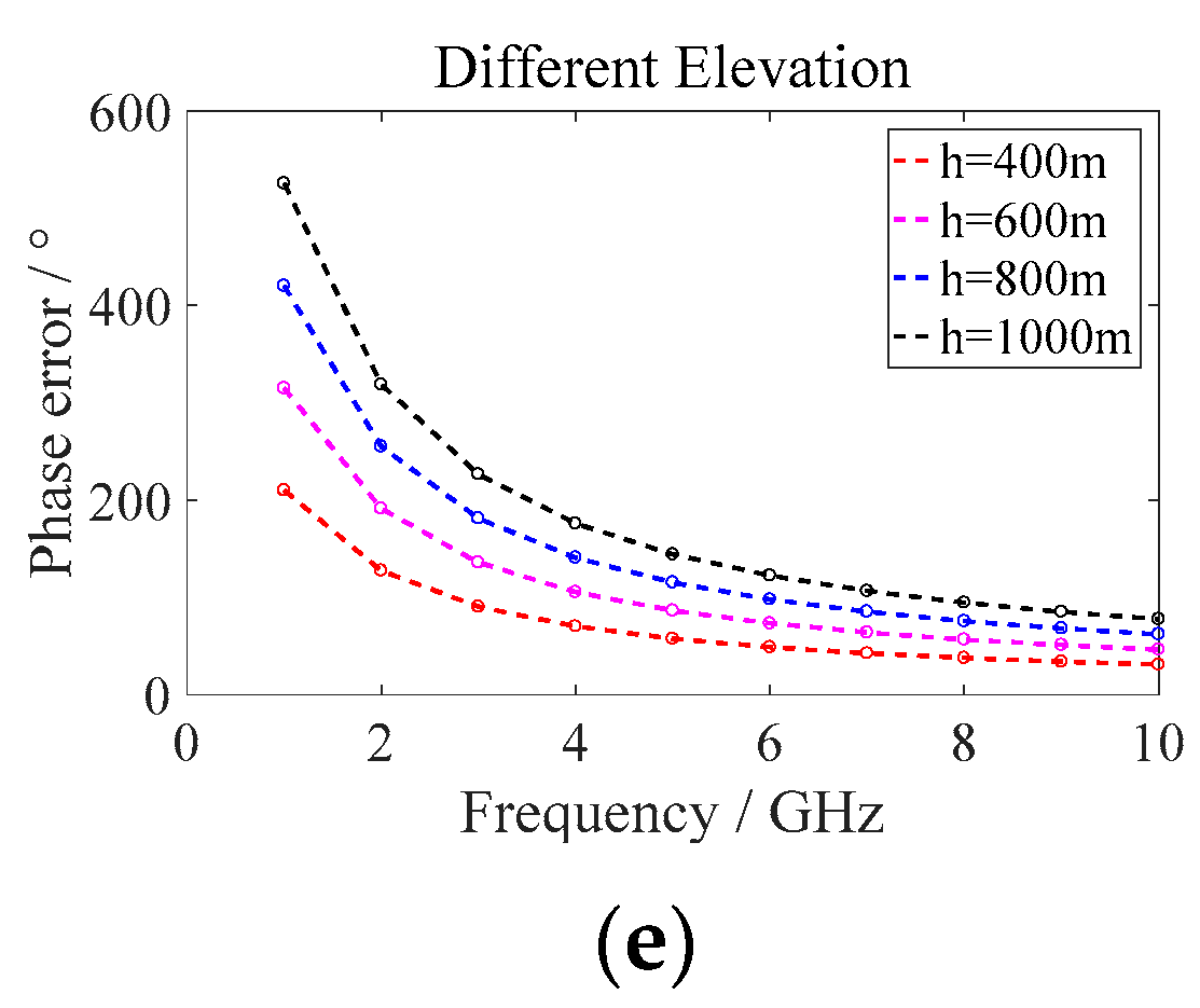
Next, we analyze how the synthetic aperture time and azimuth resolution vary with signal frequency, and how signal frequency and elevation affect the phase error. Four groups of common bands, namely, L band (1.5 GHz), S band (3 GHz), C band (4 GHz) and X band (9.5 GHz), and four groups of different elevations were set to get the change trend of phase error with elevation and frequency respectively.
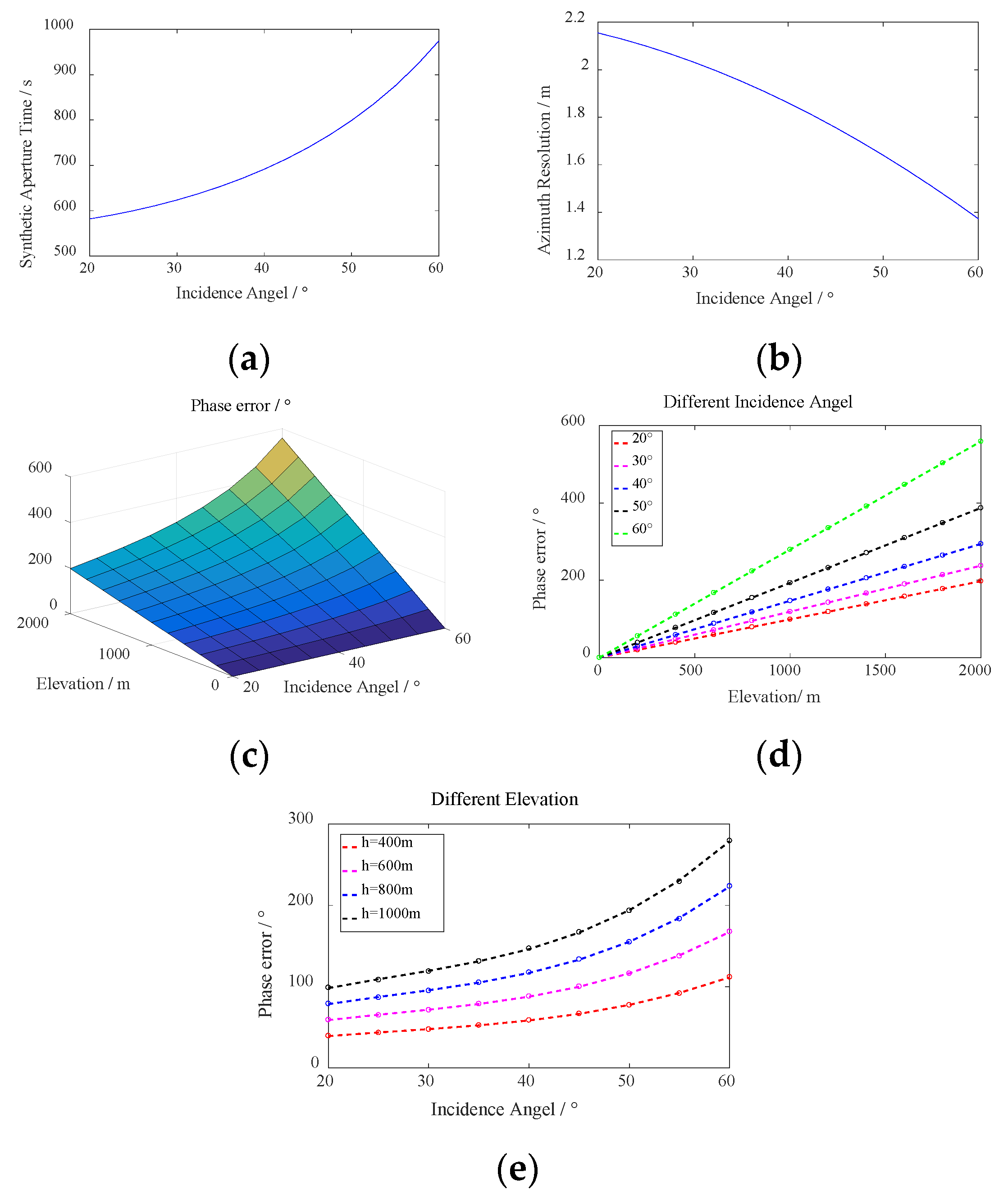
It can be seen from Figure 16 and the relation between wavelength and signal frequency that the longer wavelengths result in longer synthetic aperture time, better resolution and larger error. The phase error is proportional to the elevation and has a nonlinear relationship with the frequency. As can be seen from Figure 16e, within the frequency scope of 4 GHz, the error caused by elevation changes sharply with frequency, while over 4 GHz, the change is relatively gradual. In the process of system design, when the application demand is independent of terrain elevation and the elevation is small, the high-frequency band can be selected without considering the elevation space variation error. Now, let us analyze how the phase error varies with the incident angle. In GEO SAR systems, the ground incidence angle usually varies from 20° to 60°. Synthetic aperture time, azimuth resolution and phase error are also analyzed.
As can be seen from Figure 17, with the increase of incident angle, the synthetic aperture time becomes longer and the resolution performance becomes better, but the elevation spatial variation error will also increase, and the error has a linear relationship to the elevation instead of the incident angle. In GEO SAR imaging processing, when the elevation of the observed terrain is small, the elevation spatial variation error can be ignored by selecting the appropriate incident angle.
According to the previous analysis, the azimuth antenna size, transmitting signal wavelength and incident angle will affect the imaging resolution and elevation spatial variation error to a different extent. Relatively speaking, the signal wavelength has little effect on the resolution, while the antenna size is more sensitive. The incidence angle has little effect on the elevation variation error, while the error caused by the antenna size is much larger. At the same time, the variation trend of the synthetic aperture time and elevation spatial variation error is consistent. It can be concluded that the increase of synthetic aperture time leads to a larger error. In addition, elevation error increases linearly with elevation. Therefore, in future research, terrain elevation information can be retrieved through the linear relationship between the error and elevation in a signal image. In the orbit parameter design process of GEO SAR system, in order to make the observation swath larger, the “8”-shape orbit is generally selected, and in order to reduce the influence of elevation spatial variation error, the latitude argument is selected as 180° or 360°, so that the footprint falls near the equator. In the parameter design process of GEO SAR system, a balance can be chosen between the resolution requirement and the complexity of elevation error compensation processing to reasonably select the antenna size, wavelength and incident angle. If the imaging purpose requires high resolution, small antenna size, longer wavelength and larger incident angle can be selected, but elevation variation error compensation is also required. On the contrary, when the resolution requirement is not very high, correct selection can avoid the complex elevation variation error compensation processing and improve the imaging processing efficiency.
4. Elevation Spatial Variation Compensation Algorithm in GEO SAR Image Formation
In Section 2, starting from the original echo signal model of a single point target, we analyzed the influence of elevation in each decomposition phase of the signal from both qualitative and quantitative aspects, and proved the existence of elevation spatial variation. In GEO SAR imaging, 3D space variation seriously affects the depth of focus. In this part, the signal model within a scene considering spatial variation (range, azimuth and elevation spatial variation) is first established. Then the elevation spatial variation error is decomposed into range spatial variant error and azimuth time variant error. Finally, a new algorithm is proposed to improve the focusing depth.
4.1. Signal Model Considering Spatial Variation
In imaging processing, the first step is generally range compression, so the expression form of echo signal shown by Equation (1) after range compression is directly given here:
where represents the slant range history of the target, represents the slant range corresponding to the center moment, and represents the elevation of the target. Through high-order Taylor expansion, the fifth-order slant range model is generally accurate enough [28]. Compared with the second-order and third-order terms, the coefficient of elevation spatial variation of the fourth-order and fifth-order terms can be ignored. Therefore, the fifth-order slant range model is rebuilt as:
where and represents the 2D space variable coefficient and the elevation space variable coefficient. As and cause the variation of the Doppler central frequency. With the yaw steering, the values of which can be approximated to zeros. Therefore, the influences are also not considered. Compared with and , the influence of and is very weak, so we do not consider it. For a scene with known slope angle, since the height of the target is related to the position of the target, the elevation spatial variation can be decomposed into the 2D space variation of range and azimuth, as well as their coupling. Then, Equation (14) can be simplified as:
with
where represents the mixing spatial variation coefficient. According to the linear assumption, we model as:
where , and denotes range, azimuth and coupling space variation coefficient. The space variation coefficient in the above formulas can be obtained by fitting the 3D space variation model as shown in Figure 18. The detailed method was described in [28].
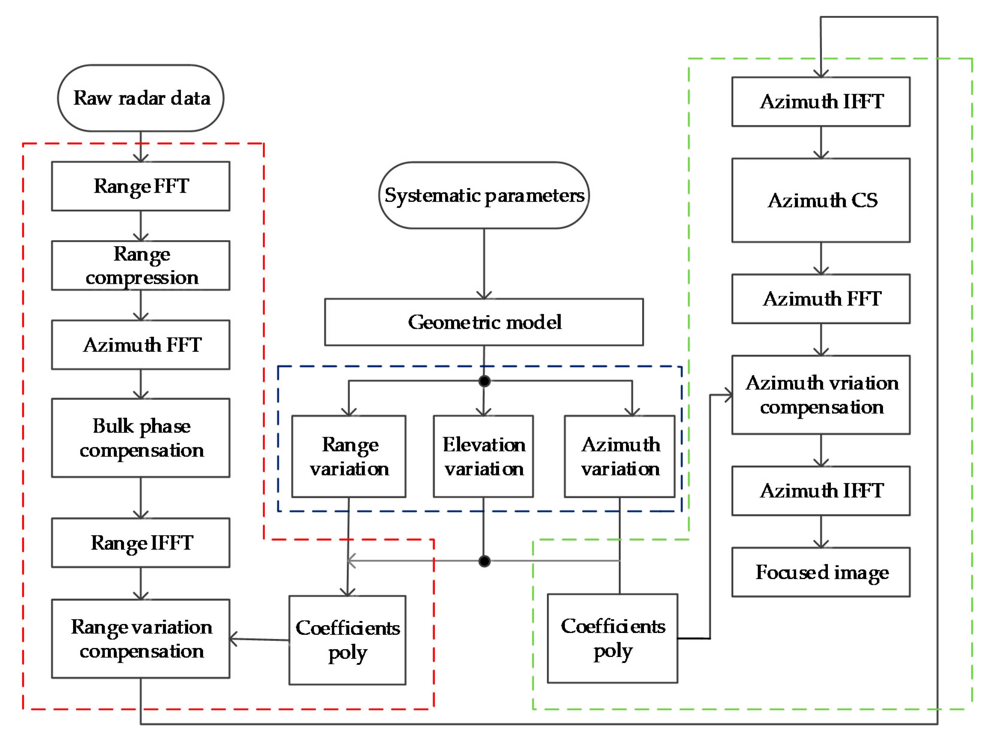
The algorithm flow chart for solving the 3D space change problem is shown in Figure 19.
4.2. Error Compensation
Firstly, bulk phase compensation is carried out, and the center point of the scene is taken as the reference point. The 2D spectrum of this point can be obtained through series reversion and POSP, and the echo data can be multiplied by the 2D spectrum of the reference point in the 2D frequency domain, followed by azimuth-backward compression. After bulk phase compensation, range and azimuth coupling can be removed. Next, the spatial variation of elevation is decomposed into range and azimuth, and the 3D space variation can be compensated in accordance with range spatial variation and azimuth time variation in turn.
The following is the compensation for range spatial variation. The coefficient of the high-order slant range model varies along with the range direction due to range and elevation spatial variation. In order to improve the focusing depth, this part of phase error should be compensated. After the bulk phase compensation, the range spatial variation is independent of the azimuth time variation, so it can be transformed into the range-Doppler domain.
By replacing in range migration and azimuth compression terms with , it can be obtained that:
where the subscript and represent range migration and azimuth compression. The residual range migration correction can be compensated by interpolation in the range-Doppler domain. Range spatially variant azimuth compression is also implemented in the range-Doppler domain.
After the range spatial variation compensation, the data are converted to the 2D time domain, then the azimuth time variant error is considered. Since the azimuth compression phase changes with azimuth time and azimuth frequency, azimuth time variant compensation cannot be realized directly in the range-Doppler domain as the range spatially variant compensation. Since we only need to consider the second- and third-order terms of the time-variant coefficients and they are linear, the azimuth chirp scaling can be introduced to deal with the problem [29,30]. The scaling function can be introduced, and the slant range model is:
Assuming and expanding , the formula can be rewritten as:
In the coefficient term of in Equation (21), the higher-order term of is very small and can be ignored unlike the constant term and the linear term. In order to achieve an azimuth-invariant slant range model, the linear terms of should be set to zeros, that is:
After completing the time domain compensation of azimuth time variation, the data are transferred to the range-Doppler domain, and the errors introduced by azimuth-compression phase and variable scale equation are compensated. The compensation phase can be obtained by using the series inversion and the POSP:
with
where phase represents the azimuth compression phase of the azimuth variation, and represents the stationary phase point. The azimuth variation compensation can be carried out in the range-Doppler domain, and the final inverse is achieved after the azimuth inverse fast Fourier transform. Thus, the correction of all spatial variation errors has been completed.
5. Simulation
The influence of the elevation spatial variation is analyzed in Section 3. In this part, the main purpose is to verify the correctness of the improved algorithm proposed to solve the spatial variation problem. The dot-matrix targets and distributed targets with elevation information are then analyzed.
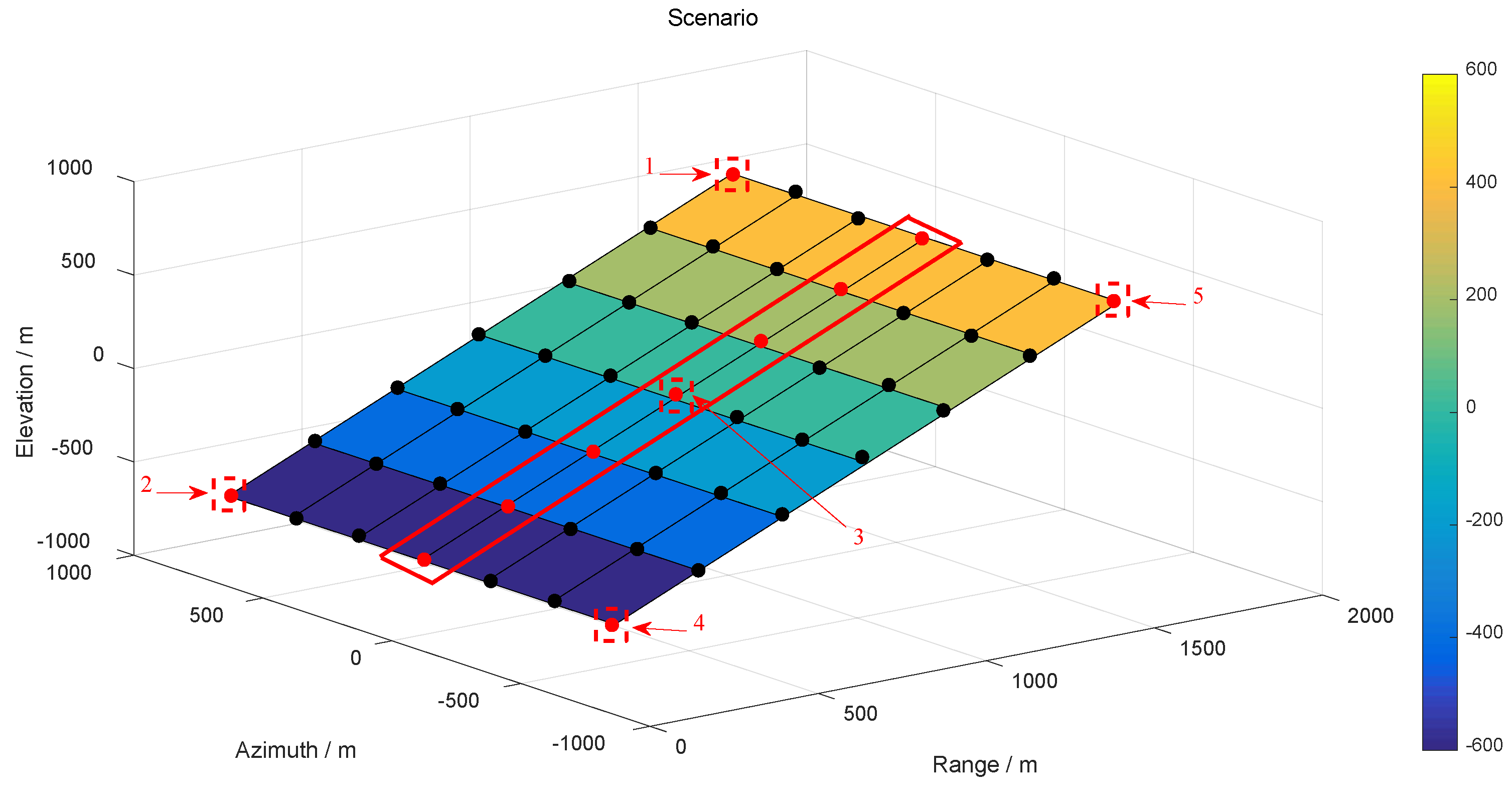
In order to verify the proposed improved RD-ACS algorithm, the scene slope angle was set as , and 7 × 7 dot-matrix targets were constructed. System parameters are shown in Table 1 of Section 3. The 3D scene and the improved RD-ACS imaging results are shown in the following figure.
The scenario is shown in Figure 20.
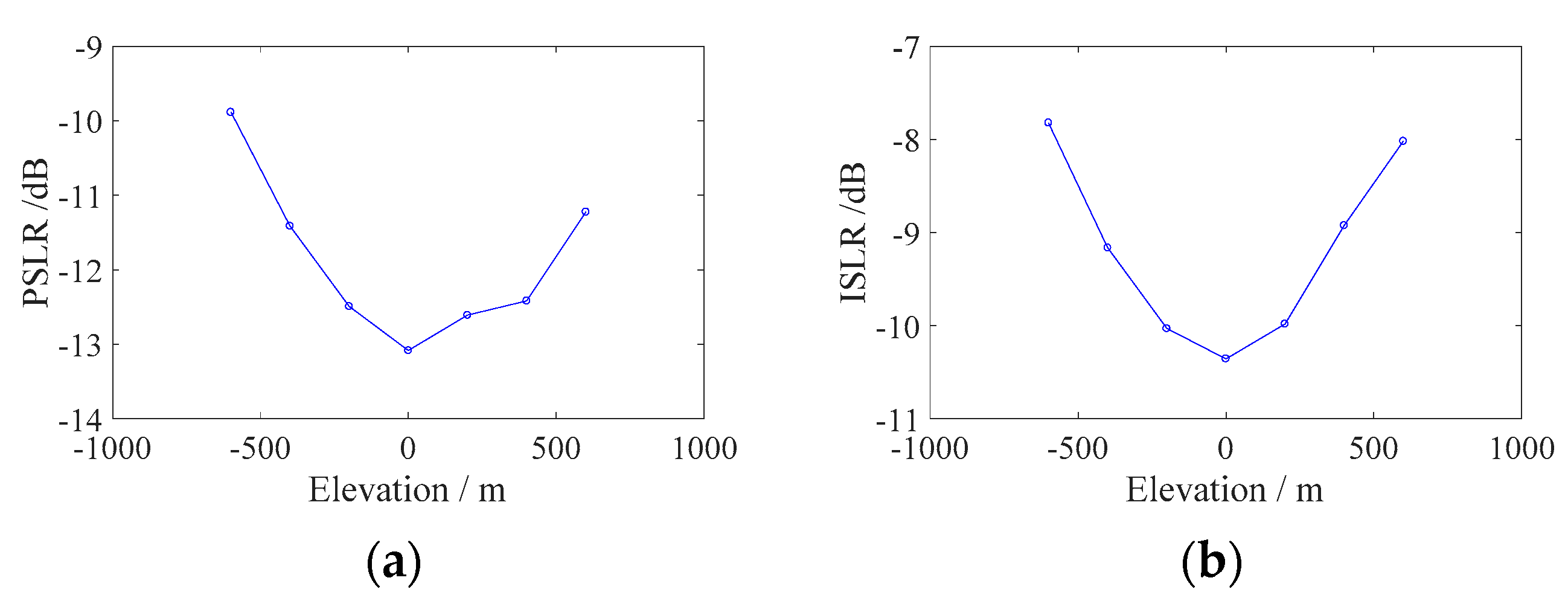
In order to reflect the existence of elevation spatial variation, the performance variation curves of different elevation points at zero azimuth moment in the imaging results of RD-ACS algorithm without considering elevation space variation are analyzed as shown in Figure 21 (7 points in the rectangular box with red solid line in Figure 20).
It can be seen from Figure 21 that the elevation spatial variation has a serious impact on azimuth focusing, and the error becomes more severe with the increase of the elevation, which is consistent with the previous analysis.
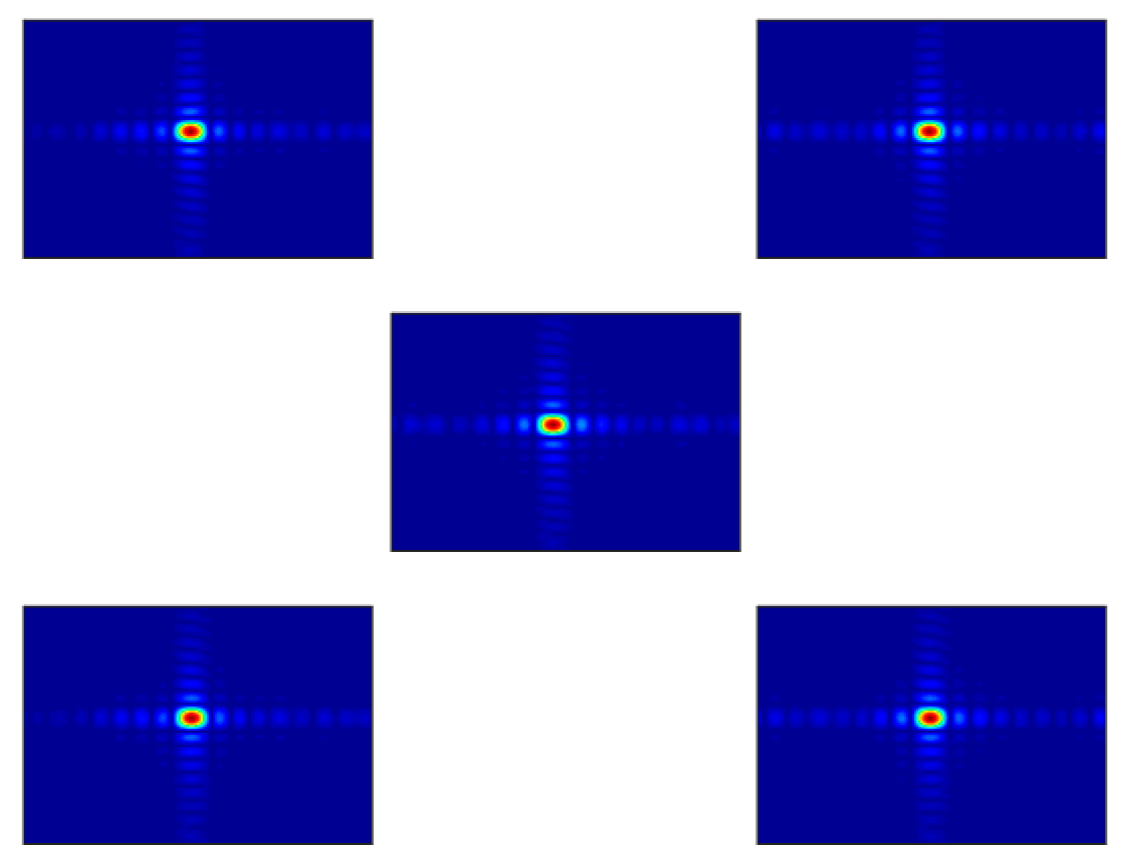
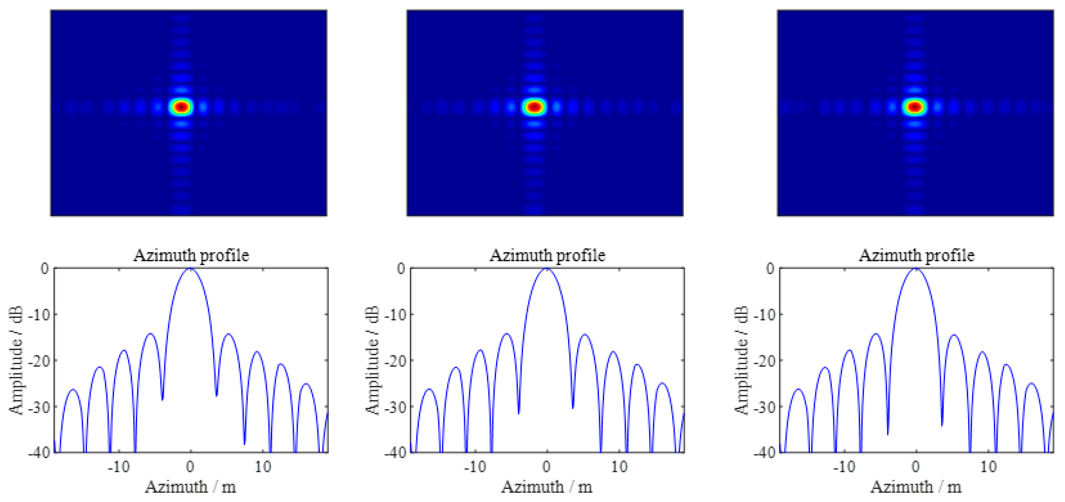
Next, five points (four points on the corner and center point have been marked 1–5, respectively, in Figure 20) are selected to show the details of the imaging results. The contour map of the points is shown in Figure 22.
The corresponding performance parameters of the five points are shown in the Table 4:
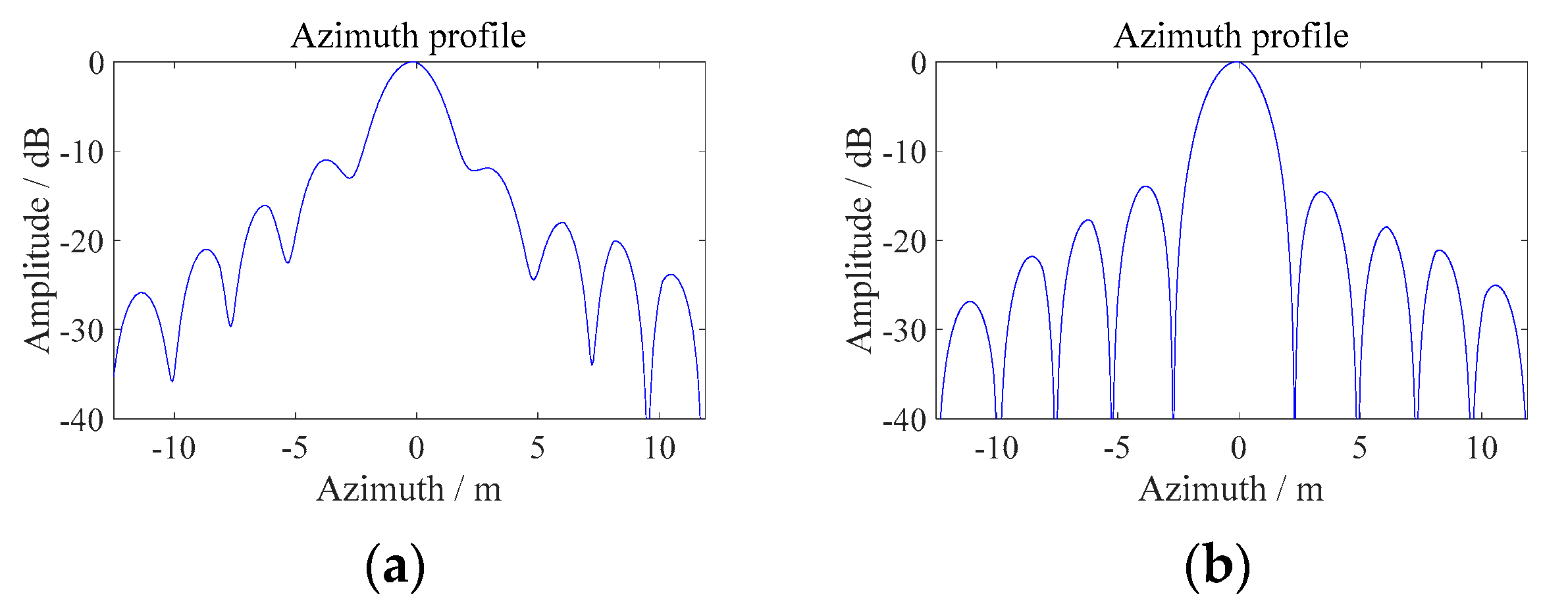
In order to further display the simulation results, the lower right corner point is selected to compare the azimuth profile of the two algorithms, as shown in the Figure 23:
According to the analysis of the dot-matrix targets, compared with RD-ACS algorithm, the proposed improved RD-ACS algorithm can well compensate the elevation spatially variant error and improve the focusing depth after the rough elevation information of the target is known. The following is an analysis of the distributed targets based on the point target, which is very necessary in the practical application of GEO SAR in the future.
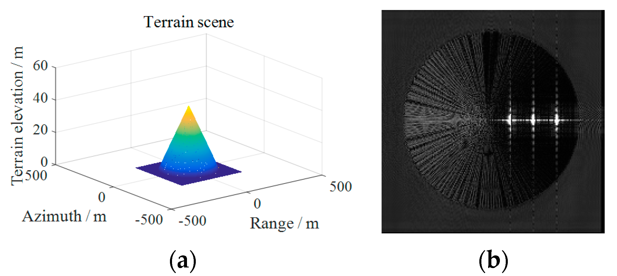
We first construct a slope, and place a small cone on the slope. Three strong scattering points (the heights of the three strong points on the cone are 36.1 m, 26.0 m and 15.8 m, and the height of the slope at the corresponding positions of the three points is 671.0 m, 654.6 m, and 692.2 m) are arranged on the cone and use the improved RD-ACS algorithm for imaging based on the slope, as the conical elevation is within the scope of negligible elevation spatially variant error. The azimuth antenna size is set to 45 m and the incident angle to 20°, and Table 1 can be consulted for the other parameters. The cone scene and the imaging results are shown in Figure 24.
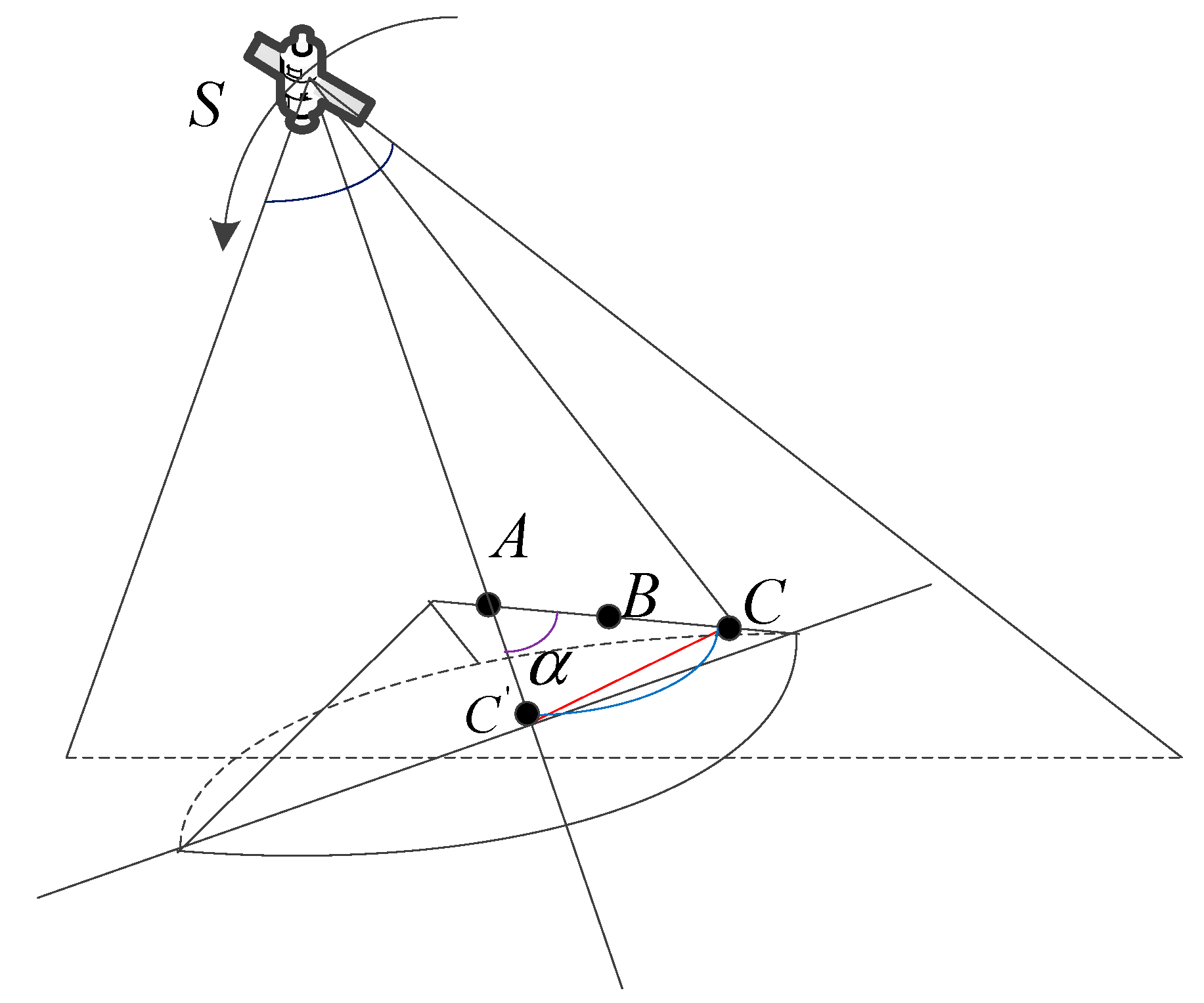
According to the geometric relationship between the satellite and the scattering points, as shown in Figure 25, the distance between the three points in the imaging results can be calculated according to Equation (25).
where represent the three points from left to right in Figure 24, represents the angle between and . The actual distance and in space are 140 m and 280 m, the distance calculated according to the formula in the image field is 21.2 m and 42.4 m in theory, and the distances calculated from the actual imaging results are 21.2 m and 42.4 m, as shown in Figure 24b. Therefore, due to the existence of the target elevation information, the distance of the scattering points in the image domain is shortened compared with the actual distance in space. Then, the imaging results of the three strong scattering points are shown in Figure 26. The performance parameters of the three strong scattering points are shown in Table 5.
It can be seen that the imaging results of the improved algorithm have a good focusing effect for the distributed targets with elevation information.
6. Discussion
In the future practical application of GEO SAR systems, it is inevitable to image the target with elevation information. In previous analyses, it has been explained in detail that elevation can cause severe defocus of the image results. To solve the problem, we propose an algorithm to compensate the elevation spatially variant error for the general slope plane scene. Therefore, in Section 5, we carried out simulation experiments to validate the compensation effect of the algorithm. We first set the dot-matrix targets on the slope, so that each point has a different elevation information. The RD-ACS algorithm which can compensate for 2D space variation of range and azimuth can be used for imaging. By drawing the variation curve of performance parameters (PSLR and ISLR) with elevation (as shown in Figure 21), it can be seen that elevation information causes serious azimuth defocus of imaging results, and the defocus effect becomes more serious as the elevation increases. As a comparison, the improved RD-ACS algorithm proposed was used for imaging again, and five points were selected for analysis. The imaging results are shown in Figure 22. Additionally, the performance parameters of these five points are analyzed, as shown in Table 4. It can be seen that the focus result of the improved algorithm is excellent, and the performance has been significantly improved compared with the previous one. Then, on the basis of the point targets, the distributed targets are also analyzed by placing a small cone on the slope (within the scope of negligible elevation spatial variation). Similar to the analysis process of point targets, three strong scattering points are set on the cone as the research object. By comparing the 3D space distance between the three points, it can be seen that the distance in the image domain will decrease due to the existence of elevation information. From the imaging results and performance parameter analysis of these three points, it can be seen that the improved RD-ACS algorithm has a fine compensation effect. Finally, although the simulations for both point targets and distributed targets can prove the feasibility and advantage of the proposed improved RD-ACS method, there are some shortcomings and limitations too, which will be explained and discussed in detail in the next section.
7. Conclusions
This paper mainly studies the influence and compensation algorithm of elevation spatial variation. Firstly, we set up a geometric model considering the elevation spatial variation. From the original echo signal, we analyzed the influence of elevation on the echo and the subsequent imaging processing qualitatively and quantitatively. In the 2D spectrum of echo signal, the effect of elevation on each decomposed phase was analyzed. It is concluded that the azimuth compression phase is greatly affected by the elevation and the range migration phase is almost not affected, but this error is still taken into account in the compensation. Secondly, the effect of elevation in LEO SAR and in GEO SAR is compared, and the conclusion is drawn that the elevation space variation error can be ignored under low orbit. In addition, the influence of elevation spatial variation of typical footprints in GEO SAR system is studied. It is concluded that the “8” type orbit not only covers a large observation area, but also has the least influence on elevation spatial variation compared with the other two kinds of footprints, and when the footprint is located at the equator, it has the least influence on elevation. Therefore, we choose the most common Figure 8 orbit and take the latitude argument of 360° as the research object. The influence of azimuth antenna size, wavelength and incident angle on elevation variation error and resolution was analyzed, which is beneficial to design system parameters according to actual needs. For example, by selecting the appropriate parameters just mentioned, the elevation spatially variant error can be ignored for targets with small height. Thirdly, an improved algorithm is proposed to solve the elevation spatially variant error and improve the focusing depth. The algorithm is applicable not only to smooth slope but also to slope with slowly variant part, as the elevation spatial variation can be ignored in a small elevation scope. Finally, the correctness of the algorithm is verified by point targets and distributed targets in the experiment part.
The analysis in this paper can provide a theoretical basis for the future design of GEO SAR systems, and the improved imaging algorithm can be used to improve the focusing depth of scenes containing rough elevation information. However, this algorithm is only applicable to the general slope scene, and it cannot compensate for the elevation spatial variation for those complex scenes with fast variant parts. In future research, we will focus on the study of high-resolution imaging of complex scenes. An arbitrarily complex scene can be divided into two parts, namely, the slope and the fast variant part. The imaging algorithm proposed in this paper is used to carry out rough imaging of the slowly variant slope, and for the remaining part, the spatial variation error caused by fast variant part is compensated by the method of autofocus. Then the height of the target is inverted by using the relationship between the error and the height, as mentioned in Section 3. This work will have greater significance in practical engineering.
Author Contributions
All authors have made substantial contributions to this work. F.C. and D.L. formulated the theoretical framework. F.C., Z.H. and D.L. designed the simulations; F.C. carried out the simulation experiments. F.C., D.L. and Z.D. analyzed the simulated data. F.C. wrote the manuscript. D.L., X.C., Y.H. and Z.D. reviewed and edited the manuscript. Z.D. gave insightful and enlightening suggestions for this manuscript. All authors have read and agreed to the published version of the manuscript.
Funding
This research received no external funding.
Data Availability Statement
The data presented in this study are available on request from the corresponding author.
Acknowledgments
The authors would like to thank all those who gave valuable help and suggestions to this manuscript, which were essential to the outcome of this paper.
Conflicts of Interest
The authors declare no conflict of interest.
Appendix A
The expression of the stationary phase point obtained by series inversion is as follows:
The parameter definitions in the above formulas can be referred to the paper.
Appendix B
The 2D spectrum decomposition phase of the fifth-order slant range model echo.
The parameter definitions in the above formulas can be referred to in the paper.
References
- DLR. Terra SAR-X Ground Segment Basic Product Specification Document; TX-GS-DD-3302; German Aerospace Center: Cologne, Germany, 2010. [Google Scholar]
- Prats, P.; Scheiber, R.; Marotti, L.; Wollstadt, S.; Reigber, A. TOPS interferometry with Terra SAR-X. IEEE Trans. Geosci. Remote Sens. 2012, 50, 3179–3188. [Google Scholar] [CrossRef] [Green Version]
- Tomiyasu, K. Synthetic aperture radar in geosynchronous orbit. In Proceedings of the Digest International IEEE Antennas Propagation Symposium, College Park, MD, USA, 15–19 May 1978; pp. 42–45. [Google Scholar]
- Tomiyasu, K. Synthetic Aperture Radar Imaging from an Inclined Geosynchronous Orbit. IEEE Trans. Geosci. Remote Sens. 1983, 21, 324–329. [Google Scholar] [CrossRef]
- Cutrona, L.; Skolnik, M. Radar Handbook; McGraw-Hill: New York, NY, USA, 1970. [Google Scholar]
- Cazzani, L.; Colesanti, C.; Leva, D.; Nesti, G.; Prati, C.; Rocca, F.; Tarch, D. A ground-based parasitic SAR experiment. IEEE Trans. Geosci. Remote Sens. 2000, 38, 2132–2141. [Google Scholar] [CrossRef]
- Erik, M. Handbook of Geostationary Orbits, 1st ed.; Kluwer Academic Publishers: Amsterdam, The Netherlands, 1994; pp. 886–1070. [Google Scholar]
- Bruno, D.; Hobbs, S. Radar imaging from geosynchronous orbit: Temporal decorrelation aspects. IEEE Trans. Geosci. Remote Sens. 2010, 48, 2924–2929. [Google Scholar] [CrossRef]
- Kempf, T.; Anglberger, H.; Suess, H. Depth-of-Focus Issues on Spaceborne very High Resolution SAR. In Proceedings of the 2012 IEEE International Geoscience and Remote Sensing Symposium, Munich, Germany, 22–27 July 2012; pp. 7448–7451. [Google Scholar]
- Rodriguez-Cassola, M.; Prats-Iraola, P.; De Zan, F.; Scheiber, R.; Reigber, A. Doppler-related focusing aspects in the TOPS imaging mode. In Proceedings of the IEEE International Geoscience and Remote Sensing Symposium (IGARSS), Melbourne, Australia, 21–26 July 2013. [Google Scholar]
- Macedo, K.; Scheiber, R. Precise topography- and aperture-dependent motion compensation for airborne SAR. IEEE Geosci. Remote Sens. Lett. 2005, 2, 172–176. [Google Scholar]
- Blacknell, D.; Freeman, A.; Quegan, S.; Ward, I.; Finley, I.; Oliver, C.; White, R.; Wood, J. Geometric accuracy in airborne SAR images. IEEE Trans. Aerosp. Electron. Syst. 1989, 25, 241–258. [Google Scholar] [CrossRef]
- Duque, S.; Breit, H.; Balss, U.; Parizzi, A. Absolute height estimation using a single Terra SAR-X staring spotlight acquisition. IEEE Geosci. Remote Sens. Lett. 2015, 12, 1735–1739. [Google Scholar] [CrossRef] [Green Version]
- Prats, P.; Scheiber, R.; Rodriguez, M. On the Processing of Very High Resolution Spaceborne SAR Data. IEEE Trans. Geosci. Remote Sens. 2014, 52, 6003–6015. [Google Scholar] [CrossRef] [Green Version]
- Prats, P.; Macedo, K.; Reigber, A.; Scheiber, R.; Mallorqui, J. Comparison of topography- and aperture-dependent motion compensation algorithms for airborne SAR. IEEE Geosci. Remote Sens. Lett. 2007, 4, 349–353. [Google Scholar] [CrossRef] [Green Version]
- Hu, B.; Jiang, Y.; Zhang, Y.; Yeo, T. Accurate slant range model and focusing method in geosynchronous SAR. In Proceedings of the 2015 IEEE International Geoscience and Remote Sensing Symposium (IGARSS), Milan, Italy, 26–31 July 2015; pp. 4464–4467. [Google Scholar]
- Zhang, Q.; Yin, W.; Ding, Z. An Optimal Resolution Steering Method for Geosynchronous Orbit SAR. IEEE Geosci. Remote Sens. Lett. 2014, 11, 1732–1736. [Google Scholar] [CrossRef]
- Wu, X.; Zhang, S.; Xiao, B. An advanced equivalent slant range model and image formation in geosynchronous SAR. In Proceedings of the 2012 International Workshop on Microwave and Millimeter Wave Circuits and System Technology, Chengdu, China, 19–20 April 2012; pp. 1–4. [Google Scholar]
- Hu, B.; Jiang, Y.; Zhang, S.; Zhang, Y. Generalized omega-K algorithm for geosynchronous SAR image formation. IEEE Geosci. Remote Sens. Lett. 2015, 12, 2286–2290. [Google Scholar] [CrossRef]
- Geng, J.; Yu, Z.; Li, C.; Wei, L. Squint Mode GEO SAR Imaging Using Bulk Range Walk Correction on Received Signals. Remote. Sens. 2019, 11, 17. [Google Scholar] [CrossRef] [Green Version]
- Li, Z.; Li, C.; Yu, Z.; Zhou, J.; Chen, J. Back projection algorithm for high resolution GEO-SAR image formation. In Proceedings of the 2011 IEEE International Geoscience and Remote Sensing Symposium, Vancouver, BC, Canada, 24–29 July 2011; pp. 336–339. [Google Scholar]
- Neo, Y.; Wong, F.; Cumming, I. A Two-Dimensional Spectrum for Bistatic SAR Processing Using Series Reversion. IEEE. Geosci. Remote Sens. Lett. 2007, 4, 93–96. [Google Scholar] [CrossRef]
- Zhu, Y.; Ke, M.; Zhang, T.; Li, G.; Ding, Z. Image Representation of GEO SAR Time-Variant Scene. In Proceedings of the 12th European Conference on Synthetic Aperture Radar, Aachen, Germany, 4–7 June 2018; pp. 1–5. [Google Scholar]
- Li, D.; Zhu, X.; Dong, Z.; Yu, A.; Zhang, Y. Background Tropospheric Delay in Geosynchronous Synthetic Aperture Radar. Remote. Sens. 2020, 12, 3081. [Google Scholar] [CrossRef]
- Curlander, J.; McDonough, R. Synthetic Aperture Radr: Systems and Signal Processing; John Wiley Sons: New York, NY, USA, 1991. [Google Scholar]
- Feng, H.; Qi, C.; Zhen, D.; Guang, J.; Dian, L. Modeling and high-precision processing of the azimuth shift variation for spaceborne HRWS SAR. Sci. China Inf. Sci. 2012, 56, 1–12. [Google Scholar] [CrossRef] [Green Version]
- Li, D.; Wu, M.; Sun, Z.; He, F.; Dong, Z. Modeling and Processing of Two-Dimensional Spatial-Variant Geosynchronous SAR Data. IEEE J. Sel. Top. Appl. Earth Obs. Remote Sens. 2015, 8, 3999–4009. [Google Scholar] [CrossRef]
- Hu, C.; Tao, Z. The accurate resolution analysis in Geosynchronous SAR. In Proceedings of the 8th European Conference on Synthetic Aperture Radar, Aachen, Germany, 7–10 June 2010; pp. 925–928. [Google Scholar]
- Wong, F.; Cumming, I.; Neo, Y. Focusing Bistatic SAR Data Using the Nonlinear Chirp Scaling Algorithm. IEEE Trans. Geosci. Remote Sens. 2008, 46, 2493–2505. [Google Scholar] [CrossRef] [Green Version]
- An, H.; Wu, J.; Sun, Z.; Yang, J. A two-step nonlinear chirp scaling method for multichannel GEO spaceborne-airborne bistatic SAR spectrum reconstructing and focusing. IEEE Trans. Geosci. Remote Sens. 2019, 57, 16. [Google Scholar] [CrossRef]
Figure 1.
The block diagram of the GEO SAR geometry and signal models.

Figure 2.
Slant range history diagram in GEO SAR.

Figure 3.
The variation of phase error with elevation caused by the different slant range model as the slant range course of the target. (a) Second-order slant range model in the LEO system. (b) Fifth-order slant range model in the LEO system. (c) Second-order slant range model in the GEO system. (d) Fifth-order slant range model in the GEO system.

Figure 4.
Decomposed phase error at five groups of elevation. (a) Azimuth compression phase error varies with azimuth frequency. (b) Range migration phase error varies with azimuth frequency. (c) Magnification of the middle curve selected in (b). (d) Range migration phase error varies with range frequency. (e) Residual phase error varies with elevation. (f) Effective velocity varies with elevation.

Figure 5.
Decomposed phase error at five groups of elevation: (a) Azimuth compression phase error varies with azimuth frequency. (b) Range migration phase error varies with azimuth frequency. (c) Range migration phase error varies with range frequency. (d) Residual phase error varies with elevation. (e) Effective velocity varies with elevation.

Figure 6.
Block diagram of elevation spatial variation influence.

Figure 7.
Synthetic aperture time variation trend. (a) LEO Mode. (b) GEO Mode.

Figure 8.
Satellite trajectories. (a) LEO Mode. (b) GEO Mode.

Figure 9.
(a) LEO Mode phase error. (b) GEO Mode phase error.

Figure 10.
(a,c) LEO Mode imaging result. (b,d) GEO Mode imaging result.


Figure 11.
Different footprints. (a) Type “8” orbit. (b) Type “–” orbit. (c) Type “o” orbit.

Figure 12.
Phase error under different footprints. (a) Type “8” orbit. (b) Type “-” orbit. (c) Type “o” orbit.
Figure 12.
Phase error under different footprints. (a) Type “8” orbit. (b) Type “-” orbit. (c) Type “o” orbit.

Figure 13.
Different distribution on the footprint of type “8”.

Figure 14.
(a–h) represent the curve of the phase error at different latitude argument on the orbit along with the elevation.
Figure 14.
(a–h) represent the curve of the phase error at different latitude argument on the orbit along with the elevation.


Figure 15.
(a) Synthetic aperture time varies with antenna size. (b) Azimuth resolution varies with antenna size. (c) Phase error varies with elevation and antenna size. (d) Phase error varies with elevation at different antenna sizes. (e) Phase error varies with antenna size at different elevations.


Figure 16.
(a) Synthetic aperture time varies with signal frequency. (b) Azimuth resolution varies with signal frequency. (c) Phase error varies with elevation and signal frequency. (d) Phase error varies with elevation at different wavelengths. (e) Phase error varies with signal frequency at different elevations.


Figure 17.
(a) Synthetic aperture time varies with incident angle. (b) Azimuth resolution varies with incident angle. (c) Phase error varies with elevation and incident angle. (d) Phase error varies with elevation at different incident angles. (e) Phase error varies with incident angle at different elevations.

Figure 18.
3D space variable geometric model.

Figure 19.
Algorithm flow for 3D space variation compensation in GEO SAR imaging.

Figure 20.
Schematic diagram of 3D slope scene.

Figure 21.
(a) PSLR curve. (b) ISLR curve.

Figure 22.
Imaging results.

Figure 23.
Imaging results comparison. (a) RD-ACS algorithm. (b) Improved algorithm.

Figure 24.
(a) Cone scenario. (b) Imaging result.

Figure 25.
Geometrical model between satellite and scattering points.

Figure 26.
Imaging results.


Table 1.
System parameters.
| Parameter | Value | Parameter | Value |
|---|---|---|---|
| Semi-major axis | 42,164.17 km | Right ascension of ascending | 115° |
| Eccentricity | 1 × 10⁻⁸ | Perigee | 270° |
| Orbital inclination | 60° | True anomaly | 90° |
| Carrier frequency | 1.25 GHz | Antenna size | 30 m × 30 m |
| Squint angle | 0° | Incident angle | 35.2° |
| Pulse duration | 2.5 μs | Chirp bandwidth | 30 MHz |
Table 2.
Performance parameters.
| Mode | Main Lobe Broadening | PSLR/dB | ISLR/dB |
|---|---|---|---|
| LEO | 1.0625 | −13.9454 | −10.9699 |
| GEO | 1.4375 | −5.1536 | −6.0431 |
Note: PSLR, peak side lobe ratio; ISLR, integral side lobe ratio.
Table 3.
System parameters.
| Orbital Parameters | Type “8” | Type “–” | Type “O” |
|---|---|---|---|
| Inclination | 60° | 0° | 7.4° |
| Eccentricity | 0 | 0.1 | 0.1 |
| Perigee | 270° | 270° | 270° |
Table 4.
Performance parameters.
| Point | Resolution (m) | PSLR (dB) | ISLR (dB) |
|---|---|---|---|
| 1 | 2.0914 | −13.1584 | −10.2438 |
| 2 | 2.0931 | −13.1452 | −10.2164 |
| 3 | 2.0903 | −13.2334 | −10.3586 |
| 4 | 2.0910 | −13.1576 | −10.2746 |
| 5 | 2.0907 | −13.1895 | −10.2300 |
Table 5.
Performance parameters.
| Point | Resolution (m) | PSLR (dB) | ISLR (dB) |
|---|---|---|---|
| A | 3.1385 | −13.0990 | −10.3013 |
| B | 3.1385 | −13.0193 | −10.3614 |
| C | 3.1385 | −13.1243 | −10.4115 |
Publisher’s Note: MDPI stays neutral with regard to jurisdictional claims in published maps and institutional affiliations. |
© 2021 by the authors. Licensee MDPI, Basel, Switzerland. This article is an open access article distributed under the terms and conditions of the Creative Commons Attribution (CC BY) license (https://creativecommons.org/licenses/by/4.0/).
Share and Cite
MDPI and ACS Style
Chang, F.; Li, D.; Dong, Z.; Huang, Y.; He, Z.; Chen, X. Elevation Spatial Variation Analysis and Compensation in GEO SAR Imaging. Remote Sens. 2021, 13, 1888. https://0-doi-org.brum.beds.ac.uk/10.3390/rs13101888
AMA Style
Chang F, Li D, Dong Z, Huang Y, He Z, Chen X. Elevation Spatial Variation Analysis and Compensation in GEO SAR Imaging. Remote Sensing. 2021; 13(10):1888. https://0-doi-org.brum.beds.ac.uk/10.3390/rs13101888
Chicago/Turabian StyleChang, Faguang, Dexin Li, Zhen Dong, Yang Huang, Zhihua He, and Xing Chen. 2021. "Elevation Spatial Variation Analysis and Compensation in GEO SAR Imaging" Remote Sensing 13, no. 10: 1888. https://0-doi-org.brum.beds.ac.uk/10.3390/rs13101888
Note that from the first issue of 2016, this journal uses article numbers instead of page numbers. See further details here.