
A Disparity Refinement Algorithm for Satellite Remote Sensing Images Based on Mean-Shift Plane Segmentation

1
School of Computer Science and Technology, Harbin Engineering University, Harbin 150001, China
2
School of Information Science and Engineering, University of Jinan, Jinan 250022, China
*
Author to whom correspondence should be addressed.
Remote Sens. 2021, 13(10), 1903; https://0-doi-org.brum.beds.ac.uk/10.3390/rs13101903
Submission received: 1 March 2021
/
Revised: 26 April 2021
/
Accepted: 4 May 2021
/
Published: 13 May 2021
(This article belongs to the Special Issue 3D City Modelling and Change Detection Using Remote Sensing Data)
Abstract
:Objects in satellite remote sensing image sequences often have large deformations, and the stereo matching of this kind of image is so difficult that the matching rate generally drops. A disparity refinement method is needed to correct and fill the disparity. A method for disparity refinement based on the results of plane segmentation is proposed in this paper. The plane segmentation algorithm includes two steps: Initial segmentation based on mean-shift and alpha-expansion-based energy minimization. According to the results of plane segmentation and fitting, the disparity is refined by filling missed matching regions and removing outliers. The experimental results showed that the proposed plane segmentation method could not only accurately fit the plane in the presence of noise but also approximate the surface by plane combination. After the proposed plane segmentation method was applied to the disparity refinement of remote sensing images, many missed matches were filled, and the elevation errors were reduced. This proved that the proposed algorithm was effective. For difficult evaluations resulting from significant variations in remote sensing images of different satellites, the edge matching rate and the edge matching map are proposed as new stereo matching evaluation and analysis tools. Experiment results showed that they were easy to use, intuitive, and effective.
1. Introduction
Remote sensing technology has the advantages of a large detection range, fast data acquisition, and few restricted conditions [1,2,3]. Three-dimensional (3D) reconstruction based on remote sensing images has been widely applied in urban planning [4], geological surveying [5], unmanned driving [6], and so on. Currently, the most commonly used method for the 3D reconstruction of satellite remote sensing images is to obtain the disparity map of the image pair using stereo matching, and the real geographic coordinates and elevation are then calculated using the rational function model [7,8,9,10,11,12,13].
A stereo algorithm consists of four steps: cost computation matching, cost aggregation, disparity computation (optimization), and disparity refinement. Traditional stereo matching methods usually utilize the low-level features of image patches around the pixel to measure the dissimilarity. Local descriptors, such as absolute difference (AD), the sum of squared difference (SSD), census transform [14], or their combination (AD-CENSUS) [15], are often employed. For cost aggregation and disparity optimization, some global methods treat disparity selection as a multi-label learning problem and optimize a corresponding 2D graph partitioning problem by graph cut [16] or belief propagation [17,18]. Semi-global methods approximately solve the NP-hard 2D graph partitioning by factorizing it into independent scanlines and leveraging dynamic programming to aggregate the matching cost [19,20,21,22]. Compared with ordinary optical images, objects in satellite remote sensing image sequences often have large deformations, and the stereo matching of this kind of image is so difficult that the matching rate generally drops. There is a greater need for the disparity refinement method to correct and fill the disparity.
The traditional refinement step includes a left-right check [23,24], hole filling, and a smoothing filter. Supikov proposed a method of decoupling the resolution of the solver grid from the resolution of the disparity map, and holes are filled by amplification of the low-resolution grid [25]. Jiao proposed a secondary disparity refinement. Small hole regions are first filled by the most appropriate disparity in its neighborhood. Inconsistent regions are filled by detecting and checking whether the edges of the disparity map coincide with the boundaries of objects in the scene. These regions are filled by the modified OccWeight. OccWeight matrix is calculated for each pixel q in a cross window of the pixel p to be filled. The weight calculated by the color difference and the spatial distance indicates the similarity between p and q. The filling disparity is that of the pixel with largest weight [26]. Huang proposed dual-path depth refinements using the cross-based support region by referring texture features to correct the inaccurate disparities [27]. Their methods also use two-phase refinement, which is different from the other method [26]. Yan et al. proposed a disparity refinement method based on super-pixel segmentation and RANSAC plane fitting. They first segmented the image into super-pixels, and then used the RANSAC to fit each super-pixel plane. For the fitted super-pixels, the disparity refinement with occlusion processing was implemented based on Markov random field [28,29].
Other disparity refinement methods are outlier detection and removal [30,31,32,33]. Qin improved the matching accuracy of deep discontinuous areas by detecting matching lines [34].
The above method uses color, texture, and other features to calculate the similarity of the hole pixels and the neighbor pixels with disparity. The similarity is used as a weight to calculate the filling disparity. The disparity range of remote sensing images is large, especially when there are tall buildings in them, and sometimes shear deformation exists in the disparity maps. In such a case, pixels with the same color do not have the same disparity, and these methods may be not suitable. Even if there is shear deformation, the same planes in the left and right images still follow the affine transformation. Thus, the planes should be fitted first and then the missed disparities could be filled according to the plane affine equations, which will provide more promising results.
There are many planes in urban remote sensing images. Some studies using ‘PatchMatch’ have considered plane constraints [35,36,37]. These methods estimated the plane using sparse matching in advance, and then the plane constraints were then incorporated into the cost function. Hou et al. extended ‘PatchMatch’ into an integrated depth map reconstruction method that combined camera parameters and used it in the multi-view depth map reconstruction of aerial remote sensing images. In their study the intrinsic parameter matrix, rotation and translation matrix of the camera were used in plane model. These parameter matrices are similar with ordinary images [38]. However, for satellite remote sensing images the real 3D coordinates are calculated based on rational polynomial coefficient model which is completely different from ordinary images. Their method cannot be used in the 3D reconstruction of the satellite images.
Planes estimated based on sparse matching are not accurate enough. To solve this problem, based on the initial disparity estimation, we used a plane segmentation method to estimate accurate planes, and the disparity was then refined according to plane equations. Plane segmentation methods are divided into four categories, which are those based on region growth, model fitting, feature clustering, and the global energy function [39]. Region growth-based methods are not robust to noise, varying point densities, or occlusion [40,41].
In the model fitting methods, although the reported random sample consensus (RANSAC) [42] and Hough transform (HT) [43] approaches work very well for 3D plane segmentation on point clouds with low levels of noise and clutter, these algorithms still have some disadvantages [39]. Running RANSAC sequentially to detect multiple planes is widely known to be sub-optimal since the inaccuracies in detecting the first planes will heavily affect the subsequent planes [44]. Despite the popularity and efficiency of feature clustering-based methods, they have difficulty in neighborhood definition and are sensitive to noise and outliers [45]. The energy optimization-based methods are more robust to high levels of noise and clutter compared with the other methods [46]. However, these methods are computationally expensive for plane segmentation [44] and depend heavily on the adequacy of initial input.
Because there is a certain amount of noise in the disparity map, and some scattered small areas are separated by missed matching pixels, most of plane segmentation methods are not suitable for the application in this paper. We designed a fast initial segmentation algorithm based on mean-shift that provides accurate input for energy minimization, and it has certain robustness to noise and can approximate the surface through the planes. The initial segmentation based on mean-shift and energy minimization constitutes the plane segmentation algorithm in this paper. Based on this algorithm, the disparity is refined according to the plane segmentation and fitting results. After that, missed matching areas are filled and noise pixels are removed to improve the stereo matching effect. We combined the energy optimization with the super-pixel segmentation method. There were few planes involved, and the alpha-expansion algorithm can achieve fast energy minimization [47].
For ordinary images, the stereo matching methods are evaluated using ground truth disparity maps. There are no such disparity maps for remote sensing images, so the evaluation must be performed by elevation maps. However, for satellite remote sensing images, the elevation calculation is complicated, and different elevation calculation methods may derive different results. For many images, corresponding elevation maps cannot be obtained. Images from different satellites vary drastically, and the evaluation results for the current satellite image may not be suitable to other satellite images. To solve this problem, we propose a new evaluation measure, called the edge matching rate (EMR) and the edge matching map (EMM). The performance of the matching methods can be evaluated to a certain extent in the absence of disparity and elevation ground truth.
The rest of this paper is organized as follows: In Section 2, we describe our proposed method including the framework, mean-shift-based plane segmentation, and disparity refinement. In Section 3, EMR and EMM are presented and experimental results on ordinary optical and remote sensing images prove that they are effective in evaluation and analysis of the matching results. The mean-shift-based plane segmentation is then evaluated on a standard dataset. Finally, results on disparity refinement are illustrated to demonstrate the performance of our method. Section 4 provides our conclusions with some ideas for further work.
2. Materials and Methods
2.1. Materials and Mainframe of Disparity Refinement
- A.
- Materials
The main images used in this paper are two Worldview-1 remote sensing images. The images acquired on 13 January 2017, and one image ranges from – W, – N. The other image ranges from – W, – N. The sizes of two images are 35,180 × 26,072, 35,180 × 21,584, respectively. The Lidar image acquired on 5 November 2015 (– W, – N), was used as ground truth height image in this study. And the size of Lidar image is 8192 × 8192. To test the correlation between the EMR and the accuracy of disparity calculation, we used the standard stereo image pair MiddEval3 provided by the Middlebury stereo matching algorithm test platform to evaluate the algorithm. Twelve reference color image pairs were provided. To verify the reliability of EMR and EMM on remote sensing images, using the S2P system, parts of the above mentioned Worldview-1 images were divided into block images, and a total of 350 image blocks with a size of 494 × 464 were obtained.
- B.
- Mainframe of disparity refinement
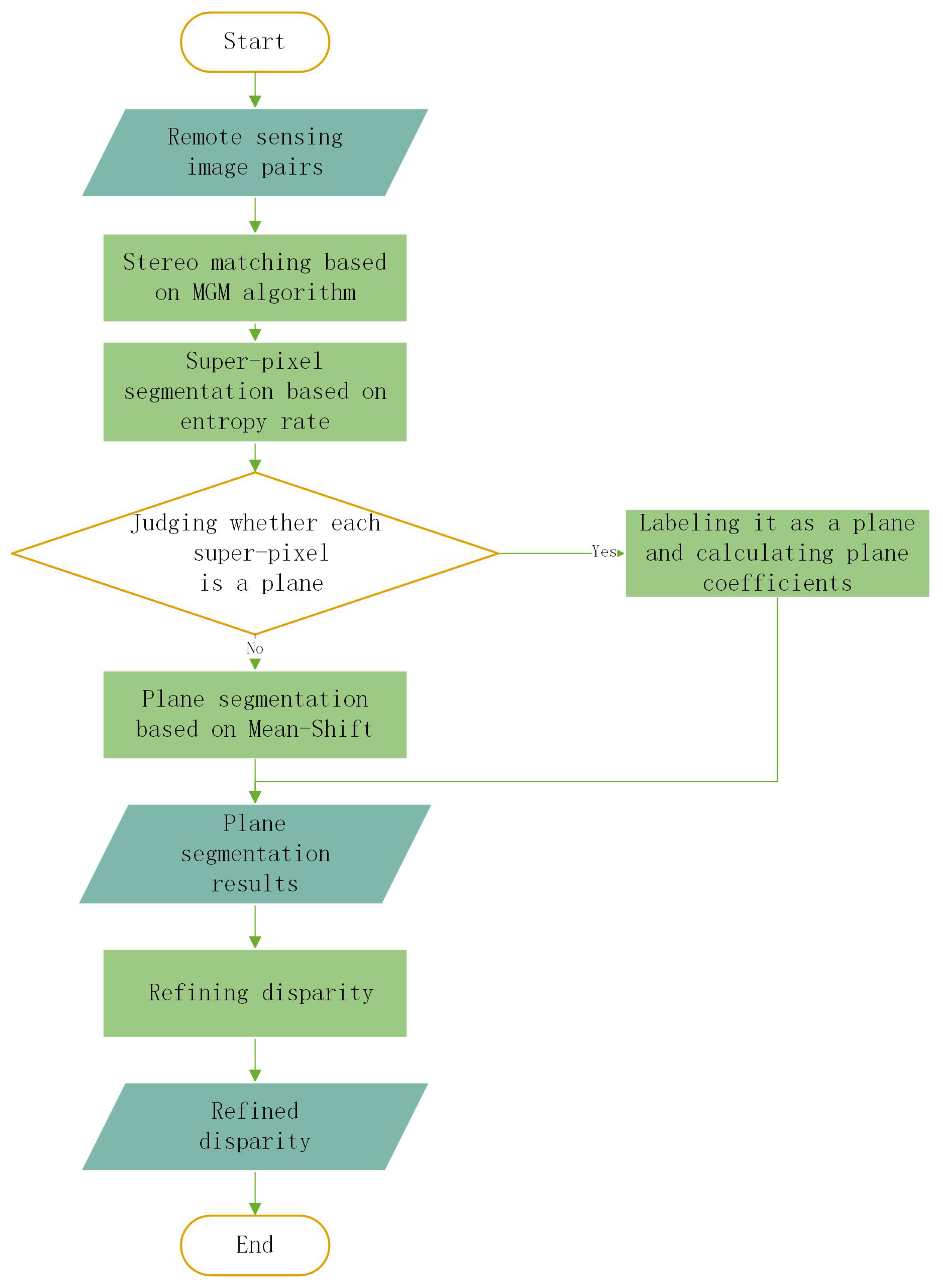
Our method mainly includes four steps as follows: (1) calculating the disparity based on the More Global Matching (MGM) algorithm [18], (2) segmenting super-pixels based on the entropy rate algorithm [48], (3) segmenting planes based on mean-shift-based plane segmentation, and (4) correcting the disparity based on planes. The specific process is shown in Figure 1.
Because sometimes the illumination difference between the left and right images was large, the linear contrast stretching method was used. The gray intervals of both left and right images were expanded to [0, 1] to reduce the difference between the brightness of the two images.
Semi-global matching (SGM) is the most used stereo matching algorithm [19,20,21,22]. The objects in the Worldview-1 images used in this paper have a large deformation. Through the effect evaluation (see Section 3.1.2 for details), we found that the MGM algorithm worked better than SGM in such images, so the MGM stereo matching algorithm was selected for this study. Combined with super-pixel segmentation, plane segmentation can utilize color and texture information in an image while many super-pixel blobs are themselves planes, which can improve the efficiency of the segmentation algorithm. We chose a method based on the entropy rate that obtained more accurate super-pixel edges. Therefore, our method first judges planes for super-pixels, and plane segmentation is performed on non-planar super-pixels. After estimating all plane equations, the outliers were removed for each plane according to the distances to the plane, and the missed matching pixels were filled.
2.2. Plane Segmentation Based on Mean-Shift and Energy Minimization
Because our plane segmentation is combined with super-pixel segmentation, the requirements of the plane segmentation algorithm in this paper are different from other algorithms, and there are few planes involved in one segmentation. The main requirements of our algorithm are as follows. (1) It is required to have a strong anti-noise ability because there is often a certain amount of noise in the stereo matching results. (2) It should be able to approximate the curved surface by a combination of planes. (3) The speed should not be slow. Because it is combined with other algorithms, a slow speed will cause low algorithm efficiency.
Traditional fast algorithms are implemented either by region growing or square supervoxel clustering. The region growing has a poor noise resistance ability, and square supervoxel clustering is not suitable for approximating the curved surface. Our algorithm is implemented in two steps. The first step is a fast initial segmentation based on the mean-shift algorithm, and the second step is a precise segmentation based on energy minimization.
2.2.1. Fast Initial Segmentation Based on an Adjusted Mean-Shift
- A.
- The original Mean-Shift algorithm
Mean-shift is a non-parametric clustering algorithm based on density. The steps for forming one category of mean-shift are given below.
- 1.
- Point C in the sample space is selected as the center of the sphere. A high-dimensional sphere is formed with radius r, and all the points in the sphere are found. The high dimensional sphere radius r is the main parameter of mean-shift algorithm and it is determined by tests usually.
- 2.
- The mean value of all points is used as the new center of the sphere. If the difference between the new sphere center and the previous sphere center is less than a threshold T, then the algorithm exits this step and proceeds to Step 3; otherwise, it returns to Step 1. In this paper threshold T is 0.01.
- 3.
- When the algorithm exits the above two steps, the points passed by the sphere all belong to the same category.
These three steps obtain samples of one category. After removing these samples from the total samples, Steps 1–3 are executed on the remaining samples, and all the categories will then be gradually obtained.
- B.
- Plane segmentation algorithm based on mean-shift
The mean-shift clustering algorithm is highly suitable for plane segmentation because of the fast speed and because the number of categories do not need to be defined in advance. The key steps of plane segmentation are the same as the original algorithm, but the following adjustments are required:
- 1.
- Plane fitting in clustering
The original mean-shift clustering method can be regarded as the moving process of the hypersphere. In plane segmentation, clustering is a moving process of the circle. According to the original deduction, the fastest moving direction is obtained by the mean of the samples in the circle. The first difference between our method and the original algorithm is that, before calculating the sample mean, it must be determined whether the current circle is a plane. If it is a plane, then the circle continues moving.
- 2.
- Using the mean value of newly added points as the center of the next circle
Mean-shift clustering assumes that the point with the highest density is the cluster center. However, data points are approximately uniformly distributed in plane segmentation, so there are many points with the same density. The original mean-shift algorithm will stop prematurely at one of them. We adjusted the original algorithm from calculating the mean value of all points within the circle to calculating the mean value of the newly added points as the new center. In this way, the algorithm keeps moving until it meets a non-planar point (Figure 2). In one time clustering of circle movements, although the entire plane may not be completely covered, the coverage area expands substantially in comparison with the original algorithm, which significantly improves algorithm efficiency. A new sample point is randomly picked from the uncovered dataset as the new center of the circle, and it starts moving again. When the new center is taken from the remaining points in the incompletely covered plane, a new cluster will be formed and merged with the obtained co-planar category so that the entire plane can be covered.
A series of movements of the circle in the algorithm is shown in Figure 2, where the red circle is the cluster center of each time. If the mean value of all the points in the circle is calculated as the new center according to the original algorithm, then the movement of the circle will soon stop. Because it only calculates the mean value of newly added points, the circle will keep moving and clustering until it meets a non-planar point, as shown in Figure 2a. Although there are remaining points in the plane, they will be selected later and then fitted, as shown in Figure 2b. After fitting, they will merge with the last category.
- 3.
- Pre-processing and post-processing
Pre-processing removes the points with large curvatures [33]. Points with large curvatures are generally not a plane point. Therefore, the curvature of all the points is initially calculated and the points with large curvatures are removed to avoid their interference with plane fitting. They are then stored in the non-planar point set.
Post-processing deals with non-planar points. For each point category, label numbers around the point are extracted. After calculating errors of the point to all neighboring category planes according to Equation (3), this point will be classified into the category with the smallest error.
Compared with the original algorithm, two temporary point sets are used. One is the visited plane point set, which is called the previous point set. The other is a new point set calculated according to the current mean value, called the current point set. When the mean shifts, if the current point set is a plane and belongs to the same plane as the previous point set, then the current point set will be merged into the previous point set. Centered on the mean of the current point set, the new points in the circle are extracted as the new current point set. Otherwise, the previous point set is labeled as a new category. The initial plane segmentation algorithm is described in detail in Algorithm 1.
| Algorithm 1: Initial plane segmentation. |
 |
 |
For plane fitting, RANSAC is the best, but the running time is too long. We use double thresholds of the plane error and density to judge whether a point set is a plane. In the current point set, the points whose errors are less than the plane error threshold are regarded as the plane point. If the ratio of plane points is larger than the density threshold, then the current point set will be judged to be a plane. The plane equation is estimated from plane points based on the least squares method.
There is only one traverse of all the pixels in the non-planar point extraction part of this algorithm. In the process of cluster forming, each new category is judged in terms of whether it will be merged with the old categories, which is implemented using a double loop of . Therefore, the overall computational complexity is less than .
2.2.2. Precise Segmentation Based on Energy Minimization
After the initial segmentation, there are several inaccurate edges or non-merged planes, which must be improved by precise segmentation implemented by energy minimization. The definition of the energy function is the same as in the literature [31]. The energy function is given in Equation (1).
Here, l denotes the pixel category label and is the label of the pixel p, is the label category set, is the plane corresponding to the category, N represents the pixel neighborhood, is the constant coefficient corresponding to the label cost, is the number of labels, and is the inliers range threshold.
The data cost is the sum of the normalized error (i.e., distance) from each point p to the plane . The smoothing cost penalizes the inconsistency of the labels in the neighborhood, and the Potts model (Equation (4)) is chosen here. The label cost punishes redundant planes, and its goal is to alleviate the over-segmentation problem. The alpha-expansion algorithm is used as the energy function minimization method [39], which is implemented using a loop of . Therefore, the overall computational complexity is less than .
2.3. Disparity Plane Fitting and Disparity Refinement
The distance in Equation (3) is a 3D plane distance. In the disparity calculation, the disparity changes only by the x coordinate. Assuming that is the corresponding point in the left and right images, then, in the images after epipolar rectification, , and the disparity is calculated by Equation (5).
Equation (5) is converted to , which is still a plane equation. Here, corresponds to in the 3D space, but the coefficient of z is −1. The plane coefficients are , which can be calculated by Equation (3). After the disparity plane is fitted, outlier removal and missed matching area filling should be performed. Outlier removal calculates the error of each pixel in the plane according to Equation (5), that is, the distance to the plane. When the error is larger than the inlier point threshold, it belongs to the outlier, and its disparity will be corrected according to the plane equation. Before filling the disparity, category labels should be assigned to the missing matching pixels, in which there are two cases. In the first case, a super-pixel is a plane and the missing matching pixels in it are filled according to the plane equation. In the second case, a super pixel includes multiple planes and each missed pixel in it belongs to the closest plane. The specific implementation is to cyclically perform a single pixel dilating operation on each plane until there is no missing matching pixel in the super pixel. The pixels first touched by a plane belong to this plane and the label is filled in the label image. It would not be modified later. After all the missed pixels in the super pixel are labeled, their coordinates and disparities are calculated according to Equation (5).
Compared with interpolation methods [25,26,27], the proposed algorithm first performs plane segmentation and fitting and corrects the disparity according to plane model, which will obtain more accurately disparity refinement results.
Compared with the method using plane fitting [28], they have just performed a single plane fitting to each super-pixel, which is the single plane fitting based method. Our algorithm first performs single-plane fitting on plane super-pixels also, and then performs plane segmentation on non-plane super-pixels. More planes are fitted than the single plane fitting based method. Since our plane segmentation algorithm has certain anti-noise performance, and considering the time complexity, we did not use the RANSAC. Compared with this type of method, the proposed method does not consider the smoothness with neighboring pixels when filling the disparity. Developing disparity smoothing suitable for remote sensing images is the future work on algorithm improvement.
3. Results
3.1. Edge Matching Rate and Edge Matching Map
Stereo matching of ordinary images is generally tested on the Middlebury stereo matching test platform. Stereo matching results of remote sensing images are evaluated by an elevation map. Compared with common images, the matching difficulty of different remote sensing images varies significantly. Remote sensing images with different matching difficulties cannot be compared to each other by an elevation map. In some cases, elevation maps of the matching images cannot be obtained. To analyze stereo matching results without the ground truth, the EMR and EMM were proposed. These are used as measures of the matching effect.The Canny operator with default threshold ([0.0313, 0.0781]) is used to obtain the edge maps. The EMR is the ratio of edge points to matching edge points in another image, and it is calculated by Equation (6).
Here, is the total number of edge points in the left image, and is the number of edge points in the right image after adding disparity to the edge points of the left image. Because the edges and textures contain most of the image information, the EMR can represent the matching accuracy to a certain extent. Corresponding to the EMR, the EMM is a color image, where the first channel is the edge of the right image, and the second channel is the result of adding disparity to the edge of the left image. In an EMM, the yellow edge pixels refer to the correct matches. If there are many red and green edges in it, it indicates that the matching accuracy is poor. The matching effect is clear from the EMM.
3.1.1. Test on the Middlebury Dataset
The SGM, MGM, and Graphcut (GC) algorithms were used to match the Middlebury images. The effect was evaluated by the EMR and EMM. The absolute difference between the disparity and the ground truth was defined as the matching error. The pixels with matching errors less than the threshold (the threshold was set to 1) were regarded as correctly matched pixels. The rate of matched pixels to the total pixels was the matching accuracy rate(MAR), which was used as the measurement. The EMMs of some images are shown in Figure 3. The EMR and EMM results are exhibited in Table 1.
As shown in Table 1, the average EMR of the SGM was as high as 81.6%. The EMRs of MGM and GC were less than 45%. From the EMMs, SGM also had the best matching effect. The average EMR of MGM was lower than that of GC. However, the EMM shows that there were more complete and correct matching areas in the MGM results. Most of the matching edges were correct matches, but there were more missing matches, so the EMR was lower than GC. In the EMMs of GC, most of the edges were mismatched, and most of the coincided edges were not correct. Although the EMR of GC was higher than MGM, the matching effect was poor. Therefore, the matching performance of MGM was better than that of GC. Through EMR and EMM, it can be judged that the matching performance order of the three algorithms is SGM, MGM, and GC, and the evaluation results of MAR is the same.
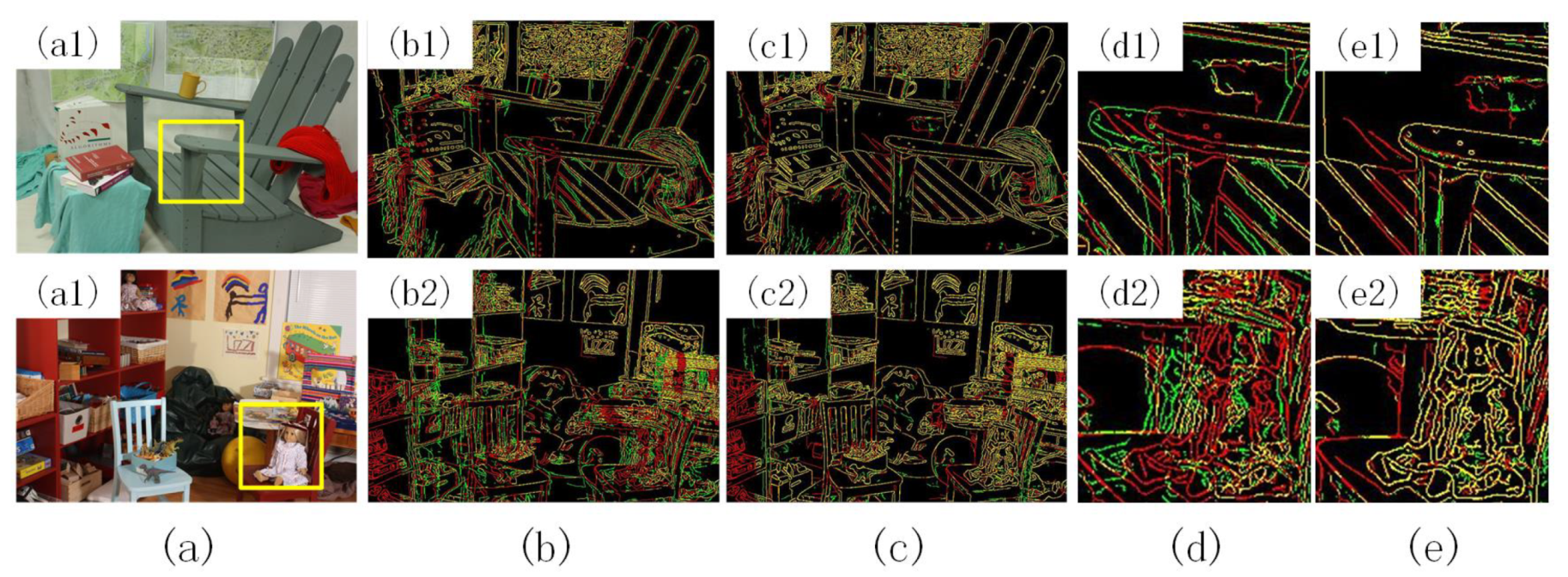
Through the EMMs, we found some wrong matches in the ground truth images, as shown in Figure 4. There were also some errors in other ground truth disparity images in this dataset. These images were found by comparing the EMR of the SGM with that of the ground truth and observing the EMM. Therefore, the EMR of SGM was higher than that of ground truth, which is a correct evaluation.
From EMM we found that most of the matching results of MAR over 10% were relatively fine, and there were many correct matching edges in them. A small number of matching results with MAR less than 10% are tolerable. From Table 1, when MAR results are more than 50% EMR are usually above 10%, and many correct matching edges can be found by observing EMM. It can be concluded that the EMR threshold for good matching should be 50%.
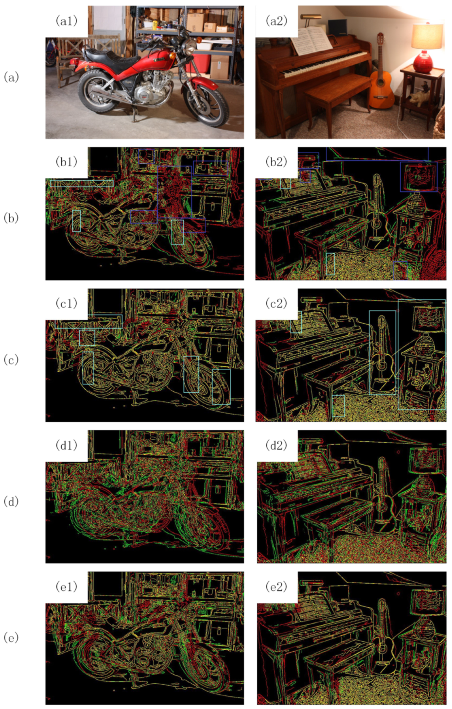
However, the matching results with EMR above 50% did not show the trend of MAR strict increasing or decreasing with EMR, which may be caused by two reasons. First, there are some errors in the Ground truth results, and these errors will cause some MAR deviations. Second, EMR has a little ambiguity because the matched edges cannot be completely guaranteed to be the correct matched edges. A matching effect with 51% EMR may be as same as that with 53% EMR. But for the same image, when the EMR difference is obvious, the higher the EMR, the better the matching effect. This can be proved by comparing the EMR and EMM images of Motorcycle and Piano images in Figure 3. Due to some errors in Ground truth disparity maps, we cannot use MAR to explain the EMR trend, which can only be illustrated by EMM.
The EMR values of MGM, Ground truth and SGM are at 50%, 60% and 80% level respectively, and from their EMM images it can be found that the matching effects are consistent with EMR trend. In Figure 3, we used rectangular boxes to represent the regions in which the results of MGM, SGM were significantly better or worse than ground truth. The regions in dark blue boxes were obviously worse, the light blue regions were obviously better. To avoid visual confusion, there was no box on the ground truth images. First, (b) MGM and (e) ground truth in Figure 3 were compared. In Motorcycle EMMs, there were five regions in which MGM was worse than ground truth, and there were three regions in which MGM was better than the ground truth. In the Piano EMMs, there were six worse regions and two better regions. In short, in the MGM results, there were more worse regions and they were larger than better regions. Then (c) SGM and (e) ground truth in Figure 3 were compared. Since SGM’s EMR was nearly 20% higher than Ground truth, its advantages were more obvious. The two images included respectively five and four regions in which SGM was significantly better than ground truth, and there were almost no significantly worse region. This trend also exists in other images with large EMR greater than 50%. Therefore, when EMR is greater than 50% EMR can reflect the matching effect to a certain extent.
From the analysis of the matching edge effect, the main factor affecting the accuracy of EMR is the incorrect matching edge, which are caused by that the wrong disparity makes the edges in one image coincide with incorrect edges in another image. As shown in the two EMM images of GC in Figure 3c. This causes that EMR below 50% cannot be used alone to measure the matching effect.
Combining the results of EMR, EMM, and MAR shows that, when the EMR is more than 50%, the higher the EMR is, the better the matching performance is. When the EMR is below 50%, it needs to judge the effect by observing the completeness of the matching edge in the EMM.
3.1.2. Test on Remote Sensing Images
We verified the reliability of the EMR and EMM using remote sensing images. Some of the images and EMMs are shown in Figure 5. The EMR and elevation error of these block images are given in Table 2.
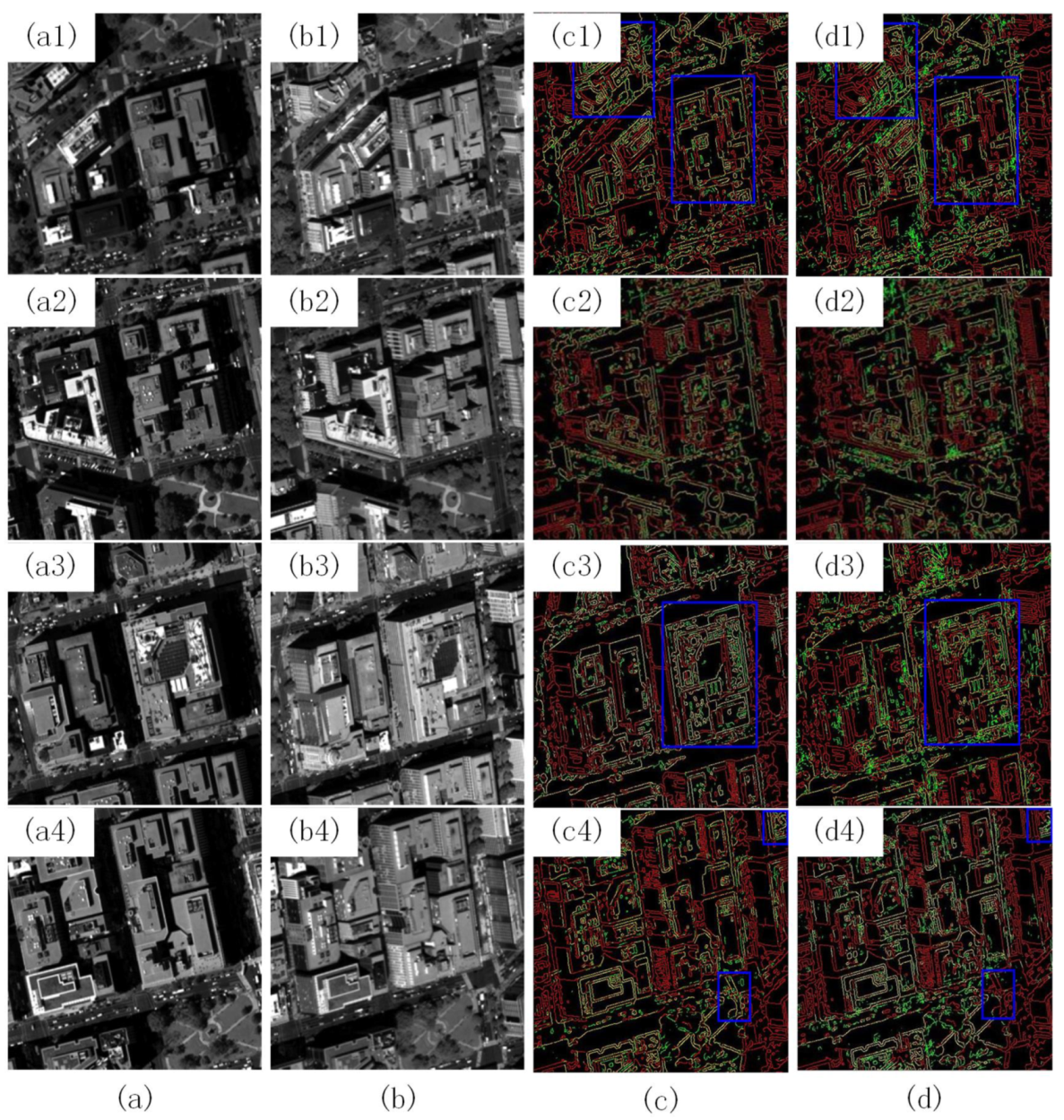
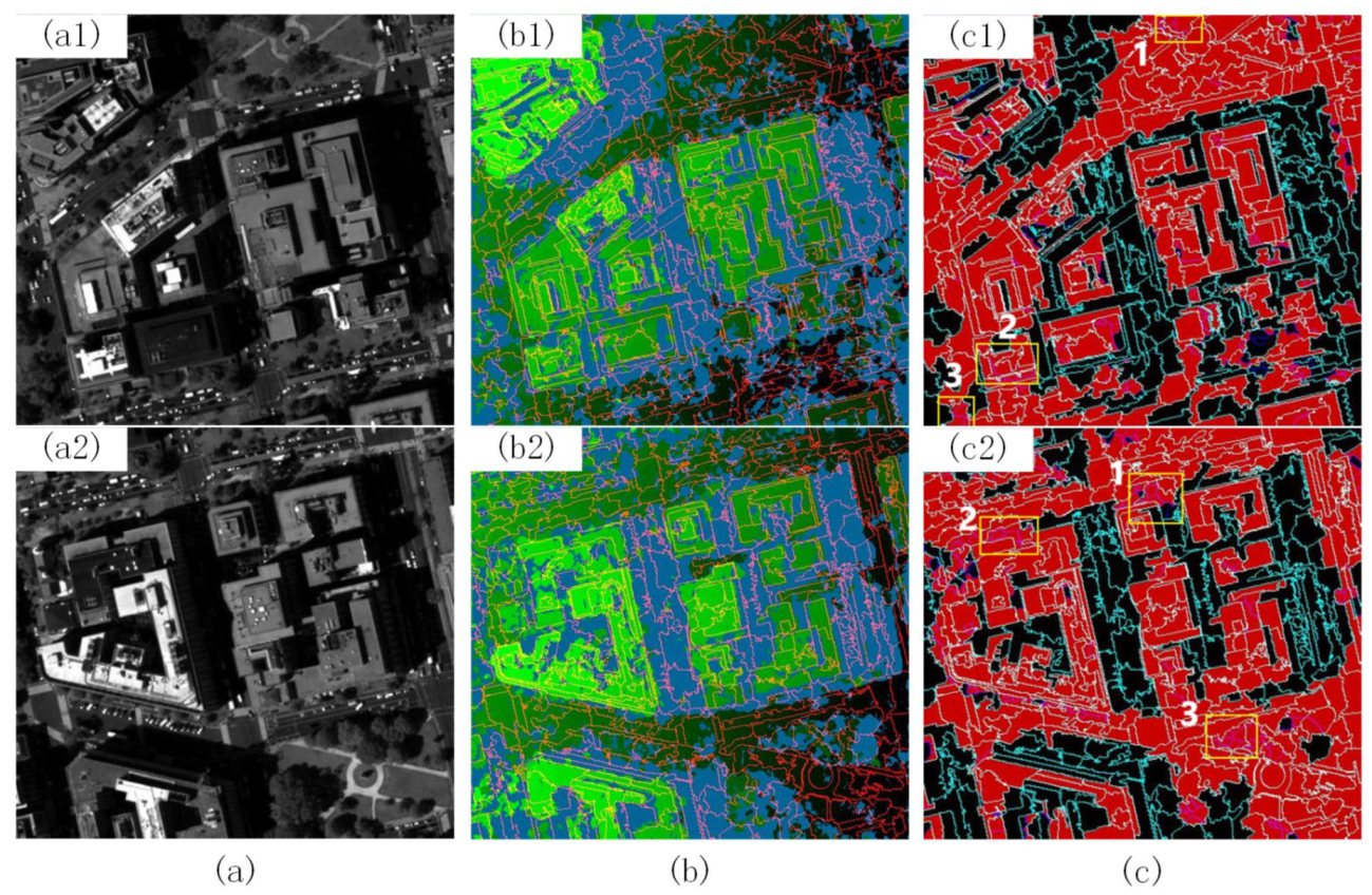
From the remote sensing image example, the difference between the left image and the right image was large. For example, only the roofs of the buildings can be seen in the left image in the first row of Figure 5. The side walls of the buildings can be seen in the right image, where there is a large deformation between image pairs due to different positions. If the building is taller, then the deformation will be larger, and matching is much more difficult than in ordinary images. In remote sensing images, the matching effect of the GC algorithm was very poor, so we used the MGM and SGM algorithms for comparison.
From the EMR, the MGM was like SGM, and both were about 45%. In the EMMs, MGM had good integrity and few errors, especially for the roof part with a rich texture. However, MGM had a considerable part of missing matches. Most of these missing matches were in the shadow parts of low-texture and low-gray-scale areas, in which matching is very difficult. The EMR of SGM was not low, and the matching edges were not as complete as MGM. Moreover, there were many wrong matches in the EMM of SGM. For the stereo matching algorithms, the matching results at the locations of edges and rich textures will affect the matching of neighbor pixels with consistent gray values, so a wrongly matched edge may mean a small, incorrectly matching area. Therefore, the matching errors of SGM will be larger than MGM. The elevation error in Table 2 supports this conclusion. The average EMR and elevation error of all block images are shown in Table 3. The conclusions reached by the EMM analysis were correct. In summary, in this kind of remote sensing image with large deformation, MGM is better than SGM.
3.1.3. Summary
According to the analysis of the above results, edge and texture locations with rich edge points contain the main information of an image, so edge matching can determine the matching effect of the entire image. According to Section 3.1.1 and Section 3.1.2, the matching effect through EMR and EMM in the absence of ground truth disparity can be analyzed. When the EMR is more than 50%, it can be used to evaluate the matching effect. The higher the EMR is, the more accurate the matching result is. When the EMR is less than 50%, some matching edges may coincide by accident and match the wrong edge pixels. In this situation, the matching effect can be judged by analyzing the matching completeness of areas and the number of wrong matches in EMM. Both EMR and EMM are suitable in either ordinary or remote sensing images. Furthermore, they can find errors in ground truth disparity.
Since the coincident edge is not directly equal to the correct match, both EMR and EMM also have shortcomings. Compared with measures, such as MAR and mean absolute error, the EMR is something fuzzy, and thus it cannot measure the small differences between matching results, and it is not a precise evaluation measurement. Nevertheless, EMR and EMM are still easy-to-use, widely applicable, intuitive, and effective measure and analysis tools.
3.2. Plane Segmentation
Our plane segmentation algorithm was evaluated using a plane segmentation dataset, which was then compared with the Plane Extraction Using Agglomerative Hierarchical Clustering (PEAC) algorithm [49].
3.2.1. Evaluation Dataset and Measures
The plane segmentation dataset SegComp was chosen as an evaluation dataset [39]. Thirty relatively complex point cloud images were selected from the dataset_test part. These included most of the planes and several curved surfaces. In addition to SegComp, we created a small dataset including three point clouds, that is, a semi-octahedron (half of an octahedron, which was used for algorithm demonstration and anti-noise experiments), Gaussian curved surfaces, and decreasing sine curved surfaces. The semi-octahedron was generated by defining the vertex of each face. Equations of the Gaussian curved surface and the decreasing sine curved surface are given in Equations (7) and (8), as follows:
where the values of h and r were 150 and 90, respectively, and x and y ranged from −r to r (in Equation (7)). The value of h was 50, and x and y ranged from −8 to 8, with a 0.1 interval (in Equation (8)).
For a plane segmentation algorithm, segmentation results are usually evaluated through measures such as the correct segmentation rate and direction deviation. Because our plane segmentation algorithm was used for disparity filling, we used fitting error as the evaluation measure. First, the planes were fitted based on plane segmentation algorithm, and the equation coefficients of each plane were calculated. The average distance from the points to its plane was then calculated according to Equation (3) as the error to evaluate the algorithms.
3.2.2. Plane Fitting Effect
Our plane segmentation algorithm mainly included two parameters. After estimating the plane equation of the point set, the plane error threshold was used to judge whether a single data point was a plane point, and the density threshold was used to judge whether the point set was a plane. For plane images, Gaussian noise with a mean value of 0, a variance of 0.01, and an amplitude scale factor of 0.03 was added. No noise was added in the curved surface images. The correlation between the two thresholds and fitting error was calculated and the two values that minimized the fitting error were selected as thresholds. The error threshold was 0.3, and the density threshold was 0.8. The default parameters were used for the PEAC algorithm. The plane segmentation results of some examples are shown in Figure 6.
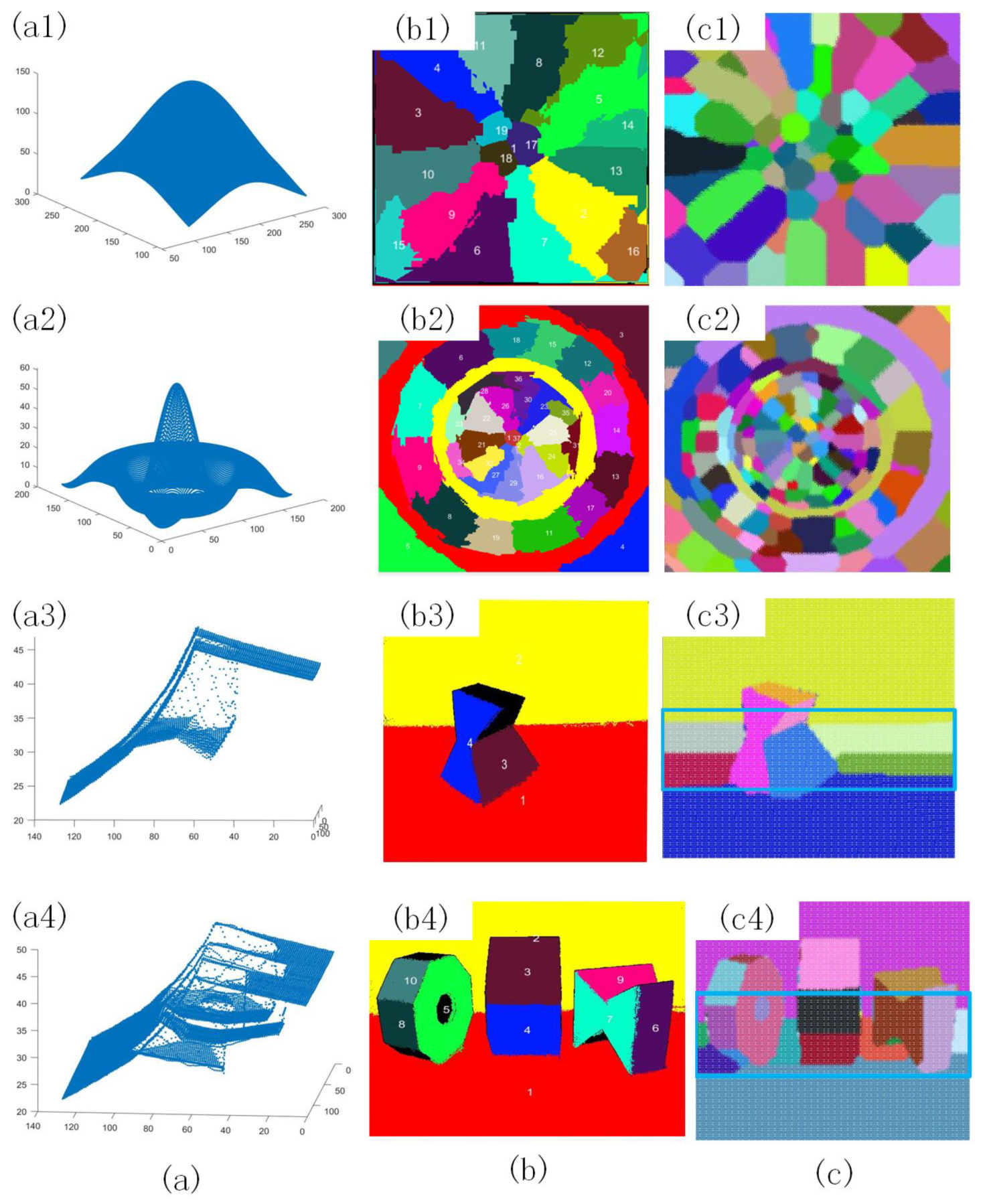
Both our algorithm and the PEAC algorithm could accurately segment the plane, but they made some mistakes at edge locations, as shown in Figure 6. For the curved surface, our algorithm fitted more finely than the PEAC algorithm. For the two SegComp examples (Rows 3 and 4), the lower half of the background was a curved surface (a), which was segmented into a plane using the PEAC algorithm (the red area in (b)). Our algorithm segmented the surface into different planes, which were smooth (Row 3 of (c)). According to the labeled images of the SegComp images, the results of PEAC segmentation were correct. To reduce the fitting error, a curve face should be approximated by planes. There were many objects in Row 4 of (a), so our algorithm segmented it into more planes than Row 3. From the area in the box, its width was consistent with the same region in the image of the third row. The curved surfaces of the segmented planes of our algorithm were smoother than the PEAC. We calculated the plane fitting errors of different algorithms, which are shown in Table 4. The error of our algorithm was lower than that of the PEAC algorithm. The reason for this may be that internal parameters of PEAC were adjusted more suitable for label images of the SegComp dataset.
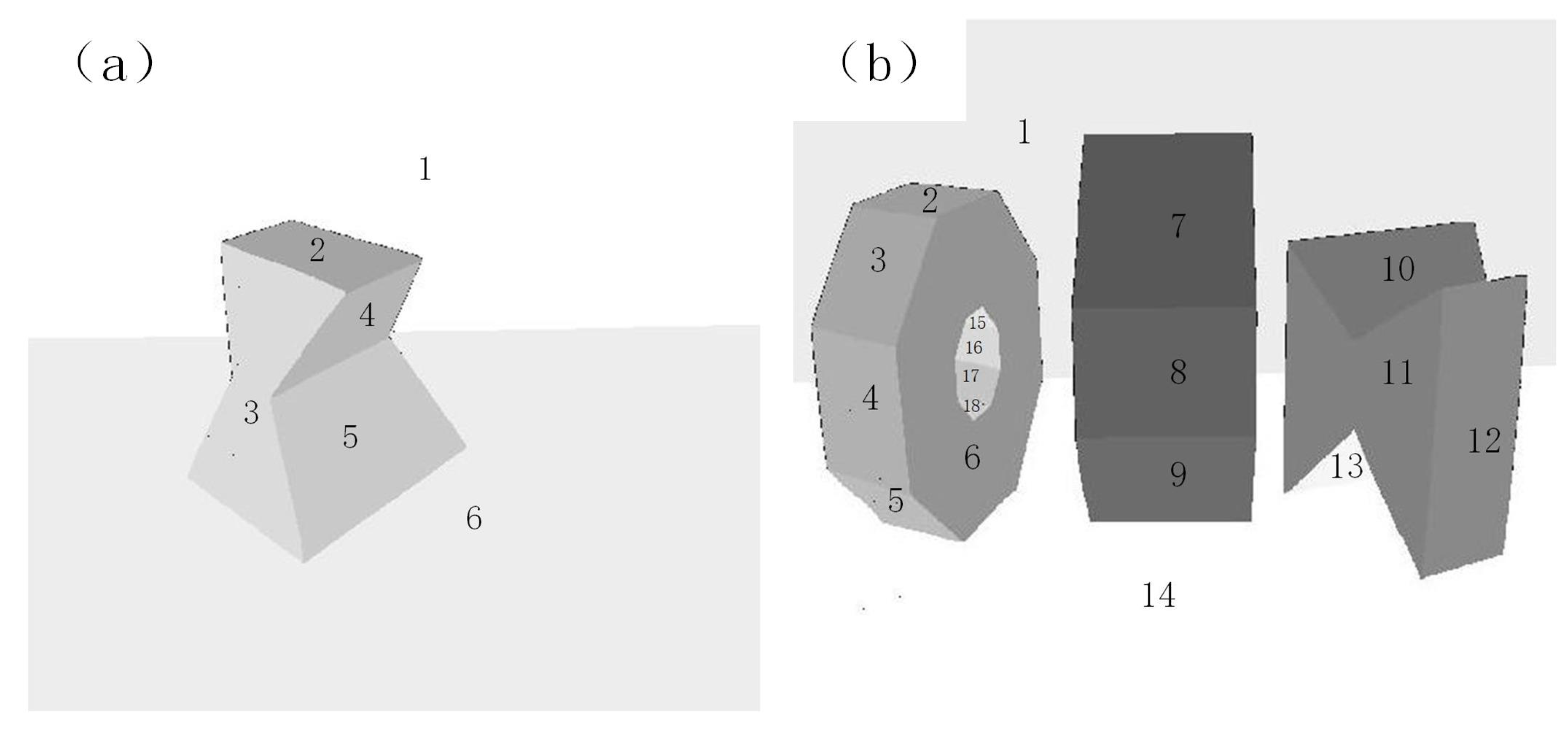
According to ground truth images in Figure 7, there are 6 planes in Figure 6(a3) and 20 planes in Figure 6(a4). The estimated plane numbers shew in Table 4. The PEAC algorithm estimated 4 and 10 planes respectively, which was under-segmented. Our algorithm estimated 30 planes in total. For Figure 6(a3,a4), 5 planes and 15 planes were correctly segmented respectively. For Figure 6(a4) plane 15–18 were segmented into one plane. Although the results of our algorithm were over-segmented to a certain degree, the number of correct planes was more than that of PEAC, which proved the effectiveness of our algorithm on the other hand.
3.2.3. Anti-Noise Performance Analysis
To verify the anti-noise performance of our algorithm, ‘salt‘ and Gaussian noise were added into the plane images (semi-octahedron and SegComp dataset). The density of the ‘salt‘ noise ranged from 0.05 to 1, with a 0.05 interval, and the amplitude scale factor ranged from 0.001 to 0.08. The mean value of Gaussian noise was 0. Its variance ranged from 0.01 to 0.15, with a 0.02 interval, and the amplitude scale factor ranged from 0.005 to 0.07. The noise amplitude was the result of the amplitude scale factor multiplied by the maximum height of the point cloud. For example, the maximum height of the SegComp dataset was 4600. When the amplitude scale factor was 0.01, the maximum amplitude of the noise was 46. Therefore, the amplitude scale factor represented the intensity of the noise. For zero-mean Gaussian noise, the greater the variance was, the greater the noise density was. Thus, the variance represented the noise density. After adding noise, the point clouds were segmented, and the maximum noise amplitude and density parameters to obtain correct segmentation were recorded and are shown in Figure 8. Correct segmentation means that the results after adding noise were the same as those before adding noise.
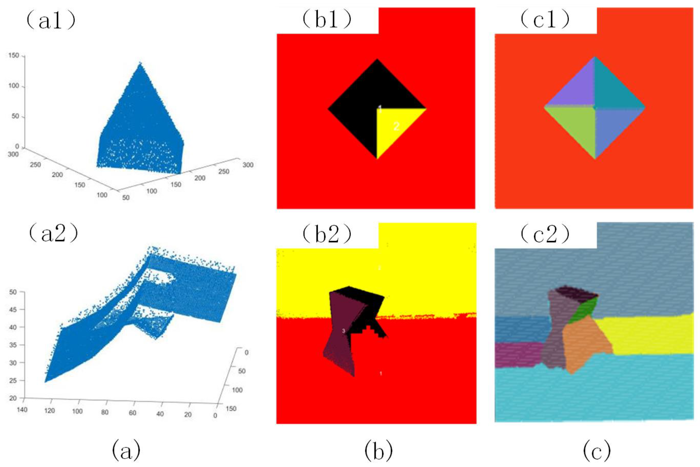
The horizontal axis represents the noise density, and the vertical axis represents the noise intensity. The curves of our algorithm were all above the PEAC algorithm (Figure 8a,b), which indicates that our algorithm could withstand a higher noise intensity than the PEAC algorithm at the same density. The ‘salt‘ noise with a density of 0.2 and an amplitude scale factor of 0.05 was added to plane clouds, and the fitting effect of our algorithm and the PEAC algorithm is shown in Figure 9. Our algorithm could segment the planes correctly, while the PEAC algorithm result had partial errors. Based on the experimental results in Section 3.2.1 and Section 3.2.2, the proposed algorithm accurately achieved plane segmentation and surface approximation while possessing some noise-resistance ability. The plane segmentation effects in disparity refinement are described in Section 3.3.
3.3. Disparity Refinement
3.3.1. Plane Segmentation Result
The MGM algorithm was used to obtain the disparity map on the block images obtained in Section 3.1.2. First, the left image was segmented into super-pixels. Combining super-pixel results with the disparity map, planes were segmented according to the process described in Section 2.1.
The circle radius of the mean-shift was 5. The plane error threshold and density threshold were respectively 1.6 and 0.5, and the inlier point threshold was 6. The threshold determination process is as follows:
We selected five images for determining the thresholds. First the error and density thresholds were determined. The initial error threshold was 0.8 and the density threshold is 0.7. Then plane segmentation was performed and plane segmentation images like Figure 10c were generated. Then we checked whether plane super-pixels were all estimated as planes. If there were under-estimated plane super-pixels we increased the error threshold or reduced the density threshold till the estimated number of plane super-pixels was closest to the true number. In our experimental images, there were 1020 plane super-pixels in total. Table 5 listed the plane super-pixel numbers estimated by different threshold combinations. The closest total plane number 1014 was obtained when the error threshold value was 1.6 and the density threshold was 0.5. When the thresholds were 1.7 and 0.5, the estimated number of planes was 1031, which means that some non-planes were estimated as planes. Therefore the error threshold and the density threshold were selected 1.7 and 0.5.
After determining the error and density threshold, the bandwidth threshold is estimated by calculating the average error of the plane fitting (Plane fitting results were like images in Figure 11b). Since the plane segmentation was performed on super-pixels, the bandwidth range was as small as [3–7] and it was easy to determine. Table 6 showed the determination of bandwidth and inlier point threshold. In Table 6, the first column was the bandwidth, and the second column was the plane fitting error. The bandwidth 5 corresponded to the smallest fitting error, so the bandwidth threshold was chosen to be 5. Finally the inlier point threshold was estimated by calculating the height error after the disparity refinement. After the above three thresholds were determined, the disparity refinement can be performed, then the inlier point threshold can be obtained by calculating the elevation error. When the threshold was 6, the elevation error was the smallest, so 6 was selected as the interior point error threshold.
The plane segmentation results of two pairs of images are shown in Figure 10. Figure 10b are disparity maps, where the first channel is the original super-pixel segmentation result, and the disparity was used as the second channel. The first channel of the plane segmentation image in Figure 10c was a binary plane image in which the plane pixel gray value was 255 and the other pixel value was 0. The second channel was the original super-pixel boundary image. The super-pixel boundary after plane segmentation was the third channel. In such an image, the pure red super-pixel indicated that the whole blob was a plane. If a super-pixel contained a blue or purple boundary, then it indicated that it was segmented into several planes further.
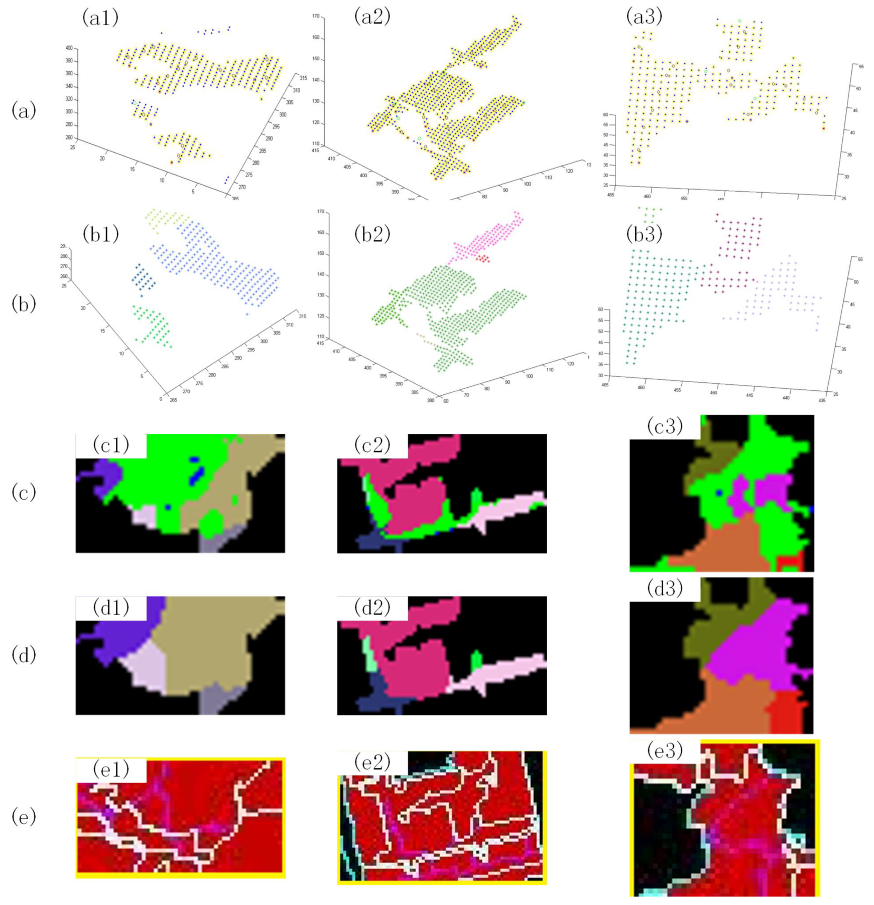
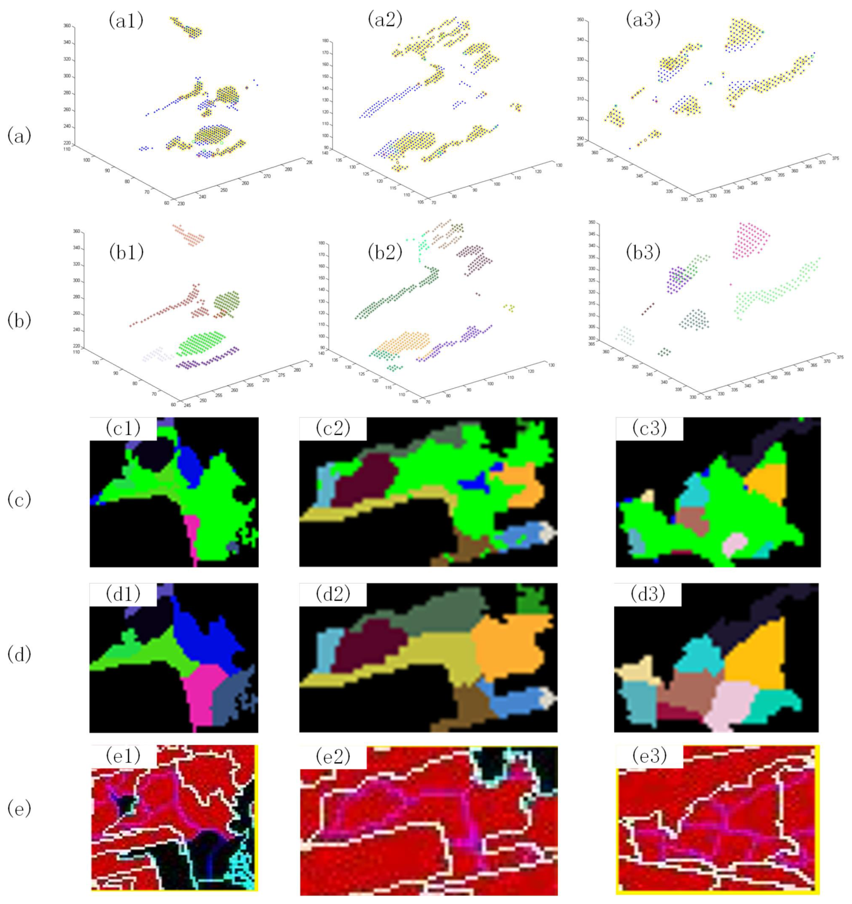
Figure 11 and Figure 12 have similar content. Among them, (a) includes 3D figures of the super-pixel points to be segmented. Its x, y, and z axes correspond to the x-coordinate and y-coordinate of the left image and the x-coordinate of the right image, respectively. The x-coordinate of the right image increased with the growth of the x-coordinate in the left image, so the plane was always upward. In these figures, the small red circles are the mean-shift centers. The 3D figure of plane fitting results is shown in (b). Different colors represent different segmented planes, and the colors were randomly generated. Here, (c) includes the labeling figures of plane segmentation, in which the missed matching pixels are green. There were a few non-planar points that were unsegmented, shown in blue color. The remaining colors that were randomly generated represent the labels of the plane segmentation. The colors in (c) are different than the colors in (b). In addition, (d) contains the results of expanding the segmentation regions, while the missed matching and non-planar points are filled in (c). The colors of (c) and (d) correspond to each other because the same plane is shown in the same color. The boundary images of the plane segmentation are in (e), and these were obtained from the rectangles in Figure 10c. As can be seen in Figure 11b and Figure 12b, the missed matching pixels divide the disparity map into many fragment regions that were fitted and segmented into planes. The planes expanded outward to form relatively uniform blobs, covering the missed matching area (Figure 11d and Figure 12d).
There are many planes in urban remote sensing images, so many planes were fitted in these images. The plane segmentation results of several super-pixels are shown in Figure 11 and Figure 12. The three columns in Figure 11 correspond to the three super-pixels in the labeled rectangles in the first row of images in Figure 10c, and Figure 12 corresponds to the second row of images in Figure 10c.
3.3.2. Disparity Refinement and Three-Dimensional Reconstruction
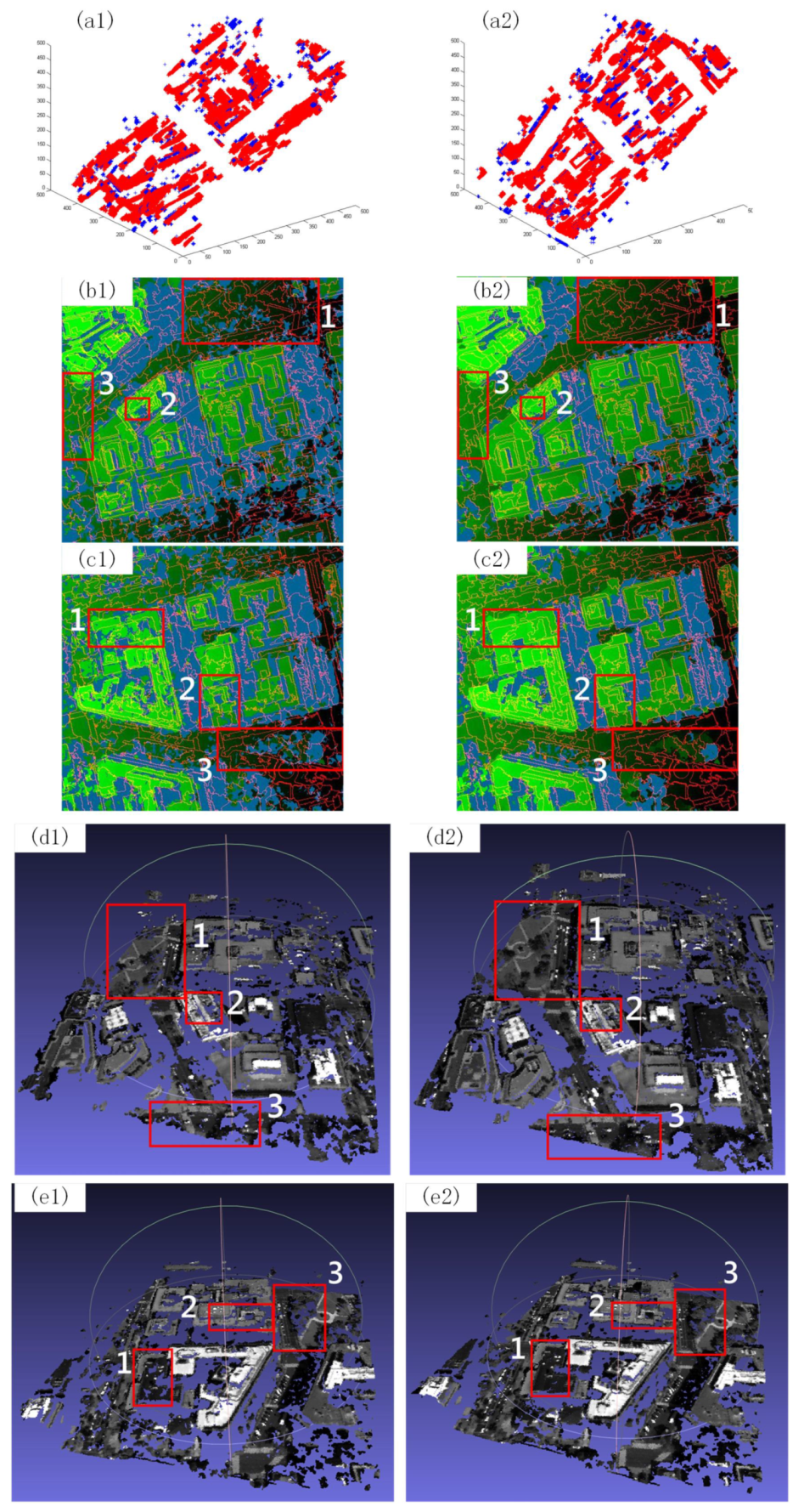
In Figure 13, Example 1 and Example 2 correspond to the first- and second-row images in Figure 10. The outlier removal effect is shown in Figure 13a. Here, the inliers are red points, and the outliers are blue points. Figure 13b,c are disparity maps that have the same channels as those in Figure 10b. The third channel is the missed matching pixels, so the brighter the green color is, the larger the disparity is. The blue area is the missed matching pixels. The 3D point cloud images before and after filling the disparity are shown in Figure 13d,e. As a supplement to Figure 13. Figure 14 is correspond to the boxes in Figure 13b,c. Figure 15 is correspond to the boxes in Figure 13d,e.
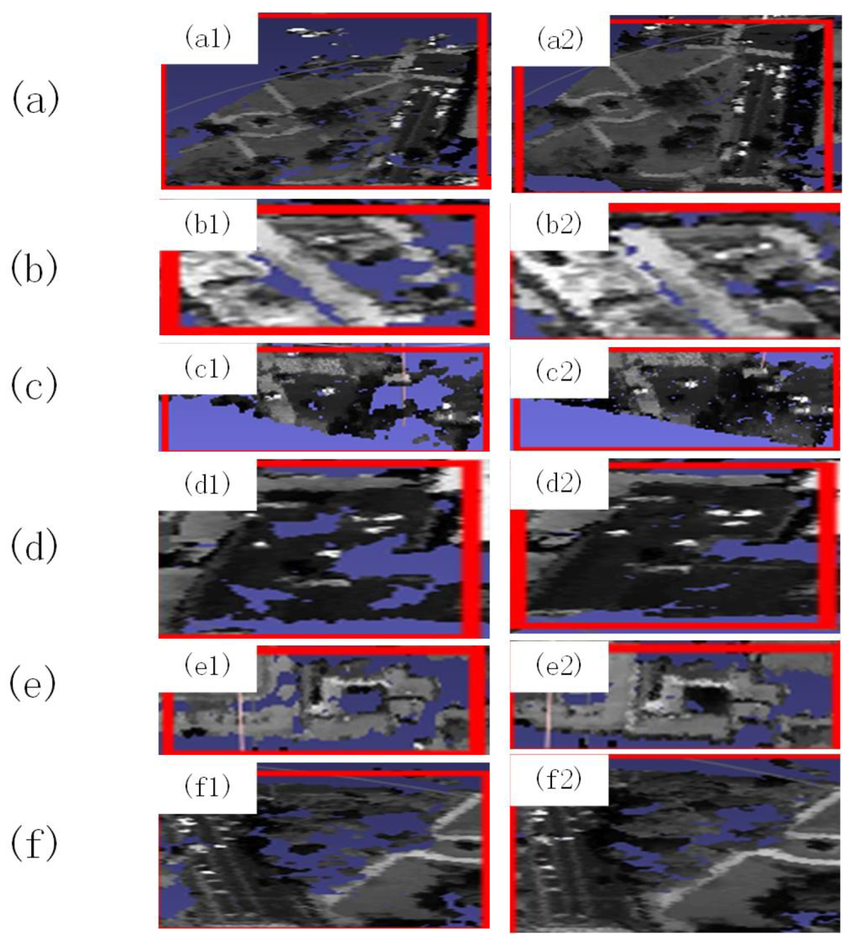
As shown, some outliers were removed after plane segmentation (Figure 13(a1,a2)). By comparing Figure 14, it can be seen that the small missed regions were almost filled, which greatly improved the matching effect. In Figure 13, three regions in boxes for each example had the best filling effect. The regions in the boxes originally contained some larger holes, and they were filled more completely than the other regions. Three regions included a roof, ground, and area containing trees. This indicates that, in addition to the roof and ground, places with many missed matching pixels, such as trees, were also filled by approximately plane fitting. The elevation of the filled area was consistent with its surroundings, indicating that most of the areas were correctly filled, as shown in Figure 15. However, the large missed matching area could not be filled. Moreover, there were some outliers in the missed matching area, which could not be removed. The elevation error and missed matching rate before and after the disparity refinement are given in Table 7. The disparity was filled using the Resolution Decoupling [25]. Its result is given in Table 7.
The proposed algorithm has two steps, the first step is super-pixel plane fitting, the second step is Mean-shift based plane segmentation, and then the disparity is corrected. Since there already exists super-pixel-based plane fitting methods, the plane segmentation method is the novelty of this paper. The disparity refinement was performed both after super-pixel plane fitting and Mean-shift based plane segmentation. The difference between the results of the two steps was clarified. In our images, the average planar super-pixel number in a block image was 203, and average 75 non-planar super-pixels were further fitted by plane segmentation algorithm. The missed matching pixel rate filled by super-pixel plane fitting was 24.9%. The average elevation error before disparity refinement was 4.05, and the standard deviation was 4.01.
After the overall disparity refinement, the missed matching rate decreased from 42.5% to 28.4%, or by one-third, which effectively improved the missed matching phenomenon. The average elevation error before disparity refinement was 4.25, and the standard deviation was 4.44. After disparity refinement, the average elevation error was 4.13, and the standard deviation was 4.06. These results indicated that the missed matching pixel rate filled by plane segmentation was 3.5%. The elevation error is slightly higher than the first step, which indicated that the error of plane segmentation was slightly higher than plane fitting. Because further plane segmentation may encounter some difficult-to-fit fragments it was more difficult. The overall elevation error was lower than that before refinement, which means that the error of the plane segmentation algorithm was still at a low level.
Outlier removal usually reduces errors, although filling a great many of the missed matching pixels may not necessarily reduce errors. The elevation error was slightly decreased, which shows the effectiveness of our outlier removal algorithm. In the case that many missed matching pixels were filled, the elevation error still decreased. This indicates that our algorithm can accurately fit planes and fill correct disparity further. The error standard deviation was also reduced, indicating that the outlier removal can shorten the error distribution interval. The resolution decoupling method can also fill a large number of missed matches. The missed matches were reduced by 1/2, but the error was increased by 1 m, and the standard deviation is also improved. The accuracy is not as good as our algorithm. In summary, the plane segmentation algorithm can further fill missed matching pixels when the elevation error was still at a low level.
4. Discussion
A disparity refinement algorithm based on mean-shift plane segmentation is proposed in this paper. Plane segmentation is performed on the initial stereo matching results combined with super-pixel segmentation. Outliers are removed, and missed matching regions are filled according to plane coefficients obtained by the plane segmentation algorithm. Thereby, the stereo matching effect is improved. The effectiveness of the plane segmentation algorithm was proved by comparing it with others on a standard plane segmentation dataset. The experiment results show that our methods outperformed PEAC in the presence of noise. On the basis of plane fitting, the proposed algorithm can segment more planes and further fill missed matching pixels while maintaining a low level of error. Besides disparity refinement, this method can also be applied to correct the optical flow field. The limitation of this method is that it is dependent on the disparity accuracy and is powerless if there are large disparity holes. These holes are mainly caused by shadows and occlusion. Future work should improve the matching algorithm, eliminate the impact of shadows and occlusion, and reduce missing pixels. Moreover, we proposed EMR and EMM to analyze and evaluate the effect of stereo matching. Experiments on the stereo matching dataset proved the effectiveness of EMR and EMM in the absence of ground truth matching results.
Author Contributions
Z.L. designed the study, and performed the experiments, and led the manuscript writing and revision. J.L. contributed to the interpretation of results and the writing of the paper, Y.Y. performed the experiments and contributed to interpret results and J.Z. contributed to the writing of the paper. All authors have read and agreed to the published version of the manuscript.
Funding
This research was funded by the National Science Foundation of China (Grant No. 51679058) and the Shandong Natural Science Foundation in China (2020–2022, No. ZR2019LZH005).
Institutional Review Board Statement
Not Applicable.
Informed Consent Statement
Not Applicable.
Data Availability Statement
Not Applicable.
Conflicts of Interest
The authors declare no conflict of interest.
References
- Jianfeng, Z.; Khot, L.R.; Bahlol, H.Y.; Boydston, R.; Miklas, P.N. Evaluation of ground, proximal and aerial remote sensing technologies for crop stress monitoring. IFAC Pap. 2016, 49, 22–26. [Google Scholar] [CrossRef]
- Kodors, S.; Rausis, A.; Ratkevics, A.; Zvirgzds, J.; Teilans, A.; Ansone, I. Real Estate Monitoring System Based on Remote Sensing and Image Recognition Technologies. Procedia Comput. Sci. 2017, 104, 460–467. [Google Scholar] [CrossRef]
- Watt, M.S.; Pearse, G.D.; Dash, J.P.; Melia, N.; Leonardo, E.M.C. Application of remote sensing technologies to identify impacts of nutritional deficiencies on forests. ISPRS J. Photogramm. Rem. Sens. 2019, 149, 226–241. [Google Scholar] [CrossRef]
- Erdélyi, R.; Wang, Y.; Guo, W.; Hanna, E.; Colantuono, G. Three-dimensional SOlar RAdiation Model (SORAM) and its application to 3-D urban planning. Sol. Energy 2014, 101, 63–73. [Google Scholar] [CrossRef]
- Mediato, J.F.; García, C.J.; Izquierdo, E.; García-Lobón, J.L.; Ayala, C.; Pueyo, E.L.; Molinero, R. Three-dimensional Reconstruction of the Caspe Geological Structure (Spain) for Evaluation as a Potential CO2 Storage Site. Energy Procedia 2017, 114, 4486–4493. [Google Scholar] [CrossRef] [Green Version]
- Kükenbrink, D.; Schneider, F.D.; Schmid, B.; Gastellu-Etchegorry, J.P.; Schaepman, M.E.; Morsdorf, F. Modelling of three-dimensional, diurnal light extinction in two contrasting forests. Agric. For. Meteorol. 2020, 296, 108230. [Google Scholar] [CrossRef]
- De Franchis, C.; Meinhardt-Llopis, E.; Michel, J.; Morel, J.M.; Facciolo, G. On stereo-rectification of pushbroom images. In Proceedings of the 2014 IEEE International Conference on Image Pro-Cessing (ICIP 2014), Paris, France, 27–30 October 2014; pp. 5447–5451. [Google Scholar]
- De Franchis, C.; Meinhardt-Llopis, E.; Michel, J.; Morel, J.M.; Facciolo, G. An automatic and modular stereo pipeline for pushbroom images. ISPRS J. Photogramm. Rem. Sens. 2014, II-3, 49–56. [Google Scholar] [CrossRef] [Green Version]
- Beyer, R.A.; Alexandrov, O.; McMichael, S. The Ames Stereo Pipeline: NASA’s open source software for deriving and processing terrain data. Earth Space Sci. 2018, 5, 537–548. [Google Scholar] [CrossRef]
- Qin, R. RPC Stereo Processor (RSP)—A software package for digital surface model and orthophoto generation from satellite stereo imagery. ISPRS J. Photogramm. Rem. Sens. 2016, III-1, 77–82. [Google Scholar] [CrossRef] [Green Version]
- Youssefi, D.; Michel, J.; Sarrazin, E.; Buffe, F.; Cournet, M.; Delvit, J.; Helguen, C.; Melet, O.; Emilien, A.; Bosman, J. Cars: A photogrammetry pipeline using dask graphs to construct a global 3d model. In Proceedings of the IGARSS—IEEE International Geoscience and Remote Sensing Symposium, Waikoloa Village, HI, USA, 16–26 July 2020. [Google Scholar]
- Michel, J.; Sarrazin, E.; Youssefi, D.; Cournet, M.; Buffe, F.; Delvit, J.; Emilien, A.; Bosman, J.; Melet, O.; Helguen, C. A new satellite imagery stereo pipeline designed for scalability, robustness and performance. ISPRS J. Photogramm. Rem. Sens. 2020, 2, 171–178. [Google Scholar] [CrossRef]
- Noh, M.J.; Howat, I.M. The Surface Extraction from TIN based Search-space Minimization (SETSM) algorithm. ISPRS J. Photogramm. Rem. Sens. 2017, 129, 55–76. [Google Scholar] [CrossRef]
- Humenberger, M.; Engelke, T.; Kubinger, W. A census- based stereo vision algorithm using modified semi-global matching and plane fitting to improve matching quality. In Proceedings of the CVPR Workshops, 2010 IEEE Computer Society Conference on Computer Vision and Pattern Recognition, San Francisco, CA, USA, 13–18 June 2010; pp. 77–84. [Google Scholar]
- Xing, M.; Sun, X.; Zhou, M.C.; Jiao, S.H.; Wang, H.T.; Zhang, X.P. On building an accurate stereo matching system on graphics hardware. In Proceedings of the ICCV Workshops, 2011 IEEE International Conference on Computer Vision Workshops, Barcelona, Spain, 6–13 November 2011; pp. 467–475. [Google Scholar] [CrossRef]
- Bleyer, M.; Gelautz, M. Graph-cut-based stereo match- ing using image segmentation with symmetrical treatment of occlusions. Signal Process. Image Commun. 2007, 22, 127–143. [Google Scholar] [CrossRef]
- Felzenszwalb, P.F.; Huttenlocher, D.P. Efficient belief propagation for early vision. Int. J. Comput. Vis. 2006, 70, 41–54. [Google Scholar] [CrossRef]
- Facciolo, G.; de Franchis, C.; Meinhardt, E. MGM: A Significantly More Global Matching for Stereovision. In Proceedings of the 2015 British Machine Vision Conference (BMVC), Swanser, UK, 7–10 September 2015. [Google Scholar]
- Heiko, H. Accurate and efficient stereo processing by semi-global matching and mutual information. In Proceedings of the 2005 IEEE Computer Society Conference on Computer Vision and Pattern Recognition (CVPR), San Diego, CA, USA, 20–26 June 2005; pp. 807–814. [Google Scholar] [CrossRef]
- Hirschmuller, H. Stereo processing by semiglobal matching and mutual information. IEEE Trans. 2007, 30, 328–341. [Google Scholar] [CrossRef] [PubMed]
- Hirschmüller, H. Semi-global matching-motivation, developments and applications. In Proceedings of the Photogrammetric Week, Stuttgart, Germany, 9–13 September 2011. [Google Scholar]
- Hirschmüller, H.; Buder, M.; Ernst, I. Memory efficient semi-global matching. ISPRS J. Photogramm. Rem. Sens. 2012, 3, 371–376. [Google Scholar] [CrossRef] [Green Version]
- Cochran, S.D.; Medioni, G. 3-d surface description from binocular stereo. IEEE Trans. Patt. Anal. Mach. Intell. 1992, 14, 994. [Google Scholar] [CrossRef]
- Zequn, J.; Pengfei, W.; Yonggen, L.; Bo, Z.; Yunchao, W.; Jiashi, F.; Wei, L. Left-Right Comparative Recurrent Model for Stereo Matching. In Proceedings of the 2018 IEEE/CVF Conference on Computer Vision and Pattern Recognition (CVPR), Salt Lake City, UT, USA, 18–23 June 2018; pp. 3838–3846. [Google Scholar] [CrossRef] [Green Version]
- Alexey, S.; El Choubassi, M.; Oscar, N. Efficient filling of disparity holes using resolution decoupling. Electron. Imaging 2016. [Google Scholar] [CrossRef]
- Jiao, J.; Wang, R.; Wang, W.; Dong, S.; Wang, Z.; Gao, W. Local stereo matching with improved matching cost and disparity refinement. IEEE MultiMedia 2014, 21, 16–27. [Google Scholar] [CrossRef]
- Huang, C.S.; Huang, Y.H.; Chan, D.Y.; Yang, J.F. Shape-reserved stereo matching with segment-based cost aggregation and dual-path refinement. EURASIP J. Image Video Process. 2020, 38, 1–19. [Google Scholar] [CrossRef]
- Yan, T.; Gan, Y.Z.; Xia, Z.Y.; Zhao, Q.F. Segment-based Disparity Refinement with Occlusion Handling for Stereo Matching. IEEE Trans. Image Process. 2019, 28, 3885–3897. [Google Scholar] [CrossRef]
- Hamzah, R.A.; Kadmin, A.F.; Ghani, S.F.A.; Hamid, M.S.; Salam, S. Disparity refinement process based on RANSAC plane fitting for machine vision applications. J. Fundam. Appl. Sci. 2018, 9, 226. [Google Scholar] [CrossRef] [Green Version]
- Zhan, Y.L.; Gu, Y.Z.; Huang, K.; Zhang, C.; Hu, K.L. Accurate image-guided stereo matching with efficient matching cost and disparity refinement. IEEE Trans. 2016, 26, 1632–1645. [Google Scholar] [CrossRef]
- Yang, Y.W.; Li, X.G.; Zhang, Y.P. Image Based Outlier Detection Algorithm for Point Cloud Reconstruction. J. Data Acquis. Process. 2018, 33, 928–935. [Google Scholar]
- Huang, X.M.; Zhang, Y.J. An O (1) disparity refinement method for stereo matching. Pattern Recognit. 2016, 55, 198–206. [Google Scholar] [CrossRef]
- Dong, Q.C.; Feng, J.Q. Outlier detection and disparity refinement in stereo matching. J. Vis. Commun. Image Represent. 2019, 60, 380–390. [Google Scholar] [CrossRef]
- Qin, R.J.; Chen, M.; Huang, X.; Hu, K. Disparity Refinement in Depth Discontinuity Using Robustly Matched Straight Lines for Digital Surface Model Generation. IEEE J. Sel. Top. Appl. Earth Obs. Remote. Sens. 2018, 12, 174–185. [Google Scholar] [CrossRef]
- Sinha, S.N.; Scharstein, D.; Szeliski, R. Efficient high-resolution stereo matching using local plane sweeps. In Proceedings of the IEEE Conference on Computer Vision and Pattern Recognition, Columbus, OH, USA, 23–28 June 2014; pp. 1582–1589. [Google Scholar]
- Vladimir, T.; Michael, S.; Ryan, F.S.; Adarsh, K.; Christoph, R.; Maksym, D.; Mirko, S.; Julien, V.; Shahram, I. SOS: Stereo Matching in O(1) with Slanted Support Windows. In Proceedings of the International Conference on Intelligent Robots and Systems, Madrid, Spain, 1–5 October 2018; pp. 6782–6789. [Google Scholar] [CrossRef]
- Geiger, A.; Roser, M.; Urtasun, R. Efficient large-scale stereo matching. In Proceedings of the Asian Conference on Computer Vision, Queenstown, New Zealand, 8–12 November 2010; Springer: Berlin/Heidelberg, Germany, 2010; pp. 25–38. [Google Scholar]
- Hou, Y.L.; Peng, J.W.; Hu, Z.H.; Peng, J.T.; Shan, J. Planarity constrained multi-view depth map reconstruction for urban scenes. ISPRS J. Photogramm. Rem. Sens. 2018, 139, 133–145. [Google Scholar] [CrossRef]
- Dong, Z.; Yang, B.S.; Hu, P.B.; Scherer, S. An efficient global energy optimization approach for robust 3D plane segmentation of point clouds. ISPRS J. Photogramm. Rem. Sens. 2018, 137, 112–133. [Google Scholar] [CrossRef]
- Vo, A.V.; Hong, L.T.; Laefer, D.F.; Bertolotto, M. Octree-based region growing for point cloud segmentation. ISPRS J. Photogramm. Rem. Sens. 2015, 104, 88–100. [Google Scholar] [CrossRef]
- Teboul, O.; Simon, L.; Koutsourakis, P.; Paragios, N. Segmentation of building facades using procedural shape priors. In Proceedings of the IEEE Conference on Computer Vision and Pattern Recognition, San Francisco, CA, USA, 13–18 June 2010; pp. 3105–3112. [Google Scholar]
- Fischler, M.A.; Bolles, R.C. Random sample consensus: A paradigm for model fitting with applications to image analysis and automated cartography. Commun. ACM 1981, 24, 381–395. [Google Scholar] [CrossRef]
- Ballard, D.H. Generalizing the Hough transform to detect arbitrary shapes. Pattern Recogn. 1981, 13, 111–122. [Google Scholar] [CrossRef] [Green Version]
- Pham, T.T.; Eich, M.; Reid, I.; Wyeth, G. Geometrically consistent plane extraction for dense indoor 3D maps segmentation. In Proceedings of the 2016 IEEE/RSJ International Conference on Intelligent Robots and Systems (IROS), Daejeon, Korea, 9–14 October 2016; pp. 4199–4204. [Google Scholar] [CrossRef]
- Yan, J.; Shan, J.; Jiang, W. A global optimization approach to roof segmentation from airborne lidar point clouds. ISPRS J. Photogramm. Rem. Sens. 2014, 94, 183–193. [Google Scholar] [CrossRef]
- Isack, H.; Boykov, Y. Energy-based geometric multi-model fitting. Int. J. Comput. Vis. 2012, 97, 123–147. [Google Scholar] [CrossRef] [Green Version]
- Andrew, D.; Anton, O.; Hossam, N.I.; Yuri, B. Fast Approximate Energy Minimization with Label Costs. In Proceedings of the 2010 IEEE Conference on Computer Vision and Pattern Recognition (CVPR), San Francisco, CA, USA, 13–18 June 2010; Volume 96, pp. 1–27. [Google Scholar]
- Liu, M.Y.; Tuzel, O.; Ramalingam, S.; Rama, C. Entropy rate superpixel segmentation. In Proceedings of the 24th IEEE Conference on Computer Vision and Pattern Recognition(CVPR), Colorado Springs, CO, USA, 20–25 June 2011; pp. 2097–2104. [Google Scholar] [CrossRef]
- Feng, C.; Taguchi, Y.; Kamat, V.R. Fast plane extraction in organized point clouds using agglomerative hierarchical clustering. In Proceedings of the 2014 IEEE International Conference on Robotics and Automation (ICRA), Hong Kong, China, 1–7 June 2014. [Google Scholar] [CrossRef]
Figure 1.
Flowchart of disparity refinement.

Figure 2.
Circle moving process(the red circle is the mean value point): (a) First clustering. (b) Second clustering.
Figure 2.
Circle moving process(the red circle is the mean value point): (a) First clustering. (b) Second clustering.

Figure 3.
The EMMs of some images: (a) The left image of Motorcycle and Piano. (b) MGM. (c) SGM. (d) GC. (e) Ground truth.
Figure 3.
The EMMs of some images: (a) The left image of Motorcycle and Piano. (b) MGM. (c) SGM. (d) GC. (e) Ground truth.

Figure 4.
Wrong matches in the ground truth images: (a) The left part of the Adirondack image and playroom image. (b) The ground truth. (c) The SGM algorithm. (d) The error part of the ground truth. (e) The SGM corresponding to the matching graph.
Figure 4.
Wrong matches in the ground truth images: (a) The left part of the Adirondack image and playroom image. (b) The ground truth. (c) The SGM algorithm. (d) The error part of the ground truth. (e) The SGM corresponding to the matching graph.

Figure 5.
Edge matching map of remote sensing images: (a) Left image. (b) Right image. (c) The MGM algorithm. (d) The SGM algorithm.
Figure 5.
Edge matching map of remote sensing images: (a) Left image. (b) Right image. (c) The MGM algorithm. (d) The SGM algorithm.

Figure 6.
The plane fitting effects of different algorithms: (a) Point cloud image. (b) The PEAC algorithm. (c) The proposed algorithm (the first line is the Gaussian curved surface, the second line is the decreasing sine curved surface, and the third line represents the two examples of SegComp).
Figure 6.
The plane fitting effects of different algorithms: (a) Point cloud image. (b) The PEAC algorithm. (c) The proposed algorithm (the first line is the Gaussian curved surface, the second line is the decreasing sine curved surface, and the third line represents the two examples of SegComp).

Figure 7.
The labeled ground truth: (a) The ground truth of Figure 6(a3). (b) The ground truth of Figure 6(a4).

Figure 8.
Anti-noise performance parameters: (a) ‘Salt’ noise parameters. (b) Gaussian noise parameters.
Figure 8.
Anti-noise performance parameters: (a) ‘Salt’ noise parameters. (b) Gaussian noise parameters.

Figure 9.
The plane fitting effect after adding noise: (a) The point cloud image after adding noise. (b) The PEAC algorithm result. (c) The mean-shift result.
Figure 9.
The plane fitting effect after adding noise: (a) The point cloud image after adding noise. (b) The PEAC algorithm result. (c) The mean-shift result.

Figure 10.
Plane fitting results of remote sensing images: (a) The left images. (b) The disparity images. (c) The plane segmentation images (The first line corresponds to example 1 and the second line to example 2).
Figure 10.
Plane fitting results of remote sensing images: (a) The left images. (b) The disparity images. (c) The plane segmentation images (The first line corresponds to example 1 and the second line to example 2).

Figure 11.
Segmentation results of some super-pixels in Block Image 1: (a) 3D maps of super-pixel disparity. (b) 3D maps of segmented planes. (c) Segmented label images. (d) Segmented label images after filling missed matching. (e) Segmented edge images (Columns 1–3 correspond to the three super-pixels in the rectangles in the first image of Figure 10c).

Figure 12.
Segmentation results of some super-pixels in Block Image 2: (a) 3D maps of super-pixel disparity. (b) 3D maps of segmented planes. (c) Segmented label images. (d) Segmented label images after filling missed matching. (e) Segmented edge images (Columns 1–3 correspond to the three super-pixels in the rectangles in the first image of Figure 10c).

Figure 13.
The results of disparity refinement: (a1) Outlier removal effect of Example 1. (a2) Outlier removal effect of Example 2. (b1) Original disparity of Example 1. (b2) Disparity of Example 1 after filling. (c1) Original disparity of Example 2. (c2) Disparity of Example 2 after filling. (d1) Original point cloud of Example 1. (d2) Point cloud of Example 1 after filling. (e1) Original point cloud of Example 2. (e2) Point cloud of Example 2 after filling.

Figure 14.
An enlarged view of the boxes in Figure 13: (a1) Box 1 in Figure 13(b1). (a2) Box 1 in Figure 13(b2). (b1) Box 2 in Figure 13(b1). (b2) Box 2 in Figure 13(b2). (c1) Box 3 in Figure 13(b1). (c2) Box 3 in Figure 13(b2). (d1) Box 1 in Figure 13(c1). (d2) Box 1 in Figure 13(c2). (e1) Box 2 in Figure 13(c1). (e2) Box 2 in Figure 13(c2). (f1) Box 3 in Figure 13(c1). (f2) Box 3 in Figure 13(c2).

Figure 15.
An enlarged view of the boxes in Figure 13: (a1) Box 1 in Figure 13(d1). (a2) Box 1 in Figure 13(d2). (b1) Box 2 in Figure 13(d1). (b2) Box 2 in Figure 13(d2). (c1) Box 3 in Figure 13(d1). (c2) Box 3 in Figure 13(d2). (d1) Box 1 in Figure 13(e1). (d2) Box 1 in Figure 13(e2). (e1) Box 2 in Figure 13(e1). (e2) Box 2 in Figure 13(e2). (f1)Box 3 in Figure 13(e1). (f2) Box 3 in Figure 13(e2).


Table 1.
Matching results of MiddEval3.
| MGM | SGM | GC | Ground Truth | ||||
|---|---|---|---|---|---|---|---|
| Image Name | EMR | MAR | EMR | MAR | EMR | MAR | EMR |
| Adirondack | 50.4% | 19.7% | 83.1% | 25.4% | 50.9% | 16.2% | 64.5% |
| ArtL | 9.4% | 2.2% | 58.8% | 9.7% | 39.0% | 0 | 53.2% |
| Jadeplant | 18.5% | 1.6% | 82.6% | 19.2% | 48.5% | 12.1% | 54.9% |
| Motorcycle | 52.9% | 24.7% | 86.0% | 45.1% | 49.0% | 8.5% | 63.7% |
| Piano | 51.5% | 17.3% | 86.4% | 28.4% | 49.7% | 4.7% | 67.4% |
| Pipes | 34.0% | 8.1% | 75.7% | 31.2% | 37.3% | 5.4% | 49.3% |
| Playroom | 38.4% | 11.9% | 81.9% | 18.5% | 41.5% | 1.7% | 55.5% |
| Playtable | 48.3% | 11.2% | 86.5% | 37.7% | 40.6% | 6.1% | 53.3% |
| Recycle | 38.9% | 12.7% | 82.6% | 38.1% | 47.8% | 21.2% | 62.1% |
| Shelves | 57.4% | 14.9% | 89.2% | 25.1% | 34.9% | 0.1% | 66.7% |
| Teddy | 58.6% | 34.5% | 84.6% | 51.4% | 50.2% | 13.5% | 69.0% |
| Vintage | 30.2% | 3.1% | 81.6% | 9.2% | 29.4% | 1.3% | 46.3% |
| Mean | 40.7% | 13.5% | 81.6% | 28.2% | 43.2% | 7.6% | 58.8% |
Table 2.
The EMR of the block images in Figure 5.
Table 2.
The EMR of the block images in Figure 5.
| Number | EMR of MGM | Elevation Error | EMR of SGM | Elevation Error |
|---|---|---|---|---|
| 1 | 44.2% | 5.27 | 42.1% | 8.98 |
| 2 | 46.7% | 3.69 | 47.2% | 5.44 |
| 3 | 44.8% | 4.87 | 41.3% | 10.32 |
| 4 | 45.1% | 4.82 | 48.6% | 5.58 |
| Mean | 45.3% | 4.66 | 44.8% | 7.58 |
Table 3.
The average EMR and elevation error of all the block images.
| EMR of MGM | Elevation Error | EMR of SGM | Elevation Error | |
|---|---|---|---|---|
| Value | 42.1% | 4.25 | 40.2% | 7.17 |
Table 4.
Plane segmentation error and estimated plane number.
| Error | Number | ||||
|---|---|---|---|---|---|
| PEAC | Mean-Shift | PEAC | Mean-Shift | Ground Truth | |
| Self-built dataset | 3.21 | 0.20 | |||
| SegComp | 1.13 | 0.13 | 4 + 10 = 14 | 10 + 20 = 30 | 6 + 20 = 26 |
Table 5.
The number of plane super-pixels estimated using different error thresholds and density thresholds.
Table 5.
The number of plane super-pixels estimated using different error thresholds and density thresholds.
| Error Threshold | 0.8 | 1.0 | 1.2 | 1.4 | 1.5 | 1.6 | 1.7 | 1.8 | |
|---|---|---|---|---|---|---|---|---|---|
| Density Threshold | |||||||||
| 0.7 | 647 | 712 | 778 | 809 | 826 | 844 | 879 | 883 | |
| 0.6 | 730 | 800 | 861 | 883 | 905 | 931 | 953 | 970 | |
| 0.5 | 795 | 874 | 962 | 970 | 988 | 1014 | 1031 | 1040 | |
Table 6.
Determination of Bandwidth threshold and inlier point threshold.
| Bandwidth | Plane Fitting Error | Inlier Point Threshold | Elevation Error |
|---|---|---|---|
| 3 | 3.86 | 5 | 4.25 |
| 4 | 3.60 | 6 | 4.18 |
| 5 | 3.51 | 7 | 4.26 |
| 6 | 3.78 | 8 | 4.37 |
| 7 | 4.15 | 9 | 4.57 |
Table 7.
Statistics of the elevation error and the missed matching rate.
| Mean | Standard Deviation | Missed Matching Rate | |
|---|---|---|---|
| Before disparity refinement | 4.25 | 4.44 | 42.5% |
| After super-pixel plane fitting refinement | 4.05 | 4.01 | 24.9% |
| After disparity refinement | 4.13 | 4.06 | 28.4% |
| Resolution Decoupling | 5.19 | 5.01 | 21.9% |
Publisher’s Note: MDPI stays neutral with regard to jurisdictional claims in published maps and institutional affiliations. |
© 2021 by the authors. Licensee MDPI, Basel, Switzerland. This article is an open access article distributed under the terms and conditions of the Creative Commons Attribution (CC BY) license (https://creativecommons.org/licenses/by/4.0/).
Share and Cite
MDPI and ACS Style
Li, Z.; Liu, J.; Yang, Y.; Zhang, J. A Disparity Refinement Algorithm for Satellite Remote Sensing Images Based on Mean-Shift Plane Segmentation. Remote Sens. 2021, 13, 1903. https://0-doi-org.brum.beds.ac.uk/10.3390/rs13101903
AMA Style
Li Z, Liu J, Yang Y, Zhang J. A Disparity Refinement Algorithm for Satellite Remote Sensing Images Based on Mean-Shift Plane Segmentation. Remote Sensing. 2021; 13(10):1903. https://0-doi-org.brum.beds.ac.uk/10.3390/rs13101903
Chicago/Turabian StyleLi, Zhihui, Jiaxin Liu, Yang Yang, and Jing Zhang. 2021. "A Disparity Refinement Algorithm for Satellite Remote Sensing Images Based on Mean-Shift Plane Segmentation" Remote Sensing 13, no. 10: 1903. https://0-doi-org.brum.beds.ac.uk/10.3390/rs13101903
Note that from the first issue of 2016, this journal uses article numbers instead of page numbers. See further details here.