
A Universal Automatic Bottom Tracking Method of Side Scan Sonar Data Based on Semantic Segmentation


1
School of Geodesy and Geomatics, Wuhan University, Wuhan 430079, China
2
Institute of Marine Science and Technology, Wuhan University, Wuhan 430079, China
3
Department of Artificial Intelligence and Automation, School of Electrical Engineering and Automation, Wuhan University, Wuhan 430072, China
*
Author to whom correspondence should be addressed.
Remote Sens. 2021, 13(10), 1945; https://0-doi-org.brum.beds.ac.uk/10.3390/rs13101945
Submission received: 8 April 2021
/
Revised: 6 May 2021
/
Accepted: 14 May 2021
/
Published: 17 May 2021
(This article belongs to the Special Issue Deep Learning for Radar and Sonar Image Processing)
Abstract
:Determining the altitude of side-scan sonar (SSS) above the seabed is critical to correct the geometric distortions in the sonar images. Usually, a technology named bottom tracking is applied to estimate the distance between the sonar and the seafloor. However, the traditional methods for bottom tracking often require pre-defined thresholds and complex optimization processes, which make it difficult to achieve ideal results in complex underwater environments without manual intervention. In this paper, a universal automatic bottom tracking method is proposed based on semantic segmentation. First, the waterfall images generated from SSS backscatter sequences are labeled as water column (WC) and seabed parts, then split into specific patches to build the training dataset. Second, a symmetrical information synthesis module (SISM) is designed and added to DeepLabv3+, which not only weakens the strong echoes in the WC area, but also gives the network the capability of considering the symmetry characteristic of bottom lines, and most importantly, the independent module can be easily combined with any other neural networks. Then, the integrated network is trained with the established dataset. Third, a coarse-to-fine segmentation strategy with the well-trained model is proposed to segment the SSS waterfall images quickly and accurately. Besides, a fast bottom line search algorithm is proposed to further reduce the time consumption of bottom tracking. Finally, the proposed method is validated by the data measured with several commonly used SSSs in various underwater environments. The results show that the proposed method can achieve the bottom tracking accuracy of 1.1 pixels of mean error and 1.26 pixels of standard deviation at the speed of 2128 ping/s, and is robust to interference factors.
1. Introduction
As a category of active sonar, SSS has been widely used in underwater target detection [1,2,3,4,5,6] and benthic habitat mapping [7,8,9,10,11,12] over the last decades due to its low price and ability to efficiently obtain a high-resolution acoustic image of large areas of the sea floor [13]. However, raw SSS imagery presents severe across-track geometric distortions, known as slant range distortions. They occur because sonar systems actually measure the traveling time of a transmitted pulse from the transducer to the target and back to the transducer [14]. Without slant range correction, near-range areas are more compressed than far-range areas, and follow-up radiometric correction cannot be caried out properly, which causes serious problems in applications of underwater target detection, seabed sediment classification, and image interpretation. To solve the problem, the height of sonar from seabed needs to be estimated by finding the boundary, namely bottom line, between WC area and seabed area with a technique called bottom tracking.
Traditionally, bottom line is extracted manually which is time-consuming and unreliable because its accuracy depends on the experience of the operator. Many researchers have studied the automatic methods of bottom tracking. Among them, the threshold methods are widely used in commercial software such as EdgeTech Discover, but the minimum altitude and the minimum tracking range need to be preset to improve the tracking accuracy [15]. In order to weaken the influence of image noises on bottom tracking, Woock used the median filter to reduce the speckle noise in SSS waterfall images and the first bottom return (FBR) was detected as the first occurrence of two adjacent sonar samples that were more than the empirically determined threshold apart from the mean value of the ping. Then the Kalman filter was applied to smooth the detected FBR sequence and limit the influence of outliers [16]. Zhao et al. proposed a comprehensive method for bottom tracking based on the seabed continuous variation and the symmetry assumption, which can obtain robust results even in the complicated measuring environment [17]. Two methods were proposed to detect the FBRs in [18]. The first is based on smoothing cubic spline regression and the second is based on a moving average filter to detect signal variations. Shih et al. proposed an adaptive sea bottom tracking method combining image filtering, image segmentation, and edge detection technology, and achieved high accuracy [19]. A new method taking full advantage of the spatial distribution characteristics of the sea bottom line was proposed in [20], in which the points density clustering and the chains seeking were two core processes, and has good stability and anti-interference ability in a complex water environment. The above traditional methods improve the efficiency and reliability of the sea bottom line extraction to some extent, but require setting threshold parameters manually. Besides, in these traditional methods, the detection of sea bottom lines in each ping is merely based on the local echo intensity mutation feature, so they are susceptible to interference from noise and strong echoes in the WC area, and a complex optimization process is often required, which makes it difficult for these methods to be fully automated.
Recently, a high-accuracy and real-time bottom tracking method based on 1D-CNN has been proposed through traversing each ping, and the bottom data sequence fragments can be recognized accurately with the trained model [21]. By means of the powerful feature extraction ability of the neural network, the method is quite robust to the effects of noises, seabed textures, and artificial targets. However, 1D-CNN is unable to obtain the information of adjacent pings, and may become inefficient when there exists missing pings and excessive suspended solids in WC, and also requires additional optimization process. Moreover, traversing each sampling points requires the whole network to do a complete forward calculation. Although the narrow search range is used, the 1D-CNN method may still be time-consuming.
As a mature technology, deep learning (DL) is widely used in the field of image processing. Some excellent artificial neural network (ANN) models have been verified on large datasets, and the performance is much better than traditional methods [22,23,24]. ANNs can learn abstract features from images and deal with various complex scenes, therefore, they have been successfully applied to tackle SSS data measured in complex underwater environments [25,26,27,28]. Among them, the semantic segmentation network is used to classify each pixel in the image. Since some of these networks can not only effectively extract local features, but also have the ability to acquire contextual information, they have high segmentation accuracy and strong resistance to object occlusion [29]. In addition, because adjacent pixels in the image share part of the calculations, the calculation efficiency of semantic segmentation network is high, and real-time semantic segmentation of SSS data has been achieved [30].
In view of the excellent characteristics of the semantic segmentation network, we propose a universal automatic bottom tracking method based on semantic segmentation in this paper. First, the SSS imaging principle and the problems encountered in bottom tracking are analyzed. Second, according to the characteristics of SSS images, a symmetrical information synthesis module is well-designed and added to DeepLabv3+, and then the network is trained with the specially designed dataset for segmenting the SSS images into WC and seabed parts. Third, the trained model is applied to the segmentation of SSS waterfall image and the bottom lines are extracted with a fast search algorithm. Finally, the proposed method is proved by the SSS data collected by different SSS systems under various underwater environments.
2. Materials and Methods
This chapter begins with a brief introduction of the operating principle of SSS and the factors affecting sea bottom tracking are analyzed. Then, the accurate segmentation of SSS images based on the semantic segmentation network is introduced in detail. Finally, the bottom tracking method with the trained model is presented.
2.1. SSS Working Operating and Influencing Factors
2.1.1. SSS Working Principle
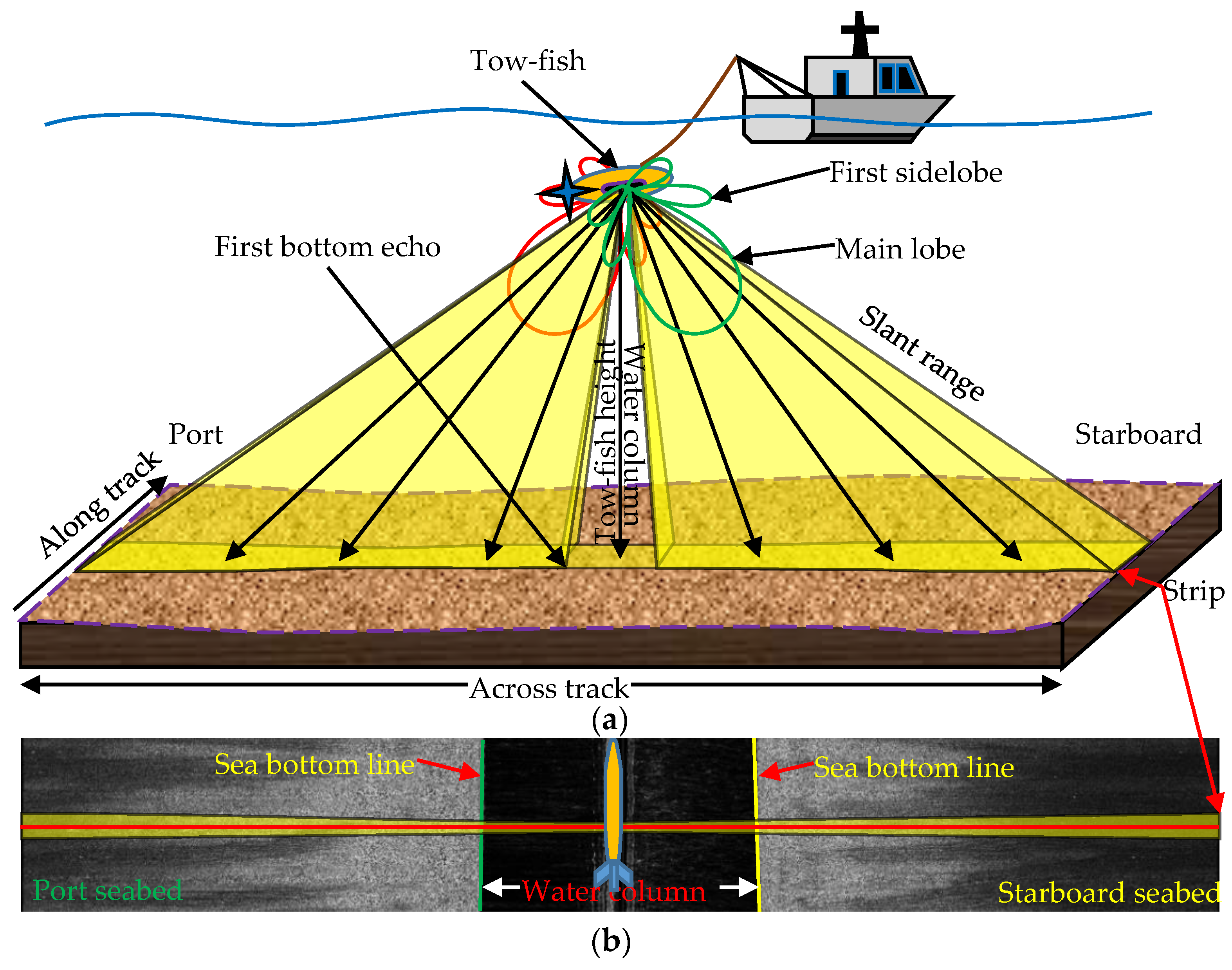
The working principle of SSS is shown in Figure 1. Usually, a side-scan sonar has two transducer arrays installed on each sides of the tow-fish and is towed behind a survey ship with a cable near the bottom. During the measurement, each transducer array sends out a sound beam which is broad in the vertical plane and narrow in the horizontal plane periodically at the same time. SSS starts to record the echo signal immediately as soon as the acoustic wave is transmitted. Since the sound wave propagates in the water first, the echo signals received at the beginning are mainly background noises and reflections from suspended solids in the water [31]. When the sound wave strikes the seabed, a series of strong echoes will be generated, which reflect the changes of seabed sediment and topography. Each beam will cover a thin strip of sea bottom across the track. The height of the tow-fish can be estimated according to the time when the first bottom echo appears and sound velocity in water. The echo sequence obtained after each emission is called a ping and successive pings are arranged in order to form a waterfall image.
A typical SSS waterfall image is shown as (B) in Figure 1. The left half of the waterfall image is formed by the data measured on the port side, and the right half is formed by the data measured on the starboard side. The darker area in the middle is known as the WC area, and the outer area is the seabed area. Each row in the waterfall image represents a ping of SSS data produced by a transmitted sound wave. Bottom lines are the boundaries of the WC area and seabed area with two important characteristics of symmetry and continuity [17]. Extracting the bottom line is an important step of SSS data processing, which directly affects the quality of data processing results and follow-up applications.
2.1.2. Influencing Factors
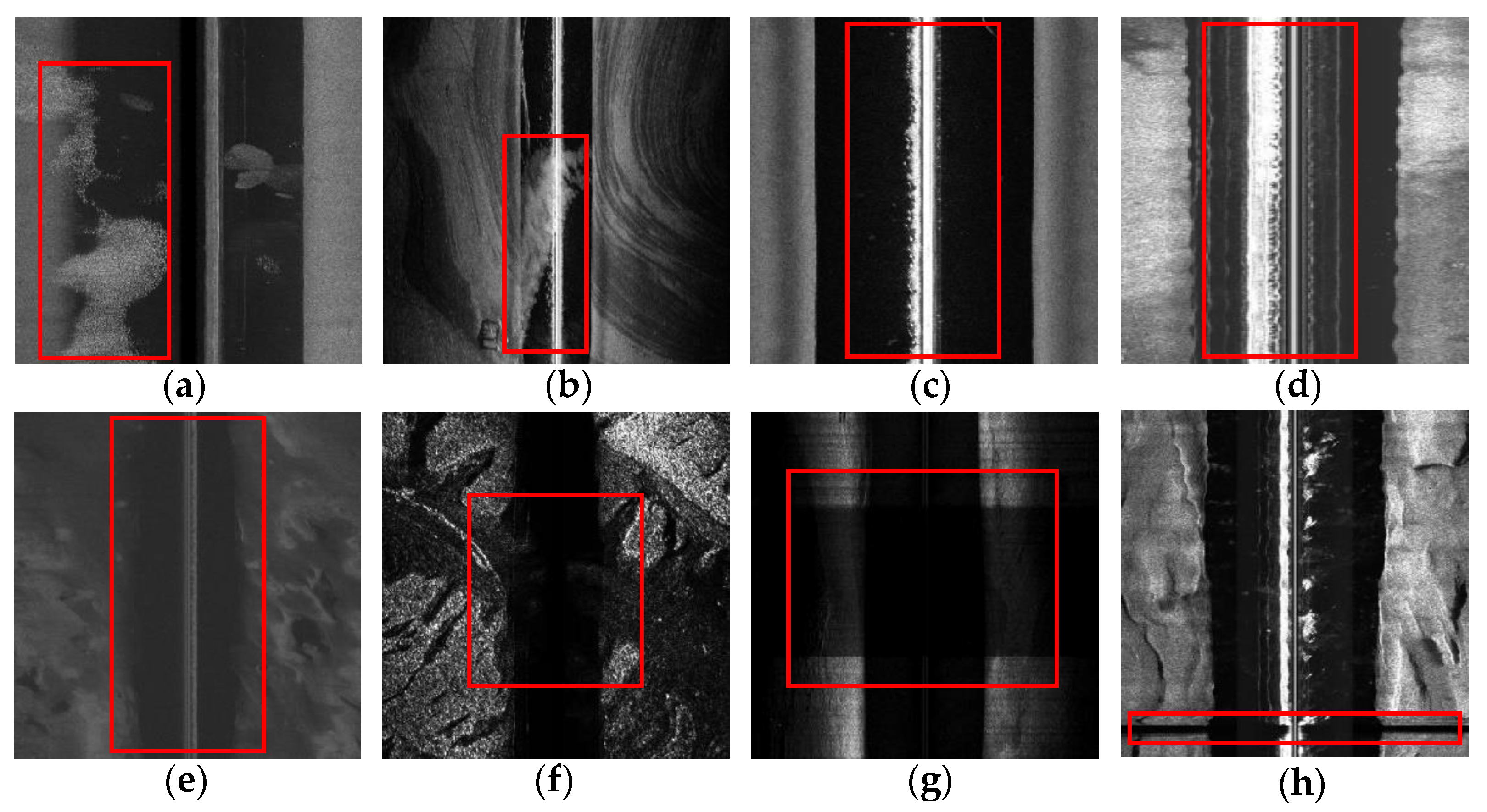
Ideally, there are no intense echoes in the WC area, and the first strong echo would be generated when the sound waves first reach the sea floor. The FBRs can be easily located by traversing the echo sequence of each ping until an echo stronger than a predefined threshold is found. However, there are many factors that may bring trouble to the accurate detection of the FBRs during the actual measurement. Some common issues affecting the bottom-tracking are shown in Figure 2, which can be classified into the following categories.
- Strong echoes in the WC area: When there are massive, suspended solids (fish schools, methane plumes, water weeds, etc.) beneath the sonar, the strong echoes from them will come earlier than those from the seabed, as shown in Figure 2a,b. Besides, if the tow-fish is towed too closely to the survey vessel, the bubbles in the wake will also produce intense echoes in the WC area as shown in Figure 2c. In addition to the above external factors, if the sidelobe energy level of SSS itself is not suppressed well, even though is low, the echoes from sea surface will reflected to the sonar and cause strong echo signals in the SSS data records due to the shorter propagation distance [17], as shown in Figure 2d. Strong echoes in the WC area will make it difficult to judge the correct position of FBRs only by simple local feature extraction operators, for example, gradient features.
- Low contrast between WC area and seabed area: High-frequency sound waves are absorbed quickly and scattered in high turbidity water. The SSS image obtained under this condition will have poor contrast and high noise, as shown in Figure 2e. In addition, if the seabed at the nadir of the sonar is covered by strong absorption sediments, most of the energy will be absorbed and the FBRs will be very weak, as shown in Figure 2f. Low contrast between the WC area and seabed area will greatly increase the difficulty of FBR recognition by thresholding methods.
- Unknown gains: During the field survey, the operators sometimes adjust the time varying gain (TVG) for optimal visualization of echo signals, resulting in overall brightness differences between the pings collected at different time periods, as shown in Figure 2g. However, the gain information is sometimes not stored, which makes it impossible to detect the position of the sea bottom line stably using a single fixed threshold.
- Missing pings: If there are dense bubbles in the water around the sonar, acoustic pulses emitted by the transducer arrays will be completely blocked, making the sonar unable to receive effective echo signals, which will be against the assumption that the sea bottom line is continuous, and lead to the failure of some dynamic filtering optimization algorithms such as the Kalman filter.
- Other: Artificial structures (artificial reef, sunken wrecks, etc.) and raised rocks on the sea floor will also cause strong echoes in the WC area, affecting the judgment of the sea bottom line.
2.2. Semantic Segmentation Model Establishment of SSS Images
2.2.1. Re-Quantization of Raw SSS Data
The output from the sonar hardware does not always follow the same quantization schemes (i.e., it can be sampled with an 11-bit or a 64-bit system) [14]. To obtain a unified semantic segmentation model, the echo intensity values stored with different bit lengths need to be re-quantized to the same value range. The re-quantization formula can be expressed as follows:
where m is the original number of bits; n is the new number of bits (i.e., n = 8 for a range 0–255 is adopted in this article). It can be seen from the formula that there are no preset parameters and no manual intervention is needed. After re-quantification, the successive pings are arranged in order to form a waterfall image.
2.2.2. Collecting Samples
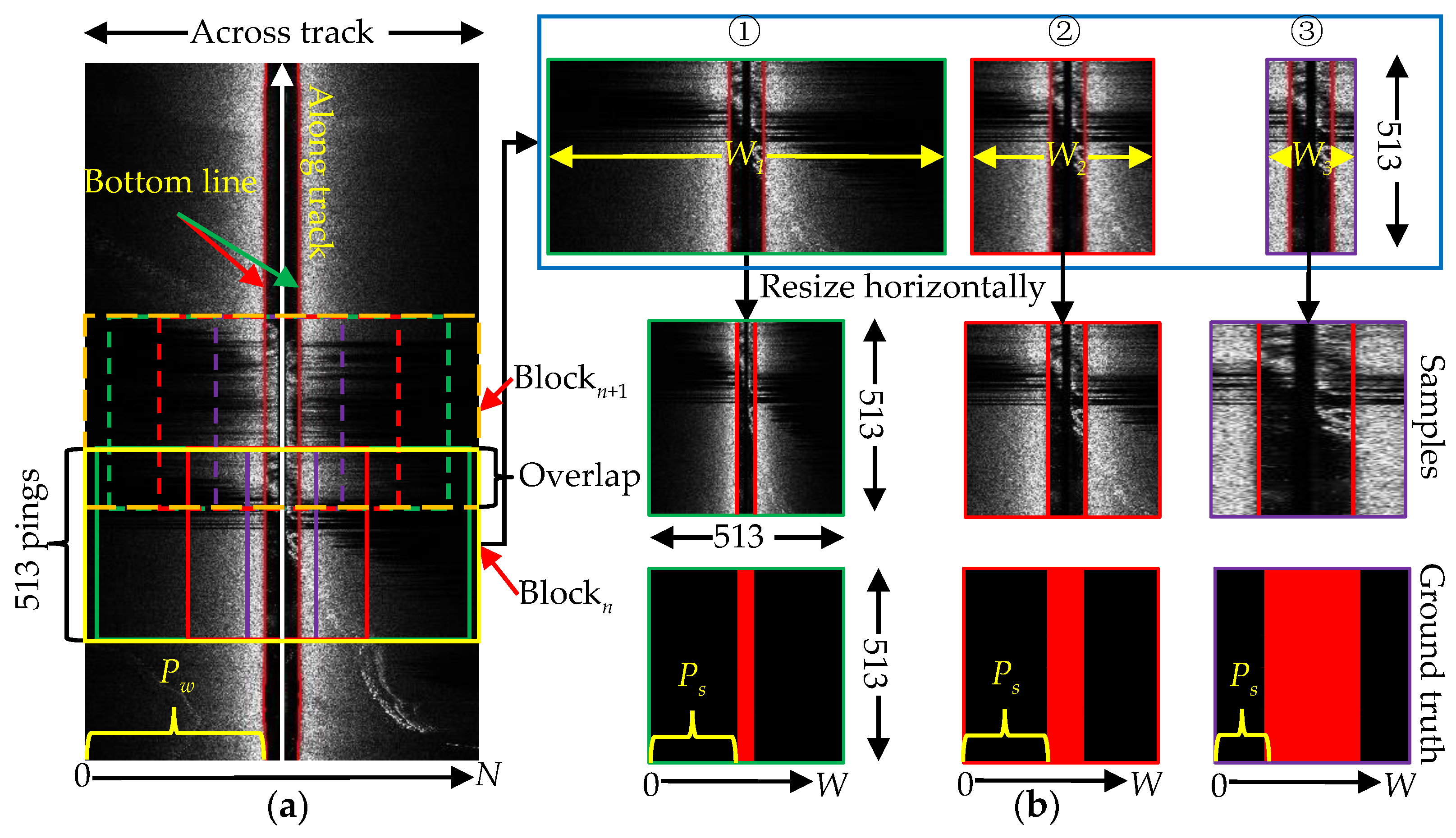
The original waterfall images usually have a large size and is not suitable to be used as training samples directly. Therefore, it is necessary to divide the original waterfall images into image blocks of the same height along the survey line. In order to obtain more samples, there is 30% overlap between adjacent blocks. For each block, three sub image blocks with different widths are obtained by randomly cutting off equal width of outer seabed image respectively. Then, the width of the sub-image block is scaled to the same size as the height. This serves two purposes: one is to balance the number of pixels in the WC area and the seabed area, and the other is to enhance the adaptability of the network to the SSS waterfall images with different proportions of WC area. A more intuitive description is displayed in Figure 3.
Each pixel of the samples needs to be labeled with a category, and a fast sample labeling method is given as the following 3 steps.
Step 1: The bottom lines of the original SSS waterfall image can be extracted directly by hand or existing automatic algorithms assisted by manual optimization.
Step 2: According to the sample generation process and the bottom tracking results obtained in Step 1, the position of sea bottom lines Ps in the sample can be calculated by Formula (2).
where N is the total number of samples in each ping, W is the width of the sample, Wi is the width of the i-th of three sub image blocks, Pw is the position of sea bottom lines in original waterfall image. All the variables take the lower-left corner of the image as the origin and are positive to right and upward.
Step 3: The pixels between the port and starboard sea bottom lines in the sample are automatically labeled as WC area and the rest as seabed area by the computer. Labeling results are used as the ground truth for network training.
2.2.3. Symmetrical Information Synthesis Module (SISM)
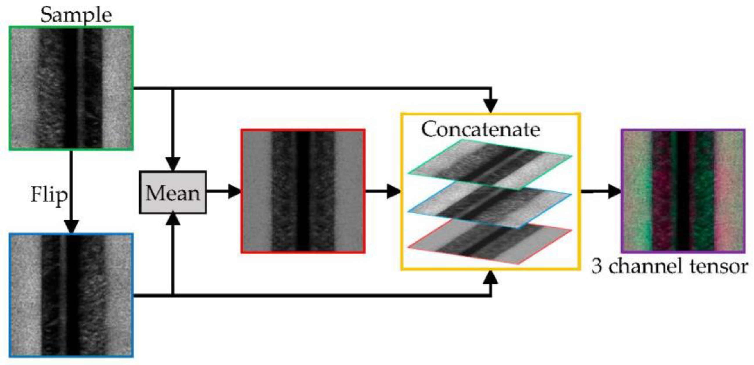
Although modern semantic segmentation neural network architectures can achieve high segmentation accuracy by encoding rich contextual information and refining the segmentation results along object boundaries [29], they cannot effectively learn the symmetry of sea bottom lines. Therefore, when there are strong interferences in consecutive pings on one side of the waterfall image, the existing networks are unable to segment the image correctly on the disturbed side by synthesizing the useful information on the other side. In order to weaken the interference of strong echoes in WC area and give the network the capability of considering the corresponding echo information of port and starboard at the same time, an efficient module is designed for the semantic segmentation network (Figure 4).
According to the calculation principle of convolution neural network (CNN) [32], the filter bank can extract the features of each input channel and synthesize the information obtained from different channels. Therefore, we can give the network the capability of taking advantage of the symmetry of sea bottom lines by flipping the raw sample across the track as the second input channel. In addition, if the strong echoes only appear on one side of the WC area, then they can be suppressed by averaging the corresponding pixel values on the original images and flipped images, and the reflection intensity from seabed on both sides is usually similar and won’t change much after taking the average. As a result, the contrast between the WC area and the seabed area is enhanced in the mean image and the boundaries become sharper. The mean image is used to provide supplementary information as the third input channel for the network. Eventually, a single-channel grayscale image sample is transformed into a 3-channel tensor. This module does not need any prior parameters, and is independent of the main body of image segmentation network, so it can be flexibly combined with various networks.
2.2.4. Semantic Segmentation Network Architecture
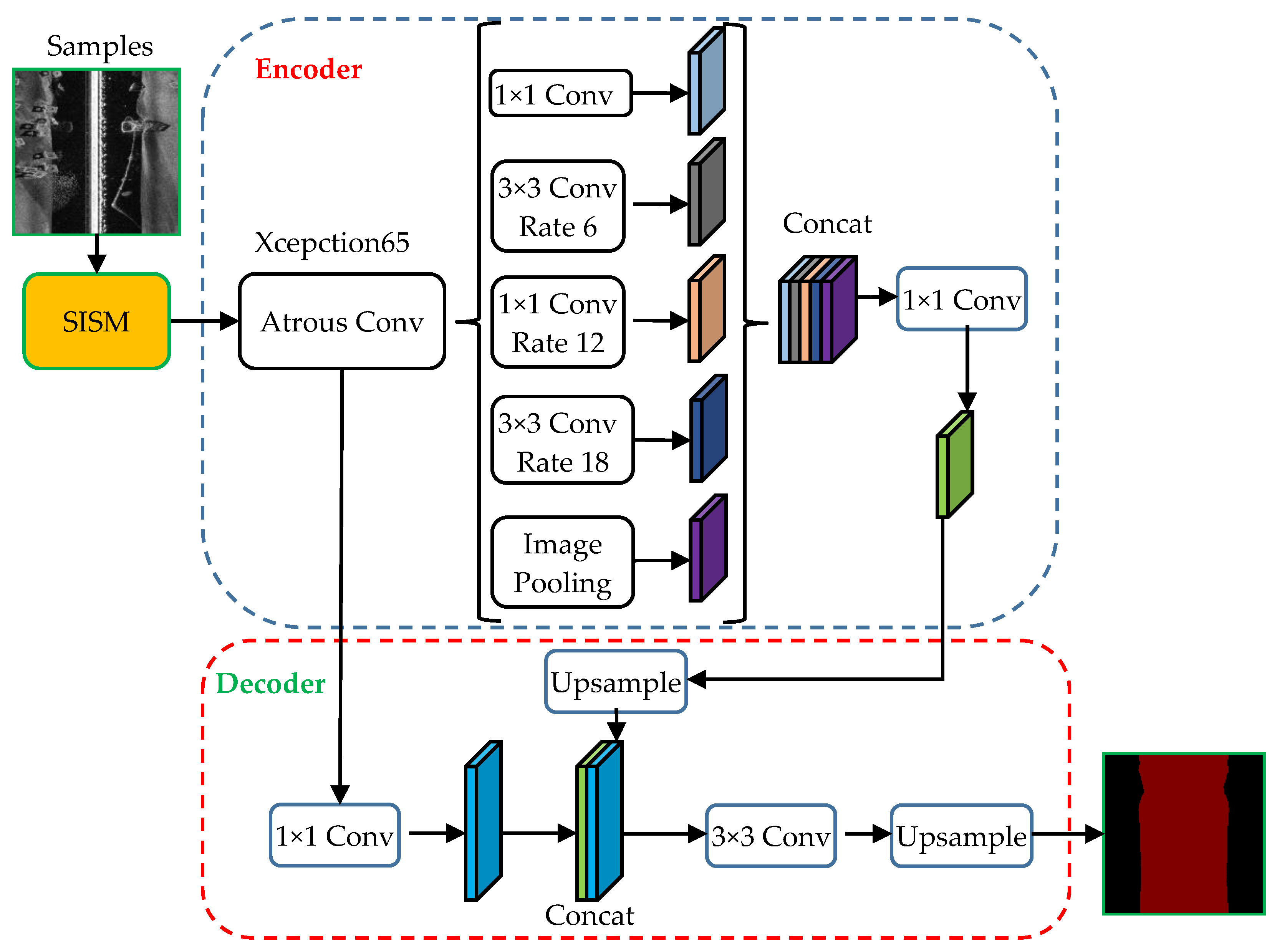
The semantic segmentation network realizes image segmentation by classifying each pixel of the image. Currently, there are many excellent image semantic segmentation neural networks (U-Net [33], PSPNet [34], DeepLabv3+ [29], etc.), whose effectiveness has been verified on large scale datasets. So, we can use the pre-trained weights on bigger datasets to train our own models in less time and with fewer samples. Among those semantic segmentation networks, DeepLabv3+ has higher segmentation accuracy and computational efficiency, therefore, is adopted to segment the SSS waterfall image into WC area and seabed area. The SISM is added to the head of DeepLabv3+, as shown in Figure 5.
DeepLabv3+ contains an encoder-decoder structure where the encoder module is used to encode the rich contextual information and the decoder module is adopted to recover sharper object boundaries. Atrous convolution with different rates is applied to extract the encoder features at an arbitrary resolution, depending on the available computation resources. A more detailed description of DeepLabv3+ can be found in paper [29]. For the segmentation of SSS data, multi-scale contextual information not only helps to weaken the influence of local anomalies in each ping, but also restricts the classification of echoes with information from adjacent pings. With the object boundary recovery ability, more accurate boundaries between WC area and seabed area can be obtained from the segmentation results. These two excellent characteristics make DeepLabv3+ quite suitable to segment the SSS waterfall images in various situations and obtain a more robust result than those method of handling each ping separately, such as 1D-CNN network [15].
All the samples are first processed by the designed SISM, and then input into the network for end-to-end training. The cross-entropy loss function is adopted to calculate the difference between the predicted results and the ground truth. For each sample, the loss is calculated as follows:
where is the predicted label, is the ground truth. For the binary segmentation of SSS waterfall image in this paper, when the pixels belong to seabed area and 1 for the WC area.
When the loss value tends to be stable and the segmentation accuracy on validation set no longer increases, then the well-trained model is saved for the SSS image segmentation and the bottom tracking procedure.
2.3. Bottom Tracking with the Trained Model
2.3.1. Patch-Wise Coarse Segmentation
The neural network used in this paper is a fully convolutional network (FCN). In theory, as long as the computer is powerful enough, the well-trained model in Section 2.2 can be directly used to segment the high resolution SSS waterfall images without resizing the images. However, most people’s computers cannot meet the requirements. Besides, the range of the network’s receptive field is limited, and the original SSS waterfall images need to be scaled to the same size as the training sample across the track, so that the mod-el can better distinguish the WC area and the seabed area. Therefore, in order to improve the practicability of the method and get better results, a patch-wise segmentation strategy is proposed in this paper. The process is shown schematically in Figure 6.
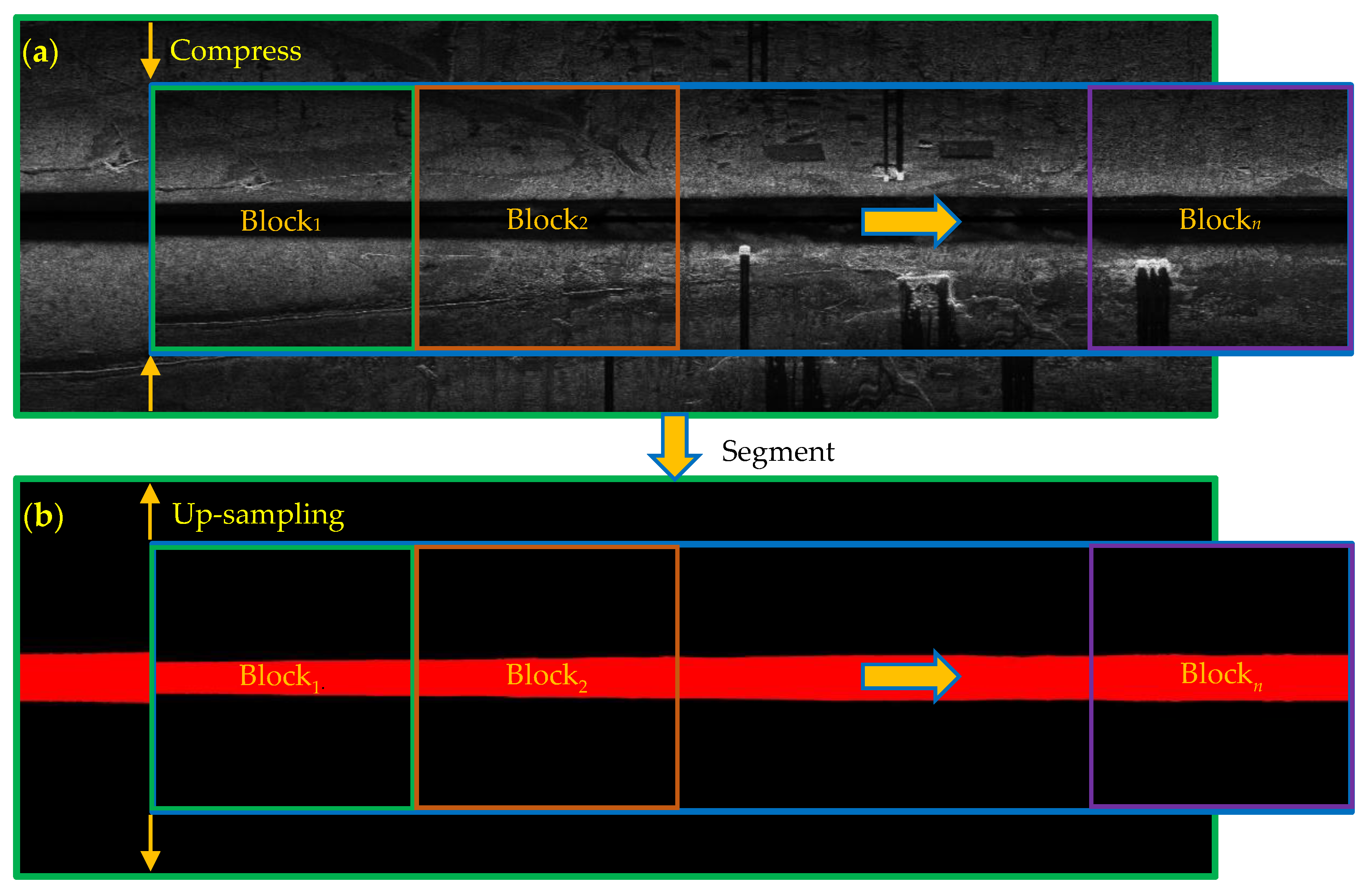
First, the raw SSS waterfall images are divided into blocks along the track. Each block has the same size as the training samples along the track. Then, each block is compressed to the same size as the training samples across the track and segmented separately. Next, the segmentation maps of each block are spliced together in order. Finally, the segmentation maps of the raw SSS waterfall images are obtained by up-sampling the stitched seg-mentation maps across the track.
2.3.2. Fast Bottom Line Search Method
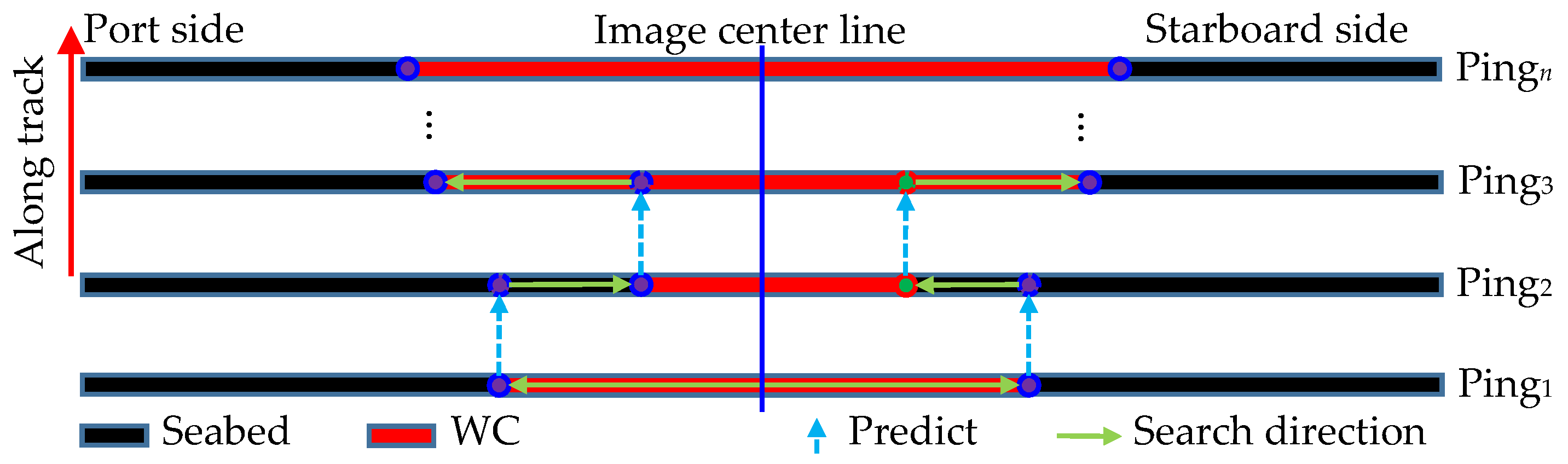
After the segmentation, the sea bottom lines composed of FBRs in successive pings can be extracted by searching the boundaries between the WC area and the seabed area. By traversing the segmented map from the middle to two sides across the track, the first echo classified as seabed is judged as the FBR. Once the FBR in current ping is found, the search is continued in the next ping. To reduce the number of traversal and improve the search speed, the positions of the FBRs in the previous ping are taken as the initial search position of the next ping in consideration of the continuity of the sea bottom line.
Considering the position relationship between the WC area and the seabed area in the SSS waterfall image, if the echo at the initial search position is classified as WC, the search direction is toward the corresponding image edge, otherwise toward the image center. The detailed search process is depicted in Figure 7.
2.3.3. Fine Segmentation to Improve Accuracy
Although the segmentation of high-resolution SSS waterfall images can be realized by the method described in Section 2.3.1, the segmentation errors will be enlarged because of the up-sampling operation. The relationship between bottom tracking error ΔBL and segmentation error ΔSeg is shown in Equation (4).
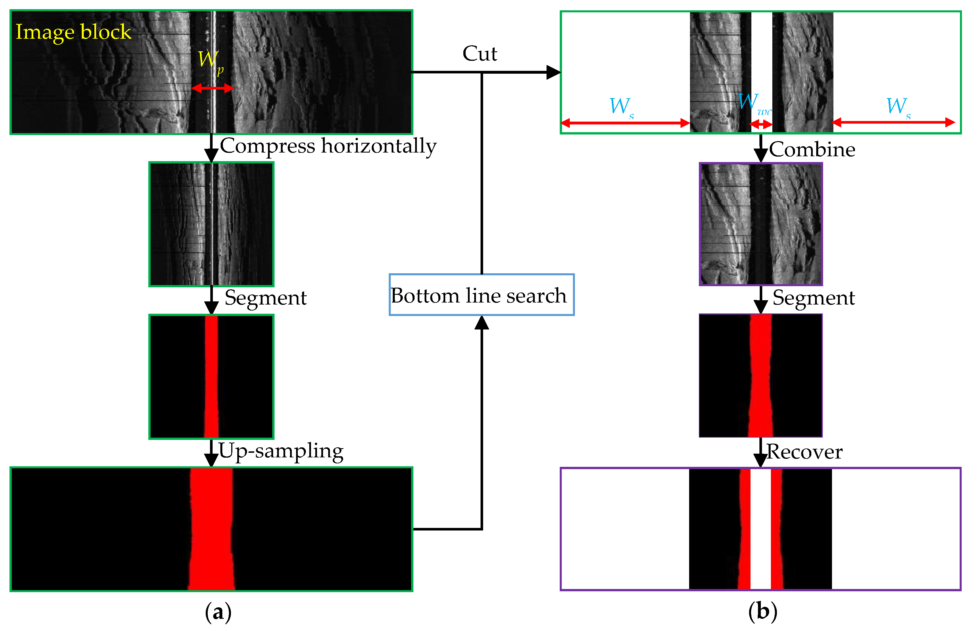
where N is the total number of samples in each ping, W is the width of the network output across the track. Assuming that the total number of samples per ping is 6000, the size of the input network image is 500 × 500, and the segmentation error is 1 pixel, then the sea bottom tracking error will be 6000/500 = 12 pixels, which is obviously intolerable. Therefore, an ingenious fine segmentation method is proposed to avoid this problem, as shown in Figure 8.
First, the coarse segmentation is performed on the waterfall image. Then, according to the bottom lines extracted from the coarse segmentation map, we can symmetrically remove part of seabed area and WC area in the image, and recombine the remaining image into a new image for fine segmentation with the same trained model. The width of the water column area and the seabed area removed Wwc, Ws can be calculated using the recommended Formulas (5) and (6).
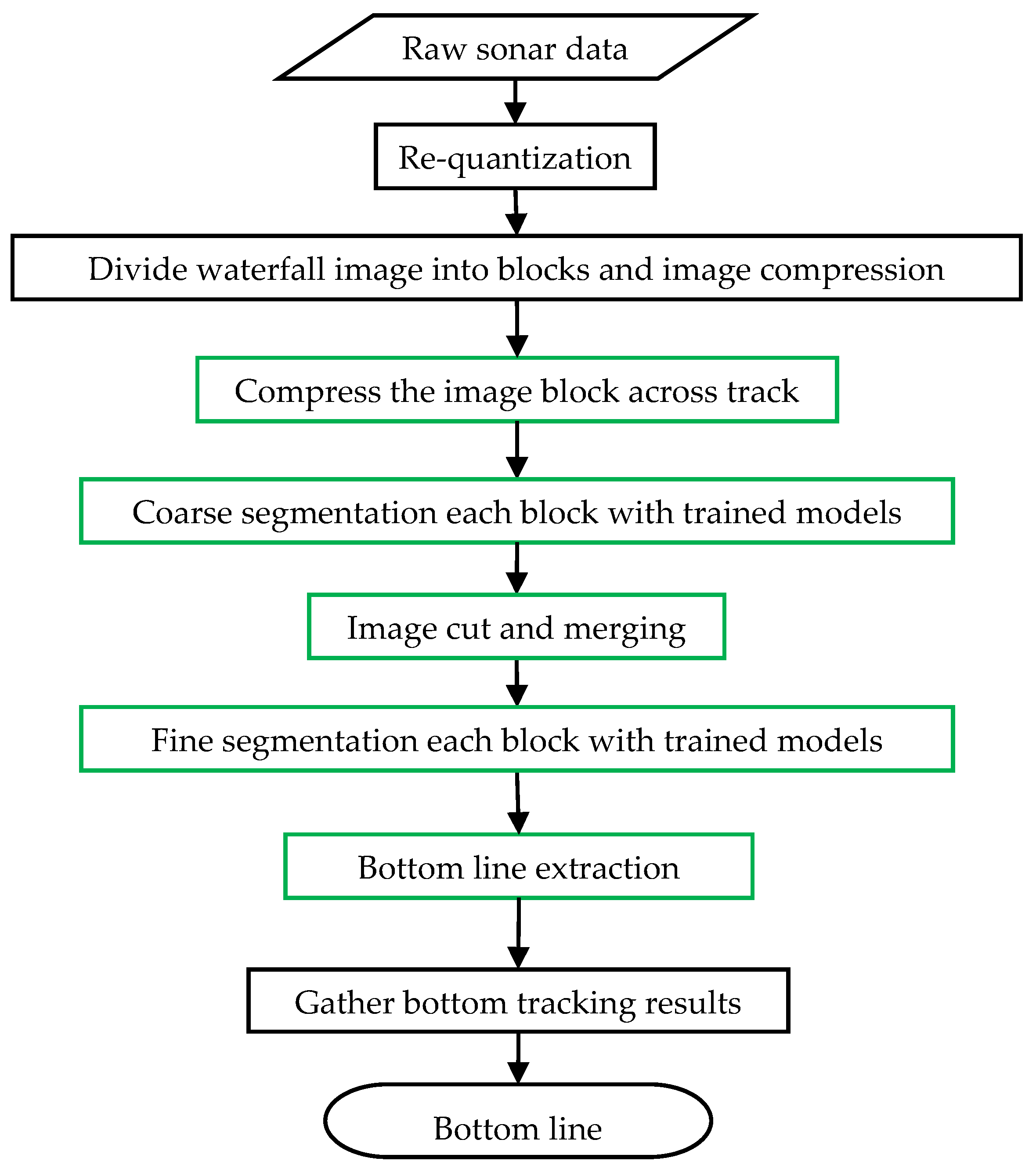
where N is the total number of samples in each ping, W is the width of the network output across the track, Wp is WC width of pings in the image block. More aggressive image removal strategies can also be adopted according to the requirement. Since the combined image will not be compressed or up-sampled when input into the network, the segmentation error will not be amplified when the segmentation map is recovered to the corresponding regions on the original waterfall image, and even the sub-pixel segmentation accuracy can be achieved when enough of the image is removed. The complete process of sea bottom tracking based on semantic segmentation is shown in Figure 9.
3. Experiment and Results
In order to verify the effectiveness of the proposed method, the raw data collected by various side-scan sonars (Klein3000, Klein 5000 V2, EdgeTech 4100P, EdgeTech 4125, EdgeTech 4200-MP, Benthos SIS-1624, DeepVision DE340, etc.) under different water environments (Yangtze River, Bohai Bay, Jiaozhou Bay, Beibu Gulf in China, Bay of Bengal, etc.) were selected for the experiment. During these measurements, the SSS altitudes varied from 3 m to 35 m. The original data was coded into eXtended Triton Format (*.xtf files) and echo signals were quantified as an 8-bit or 16-bit integer without gain information. Some of the experiment data are disturbed by the influencing factors described in Section 2.1.2. These data are highly representative and cover most complex situations, and the bottom lines are tracked by the proposed method on a desktop computer equipped with common hardware (CPU: i7-8700, GPU: GTX1070).
3.1. Training Network
Firstly, the backscatter strength sequences in the original record were decoded and quantized into 8-bit waterfall image following the method proposed in Section 2.2.1. Then, 5082 samples were collected by the operation described in Section 2.2.2 and the sample number was doubled with data augmentation by flip each sample across the track. Finally, the samples were randomly divided into the training set and the validation set at a ratio of 3:1, namely 7656 training samples and 2508 verification samples. Next, the model parameters pre-trained on Pascal VOC data set were transferred as the initial weights to speed up the convergence speed of the network and prevent over-fitting. After being processed by the SISM proposed in Section 2.2.3, the samples were input into the network for training. Finally, the semantic segmentation model was obtained by fine-tuning the pre-trained weights through repeated iterations.
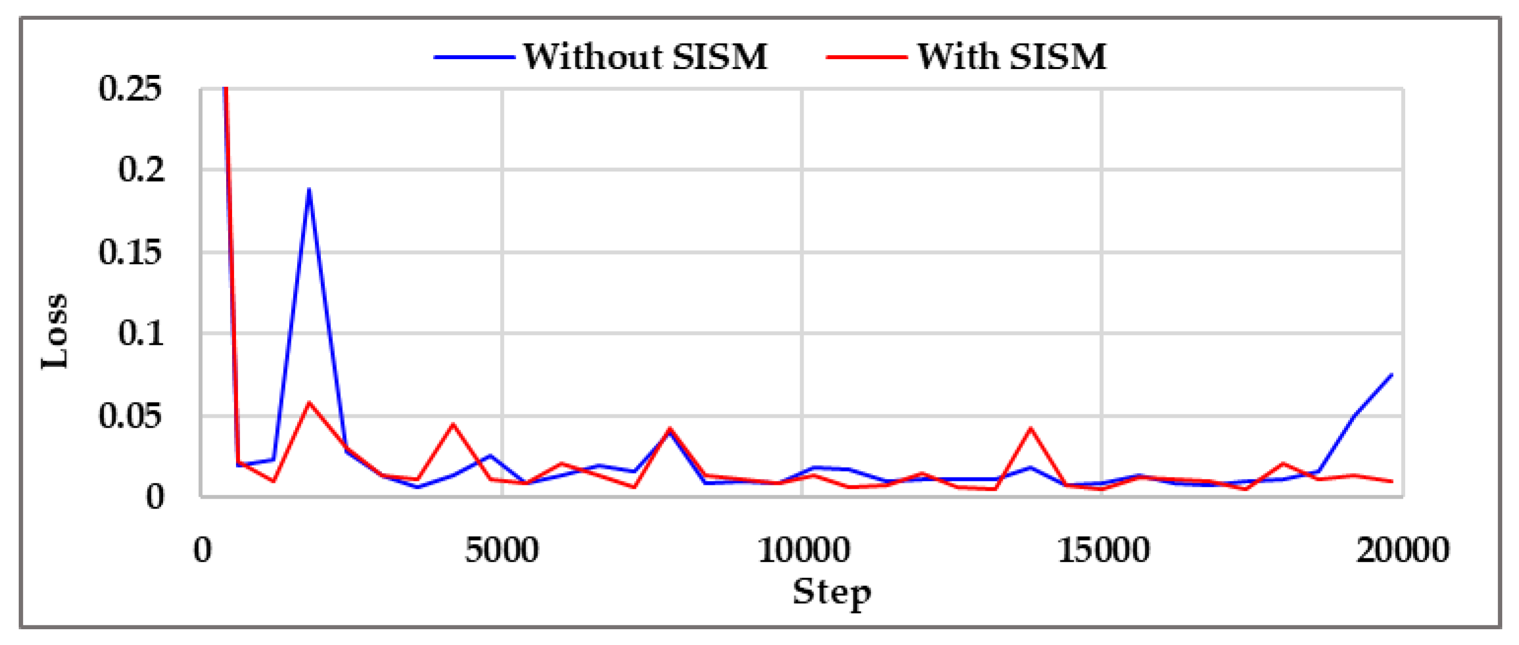
To verify the effectiveness of SISM, an ablation experiment was also conducted by directly training the network without SISM. It can be seen from Figure 10 that the loss values of both networks decrease gradually with the increase of training steps and become stable at 600th step. The fluctuation of the loss curve from the training process using the original network is more obvious than that using the network with SISM.
To further test the performances of the trained models, the trained models are used to segment the validation set. The segmentation accuracy is evaluated by MIoU (Mean Intersection over Union) [29]. The higher the MIoU is, the better the network performance is.
where i and j are label values of different categories, pij represents the number of pixels that belong to the i category but predicted as j category. pii represents the number of pixels correctly segmented, k is the maximum label value among all categories. The label value starts at 0, and k + 1 is the number of categories. For the segmentation of SSS image in this paper, k = 1, the pixels in the seabed area were labeled as 0 while in the WC area as 1. Ultimately, the MIoU of the model trained with the original network is 0.95 and the model trained with the network with SISM achieved a higher MIoU of 0.99, which means that the proposed SISM is helpful for improving the segmentation accuracy.
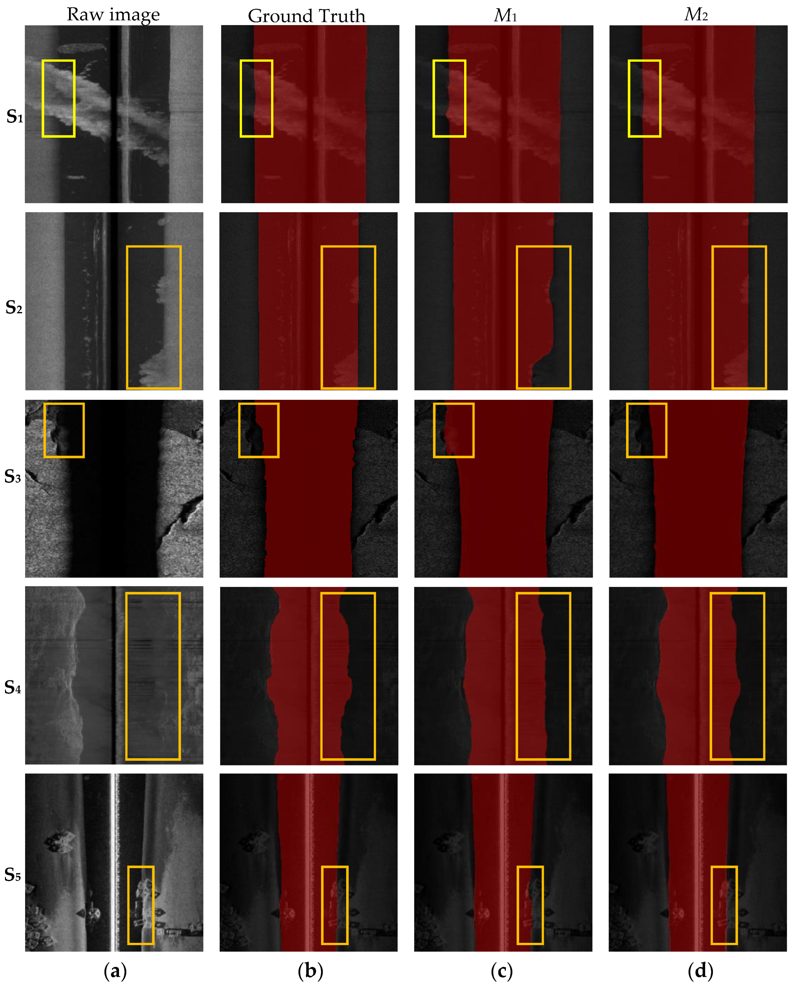
The segmentation results of some samples in the validation set are displayed in Figure 11, which shows the performance difference of two models. The segmentation results using the model trained with the original network (M1) and the network with SISM (M2) are shown in the third and fourth column, respectively.
In sample S1, the suspended solids cover the whole WC area, and the strong echo interference on the port side is more serious than the starboard side. It can be seen that both of the trained models can effectively segment the starboard image. Although the FBRs of some pings in the port image are completely submerged in the strong reflection, with the powerful context information acquisition ability of the network, M1 can still reasonably identify the WC area according to the distribution of the weak echoes in the surrounding pings. Moreover, because of the addition of SISM, more accurate segmentation results were achieved by M2.
In sample S2, the bottom line on the port image is very clear and the port WC area was recognized precisely by both models. However, the strong reflection in consecutive pings covers up portions of the bottom line on the starboard image, causing M1 to fail to segment the image correctly. Since M2 can comprehensively judge the echo information on both sides, it is still able to accurately segment the starboard image.
There are strong absorption sediments in sample S3, leading to low echo intensity in the seabed area and making it hard to distinguish the WC area from the seabed area near the boundary on the port image. The segmentation results of M2 are still significantly better than M1.
Sample S4 is severely disturbed by noises, causing the low contrast between the WC area and the seabed area. Besides, there are invalid pings in the image. It is almost impossible to determine the bottom line in the starboard image. M1 achieved good segmentation results at the port side, but cannot deal with the starboard image properly. While M2 intelligently inferred the WC range of the starboard image according to the WC area of the port image, and obtained reasonable segmentation results.
Sample S5 contains some artificial reefs, which brings difficulties for the traditional threshold methods to identify the true FBRs. However, both models have achieved fine results, and M2 is more excellent than M1 due to the integration of the port and starboard echo information.
The above comparisons show that M2 has better performance than M1 and can resist the influencing factors generally suffered in bottom tracking, which proves the effectiveness of the SISM proposed in this paper.
3.2. Bottom Tracking with Trained Model
In order to further verify the performance of the proposed method, the following experiments are carried out with several complete survey lines measured by various types of SSS in different water environments. Besides, the sea bottom tracking results are compared with the state-of-the-art method (hereafter referred to as CM) proposed in literature [17].
3.2.1. Sea Bottom Tracking Accuracy
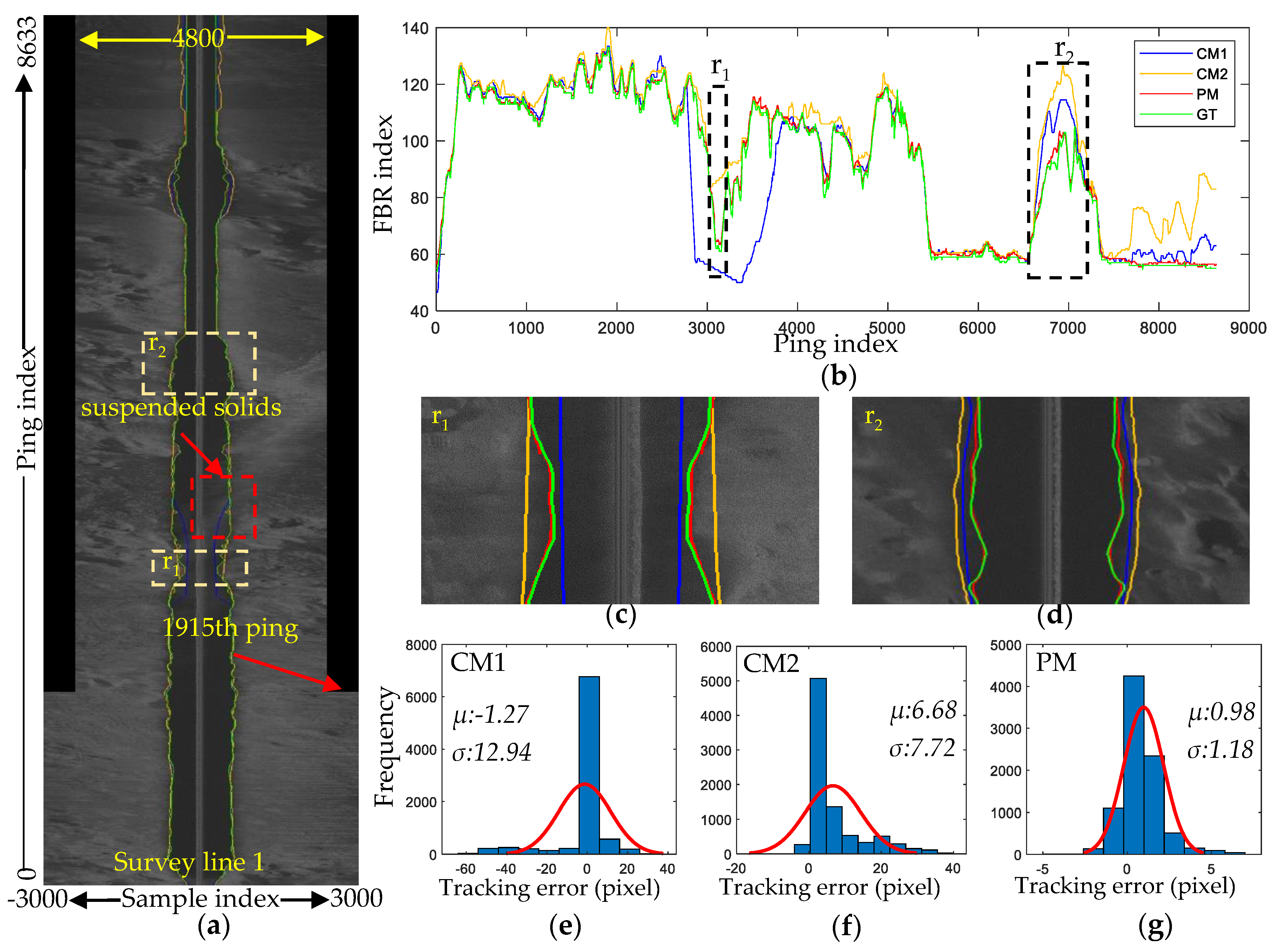
The waterfall image in Figure 12 was generated from the raw data measured by a Shark-S150D SSS with the operating frequency of 450 kHz in Pearl River Estuary, China with the re-quantization method described in Section 2.2.1. From the 1915th ping, the echo number per ping changed from 6000 to 4800 and the pixels without valid echoes were filled with zero. The whole image is disturbed by noise and the strong echoes from suspended solids in part of the WC area. The sedimentary facies at the nadir of the sonar varied greatly along the survey line and the tow-fish altitude also changed greatly.
The bottom lines were extracted following the steps described in Section 2.3. And the CM was also implemented for comparison. In the pings where echoes from the WC area and the seabed area have a high contrast, both methods can achieve satisfactory results comparable to the manual results. However, the CM required manual adjustment of the minimum altitude and gray difference thresholds to obtain better results, which is time consuming. Besides, although several sets of parameters were tried, the CM was still unable to achieve good tracking results among the whole survey line, as shown in Figure 12b. When the tow-fish heights change greatly, the constant parameter of minimum height will be less efficient for avoiding the strong echoes in a wider WC area. In addition, due to the existence of strong absorption sediments and suspended solids at the same time, it is difficult to find a suitable threshold to take into account both factors, as shown in Figure 12c and Figure 13d. In the pings disturbed by suspended solids, setting a small gray difference threshold will be not enough to avoid interference, while in pings with strong absorption sediments, a larger threshold will lead to larger tracking results. However, the method proposed in this paper (hereafter referred to as PM) achieved excellent bottom tracking results in the entire survey line, which proves its effectiveness and superiority.
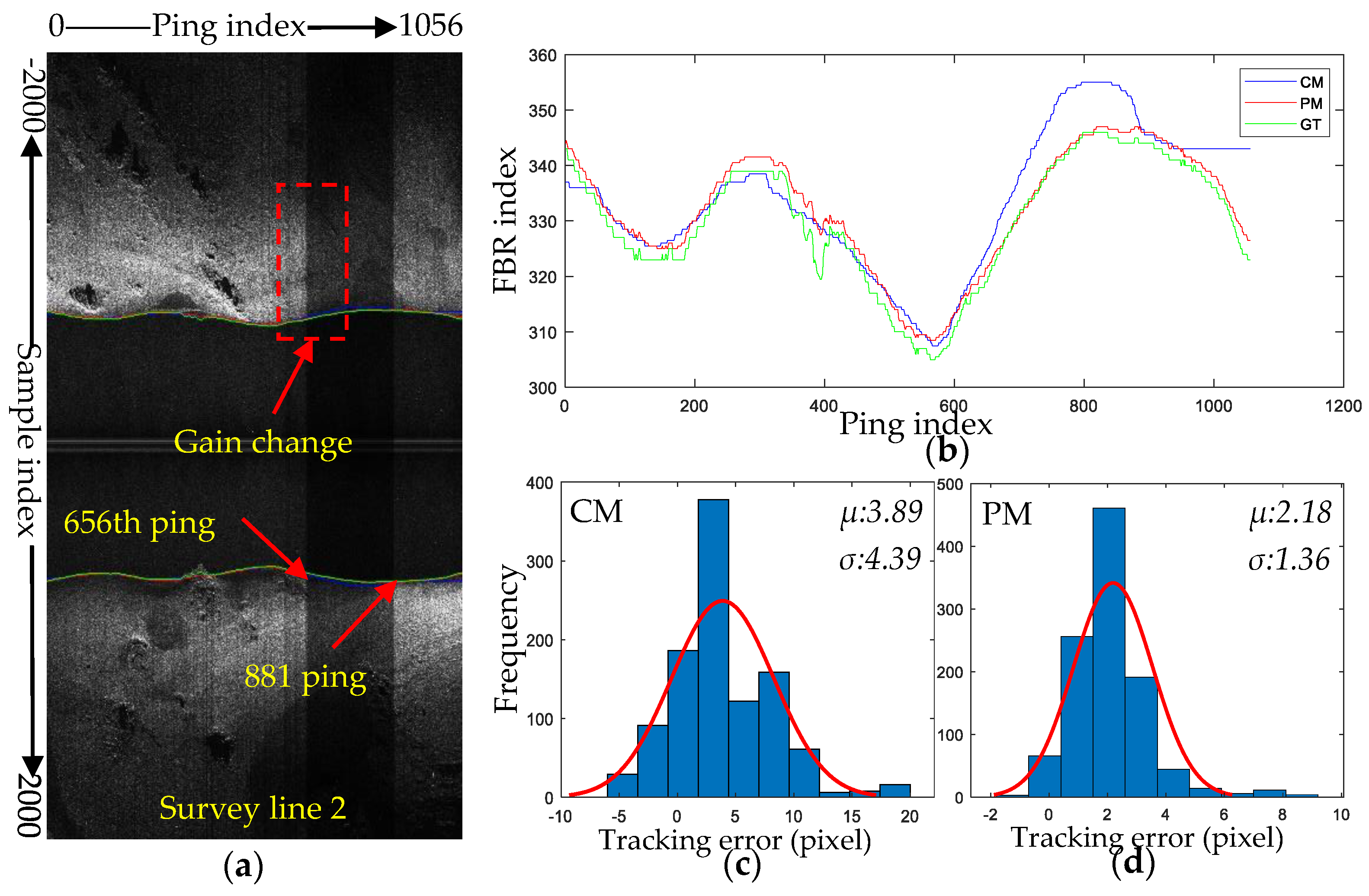
To test the ability of the proposed method to cope with the situation of unknown gains, the SSS data measured by EdgeTech4205 with an operating frequency of 41 Hz at Kyaukpyu, Myanmar were chosen for bottom tracking. The unknown gains changed at the 656th ping and 881th ping during the measurement, as shown in Figure 13a. In this case, the CM cannot adapt to the change due to fixed thresholds, which leads to the deviation of tracking results, as shown in Figure 13b. Thanks to the powerful pattern recognition capabilities of the neural networks, the proposed method could still identify the position of the bottom lines accurately.
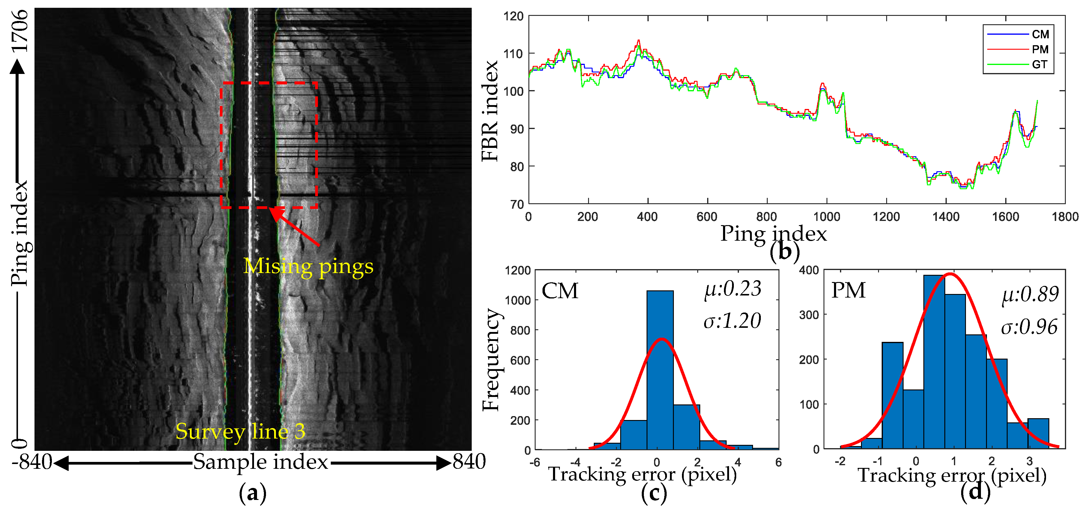
The SSS data in Figure 14. was collected by EdgeTech4100p at 500 kHz in Meizhou Bay, China. There are some missing pings in the waterfall image and the waterfall image is disturbed by strong echoes in the WC area. Since the CM considered the continuity and the symmetry of the bottom lines, by setting proper minimum altitude, gray difference threshold, and smoothing parameters, it achieved pretty good bottom tracking results. The proposed method can also take into account the symmetry of the bottom lines and it has strong context acquisition capability, therefore, the position of the FBRs in the missing pings can be reasonably inferred through adjacent pings and comparable results were obtained without any manual intervention.
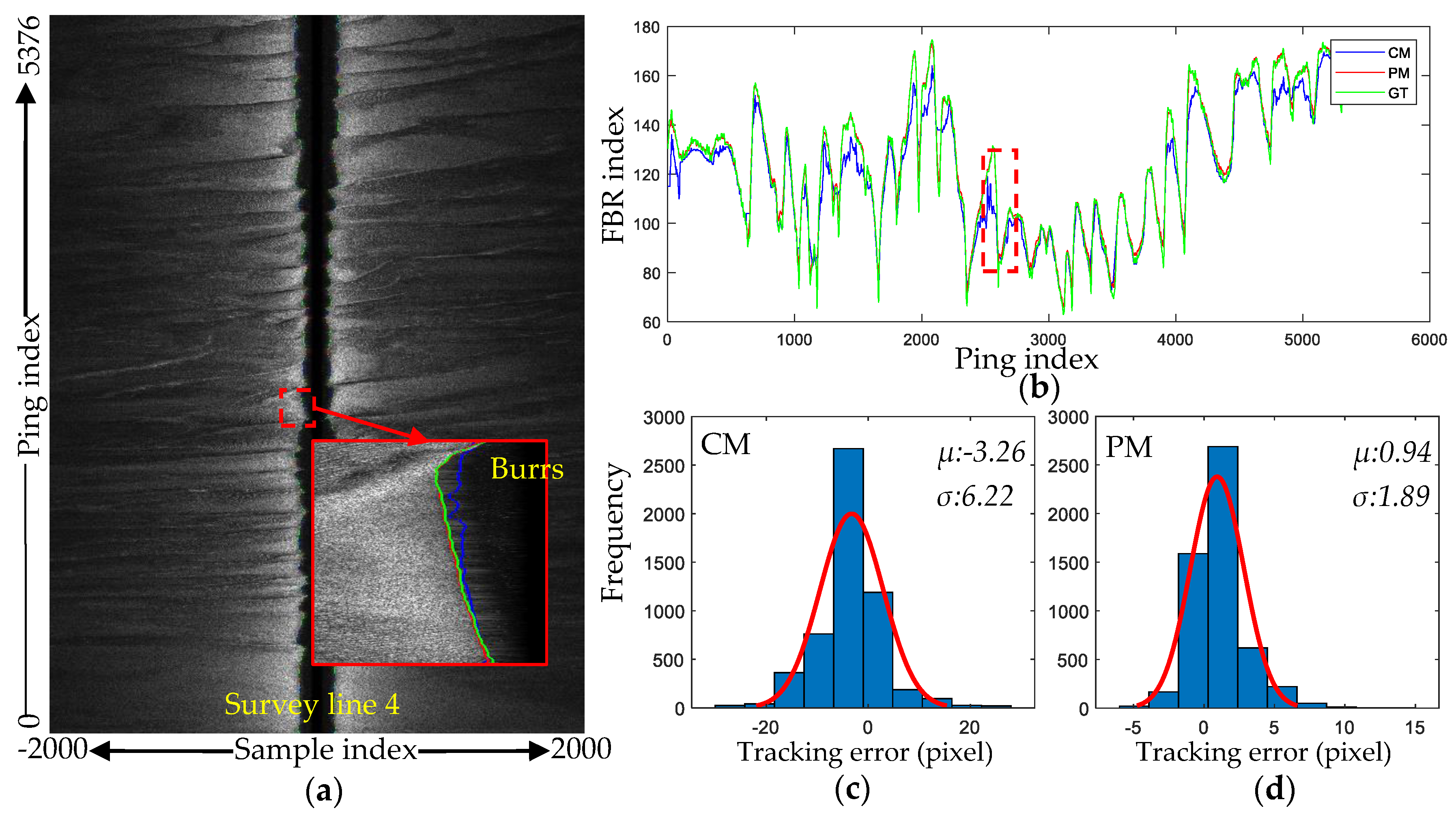
In order to verify the performance of the proposed method in dealing with special terrains, the SSS data measured by an unknown type of SSS at 122 kHz in Beibu Gulf, China was tested. Since there are a lot of sand waves in this area, the terrain at the nadir of SSS changes drastically, and there are many burrs around the bottom lines, as shown in Figure 15a. A minimum altitude parameter of 5.5 m and a gray difference of 24 was adopted by the CM when detecting the bottom lines. By comparing the tracking results, it can be seen that the proposed method is more consistent with the manual detection results than the CM.
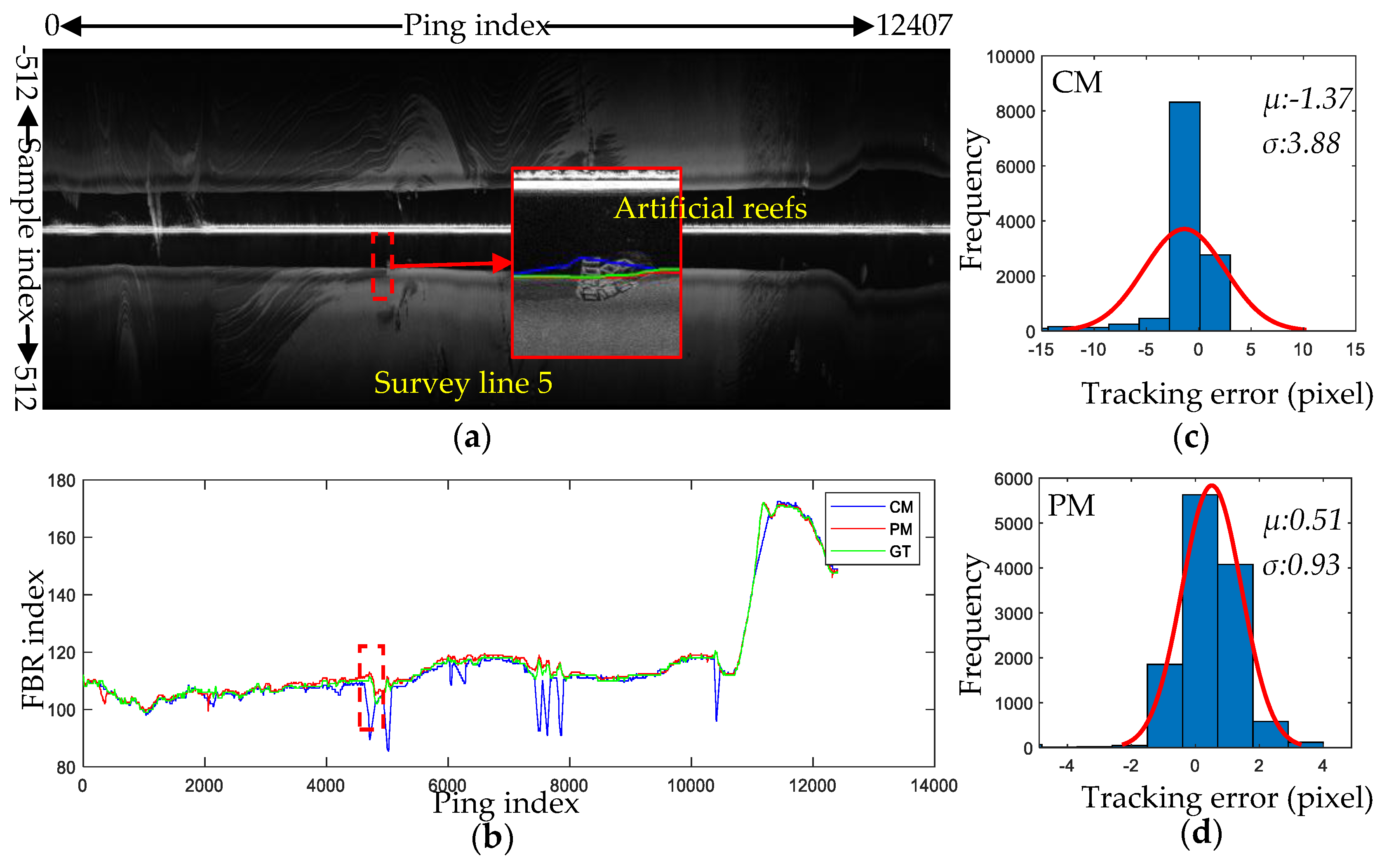
In order to perform more rigorous testing on the proposed method, a survey line data measured by DeepVision DE340 at 340 kHz in Xiangshan Bay, China was also tested, in which many artificial reefs were deployed on the seabed. Since the CM mainly judged the position of the FBR based on the gray-level difference of the adjacent sampling points in each ping, the strong echoes of the artificial reefs were mis-judged as the FBRs, as shown in Figure 16a. The proposed method can integrate the features of different scales and has a large receptive field. Therefore, it can avoid the false reflection signals of the artificial reefs and locate the real position of the bottom lines accurately.
The specific mean errors and standard deviations of the tracked bottom lines in the above experiments are listed in Table 1. Except for the mean error of line 3, the proposed method achieved better results than CM. The performance of CM was greatly affected by threshold parameters. However, the proposed method achieved high-precision bottom tracking results among all experiments without any manual intervention.
3.2.2. The Efficiency of the Proposed Method
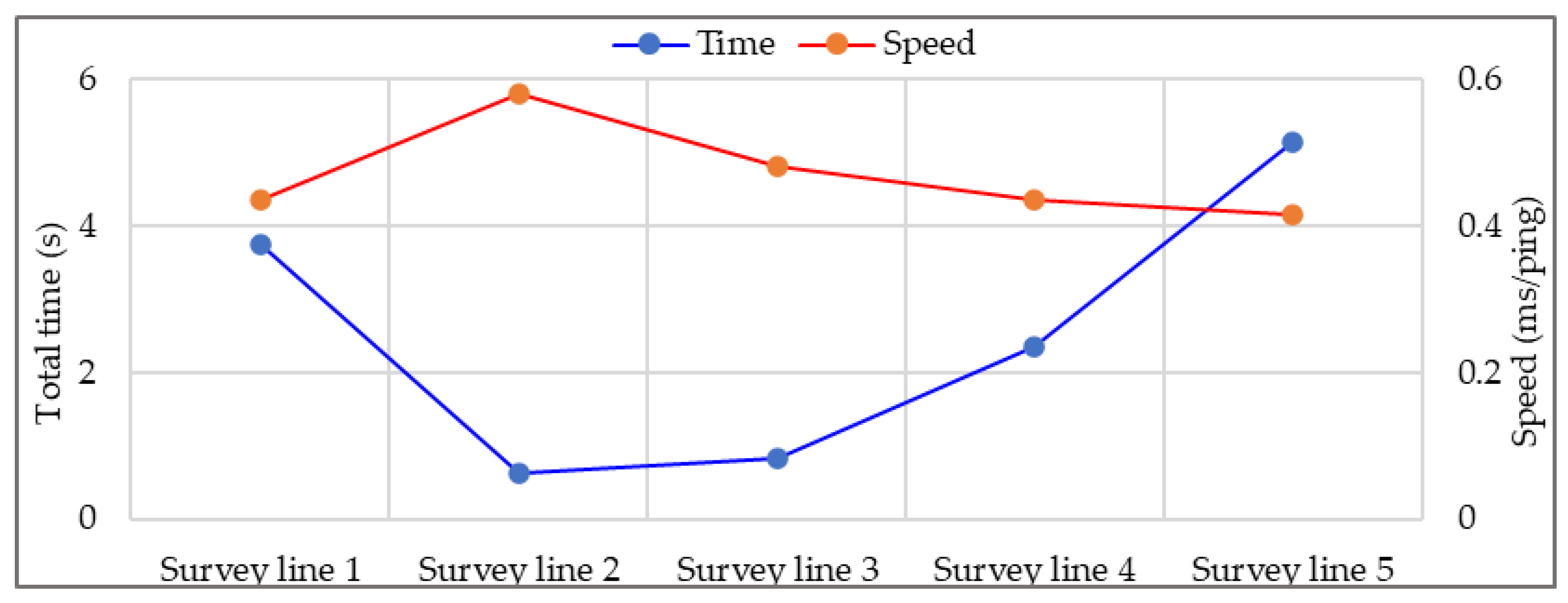
In order to evaluate the efficiency of the proposed method, the total bottom tracking time consumed by each survey line and the bottom tracking speed are calculated, as shown in Figure 17. The bottom tracking speed of the proposed method on the same desktop computer as the network training stage is about 0.47 ms/ping, that is 2128 ping/s, which is about 319 times faster than SSS ping sampling rate (Typically 150 ms/ping [21]). Because the Segmentation process of each image block was exactly the same without any manual intervention, and the fast bottom line search method almost took no time, the relationship between the time consumed and the number of pings is basically linear. However, CM needs to set the parameters manually, and requires adjusting the parameters repeatedly to get good results. Even in some complex situations, the results need to be optimized manually. The time spent is also related to the operator’s experience, and cannot be estimated accurately.
4. Discussion
4.1. Superiority Compared with the Traditional Methods
Traditional bottom tracking methods usually adopt simple local gray or gray difference features to detect the FBRs, so they are susceptible to interference from various influencing factors and often require a complicated optimization process. Compared with the traditional bottom tracking methods, our method is based on semantic segmentation network and the network used in the method has powerful multi-scale feature extraction capabilities, so it has strong anti-interference ability and high segmentation accuracy. In addition, in view of the symmetry of the sea bottom lines, the SISM ingeniously designed in this paper can not only weakens the strong echoes in the WC area, but also give the network the ability to synthesize the symmetrical position information of the both sides, which further improves the performance of the algorithm.
4.2. Efficiency Advantage
Our method achieved the fast bottom tracking of SSS data on a generic desktop personal computer, thus having high spreading value. There are three factors leading to the success:
- The proposed coarse-to-fine segmentation strategy makes the segmentation of each image block only need the network forward calculation twice. If the position of FBRs in each ping is located based on sequence recognition, a traversal process must be done along the echo sequence, which will require far more network calculations than the method proposed in this paper.
- Semantic segmentation network can share the calculation. Only one calculation is needed to get the features of all input pixels and determine their categories, which greatly improves the calculation efficiency. Since the sequences around the adjacent sampling have high similarity, the bottom tracking method based on sequence recognition will do a lot of repeated calculation, which wastes computing resources.
- The fast bottom line search method proposed in this paper almost took no time, which further improved the efficiency of the proposed bottom tracking method.
4.3. Real-Time Bottom Tracking
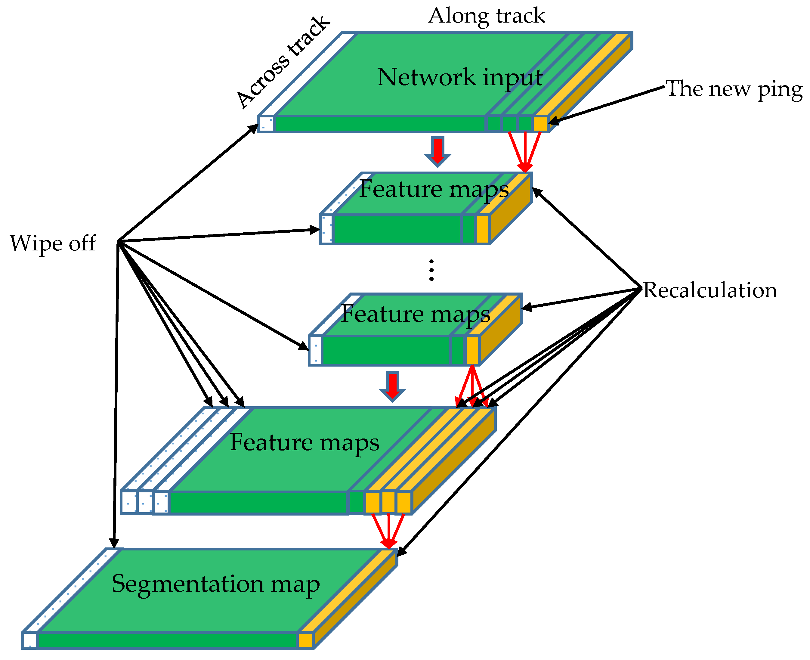
Although the average time spent per ping of the proposed method is short, the average processing speed of each image block (513 pings) is relatively slow, which is not enough for the real-time bottom tracking. In order to improve the real-time performance of the proposed method, there is an optimization idea that can be tried in the future as shown in Figure 18. The semantic segmentation network is a fully convolutional network (FCN), and the FCN does not include any fully connected layer, therefore, each activation value in the feature maps is only related to part of the layer’s input values. When a new ping comes, only part of the values is affected. We only need to recalculate the affected value, and clear the useless value, which not only ensures that the model remains unchanged, but also greatly reduces the computation, so as to meet the requirement of real-time bottom tracking.
4.4. Exceptional Situations
Although the proposed method has been verified with the data collected by different types of SSS in various complicated measuring environments, there are still some possible situations that might affect the result:
- The sonar is towed too close to the seafloor. In this case, the ratio of the width of the WC area to the seabed area will be too small, and the WC area may become very narrow due to the compression of the image during the coarse segmentation stage, resulting in segmentation errors, and then the fine segmentation cannot be carried out normally. This situation can be avoided by cutting part of the seabed image properly in advance.
- There are too many successive pings in which the water column area and seabed area are completely indistinguishable. Since our method implements the bottom tracking process with a patch-wise strategy, if the WC area of an image block is completely contaminated by the influencing factors summarized in Section 2.1.2, the network cannot obtain enough information to distinguish the WC area from the seabed area. This problem can be solved by interpolating the well-extracted bottom lines.
5. Conclusions
This paper proposes a robust bottom tracking method based on semantic segmentation. First, the waterfall images generated from raw SSS backscatter sequences are segmented by the well-trained DeepLabv3+ with the proposed SISM and a coarse-to-fine segmentation strategy is proposed to improve the segmentation accuracy. Then, the bottom line is located by the proposed fast search algorithm. The proposed method is verified by data measured by various devices in different underwater environments. The results show that the method is able to deal with various influencing factors in the SSS data, such as strong echoes in the WC area, low contrast, unknown gains, missing pings, etc. Moreover, the method achieved an average accuracy of 1.1 pixels of mean error and 1.26 pixels of standard deviation at the speed of 2128 ping/s, which is superior to existing bottom tracking algorithms. Most importantly, the process is completely automated without any manual intervention. The proposed method in this paper greatly improves the processing efficiency of SSS data and will further promote the application of SSS in underwater surveys.
Author Contributions
Conceptualization, G.Z. and H.Z.; methodology, G.Z.; software, G.Z.; validation, H.Z., Y.L. and J.Z.; formal analysis, H.Z.; investigation, G.Z. and Y.L.; resources, J.Z.; data curation, G.Z.; writing—original draft preparation, G.Z.; writing—review and editing, Y.L. and J.Z.; visualization, G.Z.; supervision, H.Z.; project administration, J.Z.; funding acquisition, H.Z. and J.Z. All authors have read and agreed to the published version of the manuscript.
Funding
This research was funded by National Natural Science Foundation of China under Grant 41576107 and Grant 41376109, in part by National Key R&D Program of China under Grant 2016YFB0501703.
Data Availability Statement
Access to the data will be considered upon request by the authors.
Acknowledgments
We would like to thank our colleagues for their helpful suggestions during the experiment, and thank the editor and the anonymous reviewers for their valuable comments and suggestions that greatly improve the quality of this paper.
Conflicts of Interest
The authors declare no conflict of interest.
References
- Acosta, G.G.; Villar, S.A. Accumulated CA-CFAR Process in 2-D for Online Object Detection from Sidescan Sonar Data. IEEE J. Ocean. Eng. 2015, 40, 558–569. [Google Scholar] [CrossRef]
- Mishne, G.; Talmon, R.; Cohen, I. Graph-Based Supervised Automatic Target Detection. IEEE Trans. Geosci. Remote 2015, 53, 2738–2754. [Google Scholar] [CrossRef]
- Rhinelander, J. Feature Extraction and Target Classification of Side-Scan Sonar Images. In Proceedings of the 2016 IEEE Symposium Series on Computational Intelligence (SSCI), Athens, Greece, 6–9 December 2016. [Google Scholar]
- Zheng, L.Y.; Tian, K. Detection of small objects in sidescan sonar images based on POHMT and Tsallis entropy. Signal Process. 2018, 142, 168–177. [Google Scholar] [CrossRef]
- Wang, X.; Zhao, J.H.; Zhu, B.Y.; Jiang, T.C.; Qin, T.T. A Side Scan Sonar Image Target Detection Algorithm Based on a Neutrosophic Set and Diffusion Maps. Remote Sens. 2018, 10, 295. [Google Scholar] [CrossRef] [Green Version]
- Feldens, P.; Darr, A.; Feldens, A.; Tauber, F. Detection of Boulders in Side Scan Sonar Mosaics by a Neural Network. Geosciences 2019, 9, 159. [Google Scholar] [CrossRef] [Green Version]
- Degraer, S.; Moerkerke, G.; Rabaut, M.; Van Hoey, G.; Du Four, I.; Vincx, M.; Henriet, J.P.; Van Lancker, V. Very-high resolution side-scan sonar mapping of biogenic reefs of the tube-worm Lanice conchilega. Remote Sens. Environ. 2008, 112, 3323–3328. [Google Scholar] [CrossRef]
- Van Overmeeren, R.; Craeymeersch, J.; van Dalfsen, J.; Fey, F.; van Heteren, S.; Meesters, E. Acoustic habitat and shellfish mapping and monitoring in shallow coastal water—Sidescan sonar experiences in The Netherlands. Estuar. Coast. Shelf Sci. 2009, 85, 437–448. [Google Scholar] [CrossRef]
- Nguyen, H.T.; Lee, E.H.; Lee, S. Study on the Classification Performance of Underwater Sonar Image Classification Based on Convolutional Neural Networks for Detecting a Submerged Human Body. Sensors 2020, 20, 94. [Google Scholar] [CrossRef] [Green Version]
- Brown, C.J.; Smith, S.J.; Lawton, P.; Anderson, J.T. Benthic habitat mapping: A review of progress towards improved understanding of the spatial ecology of the seafloor using acoustic techniques. Estuar. Coast. Shelf Sci. 2011, 92, 502–520. [Google Scholar] [CrossRef]
- Switzer, T.S.; Tyler-Jedlund, A.J.; Keenan, S.F.; Weather, E.J. Benthic Habitats, as Derived from Classification of Side-Scan-Sonar Mapping Data, Are Important Determinants of Reef-Fish Assemblage Structure in the Eastern Gulf of Mexico. Mar. Coast Fish. 2020, 12, 21–32. [Google Scholar] [CrossRef]
- Buscombe, D. Shallow water benthic imaging and substrate characterization using recreational-grade sidescan-sonar. Environ. Modell. Softw. 2017, 89, 1–18. [Google Scholar] [CrossRef] [Green Version]
- Shang, X.; Zhao, J.; Zhang, H. Automatic Overlapping Area Determination and Segmentation for Multiple Side Scan Sonar Images Mosaic. IEEE J. Select. Top. Appl. Earth Obs. Remote Sens. 2021, 14, 2886–2900. [Google Scholar] [CrossRef]
- Blondel, P. The Handbook of Sidescan Sonar; Praxis Publishing Ltd.: Chichester, UK, 2009; p. 65. [Google Scholar]
- Discover 4200 Users Software Manual. Available online: https://www.edgetech.com/wp-content/uploads/2019/07/0004841_Rev_C.pdf (accessed on 21 March 2020).
- Woock, P. Side-scan sonar based SLAM for the deep sea. In Proceedings of the Joint Workshop of Fraunhofer IOSB and Institute for Anthropomatics, Vision and Fusion Laboratory, La Bresse, France, 19–23 July 2010. [Google Scholar]
- Zhao, J.H.; Wang, X.; Zhang, H.M.; Wang, A.X. A Comprehensive Bottom-Tracking Method for Sidescan Sonar Image Influenced by Complicated Measuring Environment. IEEE J. Ocean. Eng. 2017, 42, 619–631. [Google Scholar] [CrossRef]
- Al-Rawi, M.; Elmgren, F.; Frasheri, M.; Çürüklü, B.; Yuan, X.; Martínez, J.-F.; Bastos, J.; Rodriguez, J.; Pinto, M. Algorithms for the Detection of First Bottom Returns and Objects in the Water Column in Sidescan Sonar Images. In Proceedings of the OCEANS 2017, Aberdeen, Aberdeen, UK, 19–22 June 2018. [Google Scholar]
- Shih, C.C.; Horng, M.F.; Tseng, Y.R.; Su, C.F.; Chen, C.Y. An Adaptive Bottom Tracking Algorithm for Side-Scan Sonar Seabed Mapping. In Proceedings of the 2019 IEEE Underwater Technology (UT), Kaohsiung, Taiwan, 16–19 April 2019. [Google Scholar]
- Wang, A.X.; Church, I.; Gou, J.; Zhao, J.H. Sea bottom line tracking in side-scan sonar image through the combination of points density clustering and chains seeking. J. Mar. Sci. Technol.-Jpn. 2020, 25, 849–865. [Google Scholar] [CrossRef]
- Yan, J.; Meng, J.X.; Zhao, J.H. Real-Time Bottom Tracking Using Side Scan Sonar Data through One-Dimensional Convolutional Neural Networks. Remote Sens. 2020, 12, 37. [Google Scholar] [CrossRef] [Green Version]
- Lin, G.S.; Milan, A.; Shen, C.H.; Reid, I. RefineNet: Multi-Path Refinement Networks for High-Resolution Semantic Segmentation. In Proceedings of the IEEE Conference on Computer Vision and Pattern Recognition (CVPR), Honolulu, HI, USA, 21–26 July 2017. [Google Scholar]
- Hu, J.; Shen, L.; Albanie, S.; Sun, G.; Wu, E.H. Squeeze-and-Excitation Networks. IEEE Trans. Pattern Anal. 2020, 42, 2011–2023. [Google Scholar] [CrossRef] [Green Version]
- Bochkovskiy, A.; Wang, C.-Y.; Liao, H.-Y. YOLOv4: Optimal Speed and Accuracy of Object Detection. arXiv 2020, arXiv:2004.10934. [Google Scholar]
- Zhu, P.P.; Isaacs, J.; Fu, B.; Ferrari, S. Deep Learning Feature Extraction for Target Recognition and Classification in Underwater Sonar Images. In Proceedings of the 2017 IEEE 56th Annual Conference on Decision and Control (CDC), Melbourne, Australia, 12–15 December 2017. [Google Scholar]
- Li, C.L.; Ye, X.F.; Cao, D.X.; Hou, J.; Yang, H.B. Zero shot objects classification method of side scan sonar image based on synthesis of pseudo samples. Appl. Acoust. 2021, 173, 107691. [Google Scholar] [CrossRef]
- Huo, G.Y.; Wu, Z.Y.; Li, J.B. Underwater Object Classification in Sidescan Sonar Images Using Deep Transfer Learning and Semisynthetic Training Data. IEEE Access 2020, 8, 47407–47418. [Google Scholar] [CrossRef]
- Song, Y.; He, B.; Liu, P.; Yan, T.H. Side scan sonar image segmentation and synthesis based on extreme learning machine. Appl. Acoust. 2019, 146, 56–65. [Google Scholar] [CrossRef]
- Wang, Q.; Wu, M.H.; Yu, F.; Feng, C.; Li, K.G.; Zhu, Y.M.; Rigall, E.; He, B. RT-Seg: A Real-Time Semantic Segmentation Network for Side-Scan Sonar Images. Sensors 2019, 19, 1985. [Google Scholar] [CrossRef] [Green Version]
- Lurton, X. An Introduction to Underwater Acoustics: Principles and Applications, 2nd ed.; Springer: New York, NY, USA, 2011; p. 336. [Google Scholar]
- Goodfellow, I.; Bengio, Y.; Courville, A. Deep Learning; MIT Press: Cambridge, MA, USA, 2016; pp. 326–333. [Google Scholar]
- Chen, L.C.E.; Zhu, Y.K.; Papandreou, G.; Schroff, F.; Adam, H. Encoder-Decoder with Atrous Separable Convolution for Semantic Image Segmentation. In Proceedings of the European Conference on Computer Vision (ECCV), Munich, Germany, 8–14 September 2018. [Google Scholar]
- Ronneberger, O.; Fischer, P.; Brox, T. U-Net: Convolutional Networks for Biomedical Image Segmentation. Lect. Notes Comput. Sci. 2015, 9351, 234–241. [Google Scholar]
- Zhao, H.S.; Shi, J.P.; Qi, X.J.; Wang, X.G.; Jia, J.Y. Pyramid Scene Parsing Network. In Proceedings of the IEEE Conference on Computer Vision and Pattern Recognition (CVPR), Honolulu, HI, USA, 21–26 July 2017. [Google Scholar]
Figure 1.
Working principle of SSS. (a) shows the imaging principle of SSS. (b) shows a typical SSS waterfall image.
Figure 1.
Working principle of SSS. (a) shows the imaging principle of SSS. (b) shows a typical SSS waterfall image.

Figure 2.
Influencing factors of FBR detection in SSS data. (a,b) Suspended solids. (c) Ship wake. (d) Sound reflection from sea surface. (e) Water with high turbidity. (f) Strong absorption sediments. (g) Varying gains. (h) Missing pings.
Figure 2.
Influencing factors of FBR detection in SSS data. (a,b) Suspended solids. (c) Ship wake. (d) Sound reflection from sea surface. (e) Water with high turbidity. (f) Strong absorption sediments. (g) Varying gains. (h) Missing pings.

Figure 3.
The process of collecting samples. (a) Waterfall image of a survey line. (b) Samples for training. ①~③ are three sub image blocks with different width.
Figure 3.
The process of collecting samples. (a) Waterfall image of a survey line. (b) Samples for training. ①~③ are three sub image blocks with different width.

Figure 4.
The well-designed symmetrical information synthesis module (SISM).

Figure 5.
Complete semantic segmentation network structure. The proposed SISM is add to the head of the network. The encoder module encodes multi-scale contextual information by applying atrous convolution at multiple scales, while the decoder module refines the segmentation results along object boundaries.

Figure 6.
The segmentation process of high-resolution side-scan sonar waterfall image. (a) Raw waterfall image. (b) Segmentation map.
Figure 6.
The segmentation process of high-resolution side-scan sonar waterfall image. (a) Raw waterfall image. (b) Segmentation map.

Figure 7.
Sea bottom line extraction process.

Figure 8.
Method to improve the accuracy of sea bottom tracking. (a) Coarse segmentation. (b) Fine segmentation.
Figure 8.
Method to improve the accuracy of sea bottom tracking. (a) Coarse segmentation. (b) Fine segmentation.

Figure 9.
Flowchart of the bottom tracking method based on semantic segmentation.

Figure 10.
Training loss of different networks.

Figure 11.
Segmentation performances of different trained models. (a) Original SSS image blocks with a size of 513 × 513 pixels. (b) Ground truth by manual labeling. (c) Segmentation results with M1. (d) Segmentation results with M2.
Figure 11.
Segmentation performances of different trained models. (a) Original SSS image blocks with a size of 513 × 513 pixels. (b) Ground truth by manual labeling. (c) Segmentation results with M1. (d) Segmentation results with M2.

Figure 12.
Bottom tracking experiment on the SSS data suffering from strong echoes in the WC area and low contrast between the WC area and seabed area. (a) Waterfall image re-quantized from raw SSS data. (b) Averaged bottom tracking results of port and starboard with the two methods. (c,d) are the bottom tracking results in region r1 and r2 respectively when applying different thresholds with the CM. (CM1: a minimum depth parameter of 4.0 m and a gray difference parameter of 8. CM2: 4.2 m, 15). (e–g) display the error distributions of CM1, CM2 and PM relative to the manual interpretation.

Figure 13.
Bottom tracking experiment on the SSS data applied with varying unknown gains. (a) Waterfall image re-quantized from raw SSS data. (b) Averaged bottom tracking results of port and starboard with the tow methods. (c,d) Error distribution relative to the manual interpretation.
Figure 13.
Bottom tracking experiment on the SSS data applied with varying unknown gains. (a) Waterfall image re-quantized from raw SSS data. (b) Averaged bottom tracking results of port and starboard with the tow methods. (c,d) Error distribution relative to the manual interpretation.

Figure 14.
Bottom tracking experiment on the SSS data with missing pings. (a) Waterfall image re-quantized from raw SSS data. (b) Averaged bottom tracking results of port and starboard with the tow methods. (c,d) Error distribution relative to the manual interpretation.
Figure 14.
Bottom tracking experiment on the SSS data with missing pings. (a) Waterfall image re-quantized from raw SSS data. (b) Averaged bottom tracking results of port and starboard with the tow methods. (c,d) Error distribution relative to the manual interpretation.

Figure 15.
Bottom tracking experiment on the SSS data with drastically changing terrain. (a) Waterfall image re-quantized from raw SSS data. (b) Averaged bottom tracking results of port and starboard with the tow methods. (c,d) Error distribution relative to the manual interpretation.
Figure 15.
Bottom tracking experiment on the SSS data with drastically changing terrain. (a) Waterfall image re-quantized from raw SSS data. (b) Averaged bottom tracking results of port and starboard with the tow methods. (c,d) Error distribution relative to the manual interpretation.

Figure 16.
Bottom tracking experiment on the SSS data with artificial architecture. (a) Waterfall image re-quantized from raw SSS data. (b) Averaged bottom tracking results of port and starboard with the tow methods. (c,d) Error distribution relative to the manual interpretation.
Figure 16.
Bottom tracking experiment on the SSS data with artificial architecture. (a) Waterfall image re-quantized from raw SSS data. (b) Averaged bottom tracking results of port and starboard with the tow methods. (c,d) Error distribution relative to the manual interpretation.

Figure 17.
Total time spent on each survey line and the corresponding bottom tracking speed.

Figure 18.
The schematic diagram of real-time tracking based on the PM.


Table 1.
Precision statistics of the bottom tracking results among the above tested data.
| Survey Line Number | Mean Error (Pixels) | STD (Pixels) | ||
|---|---|---|---|---|
| CM | PM | CM | PM | |
| 1 | −1.27 | 0.98 | 12.94 | 1.18 |
| 2 | 3.89 | 2.18 | 4.39 | 1.36 |
| 3 | 0.23 | 0.89 | 1.20 | 0.96 |
| 4 | −3.26 | 0.94 | 6.22 | 1.89 |
| 5 | −1.37 | 0.51 | 3.88 | 0.93 |
| Mean Absolute value | 2.00 | 1.1 | 5.73 | 1.26 |
Publisher’s Note: MDPI stays neutral with regard to jurisdictional claims in published maps and institutional affiliations. |
© 2021 by the authors. Licensee MDPI, Basel, Switzerland. This article is an open access article distributed under the terms and conditions of the Creative Commons Attribution (CC BY) license (https://creativecommons.org/licenses/by/4.0/).
Share and Cite
MDPI and ACS Style
Zheng, G.; Zhang, H.; Li, Y.; Zhao, J. A Universal Automatic Bottom Tracking Method of Side Scan Sonar Data Based on Semantic Segmentation. Remote Sens. 2021, 13, 1945. https://0-doi-org.brum.beds.ac.uk/10.3390/rs13101945
AMA Style
Zheng G, Zhang H, Li Y, Zhao J. A Universal Automatic Bottom Tracking Method of Side Scan Sonar Data Based on Semantic Segmentation. Remote Sensing. 2021; 13(10):1945. https://0-doi-org.brum.beds.ac.uk/10.3390/rs13101945
Chicago/Turabian StyleZheng, Gen, Hongmei Zhang, Yuqing Li, and Jianhu Zhao. 2021. "A Universal Automatic Bottom Tracking Method of Side Scan Sonar Data Based on Semantic Segmentation" Remote Sensing 13, no. 10: 1945. https://0-doi-org.brum.beds.ac.uk/10.3390/rs13101945
Note that from the first issue of 2016, this journal uses article numbers instead of page numbers. See further details here.