
Fast Target Localization Method for FMCW MIMO Radar via VDSR Neural Network


1
State Key Laboratory of Marine Resource Utilization in South China Sea, School of Information and Communication Engineering, Hainan University, Haikou 570228, China
2
Key Laboratory for Ubiquitous Network and Service Software of Liaoning Province, School of Software, Dalian University of Technology, Dalian 116620, China
*
Author to whom correspondence should be addressed.
Remote Sens. 2021, 13(10), 1956; https://0-doi-org.brum.beds.ac.uk/10.3390/rs13101956
Submission received: 29 March 2021
/
Revised: 10 May 2021
/
Accepted: 11 May 2021
/
Published: 17 May 2021
(This article belongs to the Special Issue Radar Signal Processing for Target Tracking)
Abstract
:The traditional frequency-modulated continuous wave (FMCW) multiple-input multiple-output (MIMO) radar two-dimensional (2D) super-resolution (SR) estimation algorithm for target localization has high computational complexity, which runs counter to the increasing demand for real-time radar imaging. In this paper, a fast joint direction-of-arrival (DOA) and range estimation framework for target localization is proposed; it utilizes a very deep super-resolution (VDSR) neural network (NN) framework to accelerate the imaging process while ensuring estimation accuracy. Firstly, we propose a fast low-resolution imaging algorithm based on the Nystrom method. The approximate signal subspace matrix is obtained from partial data, and low-resolution imaging is performed on a low-density grid. Then, the bicubic interpolation algorithm is used to expand the low-resolution image to the desired dimensions. Next, the deep SR network is used to obtain the high-resolution image, and the final joint DOA and range estimation is achieved based on the reconstructed image. Simulations and experiments were carried out to validate the computational efficiency and effectiveness of the proposed framework.
1. Introduction
Frequency-modulated continuous wave (FMCW) has achieved great success in the field of communications and has broad prospects in applications such as altimeters [1], vehicle radars [2,3,4] and synthetic aperture radars (SARs) [5,6,7,8,9]. The merits of FMCW radars lie in their ranging ability and low power consumption [10,11]. Recently, the FMCW multiple-input multiple-output (MIMO) radar was investigated, and it has an equivalent virtual antenna array, which independently pairs transmitting and receiving elements as virtual elements [12,13,14]. This greatly expands the aperture of the array, but is accompanied by a sharp increase in data dimensions. Moreover, the received signal of FMCW MIMO radar contains the information of direction-of-arrival (DOA) and range, which can be used for target localization. It is indicated that the resolution of range is proportional to the number of snapshots, which leads to a greatly reduced real-time performance of the system when expanding the dimensions of the data for target localization using traditional algorithms.
In order to achieve high accuracy target localization, joint DOA and range estimation with high resolution is the key issue. As solutions to joint DOA and range estimation, 2D algorithms have been proposed [13,15,16]. The 2D Fast Fourier Transformation (2D-FFT), which is a fast algorithm, is used to estimate DOA and range. Unfortunately, due to the limitations of the Rayleigh criterion and the bandwidth of FMCW MIMO systems, the resolution is not satisfactory. In order to improve the resolution, a 2D multiple signal classification (2D-MUSIC) algorithm for the joint angle and range estimation was presented, which was able to achieve good performance in the experimental data scenarios. However, as for the algorithm in [16], a huge covariance matrix and 2D spectral peak search are needed, which lead to high computational complexity. Thus, these methods make it difficult to meet the real-time requirements.
In recent years, with the rapid development of machine learning, super-resolution methods based on deep learning have become a hot spot [17], and the performances of these methods have come to significantly surpass those of common methods [18,19,20,21]. In [18], an SR algorithm based on sparse dictionary and anchored neighborhood regression (ANR) was proposed. It has superior reconstruction speed and quality. However, the anchored neighborhood projections of ANR are unstable for covering varieties of mapping relationships, so is not suitable for dealing with practical engineering problems. In [19], an image SR algorithm based on local linear regression and random forests was proposed. The stability of this method is higher than the method in [18], but it cannot deal with SR tasks with different magnifications either. In [20], an improved self-similarity based SR algorithm was proposed, which exploits the statistical prior of the same image. However, the internal dictionary is not always suitable, which leads to performance loss. In [21], a convolutional neural network (CNN) was firstly used to implement image SR. Although this method has excellent results due to its shallow network depth, it cannot achieve sufficient field of vision, and cannot support multiple high-definition. As a result, this method is difficult to use in SR tasks involving radar images with multiple sizes and grids. The emergence of very deep super resolution (VDSR) [17] was a qualitative leap for networks based on a pure CNN architecture. Whether it is an ultra-deep network structure or flexible image magnification, VDSR is more suitable for dealing with the problem of radar image super-resolution. This approach focuses on the brightness channel information of the image, reconstructs the brightness residual between the high-resolution image and the low-resolution image and finally obtains the high-resolution image. It is worth noting that the radar image can be regarded as a color image with only the brightness channel; thus, the VDSR framework is a more suitable representation of the reconstructed radar image.
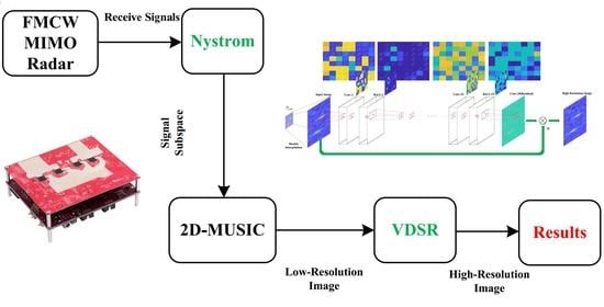
In this paper, we propose a fast joint DOA and range estimation framework based on a VDSR neural network to accelerate the estimation process without precision loss. The proposed framework splits the estimation process into two parts: In the first part, to solve the problem that the traditional 2D-MUSIC algorithm incurs a high computational cost during covariance decomposition, the Nystrom method [22] is introduced to use the covariance of partial data and obtain an approximate signal subspace. This procedure avoids the calculation of the original covariance matrix. Then, a low-density grid is used to generate small size and low-resolution images to avoid a massive 2D peak search. The second part focuses on improving the estimation accuracy of the whole framework. The VDSR network is used to construct a high-resolution image from the low-resolution image achieved in the first part. Finally, the DOA and range are estimated from peaks of the reconstructed image. The simulation results show that the proposed algorithm is much faster than the traditional high precision solutions and the experimental results further verify its performance.
The main contributions of our work are summarized as follows:
(1) A fast joint DOA and range estimation framework based on a VDSR neural network is proposed. The framework can estimate the DOA and the range of FMCW MIMO radar in a computationally efficient manner without precision loss.
(2) The proposed framework uses the Nystrom method to reduce the computational complexity of the high-dimensional matrix signal subspace, and VDSR to ensure the accuracy of the estimation.
(3) Simulations and experiments were carried out to validate the proposed framework, and it is demonstrated that running time is greatly reduced without loss of accuracy.
The rest of the paper is organized as follows. In Section 2, the problem is formulated and the data model is presented. A fast imaging algorithm based on Nystrom method and a super-resolution imaging based VDSR method for FMCW MIMO radar are presented in Section 3. The training strategies are introduced in Section 4. Simulation and experimental results are used to demonstrate the superiority of the proposed method compared to the traditional 2D-MUSIC method. The paper is concluded in Section 5.
The notation related to this paper is shown in Table 1.
2. Data Model
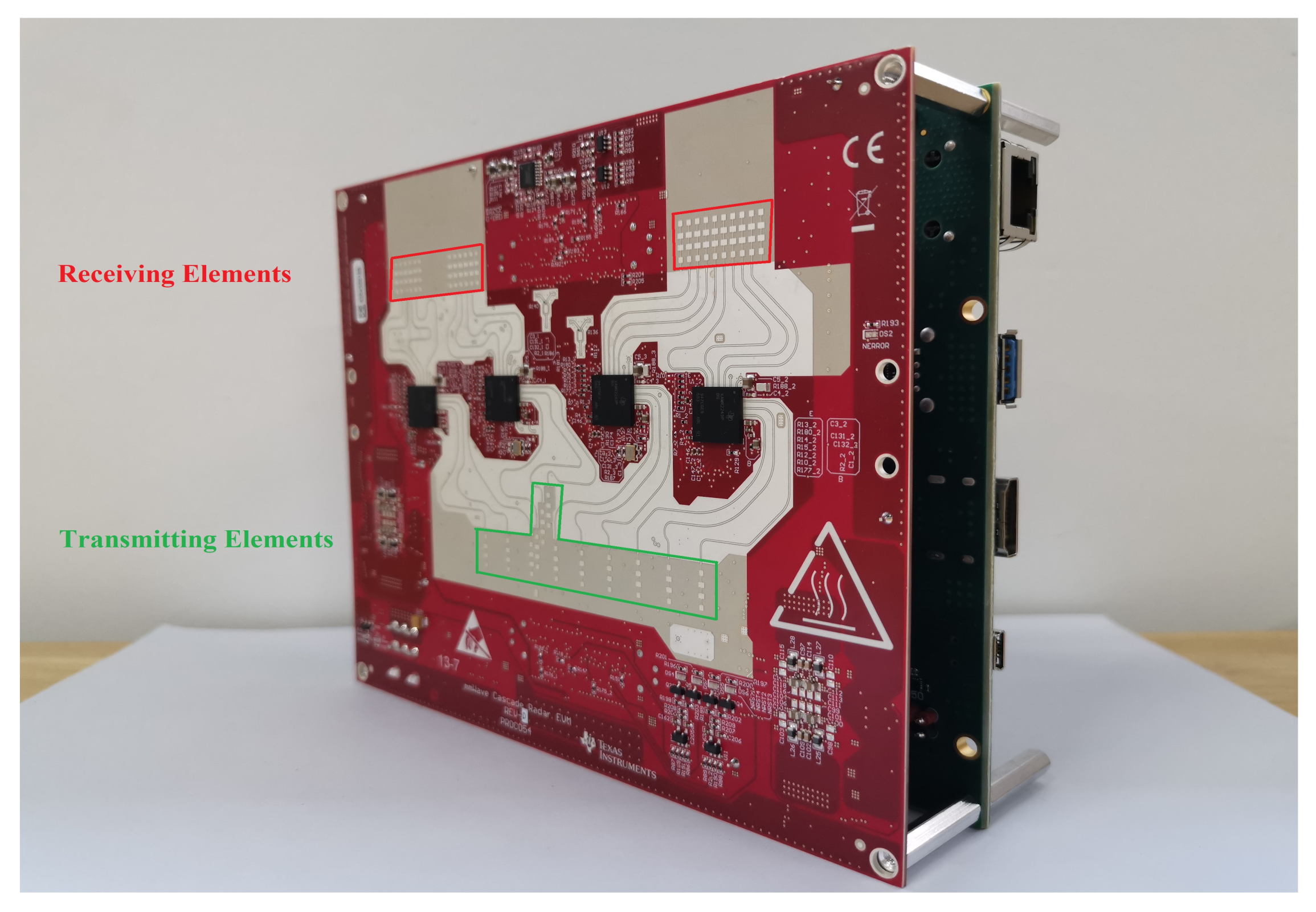
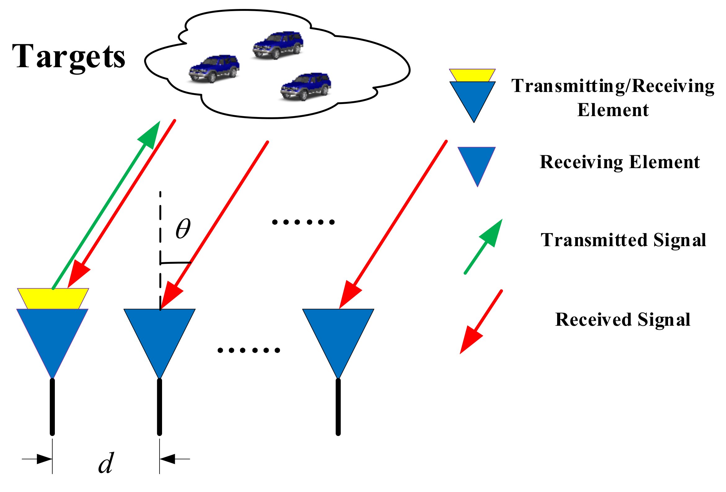
Consider a Texas Instruments (TI) Cascade FMCW MIMO Radar system consisting of MMWAVCAS-RF-EVM and MMWAVCAS-DSP-EVM, shown in Figure 1, with 12 transmitting elements and 16 receiving elements. As shown in Figure 2, the transmitting and receiving elements form a huge virtual array; i.e., each virtual element will be generated at the midpoint of any two transmit and receive elements. denotes wavelength. We selected a row of M purple virtual array elements to form a uniform linear array (ULA).
As shown in Figure 3, where and d denote the DOA and interspacings of the element, respectively, the FMCW signal transmitted from the transmitting element can be expressed as follows:
where and denote the carrier frequency and the slope of the chirps, respectively. For K far-field narrow-band stationary targets, the transmit signal is reflected in K far-field narrow-band stationary targets and the received signal of the m-th receiving element can be represented as:
where is the complex reflection coefficient of the k-th target, is the additive white Gaussian noise (AWGN) at the m-th receiving element and the time delay is the time taken for the signal radiated from the transmitting element to be reflected on the k-th target and received by the m-th receiving element, given as:
where c is the speed of light; is the distance between the transmitting element and k-th target; is the distance between the receiving element and the k-th target; and denotes the DOA of the k-th target. is the relative positions of the m-th receiving element with respect to the transmitting element. Then the time delay can be expressed as:
The received signals are then multiplied by the transmitted signal and run through a low-pass filter (LPF), and with a sampling time ; the can be sampled as:
where is the sampled noise. As , ignoring noise for the moment, the received signal of the m-th element at time n can be expressed as:
Based on Equation (6), for L snapshots, the matrix form of the received signal with additive white Gaussian noise (AWGN) can be expressed as:
where , K, , and is complex Gaussian noise with covariance .
In order to achieve super-resolution imaging, a new receiving data model is obtained by transposition and vectorization:
where , , , , , , .
3. Fast Joint DOA and Range Estimation
Consider the data model of Equation (9). The sampling covariance can be expressed as:
where is the signal covariance.
The above equation can be decomposed into the signal subspace and the noise subspace using eigenvalue decomposition:
where is a diagonal matrix composed of the K largest eigenvalues. is a diagonal matrix composed of the smaller eigenvalues. is the signal subspace composed of the eigenvectors corresponding to the largest K eigenvalues, and is the noise subspace composed of the remaining eigenvectors.
Since the signal subspace is orthogonal to the noise subspace, i.e., , the spatial spectrum function of the 2D-MUSIC algorithm is:
Therefore, the K largest peaks of are the DOA and range estimation of the targets. The computation of 2D-MUSIC focuses on 2D spatial searching and matrix decomposition, whose computational complexities are and , respectively, where q is the number of grids. It can be seen that as the snapshot number and grid density increase, the amount of calculations will grow exponentially, which seriously affects the real-time performance of the system.
To solve this problem, we propose a framework of fast joint DOA and range estimation via Nytrom and VDSR. The structure of the proposed framework is shown in Figure 4, and is divided into four parts: reshaping the received data, using the Nystrom method for estimating subspace, using 2D-MUSIC for low-resolution imaging and using VDSR for reconstructing a high-resolution image.
The reshaping part transforms the original data into the partitioned sampling convariance matrix, as shown in Equations (8) and (10). The signal subspace is obtained using a low-dimensional approximation in the Nystrom part, which reduces the computational load of eigenvalue decomposition. In the 2D-MUSIC part, low-resolution imaging with low grid density is obtained using the signal subspace. The joint DOA and range estimation can be obtained from the VSDR part through a 2D peak search on the high-resolution image.
3.1. Nystrom-Based Low-Resolution Imaging
In this part, the Nystrom method is used to estimate the signal subspace. Then, the 2D-MUSIC spatial spectrum function is formulated based on the signal subspace and the low-resolution image is obtained.
The covariance matrix is partitioned as follows:
where , , , . The approximate signal subspace of the covariance matrix is obtained by using the Nystrom method, which only requires the information of and . Thus, it is not necessary to calculate the covariance matrix . This information can be obtained by partitioning the received data as follows:
where , .
According to Equations (13) and (14), we have:
where and are matrices composed of the first z rows and the last rows of , respectively.
By applying eigenvalue decomposition on , we obtain:
The approximate characteristic matrix is obtained using the Nystrom extension:
In Equation (18), matrix does not satisfy the mutual orthogonality of the column vectors, so the following orthogonalization operation is adopted. Let and decompose the eigenvalue of :
The approximate eigenmatrix satisfying the orthogonality of columns can be obtained as follows:
The approximate signal subspace comprises the last K columns of .
Lemma 1
([22]). We extend the lemma from the array to FMCW MIMO. In the equivalent virtual array of FMCW MIMO radar, if there are K targets, we have , where represents the first K columns of .
Then, can be expressed as:
By introducing Equation (25) into , we have:
As , there exists a nonsingular matrix such that holds. Substituting this matrix into Equation (26), we have:
From the above analysis, we see that in the Nystrom approximate eigenmatrix , where , the first K columns of are independent and and are nonsingular matrices because has a Vandermonde structure. Then, we have:
where represents the first K columns of , and holds.
Using the approximate signal subspace and setting low-density grids, the following 2D-MUSIC spatial spectrum function is formulated:
A low-resolution gray image can be obtained by normalizing the above equation as follows:
where is a matrix in which all elements of the same dimension as are 1.
3.2. VDSR-Based High-Resolution Imaging
VDSR is a CNN architecture designed to perform single-image SR [17]. A VDSR network can elicit the mapping relationship between a high-resolution image and a low-resolution image through a very deep CNN structure. Different from traditional CNNs [21], VDSR aims to reconstruct the residual between the low-resolution image and high-resolution image. This residual contains deep high-frequency information. By using bicubic interpolation to upscale the low-resolution image, the dimensions of the input image and the desired output image can be matched. In addition, we use the bicubic interpolation method to generate the training set. If the interpolation method changes, it only needs to keep the same interpolation algorithm when generating the training set and the actual super-resolution.
The small-size, low-resolution FMCW MIMO radar image obtained using the method of the previous section is gray and can be regarded as an RBG image with only a brightness channel. The VDSR network extracts the residual image from the luminance of a color image; thus, the VDSR framework is very suitable for SR tasks.
As shown in Figure 5, the VDSR is a cascaded pair of convolutional and ReLU layers. It takes an interpolated low-resolution image as input and predicts a residual image as the regression output. By superimposing the images, a high-resolution image can be obtained. It should be noted that to maintain the sizes of all feature maps, zeros need to be padded before convolutions. Some sample feature maps were drawn for visualization, most of which were zero after applying the ReLU.
The detailed structural parameters of the VDSR are shown in Table 2, and the training dataset can be found in [23], and consists of 20,000 natural images. The experimental platform was a PC with an Intel i9-10920X CPU, RTX3090 GPU and 64 GB of RAM. The stochastic gradient descent algorithm with momentum (SGDM) 0.9 and a learning rate of 0.1 was used to reduce learn the rate every 10 epochs. The maximum number of epochs for training was set to 100, and a mini-batch with 64 observations was used at each iteration. Training took about 2.1 h. The training procedure was offline and the training time was not considered in the proposed method.
4. Simulations and Experiments
Several simulations and experiments were carried out to validate the performance of the proposed method. First, we compare the accuracy of the proposed algorithm with the original 2D-MUSIC algorithm [15], and then the computational complexity is verified. Finally, the algorithms were applied to experimental data. The TI Cascade FMCW MIMO Radar parameters shared by the simulations and experiments are shown in Table 3.
4.1. Simulations
To verify the performance of the overall framework, consider two far-field narrow-band stationary targets at and . The locationing effect was evaluated using the root mean square error (RMSE) metric. Differently from the single parameter estimation in [24,25], for the multi-parameter estimation problem, we defined the RMSE of the DOA and the RMSE of the range as follows:
where and are the k- actual DOA and range, and , and are the k- estimated values of DOA and range in the t- Monte Carlo (MC) trial. The selection of the number of MC depends on the stability of the algorithm. When the number of MC experiments is large enough, the RMSE curves of the estimated parameters remain almost unchanged. After the number of MC experiments exceeds 200, the RMSE curve of the proposed algorithm and the comparison algorithm no longer changes with the increase of the number of MC experiments, so the number of MC experiments was set to 200. In addition, the running time of the algorithm was selected as performance metric of the real-time performance of the algorithms.
For the sake of fairness, we considered the original 2D-MUSIC with different grids of , and , . We set the low-density grid for the proposed algorithm in the first stage as , and the super-resolution high-density as , . The parameter z of the Nystrom method for solving the approximate signal subspace was 86, and the number of snapshots was 75. As shown in Figure 6 and Figure 7, the RMSE of the proposed algorithm is better than that of 2D-MUSIC with a low-density grid but worse than that of 2D-MUSIC with a high-density grid. Due to the existence of grid errors, the estimation error of 2D-MUSIC with grids of , cannot be reduced beyond a certain value through the increase of SNR. Moreover, as shown in Figure 8, the runtime of our proposed algorithm was shorter than that of 2D-MUSIC.
4.2. Experiments
The experimental data were from the TI Cascade FMCW MIMO Radar shown in Figure 1. The experimental site was a microwave anechoic chamber with metal reflectors. The number of snapshots was 75. First, the 2D-MUSIC algorithm is compared with the Nystrom-based 2D-MUSIC algorithm, and then the 2D-MUSIC algorithm is compared with the VDSR-based 2D-MUSIC algorithm.
4.2.1. Comparisons of the 2D-MUSIC Algorithm and the Nystrom-Based 2D-MUSIC Algorithm
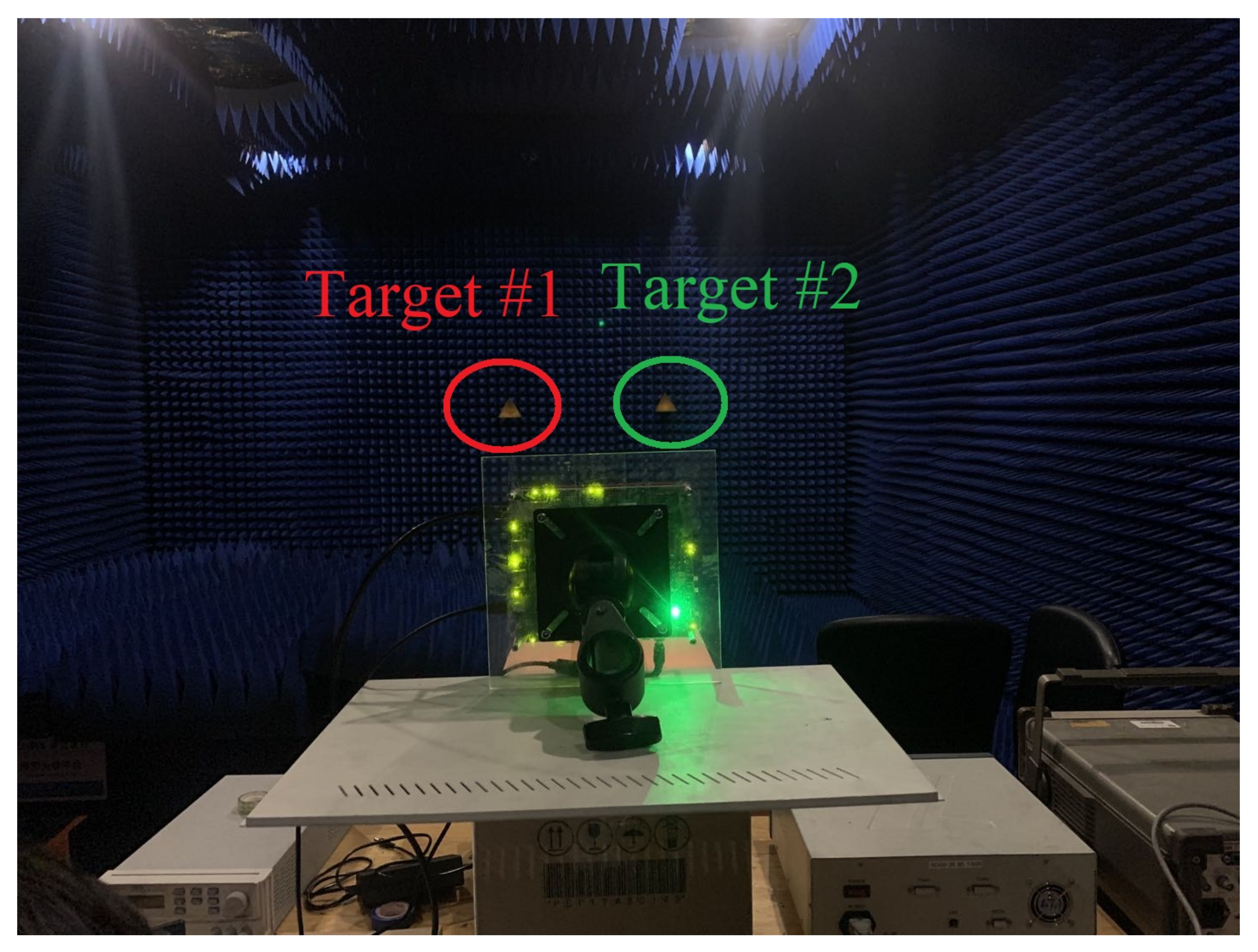
As shown in Figure 9 and Figure 10, we set up two scenarios, one with a single target at and one with two targets at , respectively. In this part, the locationing effect was selected as the performance metric.
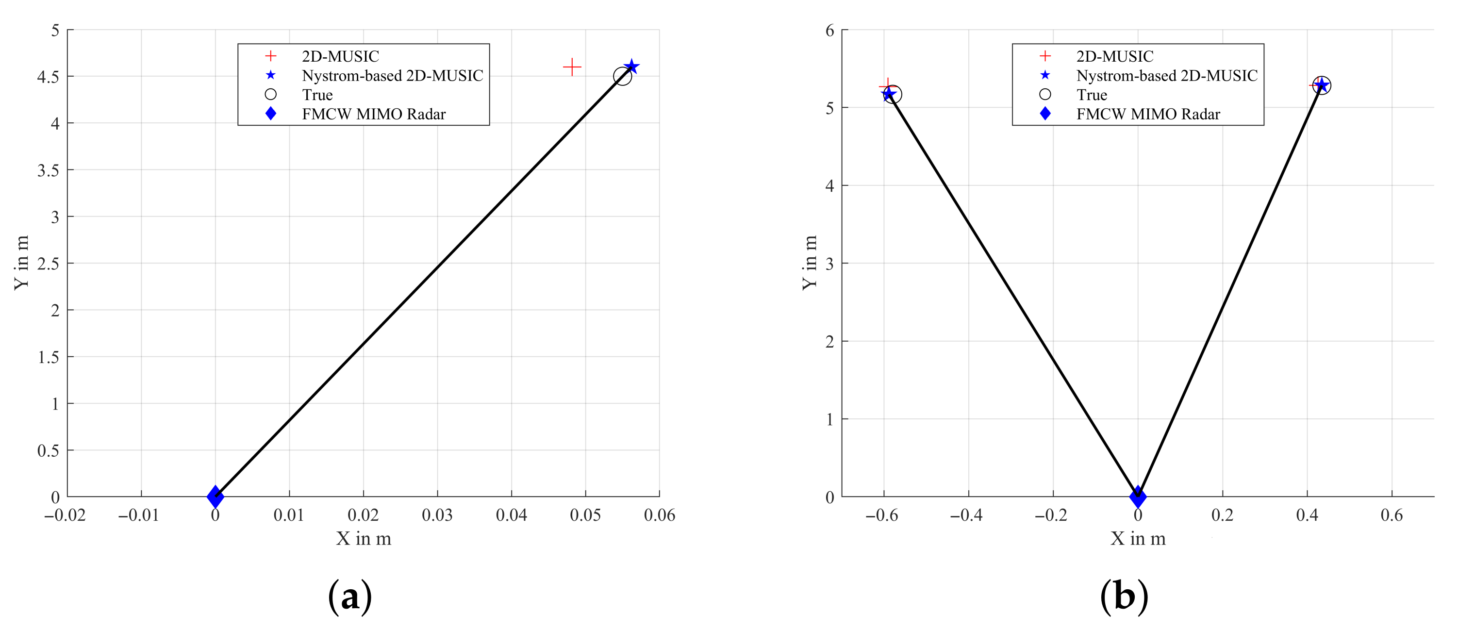
We set the grid for both the original 2D-MUSIC algorithm and the Nystrom-based 2D-MUSIC algorithm as , . As shown in Figure 11a–d, although the Nystrom-based 2D-MUSIC algorithm has more sidelobes than that of the 2D-MUSIC algorithm, it does not affect target discrimination.
Figure 12a,b shows comparisons between 2D-MUSIC algorithm and the Nystrom-based 2D-MUSIC algorithm for the localization results of one and two targets with experimental data. It can be seen from the figures that the performance of the Nystrom-based 2D-MUSIC algorithm is similar to that of 2D-MUSIC, which shows that the subspace obtained by Nystrom method has high accuracy in practical applications.
4.2.2. Comparisons of the 2D-MUSIC Algorithm and the VDSR-Based 2D-MUSIC Algorithm
As shown in Figure 13 and Figure 14, we set up two scenarios, one with a single target at and one with two targets at , respectively. In this part, the locationing effect and running time were selected as performance metrics.
To obtain the low-resolution image, the low-density intervals were set as , . Figure 15a,b shows the low-resolution imaging results obtained from the experimental data of one and two targets, respectively, using the method proposed in Section 3.1. It is obvious that the peak value in the 2D image does not represent the targets’ positions accurately due to the large grid division.
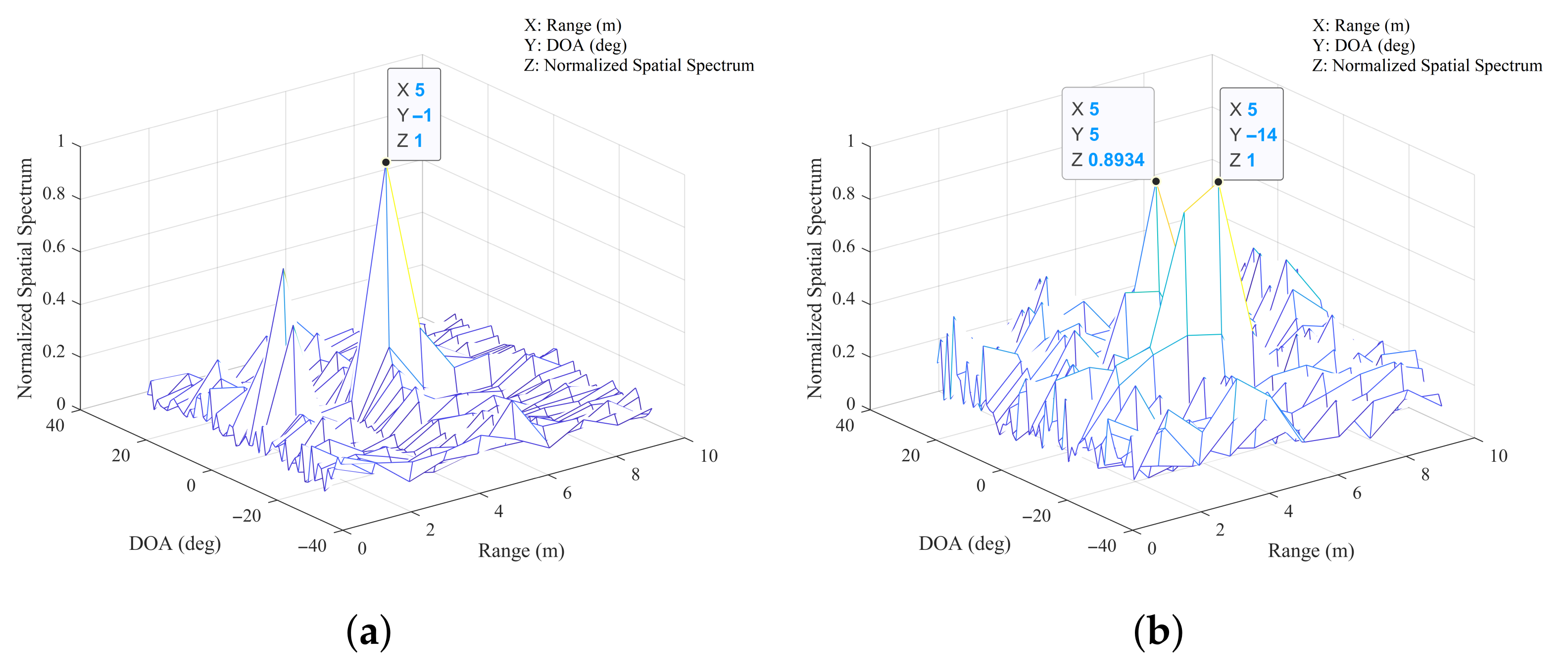
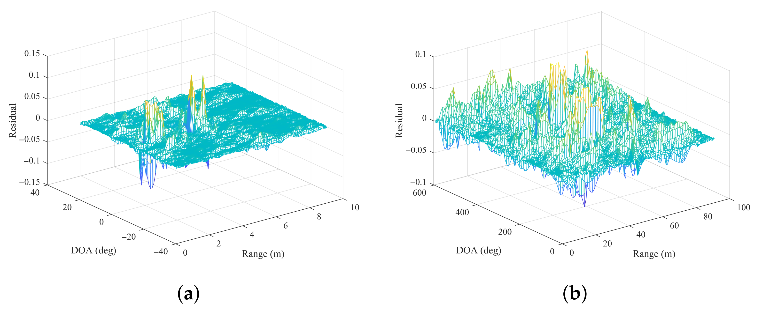
Figure 16a,b shows the residual images obtained via VDSR from the low-resolution images of the one and two-target experimental data, with resolutions of and , respectively. It can be obviously observed that the missing high-frequency information of the low-resolution image was reconstructed to correct the peaks and edges.
Figure 17a,b shows the high-resolution images of the single and double-target experimental data, respectively, which complement the details of the low-resolution images. As can be seen from the figures, the image peaks are not very sharp, which indicates that with the decrease of the distance between targets, the grid needs to be further refined to achieve better results also.
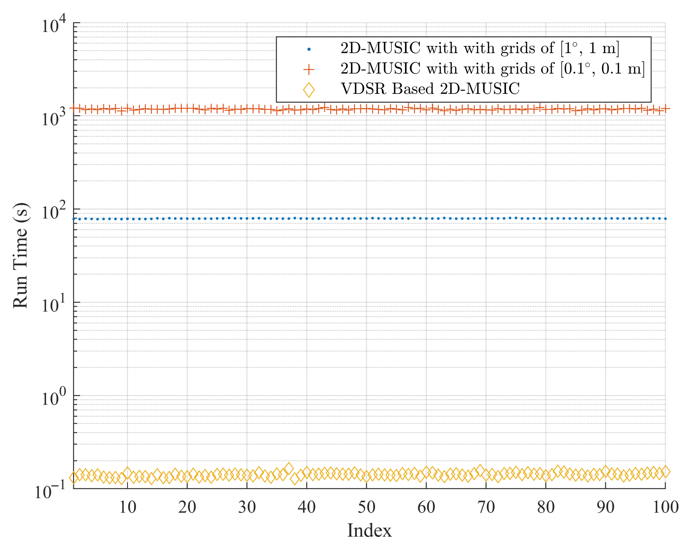
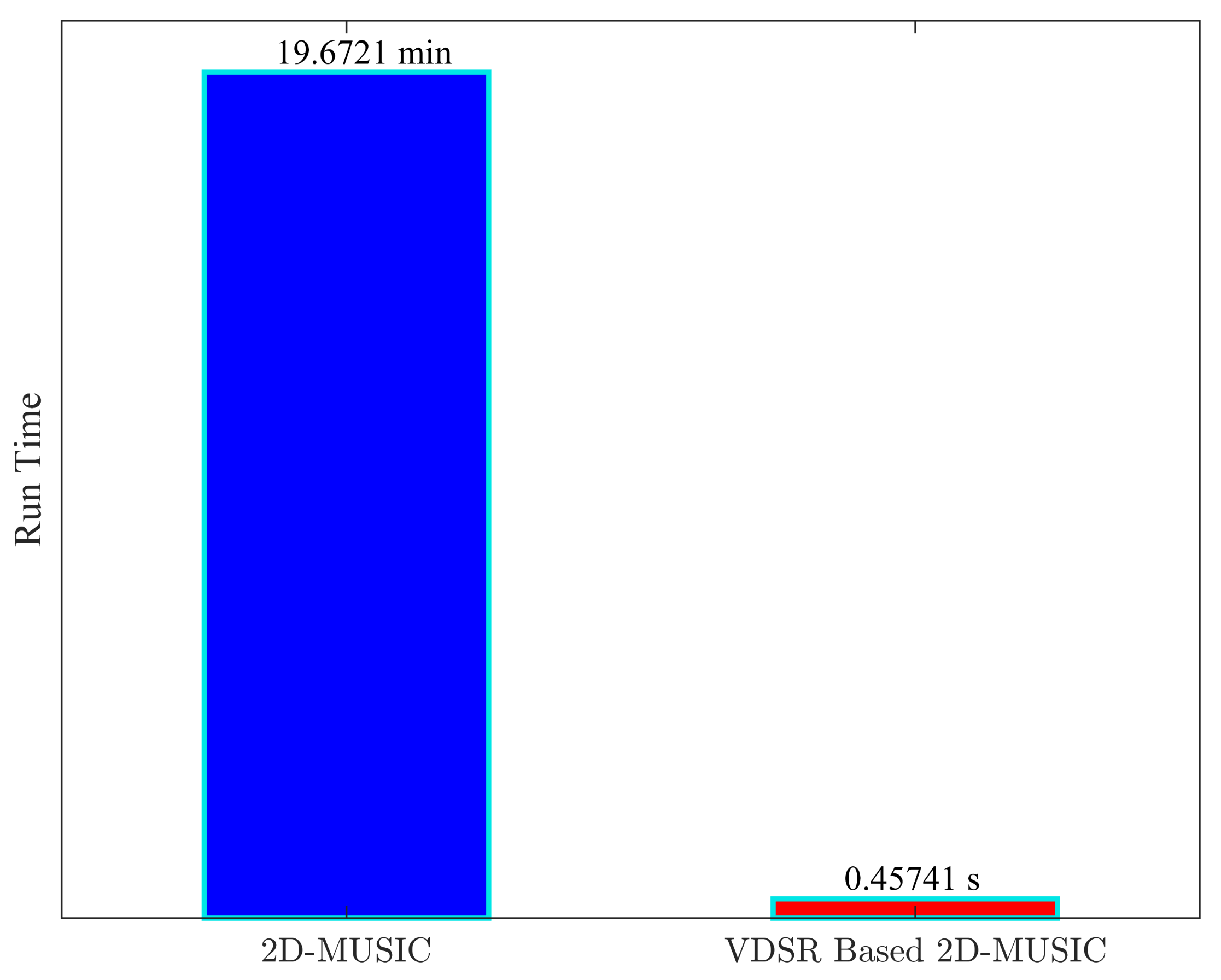
As the validation of experimental data does not require a large number of Monte Carlo experiments, a fine grid , was adopted. As shown in Figure 18, the estimation with 2D-MUSIC needed several minutes; in contrast, the proposed algorithm only took , which shows the real-time advantage of the algorithm. Figure 19a,b shows the imaging results of the one and two-target experimental data obtained using the original 2D-MUSIC. It can be seen that with a complete noise subspace and a fine grid, 2D-MUSIC can achieve very sharp spatial spectrum peaks. However, these results are obtained at the cost of extremely long running times, and the real-time performance is extremely poor.
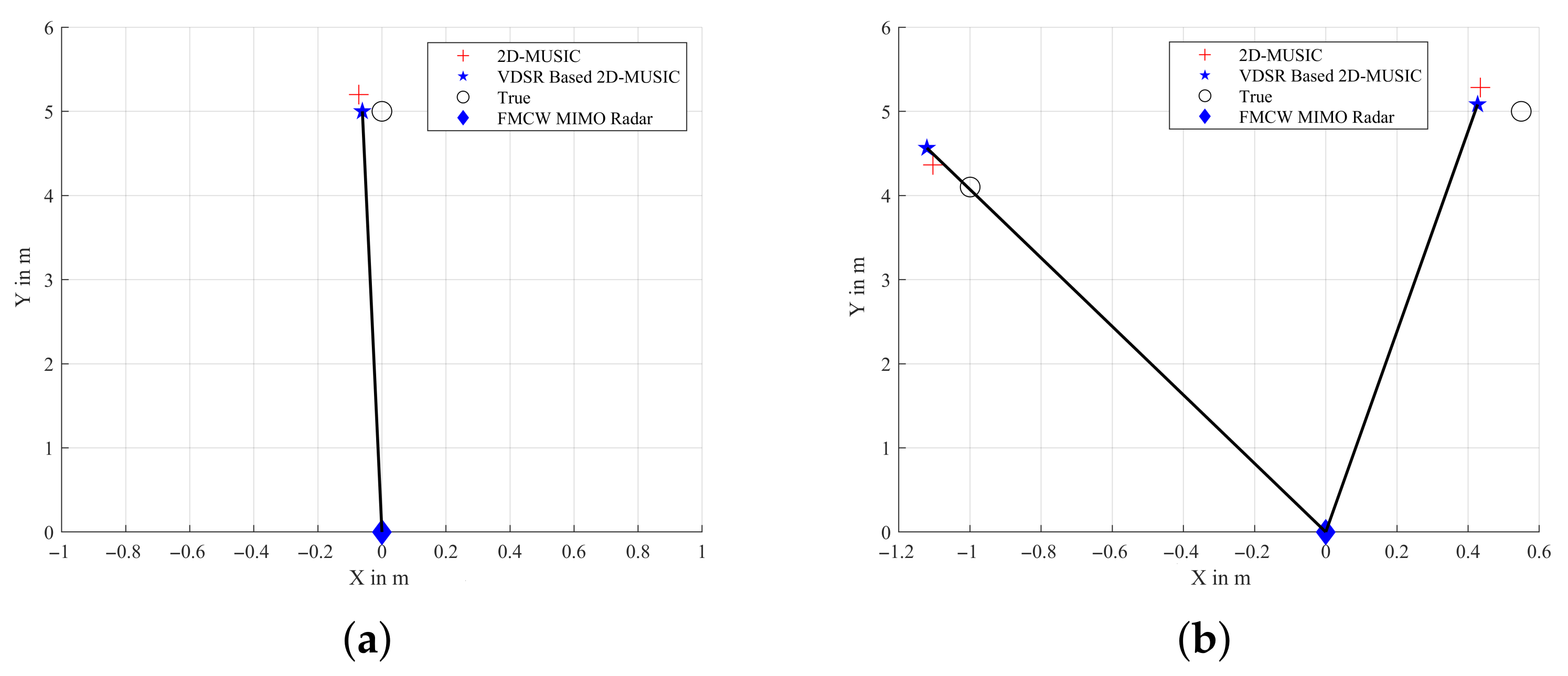
Figure 20a,b shows comparisons between the 2D-MUSIC algorithm and the proposed algorithm for the localization results of one and two targets with experimental data. It can be seen from the figures that the performance of the proposed algorithm is similar to that of 2D-MUSIC, despite the fact that our algorithm is much faster than 2D-MUSIC. In addition, as both algorithms present similar offsets, the calibration of the radar needs to be improved in future work.
5. Conclusions
In this paper, a fast joint direction-of-arrival (DOA) and range estimation framework for target localization based on a VDSR neural network was proposed. With the proposed algorithm, both the estimation error and the running time can be effectively decreased. Simulations and experiments have proved that real-time performance of the proposed algorithm is more plausible than with the traditional 2D-MUSIC algorithm. Although the proposed method has achieved good results, it is still limited to the X86 platform and has not been implemented in embedded hardware such as FPGA. In addition, the network structure is not optimal. Some excellent compact network structures in [26,27] could be used to further improve network efficiency. Therefore, in future work, improvements to this method will be made, and real-time signal processing will be implemented on the embedded hardware platform.
Author Contributions
Writing—original draft preparation, methodology, software, J.C.; conceptualization, supervision, methodology, X.W.; investigation, project administration, X.L. and L.W.; funding acquisition, M.H. and X.W. All authors have read and agreed to the published version of the manuscript.
Funding
This work was supported by the National Natural Science Foundation of China (number 61861015 and 61961013), the Key Research and Development Program of Hainan Province (number ZDYF2019011), the National Key Research and Development Program of China (number 2019CXTD400), the Young Elite Scientists Sponsorship Program by CAST (number 2018QNRC001) and the Scientific Research Setup Fund of Hainan University (number KYQD(ZR) 1731).
Institutional Review Board Statement
Not applicable.
Informed Consent Statement
Not applicable.
Data Availability Statement
Not applicable.
Acknowledgments
Not applicable.
Conflicts of Interest
The authors declare no conflict of interest.
References
- Skolnik, M. Introduction to radar. In Radar Handbook; McGraw-Hill Book Co: New York, NY, USA, 1962; p. 22. [Google Scholar]
- Hasch, J.; Topak, E.; Schnabel, R.; Zwick, T.; Weigel, R.; Waldschmidt, C. Millimeter-Wave Technology for Automotive Radar Sensors in the 77 GHz Frequency Band. IEEE Trans. Microw. Theory Tech. 2012, 60, 845–860. [Google Scholar] [CrossRef]
- Rohling, H.; Meinecke, M. Waveform design principles for automotive radar systems. In Proceedings of the 2001 CIE International Conference on Radar Proceedings (Cat No.01TH8559), Beijing, China, 15–18 October 2001; pp. 1–4. [Google Scholar]
- Schneider, M. Automotive radar-status and trends. In Proceedings of the German Microwave Conference, Munich, Germany, 5–7 April 2005; pp. 144–147. [Google Scholar]
- Esposito, C.; Berardino, P.; Natale, A.; Perna, S. On the Frequency Sweep Rate Estimation in Airborne FMCW SAR Systems. Remote Sens. 2020, 12, 3448. [Google Scholar] [CrossRef]
- Esposito, C.; Natale, A.; Palmese, G.; Berardino, P.; Lanari, R.; Perna, S. On the Capabilities of the Italian Airborne FMCW AXIS InSAR System. Remote Sens. 2020, 12, 539. [Google Scholar] [CrossRef] [Green Version]
- Wang, R.; Loffeld, O.; Nies, H.; Knedlik, S.; Hagelen, M.; Essen, H. Focus FMCW SAR Data Using the Wavenumber Domain Algorithm. IEEE Trans. Geosci. Remote Sens. 2010, 48, 2109–2118. [Google Scholar] [CrossRef]
- Giusti, E.; Martorella, M. Range Doppler and Image Autofocusing for FMCW Inverse Synthetic Aperture Radar. IEEE Trans. Aerosp. Electron. Syst. 2011, 47, 2807–2823. [Google Scholar] [CrossRef]
- Liu, Y.; Deng, Y.K.; Wang, R.; Loffeld, O. Bistatic FMCW SAR Signal Model and Imaging Approach. IEEE Trans. Aerosp. Electron. Syst. 2013, 49, 2017–2028. [Google Scholar] [CrossRef]
- Stove, A. Linear FMCW radar techniques. IEE Proc. F (Radar Signal Process.) 1992, 139, 343–350. [Google Scholar] [CrossRef]
- Brennan, P.; Huang, Y.; Ash, M.; Chetty, K. Determination of Sweep Linearity Requirements in FMCW Radar Systems Based on Simple Voltage-Controlled Oscillator Sources. IEEE Trans. Aerosp. Electron. Syst. 2011, 47, 1594–1604. [Google Scholar] [CrossRef]
- Wang, X.; Wan, L.; Huang, M.; Shen, C.; Han, Z.; Zhu, T. Low-complexity channel estimation for circular and noncircular signals in virtual MIMO vehicle communication systems. IEEE Trans. Veh. Technol. 2021, 69, 3916–3928. [Google Scholar] [CrossRef]
- Feger, R.; Wagner, C.; Schuster, S.; Scheiblhofer, S.; Jager, H.; Stelzer, A. A 77-GHz FMCW MIMO Radar Based on an SiGe Single-Chip Transceiver. IEEE Trans. Microw. Theory Tech. 2009, 57, 1020–1035. [Google Scholar] [CrossRef]
- Wang, X.; Huang, M.; Wan, L. Joint 2D-DOD and 2D-DOA Estimation for Coprime EMVS–MIMO Radar. Circuits Syst. Signal Process. 2021. [Google Scholar] [CrossRef]
- Belfiori, F.; van Rossum, W.; Hoogeboom, P. 2D-MUSIC technique applied to a coherent FMCW MIMO radar. In Proceedings of the IET International Conference on Radar Systems (Radar 2012), Glasgow, UK, 22–25 October 2012; pp. 1–6. [Google Scholar]
- Hamidi, S.; Nezhad-Ahmadi, M.; Safavi-Naeini, S. TDM based Virtual FMCW MIMO Radar Imaging at 79GHz. In Proceedings of the 2018 18th International Symposium on Antenna Technology and Applied Electromagnetics (ANTEM), Waterloo, ON, Canada, 19–22 August 2018; pp. 1–2. [Google Scholar]
- Kim, J.; Lee, J.K.; Lee, K.M. Accurate Image Super-Resolution Using Very Deep Convolutional Networks. In Proceedings of the 2016 IEEE Conference on Computer Vision and Pattern Recognition (CVPR), Las Vegas, NV, USA, 27–30 June 2016; pp. 1646–1654. [Google Scholar]
- Timofte, R.; Smet, V.; Gool, H. A+: Adjusted anchored neighborhood regression for fast super-resolution. In Proceedings of the Asian Conference on Computer Vision, Singapore, 1–5 November 2014; Springer: Cham, Switzerland, 2014; pp. 111–126. [Google Scholar]
- Schulter, S.; Leistner, C.; Bischof, H. Fast and accurate image upscaling with super-resolution forests. In Proceedings of the 2015 IEEE Conference on Computer Vision and Pattern Recognition (CVPR), Boston, MA, USA, 7–12 June 2015; pp. 3791–3799. [Google Scholar]
- Huang, J.; Singh, A.; Ahuja, N. Single image super-resolution from transformed self-exemplars. In Proceedings of the 2015 IEEE Conference on Computer Vision and Pattern Recognition (CVPR), Boston, MA, USA, 7–12 June 2015; pp. 5197–5206. [Google Scholar]
- Dong, C.; Loy, C.; He, K.; Tang, X. Image Super-Resolution Using Deep Convolutional Networks. IEEE Trans. Pattern Anal. Mach. Intell. 2016, 38, 295–307. [Google Scholar] [CrossRef] [PubMed] [Green Version]
- Wang, X.; Huang, M.; Cao, C.; Li, H. Angle Estimation of Noncircular Source in MIMO Radar via Unitary Nystrom Method. In Proceedings of the International Conference in Communications, Signal Processing, and Systems, Harbin, China, 14–16 July 2017; Springer: Singapore, 2017. [Google Scholar]
- Grubinger, M.; Clough, P.; Müller, H.; Deselaers, T. The IAPR TC12 Benchmark: A New Evaluation Resource for Visual Information Systems. In Proceedings of the OntoImage 2006 Language Resources for Content-Based Image Retrieval, Genoa, Italy, 22 May 2006; Volume 5, p. 10. [Google Scholar]
- Cong, J.; Wang, X.; Huang, M.; Wan, L. Robust DOA Estimation Method for MIMO Radar via Deep Neural Networks. IEEE Sensors J. 2021, 21, 7498–7507. [Google Scholar] [CrossRef]
- Wang, X.; Yang, L.T.; Meng, D.; Dong, M.; Ota, K.; Wang, H. Multi-UAV Cooperative Localization for Marine Targets Based on Weighted Subspace Fitting in SAGIN Environment. IEEE Internet Things J. 2021. [Google Scholar] [CrossRef]
- Winoto, A.S.; Kristianus, M.; Premachandra, C. Small and Slim Deep Convolutional Neural Network for Mobile Device. IEEE Access 2020, 8, 125210–125222. [Google Scholar] [CrossRef]
- Baozhou, Z.; Al-Ars, Z.; Hofstee, H.P. REAF: Reducing Approximation of Channels by Reducing Feature Reuse within Convolution. IEEE Access 2020, 8, 169957–169965. [Google Scholar] [CrossRef]
Figure 1.
TI Cascade FMCW MIMO Radar system.

Figure 2.
Virtual antenna array of TI Cascade FMCW MIMO Radar.

Figure 3.
A schematic diagram of the target localization system.

Figure 4.
The structure of the proposed framework.

Figure 5.
The structure of VDSR.

Figure 6.
RMSE of DOA versus SNR.

Figure 7.
RMSE of DOA versus SNR.

Figure 8.
Simulation runtime.

Figure 9.
Single target scenario.

Figure 10.
Double target scenario.

Figure 11.
Imaging: (a) Single target with Nystrom-based 2D-MUSIC. (b) Two targets with Nystrom-based 2D-MUSIC. (c) Single target with 2D-MUSIC. (d) Two targets with 2D-MUSIC.
Figure 11.
Imaging: (a) Single target with Nystrom-based 2D-MUSIC. (b) Two targets with Nystrom-based 2D-MUSIC. (c) Single target with 2D-MUSIC. (d) Two targets with 2D-MUSIC.

Figure 12.
A comparison of target localization Results: (a) Single target. (b) Two Targets.

Figure 13.
Single-target scenario for dataset collection.

Figure 14.
Two-target scenario for dataset collection.

Figure 15.
Low-resolution imaging: (a) Single target. (b) Two targets.

Figure 16.
Residuals of low-resolution: (a) Single target. (b) Two targets.

Figure 17.
High-resolution imaging results: (a) Single target. (b) Two targets.

Figure 18.
Experimental runtime.

Figure 19.
2D-MUSIC imaging results with a fine grid: (a) Single target. (b) Two targets.

Figure 20.
A comparison of target localization results: (a) Single target. (b) Two targets.


Table 1.
Related notation.
| Notations | Definitions |
|---|---|
| capital bold italic letters | matrices |
| lowercase bold italic letters | vectors |
| j | imaginary unit |
| e | Euler number |
| t | time |
| conjugate transpose operator | |
| transpose operator | |
| vectorization operator | |
| dimensional complex matrix set | |
| 2-norm operator | |
| mathematical expectation | |
| ⊗ | Kronecker product |
| ⊙ | Khatri-Rao product |
| Moore-Penrose Inverse | |
| expansion space operator | |
| minimum value | |
| maximum value | |
| Identity matrix of order M | |
| Rectified Linear Units |
Table 2.
Detailed structural parameters of VDSR.
| Name | Type | Activations | Learnables |
|---|---|---|---|
| Input Image | Image Input | - | |
| Image Size: | |||
| Conv.1 | Convolution | Weights | |
| Number of Filters: 64, Filter Size: | |||
| with stride [1 1] and padding [1 1 1 1] | Bias | ||
| ReLU.1 | ReLU | - | |
| Conv.2 | Convolution | Weights | |
| Number of Filters: 64, Filter Size: | |||
| with stride [1 1] and padding [1 1 1 1] | Bias | ||
| ReLU.2 | ReLU | - | |
| Conv.3 | Convolution | Weights | |
| Number of Filters: 64, Filter Size: | |||
| with stride [1 1] and padding [1 1 1 1] | Bias | ||
| ReLU.3 | ReLU | - | |
| … | … | … | … |
| Conv.19 | Convolution | Weights | |
| Number of Filters: 64, Filter Size: | |||
| with stride [1 1] and padding [1 1 1 1] | Bias | ||
| ReLU.19 | ReLU | - | |
| Conv.20 | Convolution | Weights | |
| Number of Filters: 1, Filter Size: | |||
| with stride [1 1] and padding [1 1 1 1] | Bias | ||
| Residual Output | Regression Output | - | - |
| mean-squared-error | |||
| with response “ResponseImage” |
Table 3.
TI Cascade FMCW MIMO Radar parameters.
| Parameter | Value | Parameter | Value |
|---|---|---|---|
| c | |||
| d | M | 86 | |
| L | 75 |
Publisher’s Note: MDPI stays neutral with regard to jurisdictional claims in published maps and institutional affiliations. |
© 2021 by the authors. Licensee MDPI, Basel, Switzerland. This article is an open access article distributed under the terms and conditions of the Creative Commons Attribution (CC BY) license (https://creativecommons.org/licenses/by/4.0/).
Share and Cite
MDPI and ACS Style
Cong, J.; Wang, X.; Lan, X.; Huang, M.; Wan, L. Fast Target Localization Method for FMCW MIMO Radar via VDSR Neural Network. Remote Sens. 2021, 13, 1956. https://0-doi-org.brum.beds.ac.uk/10.3390/rs13101956
AMA Style
Cong J, Wang X, Lan X, Huang M, Wan L. Fast Target Localization Method for FMCW MIMO Radar via VDSR Neural Network. Remote Sensing. 2021; 13(10):1956. https://0-doi-org.brum.beds.ac.uk/10.3390/rs13101956
Chicago/Turabian StyleCong, Jingyu, Xianpeng Wang, Xiang Lan, Mengxing Huang, and Liangtian Wan. 2021. "Fast Target Localization Method for FMCW MIMO Radar via VDSR Neural Network" Remote Sensing 13, no. 10: 1956. https://0-doi-org.brum.beds.ac.uk/10.3390/rs13101956
Note that from the first issue of 2016, this journal uses article numbers instead of page numbers. See further details here.