
Application of Machine-Learning-Based Fusion Model in Visibility Forecast: A Case Study of Shanghai, China

1
Shanghai Typhoon Institute, Shanghai Meteorological Service, Shanghai 200030, China
2
Shanghai Key Laboratory of Meteorology and Health, Shanghai Meteorological Service, Shanghai 200030, China
3
Department of Atmospheric and Oceanic Sciences, Institute of Atmospheric Sciences, Fudan University, Shanghai 200438, China
*
Author to whom correspondence should be addressed.
Remote Sens. 2021, 13(11), 2096; https://0-doi-org.brum.beds.ac.uk/10.3390/rs13112096
Submission received: 4 April 2021
/
Revised: 14 May 2021
/
Accepted: 22 May 2021
/
Published: 27 May 2021
(This article belongs to the Special Issue Artificial Intelligence in Remote Sensing of Atmospheric Environment)
Abstract
:A visibility forecast model called a boosting-based fusion model (BFM) was established in this study. The model uses a fusion machine learning model based on multisource data, including air pollutants, meteorological observations, moderate resolution imaging spectroradiometer (MODIS) aerosol optical depth (AOD) data, and an operational regional atmospheric environmental modeling System for eastern China (RAEMS) outputs. Extreme gradient boosting (XGBoost), a light gradient boosting machine (LightGBM), and a numerical prediction method, i.e., RAEMS were fused to establish this prediction model. Three sets of prediction models, that is, BFM, LightGBM based on multisource data (LGBM), and RAEMS, were used to conduct visibility prediction tasks. The training set was from 1 January 2015 to 31 December 2018 and used several data pre-processing methods, including a synthetic minority over-sampling technique (SMOTE) data resampling, a loss function adjustment, and a 10-fold cross verification. Moreover, apart from the basic features (variables), more spatial and temporal gradient features were considered. The testing set was from 1 January to 31 December 2019 and was adopted to validate the feasibility of the BFM, LGBM, and RAEMS. Statistical indicators confirmed that the machine learning methods improved the RAEMS forecast significantly and consistently. The root mean square error and correlation coefficient of BFM for the next 24/48 h were 5.01/5.47 km and 0.80/0.77, respectively, which were much higher than those of RAEMS. The statistics and binary score analysis for different areas in Shanghai also proved the reliability and accuracy of using BFM, particularly in low-visibility forecasting. Overall, BFM is a suitable tool for predicting the visibility. It provides a more accurate visibility forecast for the next 24 and 48 h in Shanghai than LGBM and RAEMS. The results of this study provide support for real-time operational visibility forecasts.
1. Introduction
Visibility indicates the transparency of the atmosphere and is closely related to the daily life of the public. Low visibility, including precipitation, fog, haze, dust, and smoke, is a meteorological disaster that affects all forms of transport, particularly within the fields of land, aviation, and shipping, and causes casualties and property losses [1,2,3,4]. As a result, the study of atmospheric visibility has been a significant public concern. Visibility forecasts are complicated and dominated by meteorological conditions, such as particulate matter, relative humidity, wind speed, and wind direction [5,6]. At present, several approaches are commonly used to predict atmospheric visibility, including meteorological numerical forecasting and statistical forecasting based on machine learning. Numerical forecasts based on meteorology and atmospheric chemistry, such as weather research and forecasting models coupled with chemistry (WRF-Chem) [7,8], the community multiscale air quality (CMAQ) model [9,10], and the CMA Unified Atmosphere Chemistry Environment (CUACE) [11] were developed to conduct real-time operational visibility and atmospheric pollutant forecasts. In fact, to determine the uncertainties of numerical model forecast, detailed regional emissions and suitable physical and chemical schemes are both required based on a deep understanding of physical and chemical mechanisms [12]. It is difficult to accurately quantify every atmospheric process theoretically because of the complexity of the atmosphere, which leads to large errors and uncertainties during prediction [13,14,15].
The second approach to visibility prediction is statistical forecasting based on machine learning methods, which is a branch of artificial intelligence [16,17], studies on the mechanism of human cognition, and the establishment of various learning models with the support of computer systems. Comparing with traditional statistical methods, a non-linear regression prediction based on machine learning forecast method performs better to some extent because machine learning methods do not require a time-consuming model selection for each different cell and reduce large forecasting errors [18,19]. The availability of large datasets also improves the forecasting performance [20]. Machine learning algorithms have been applied to environmental and meteorological forecasting and research in recent years [21,22,23,24,25,26,27]. Such algorithms detect and predict meteorological phenomena, including poor visibility events [28]. Several trials using machine learning to predict the visibility have been conducted by researchers and forecasters, such as artificial networks [29], tree-based methods [30], and multiple linear regression [31]. To date, previous studies on forecasting visibility have often used a single machine learning algorithm and meteorological historical data to determine the relationship between visibility and other observations. However, many other factors that contribute to local visibility forecast have not been considered.
Machine learning model fusion is an effective method of constructing multiple base classifiers (using multiple machine learning algorithms) and then combining them to complete a learning task and solve a particular computational problem [32,33]. Specifically, when the error rates of each base classifier are independent of each other, the error rate of the model fusion decreases exponentially to zero. In fact, each classifier is the result of solving the same problem, and the error rate has difficulty being independent. For the same problem, the more accurate the base classifier, the more similar it will be. As a result, classifiers that are too strong will significantly affect the following results and may even make it impossible to apply the following classifiers. Logistic regression [34] and support vector machines [35] are typical base classifiers. Machine-learning-based model fusion shows a better accuracy than other single machine learning algorithms, but with more complexity and lower efficiency. According to the relationship between learners, machine-learning-based fusion models can be divided into two categories: a serialization method with strong dependence among learners, as represented by boosting [36], and a parallel method with independent learners, as represented by bagging [37]. Boosting algorithms include AdaBoost [38], the gradient boosting decision tree (GBDT) method [39], XGBoost [40], LightGBM [41], CatBoost [42], and random forest [43]. Unlike the bagging algorithm, the boosting algorithm tries to add new classifiers where previous classifiers have failed. Boosting also determines the weights for the data and reduces the model bias [44].
Although model fusion has been used in several fields of meteorology [18,45,46], it has not been widely used to predict the visibility in China. Shanghai is in the east of China and has a huge population. The visibility trends of Shanghai, along with important meteorological and environmental factors, were investigated. Since 2000, the percentage of bad visibility days (visibility <5 km) fluctuated, peeking in 2003 and 2015, and the number of good visibility days (visibility >15 km) has declined significantly since 2012 [6]. It is important to conduct accurate visibility forecasting in Shanghai to support disaster prevention and mitigation of this megacity. The Shanghai Meteorological Service (SMS) currently runs RAEMS based on WRF-Chem operational modeling to forecast daily environmental atmospheric pollutants and visibility [8]. However, large uncertainties still exist in numerical model predictions.
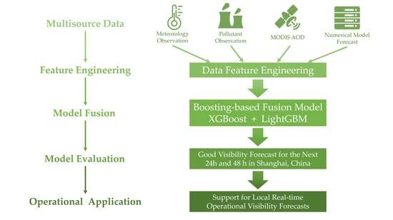
The aim of this study is to build a new fusion model based on multisource data to improve visibility forecast. Single classification and regression methods using historical observed data do not meet the prediction accuracy requirements for local visibility forecasts. In this study, a new model for visibility prediction was established using a machine-learning-based model fusion based on operational regional atmospheric environmental modelling system for eastern China (RAEMS) outputs, air pollutants, meteorological observations, and MODIS AOD data. Machine learning and numerical prediction methods were combined to build a new model. The new model uses two machine learning algorithms (XGBoost and LightGBM), and several special data processes are applied. We named this new model the boosting-based fusion model (BFM). The performance of this BFM prediction was compared with the predictions of the LightGBM model based on RAEMS and RAEMS itself.
2. Materials and Methods
2.1. Data Introduction
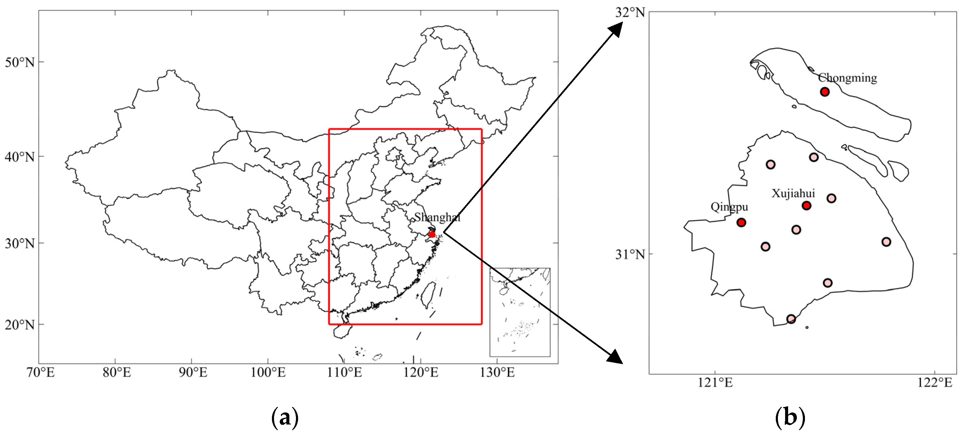
In this study, meteorological observational data and RAEMS modeling forecast data were collected from the Shanghai Meteorological Service. Observational pollutant data were obtained from the Shanghai Municipal Bureau of Ecology and Environment. The data covered 5 years from 1 January 2015 to 31 December 2019, with a time granularity of 1 h. Eleven national synoptic stations provided observed meteorological variables (Figure 1). The meteorological data included surface visibility, temperature, pressure, relative humidity, precipitation, wind speed, wind direction, and radiation-related factors. The national environmental stations provided six basic observational pollutant variables, i.e., PM2.5, PM10, O3, NOx, CO, and SO2. In addition, RAEMS provided both surface and high-level meteorological and chemical forecast variables. The RAEMS surface forecast data included meteorological variables and the six air pollutants mentioned above. The RAEMS high-level forecast meteorological variables were collected at 1000, 925, 850, 700, and 500 hPa. The details of RAEMS were introduced in Section 2.2.
Moreover, because aerosol optical depth characterizes atmospheric turbidity, which is highly related to visibility, MODIS AOD data from National Aeronautics and Space Administration (NASA) were involved in this study [47]. The MODIS AOD data, MCD19A2, was a multi-angle implementation of atmospheric correction (MAIAC) algorithm-based gridded aerosol optical depth product. This product was generated by using the Ross-Thick Li-Sparse (RTLS) bi-directional reflectance distribution function (BRDF), spectral surface albedo, bidirectional reflectance factors (BRF), and the semi-analytical Green’s function solution models [48,49,50,51]. It was derived by Terra and Aqua MODIS inputs. It provided daily AOD data with a spatial resolution of 1 km from 1 January 2015 to 31 December 2019. In this study, we used the AOD data at 0.55 micron. Based on the high-resolution data of this products, the AOD data were directly extracted at the locations of the 11 synoptic stations.
2.2. Introduction to RAEMS
The RAEMS is a regional operational forecast system based on a numerical model WRF-Chem, which started a formal operational forecast from 1 April 2013 [8]. It consists of 400 grids in the south–north and 360 grids in the west–east, with a 6 km horizontal resolution (Figure 1). Vertically it has 35 layers up to the top pressure layer of 50 hPa. The meteorology and chemistry integrated time steps are 30 s and 60 s, respectively. The forecast length was 4 d (96 h). Global Forecast System (GFS) data from the National Centers for Environmental Prediction (NCEP) were used as the initial and boundary meteorological conditions. The initial chemical condition was the previous 24 h operational forecast results. The MOZART monthly global simulation data were used as the gaseous chemical boundary condition. For biogenic emissions, MEGAN2 online data were used. Moreover, this forecast system used several physical and chemical parameterization schemes, which showed a good performance over eastern China [8]. The WSM 6-class microphysics scheme, the Monlin_Obukhov surface layer scheme, the Unified Noah land surface scheme, the YSU boundary layer scheme, the Dudhia short-wave radiation scheme and the RRTM long-wave radiation scheme, were used in model meteorological parameterization. The gas-phase chemistry scheme, the inorganic aerosol chemistry scheme, and the organic aerosol chemistry scheme used RADM2, ISORROPIA II, and SORGAM, respectively. Apart from these model details, the Emission Inventory for China (MEIC) at a 0.25° resolution, which was developed by Tsinghua University, was used as the emission data for WRF-Chem. Specifically, according to Shanghai local emission monitoring, emissions were hourly-distributed with the diurnal profile provided by the Shanghai Academy of Environmental Science.
2.3. Machine-Learning-Based Model Fusion
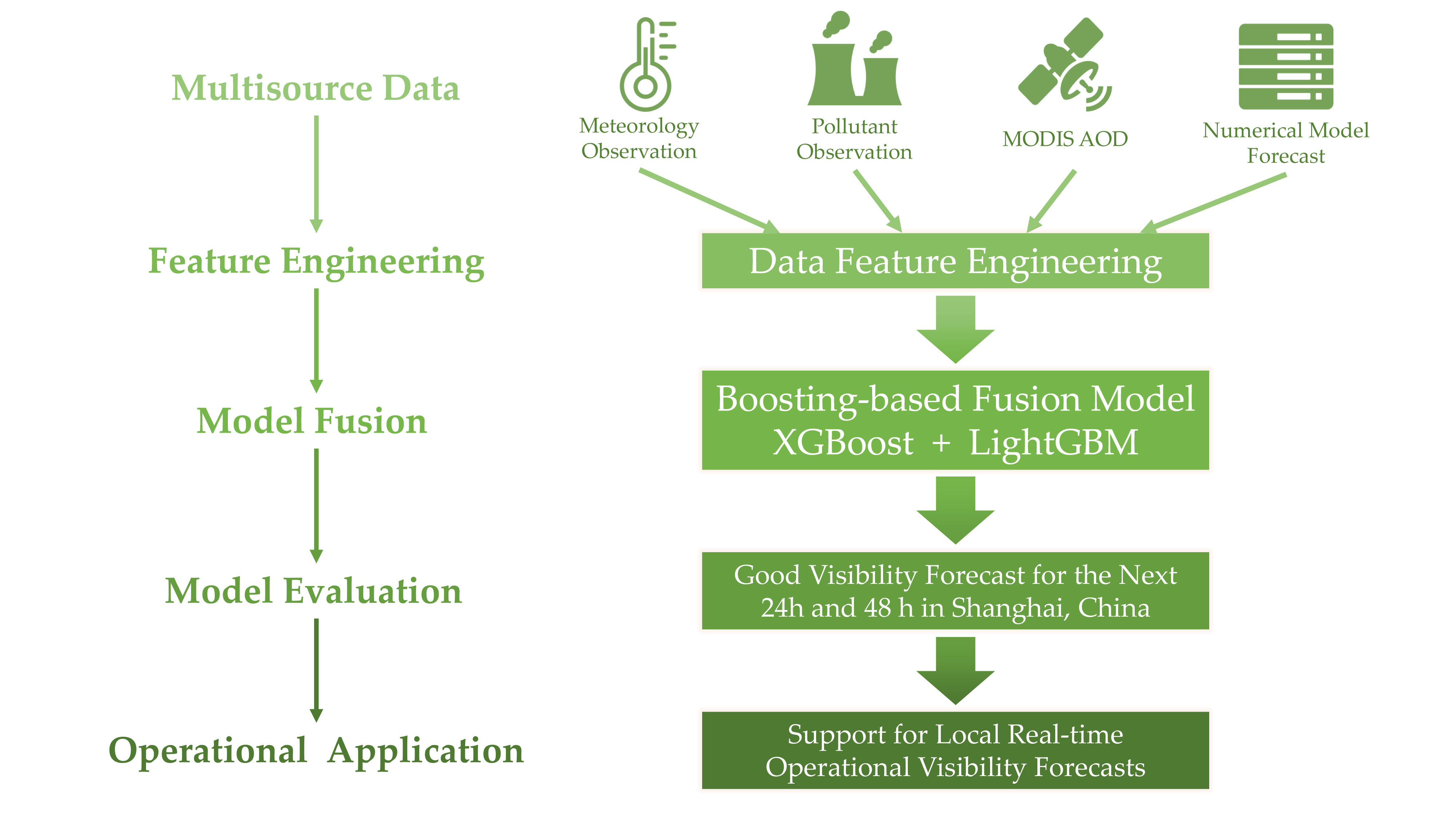
In this study, machine-learning-based model fusion was conducted using two models, XGBoost and LightGBM. These two boosting models can convert weak base classifiers into strong classifiers. First, an original dataset is trained to obtain a weak classifier. Then, the distribution of the new dataset is adjusted based on the performance of this weak classifier, allowing the incorrect training samples to receive more attention during the follow-up training process. Third, the adjusted sample data distribution is used for the next round of training to obtain the next weak classifier. We obtained several base weak classifiers after training for several rounds and combined these classifiers to build the final classifier. Single weak classifiers may not perform well, although the final classifier exhibits a good performance. In addition, XGBoost implements a general tree-boosting algorithm. It adds Lasso (L1) [52] or Ridge (L2) [53] regulation to avoid an over-fitting, uses the second derivative information of the cost function, and introduces the idea of column sampling, as compared with GBDT. XGBoost significantly improves the efficiency and generalization of the prediction model. For example, this algorithm has been applied to the estimation of PM2.5, which is highly correlated with visibility, and has shown a better performance than some other statistical and machine learning models [54,55,56]. LightGBM is a tree-based gradient-boosting framework. It was developed for distribution and shows a good performance in terms of both efficiency and memory consumption. This algorithm has also proven to be effective and acceptable in PM2.5 and visibility studies [33,57]. The framework of the machine-learning-based model fusion using XGBoost and LightGBM in this study is shown in Figure 2.
2.3.1. Feature Extraction
The model feature extraction was divided into three sections: basic, spatial, and temporal. To predict the visibility at one station, the basic features of the model included the observed meteorological and environmental variables, as well as the daily RAEMS predicted surface and high-altitude variables, as introduced in Section 2.1. For the spatial features, because the distribution of the variables at different altitudes presents the vertical movement and convection of the atmosphere, the differences between the same variable at different altitudes were calculated as new features representing the gradient change in the atmosphere in the vertical direction. In addition, considering horizontal atmospheric movement and correlation, important features at the four nearest stations were collected to predict the visibility at one station. For the temporal features, the differences between variables at adjacent moments 24 h before the initial forecast time were new features representing the tendencies of visibility and other related variables. To represent the regulation of visibility during recent periods, the previous 24, 48, 72, and 96 h visibility and related variables were also considered.
2.3.2. Data Sampling
Data from January 2015 to December 2018 were used as the training set for this visibility forecast, along with 385,377 data samples for 11 national synoptic stations, among which 327 data (0.08%) were missing. Five visibility levels were used to determine the visibility distribution (Table 1). Over half of the visibility hours exceeded 10 km. Compared to this high visibility, low visibility, which was below 5 km, only accounted for 23.4% of the entire period. In fact, the public is more concerned with the accuracy of low visibility forecast because it may result in discomfort or even meteorological disasters. To improve the accuracy of low-visibility prediction, the synthetic minority oversampling technique (SMOTE) was used in this study to adjust the training set and eliminate the influence of an imbalanced data distribution.
SMOTE [58] generates virtual training data for the minority class based on linear interpolation (k-nearest neighbor). For each data sample in the minority class, one or more k-nearest neighbors are randomly selected to build a virtual dataset for training. After the oversampling process, several classification methods are applied to process the new dataset. In this study, after applying the SMOTE process, the number of data points in the training set increased from 385,377 to 1,033,085 (approximately 93,916 for each synoptic station), and the number of data points for each visibility level was equivalent. The new training set was used for the formal training and forecasting. A 10-fold cross-verification [59,60] was also applied in this study to ensure not only the randomness of the verification set but also the similarity between the verification and training set checks. According to the verification results, the model was adjusted to a suitable parameterization.
2.3.3. Loss Function Adjustment
The training set was pre-processed and prepared as described in Section 2.3.1 and Section 2.3.2. Another important step used to conduct model fusing is to set different prediction tasks based on the loss function. The loss function is the mean square error (MSE), which is given by Equation (1):
where N refers to the sample numbers, and yi and oi refer to the forecasted value and the real value of the ith sample, respectively.
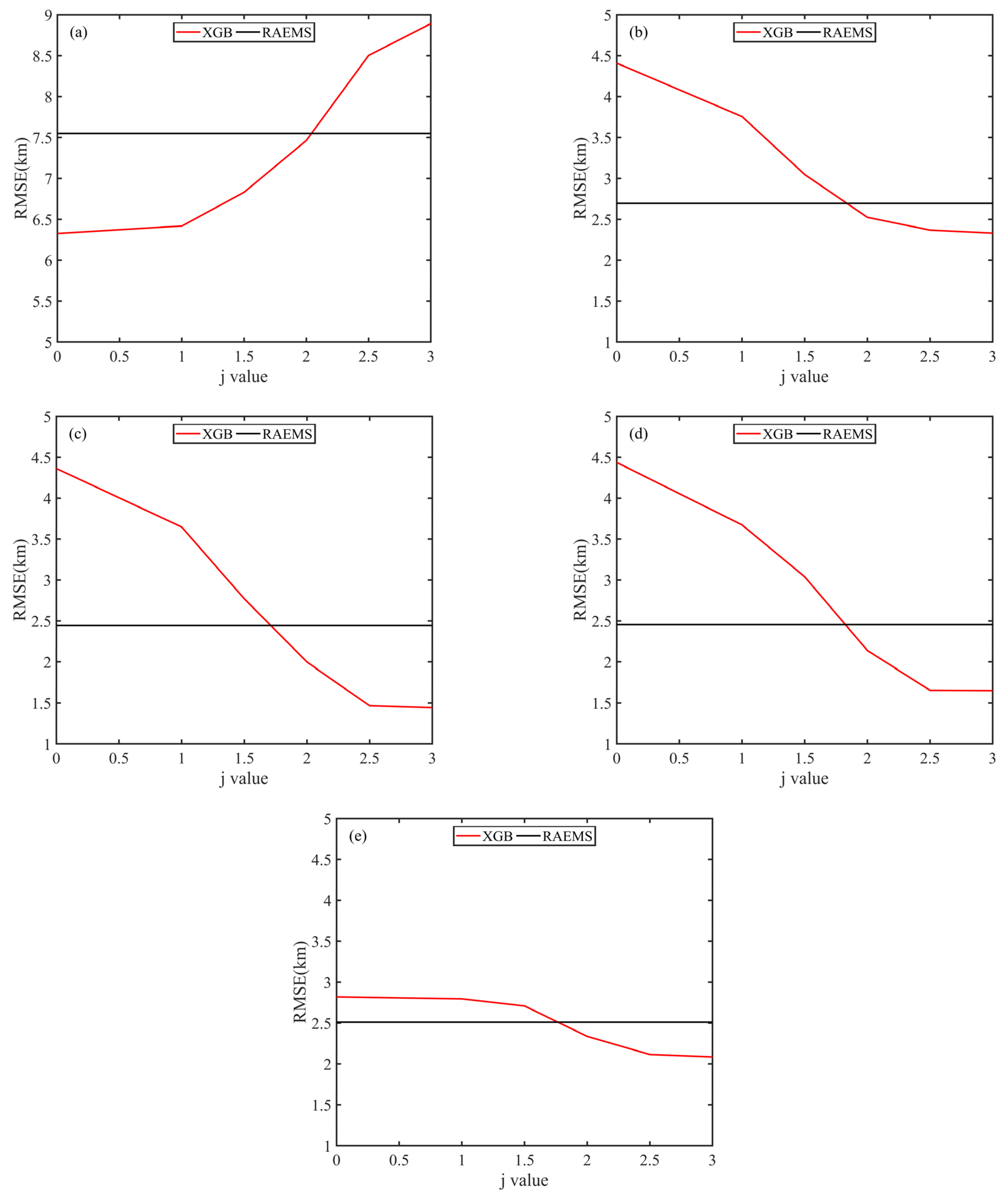
Considering the importance of the low visibility forecast, we adjusted the loss function and applied it to Equation (2):
where j is a constant. Different values of j represent a different emphasis on low visibility. With an increase in j, the root mean square error (RMSE) of the predicted low visibility decreased, whereas the RMSE of the entire range of visibility prediction increased. Taking a 24 h prediction as the adjustment example (Figure 3), when j = 2, the RMSEs of the XGBoost prediction and the RAEMS prediction were close to each other. For low-visibility situations, the RMSE of the XGBoost prediction was significantly smaller than that of the RAEMS prediction. Therefore, to obtain the best adjustment for low-visibility prediction in this study, j = 2 was used.
A binary classification used to judge whether the predicted visibility was greater than 10 km was conducted based on the loss function adjustment. This step considers the accuracy of both high- and low-visibility forecasts. If the predicted visibility was greater than 10 km, we used the high visibility prediction model (j = 0); otherwise, we used the low-visibility prediction model (j = 2). Using binary classification and model fusion, the RMSEs of the optimized XGBoost model (O-XGB) were significantly smaller than those of the other situations (Table 2).
2.3.4. Model Fusion
XGBoost and LightGBM were merged to build a new prediction model, the boosting-based fusion model (BFM). The normalized mean bias (NMB) and mean error (ME) were used as the moving weights for model merging [61]. First, we calculated the NMBs of XGBoost and LightGBM for the period prior to prediction (Equation (3)), where k denotes the two boosting models XGBoost and LightGBM, Nd is the number of days before prediction, yk,i and oi refer to the forecasted and real values of the ith sample, respectively. In this study, Nd equals to 10 days, which was reasonable after an evaluation of the number of days from 1 to 30. MEk denotes the mean bias of the modified forecast value (Equation (4)). Wk denotes the prediction weight for each model (Equation (5)), where Nm is the number of models (Nm = 2). Moreover, FF is the final prediction (Equation (6)). Four tasks, that is, high- and low-visibility prediction using XGBoost and LightGBM, respectively, were conducted. The different advantages of XGBoost and LightGBM are expected to improve the performance of the final model. For the testing data from 2019, the XGBoost and LightGBM models started forecasting at 6:00 a.m. each day. Thus, the 24 and 48 h forecasts in this study referred to the forecast visibility for every hour from 6:00 a.m. on the first day to 5:00 a.m. on the second day, and from 6:00 a.m. on the second day to 5:00 a.m. on the third day.
2.4. Statistical Scores
To quantitatively evaluate the accuracy of the forecast, the mean bias (MB), mean absolute error (MAE), mean relative error (MRE), root mean square error (RMSE), correlation coefficient (CC), 25% percentile, 75% percentile, median, and mean values were calculated. The calculations of MB, MAE, MRE, RMSE, and CC are shown in Equations (7)–(11), respectively:
where N is the number of samples, and yi and oi refer to the forecasted and real values of the ith sample, respectively.
3. Results
3.1. A Case Study Evaluation
In this section, to study the forecast performance of these three models, the average forecasts for the next 24 and 48 h in Shanghai city using the BFM were analyzed and compared with the RAEMS and LGBM predictions (single LightGBM prediction based on RAEMS, LGBM). The case of 8 March to 13 March 2019 was applied because a significant fluctuation in visibility occurred during this period and the lowest visibility reached less than 1 km for over 7 h, which turned out to be an extremely low visibility event. Both the 24 and 48 h forecast results revealed that the LGBM tended to perform well but with less accuracy than the other models in terms of the low-visibility prediction (Figure 4). RAEMS performed quite well under low visibility, but not as well as the other models when the visibility was above 10 km. All three models reflected the variations in the observations over time. Specifically, the BFM showed the lowest RMSE within the entire range and a low visibility forecast for both 24 and 48 h periods. Because of the low accuracy of LGBM in a low-visibility forecast, MB and RMSE (OBS < 5 km) were the largest among the three models. Both LGBM and BFM had close correlation coefficients with the observations during this event. In addition, for the prediction of extremely low visibility at below 1 km during this period, none of these three models were able to correctly predict within the same range, which revealed the shortage of this forecast algorithm. Overall, the best performance in this case was achieved using the BFM (Table 3).
3.2. Forecast Evaluation
3.2.1. Overall City Evaluation
The city-averaged forecast results for Shanghai from the 2019 testing dataset are presented in Table 4. All three models showed smaller mean and median values compared with the observation, among which the BFM forecasted the closest values. For the 75th percentile, the LGBM forecast results were the closest to the observations. The best 24/48 h prediction performance was achieved by the BFM, with a mean bias of −0.83/−0.74 km, an RMSE of 5.01/5.47 km, an MB of 3.90/4.24 km, and an MRE of 36.12%/39.53% with an R of 0.80/0.77. With the valid increase in the forecast time, the RMSE, MAE, and MRE increased, whereas the MB and CC decreased. For the low-level visibility forecast (for the three scenarios, [0, 5 km), [0, 3 km], and [0, 1 km]), the MB and RMSE of the three models were calculated. Under all scenarios, the BFM forecasted with the least mean bias and root mean square error. The mean bias when the visibility was under 5 km were 0.68 km for a 24 h forecast and 0.95 km for a 48 h forecast, which were both significantly smaller than in the other two models.
To analyze the error source, the RMSEs and MREs of the hourly prediction results for the next 24 h were calculated and compared (Figure 5). From the viewpoint of the RMSE variation over time, the RMSE of BFM was less than those of RAEMS and LGBM most of the time. After the third forecast hour, the RMSE of the three models increased dramatically and then fluctuated. There were two decreasing trends, from the 5th to the 10th forecast hour (11:00 a.m. to 16 p.m.) and from the 13th to the 22nd forecast hour (19:00 p.m. to 3 a.m. the next day). Both the BFM and LGBM reduced the RMSE and MAE of RAEMS. The smallest MRE of the three models appeared at the 8th forecast hour, which was at 13:00 in the afternoon, whereas the largest MRE appeared at the 22nd forecast hour, which was at 3:00 in the morning. These typical statistical results showed differences between the daytime and nighttime forecasts. During the daytime, particularly in the afternoon, the RMSE and MRE decreased to a relatively low level, whereas during the nighttime, they increased to a higher level. The results were in accord with those of a previous study [62].
In addition, because the BFM and LGBM predictions were both based on RAEMS-forecasted data, the error of RAEMS had a direct influence on the accuracy of the machine learning models. If the errors of RAEMS were large or had high randomness, XGBoost and LGBM would not recognize such errors, leading to a decrease in the accuracy of the visibility forecast. In this study, the two most dominant factors were the errors of the surface PM2.5 and the relative humidity from RAEMS. The correlation coefficient between the two above factors and the BFM forecasted visibility error were −0.39 and −0.45, respectively.
3.2.2. Station Evaluation
To evaluate the model error over Shanghai occurring from geographic differences, forecasts at Chongming (island station), Xujiahui (urban station), and Qingpu (suburban station) were investigated. Three typical synoptic stations are shown in Figure 5. Chongming Station is located on Chongming Island, north of Shanghai. Xujiahui is the core urban area of Shanghai. Qingpu is an inland suburban area located west of Shanghai. Statistics of 24 h forecast using RAEMS, BFM, and LGBM were illustrated to identify the detailed differences among the different model algorithms and different areas (Figure 6 and Table 5). Figure 6 indicates that BFM and LGBM improved the prediction to a large extent. The distribution of BFM revealed the advantages of RAEMS (25th percentile) and LGBM (median and 75th percentile). The comparison also focused on MB, RMSE, MAE, MRE, and CC between the observed and predicted visibility. The 24 and 48 h predictions of BFM and LGBM had a strong linear correlation (greater than 0.5) with the observed visibility at all three stations, which was more than 0.1 higher than that of RAEMS. All mean biases for the three stations were negative, which means that the average prediction underestimated the observation. The statistical indexes including RMSE, MAE, and MRE for the three stations showed that those of BFM were the smallest, whereas those of RAEMS were the largest. For Xujiahui Station, the predicted RMSE of RAEMS reached over 10 km, but with a significant improvement by the BFM to 4.32 km (24 h) and 5.69 km (48 h). A smaller MAE and MRE also appeared at Xujiahui and Qingpu, as compared with Chongming. Along with the fact that the observed visibility of Chongming had a larger deviation than the other inland stations, it was more difficult to achieve a similar forecast performance for the island areas than for the inland areas.
Another approach to assessing the models is to calculate the scores for the forecasted visibility of the model, regardless of visibility. In this section, low visibility was defined as less than 5 km. Frequency bias (FB), percent correct (PC), probability of omission (PO), probability of detection (POD), false alarm ratio (FAR), critical success index (CSI), and equitable threat score (ETS) were used to assess the performance of low-visibility forecasts. The algorithm details were recorded in a document titled ‘Guidelines on Performance Assessment of Public Weather Services (WMO/TD No. 1023)’ [63]. According to the score results listed in Table 6, in the island area (Chongming), the BFM had higher FB, POD, and FAR values than the other two models, but with the lowest PO, which indicated a slight over-forecasting of low visibility. The BFM had the highest CSI, whereas LGBM had the highest ETS. In the central urban area (Xujiahui), RAEMS and BFM shared the same PO (0.36) and POD (0.64), which indicates that these two models performed similarly in low-visibility forecasts. However, with a higher FB and FAR, RAEMS obtained a lower CSI and ETS than the BFM. In the inland suburb area (Qingpu), although the BFM had the highest FAR, its CSI and ETS were both the highest among the three models. When comparing the forecasts for the three areas, the ETS of RAEMS, BFM, and LGBM were 0.29, 0.33, and 0.29, respectively, for the forecasting visibility in the suburban area (Qingpu), which were all higher than those in urban and island areas, as were the CSI values. These results prove that low visibility in the island area was more difficult to predict from another perspective. In total, the binary score results were acceptable. It was concluded that BFM outperformed RAEMS and LGBM with a high correlation and the lowest error over Shanghai.
4. Discussion
Owing to the rapid increase of meteorological and environmental observational and numerical modeling data in recent years, researchers all over the world are engaging to use machine learning algorithms to conduct local visibility forecast. Many previous works used single algorithms to conduct visibility forecast at single stations and produced high quality results [28,29,30]. In accordance with the studies of Bari and Ouagabi [62] and Caruana and Niculescu-Mizil [64], where XGBoost and LightGBM ranked the top two algorithms among several single linear regression and machine learning methods in visibility forecasts, these two tree-based algorithms were chosen to conduct our prediction tasks. In our study, the correlation coefficient of BFM and LGBM reached 0.8, which was close to the results of Bari and Ouagabi. In fact, the model fusion prediction performed better. Zhang et al. [33] used a machine-learning-based multimodal fusion by combining surface and satellite atmospheric observations to predict the visibility within the Beijing-Tianjin-Hebei region. Similar to their study, both of our approaches used suitable surface and satellite observational data and showed that the RMSE of model fusion was significantly better than any single machine learning method or numerical model, which means that model fusion can significantly improve the local forecast capability. Moreover, the RMSEs of our BFM and LGBM predictions were both less than 6 km, which is smaller than that of Zhang et al.’s fused model prediction (6.71 km). The application of a numerical model system (RAEMS) and different geographic and environmental conditions may be important factors contributing to the lower prediction RMSEs and errors.
In fact, the accuracy of visibility forecasting is a problem in Shanghai, China. Researchers and forecasters have focused to use numerical models to study and predict haze/fog or air quality (PM2.5 and PM10) in Shanghai [8,65,66]. Zhou et al. [65] found detailed criteria for low visibility based on single variables including PM2.5, PM10, relative humidity, and wind speed. Zhou et al. [8] also used RAEMS to predict PM2.5 and PM10, which were well forecasted. In addition, Wang et al. [66] investigated that the correlation coefficient between daily observations and regional numerical model predictions based on RAEMS in Shanghai was 0.534 for the entire year from January to December. Compared with these previous studies, our work improved visibility prediction in Shanghai, which revealed an encouraging prospect of using machine-learning based model fusion to conduct visibility forecasts.
The model fusion method has several advantages. First, this method can capture forecast features from the RAEMS numerical modeling and historical observational features from observational stations and MODIS AOD products. It combines numerical modeling and machine learning to enhance the hourly forecast accuracy. Second, it includes a moving weight algorithm while merging XGBoost and LightGBM, thereby applying the best performances of these two boosting methods. Third, the results of this method demonstrate a reliable and effective way to spread to operational visibility forecasts in Shanghai.
Although this study successfully applied machine learning approaches to predict the visibility in Shanghai, certain limitations should be considered. First, as mentioned in Section 3.2.1, the forecast error of WRF-Chem-based RAEMS contributed to the BFM forecast and limited the final accuracy. Second, the model fusion-based machine learning model indicated different forecast effects when applied to individual stations in different areas of Shanghai; thus, there were some limitations in spatial representation. Third, there were many modeling and testing periods in this study, and the stability of the conclusions might have some limitations, which would be further optimized and revised in the future. Eventually, applying other deep learning algorithms, building ensemble forecast techniques, and improving the current machine learning algorithms will increase the accuracy of the visibility forecasting.
5. Conclusions
A BFM model for visibility prediction using a machine-learning-based model fusion based on multisource data, including RAEMS outputs, air pollutants, meteorological observations, and MODIS AOD data, was established in this study. Machine learning methods (XGBoost and LightGBM) and the numerical prediction method RAEMS were fused to build this prediction model. Three sets of prediction models, BFM, LightGBM based on multisource data (LGBM), and RAEMS were used to conduct prediction tasks. The prediction models were constructed based on the training set from 1 January 2015 to 31 December 2018 after several effective data pre-processing steps, including SMOTE data resampling, a loss function adjustment, and a 10-fold cross verification. Moreover, apart from the basic features (variables), more spatial and temporal gradient features were considered. A test set (from 1 January 2019 to 31 December 2019) was adopted to validate the feasibility of the BFM, RAEMS, and LGBM approaches. Statistical indicators including MB, MAE, MRE, RMSE, and CC confirmed that the machine learning methods improved the RAEMS forecast significantly and consistently. The correlation coefficient and root mean square error of BFM for the next 24/48 h periods were 0.80/0.77, and 5.01/5.47 km, respectively, which are much higher than those of RAEMS. The statistics and binary score analysis for different areas in Shanghai also proved the reliability and accuracy of using BFM, particularly in low-visibility forecasting. Overall, the BFM is a suitable tool for predicting visibility. It provides a more accurate visibility forecast for the next 24 and 48 h periods than LGBM and RAEMS in Shanghai. The results of this study provide support for real-time operational visibility forecasts.
Author Contributions
Conceptualization, Z.Y. and J.M.; methodology, Z.Y.; software, Z.Y. and Y.Q.; validation, Z.Y., Y.W., and Y.C.; formal analysis, Y.Q. and Y.W.; investigation, J.M. and Y.C.; resources, Y.C.; data curation, Z.Y. and Y.Q.; writing—original draft preparation, Z.Y.; writing—review and editing, Z.Y., J.M., and Y.Q.; visualization, Z.Y.; supervision, J.M.; project administration, Z.Y.; funding acquisition, Z.Y. and J.M. All authors have read and agreed to the published version of the manuscript.
Funding
This research was funded by the Chinese Ministry of Science and Technology (Grant No. 2019YFC0214605), the National Natural Science Foundation of China (Grant No. 42005055, 91644223, and 41475040), the Natural Science Foundation of Shanghai (Grant No. 19ZR1462100), and the Shanghai Science and Technology Commission (Grant No. 19DZ1205003).
Institutional Review Board Statement
Not applicable.
Informed Consent Statement
Not applicable.
Data Availability Statement
The data presented in this study are available on request from the corresponding author.
Acknowledgments
We are grateful to our colleagues at Shanghai Meteorological Service for their help and input, without which this study would not have been possible.
Conflicts of Interest
The authors declare no conflict of interest. The funders had no role in the design of the study; in the collection, analyses, or interpretation of data; in the writing of the manuscript; or in the decision to publish the results.
References
- Horvath, H. Atmospheric visibility. Atmos. Environ. 1981, 15, 1785–1796. [Google Scholar] [CrossRef]
- Deng, X.; Tie, X.; Wu, D.; Zhou, X.; Bi, X.; Tan, H.; Li, F.; Jiang, C. Long-term trend of visibility and its characterizations in the Pearl River Delta (PRD) region, China. Atmos. Environ. 2008, 42, 1424–1435. [Google Scholar] [CrossRef]
- Qian, W.; Leung, J.C.-H.; Chen, Y.; Huang, S. Applying anomaly-based weather analysis to the prediction of low visibility associated with the coastal fog at Ningbo-Zhoushan Port in East China. Adv. Atmos. Sci. 2019, 36, 1060–1077. [Google Scholar] [CrossRef] [Green Version]
- Gultepe, I.; Sharman, R.; Williams, P.D.; Zhou, B.; Ellrod, G.; Minnis, P.; Trier, S.; Griffin, S.; Yum, S.S.; Gharabaghi, B.; et al. A review of high impact weather for aviation meteorology. Pure Appl. Geo-Phys. 2019, 176, 1869–1921. [Google Scholar] [CrossRef]
- Cheung, K.; Daher, N.; Kam, W.; Shafer, M.; Ning, Z.; Schauer, J.; Sioutas, C. Spatial and temporal variation of chemical composition and mass closure of ambient coarse particulate matter (PM10–2.5) in the Los Angeles area. Atmos. Environ. 2011, 45, 2651–2662. [Google Scholar] [CrossRef]
- Hu, Y.; Yao, L.; Cheng, Z.; Wang, Y. Long-term atmospheric visibility trends in megacities of China, India and the United States. Environ. Res. 2017, 159, 466–473. [Google Scholar] [CrossRef]
- Grell, G.A.; Peckham, S.E.; Schmitz, R.; McKeen, S.A.; Frost, G.; Skamarock, W.C.; Eder, B. Fully coupled ’online’ chemistry in the WRF model. Atmos. Environ. 2005, 39, 6957–6976. [Google Scholar] [CrossRef]
- Zhou, G.; Xu, J.; Xie, Y.; Chang, L.; Gao, W.; Gu, Y.; Zhou, J. Numerical air quality forecasting over eastern China: An operational application of WRF-Chem. Atmos. Environ. 2017, 153, 94–108. [Google Scholar] [CrossRef]
- Binkowski, F.S.; Roselle, S.J. Models-3 community multiscale air quality (cmaq) model aerosol component 1. model description. J. Geophys. Res. Atmos. 2003, 108, 4183. [Google Scholar] [CrossRef]
- Cheng, F.; Feng, C.; Yang, Z.; Hsu, C.; Chan, K.; Lee, C.; Chang, S. Evaluation of real-time PM2.5 forecasts with the WRF-CMAQ modeling system and weather-pattern-dependent bias-adjusted PM2.5 forecasts in Taiwan. Atmos. Environ. 2020, 244. [Google Scholar] [CrossRef]
- An, X.; Zhai, S.; Jin, M.; Gong, S.; Wang, Y. Development of an adjoint model of GRAPES–CUACE and its application in tracking influential haze source areas in north China. Geosci. Model Dev. 2016, 9, 2153–2165. [Google Scholar] [CrossRef]
- Yumimoto, K.; Uno, I. Adjoint inverse modeling of CO emissions over Eastern Asia using four-dimensional variational data assimilation. Atmos. Environ. 2006, 40, 6836–6845. [Google Scholar] [CrossRef]
- Yang, D.; Ritchie, H.; Desjardins, S.; Pearson, G.; MacAfee, A.; Gultepe, I. High-resolution GEM-LAM application in marine fog prediction: Evaluation and diagnosis. Weather Forecast. 2010, 25, 727–748. [Google Scholar] [CrossRef]
- Duynkerke, P.G. Radiation fog: A comparison of model simulation with detailed observations. Mon. Weather Rev. 1991, 119, 324–341. [Google Scholar] [CrossRef] [Green Version]
- Guedalia, D.; Bergot, T. Numerical forecasting of radiation fog. Part II: A comparison of model simulation with several observed fog events. Mon. Weather Rev. 1994, 122, 1231–1246. [Google Scholar] [CrossRef] [Green Version]
- Makridakis, S.; Spiliotis, E.; Assimakopoulos, V. Statistical and Machine Learning forecasting methods: Concerns and ways forward. PLoS ONE. 2018, 13, e0194889. [Google Scholar] [CrossRef] [Green Version]
- Zhang, G.; Eddy Patuwo, B.; Hu, Y. Forecasting with artificial neural networks: The state of the art. Int. J. Forecast. 1998, 14, 35–62. [Google Scholar] [CrossRef]
- Xiao, Q.; Chang, H.H.; Geng, G.; Liu, Y. An ensemble machine-learning model to predict historical PM2.5 concentrations in China from satellite data. Environ. Sci. Technol. 2018, 52, 13260–13269. [Google Scholar] [CrossRef] [PubMed]
- Xu, Y.; Ho, H.C.; Wong, M.S.; Deng, C.; Shi, Y.; Chan, T.-C.; Knudby, A. Evaluation of machine learning techniques with multiple remote sensing datasets in estimating monthly concentrations of ground-level PM2.5. Environ. Pollut. 2018, 242, 1417–1426. [Google Scholar] [CrossRef] [PubMed]
- Cecaj, A.; Lippi, M.; Mamei, M.; Zambonelli, F. Comparing deep learning and statistical methods in forecasting crowd distribution from aggregated mobile phone data. Appl. Sci. 2020, 10, 6580. [Google Scholar] [CrossRef]
- Wei, C.C.; Hsieh, P.Y. Estimation of hourly rainfall during typhoons using radar mosaic-based convolutional neural networks. Remote Sens. 2020, 12, 896. [Google Scholar] [CrossRef] [Green Version]
- Bouget, V.; Béréziat, D.; Brajard, J.; Charantonis, A.; Filoche, A. Fusion of rain radar images and wind forecasts in a deep learning model applied to rain nowcasting. Remote Sens. 2021, 13, 246. [Google Scholar] [CrossRef]
- Kianian, B.; Liu, Y.; Chang, H. Imputing satellite-derived aerosol optical depth using a multi-resolution spatial model and random forest for PM2.5 prediction. Remote Sens. 2021, 13, 126. [Google Scholar] [CrossRef]
- Fan, Z.; Zhan, Q.; Yang, C.; Liu, H.; Bilal, M. Estimating PM2.5 concentrations using spatially local xgboost based on full-covered SARA AOD at the urban scale. Remote Sens. 2020, 12, 3368. [Google Scholar] [CrossRef]
- Wei, J.; Li, Z.; Lyapustin, A.; Sun, L.; Peng, Y.; Xue, W.; Su, T.; Cribb, M. Reconstructing 1-km-resolution high-quality PM2.5 data records from 2000 to 2018 in China: Spatiotemporal variations and policy implications. Remote Sens. Environ. 2021, 252, 112136. [Google Scholar] [CrossRef]
- Wei, J.; Li, Z.; Xue, W.; Sun, L.; Fan, T.; Liu, L.; Su, T.; Cribb, M. The ChinaHighPM10 dataset: Generation, validation, and spatiotemporal variations from 2015 to 2019 across China. Environ. Int. 2021, 146, 106290. [Google Scholar] [CrossRef]
- Su, T.; Laszlo, I.; Li, Z.; Wei, J.; Kalluri, S. Refining aerosol optical depth retrievals over land by constructing the relationship of spectral surface reflectances through deep learning: Application to Himawari-8. Remote Sens. Environ. 2020, 251, 112093. [Google Scholar] [CrossRef]
- Bari, D.; El Khlifi, M. LVP conditions at Mohamed V airport, Morocco: Local characteristics and prediction using neural networks. Int. J. Basic. Appl. Sci. 2015, 4, 354–363. [Google Scholar] [CrossRef] [Green Version]
- Marzban, C.; Leyton, S.; Colman, B. Ceiling and visibility forecasts via neural networks. Weather Forecast. 2007, 22, 466–479. [Google Scholar] [CrossRef] [Green Version]
- Bartoková, I.; Bott, A.; Bartok, J.; Gera, M. Fog prediction for road traffic safety in a coastal desert region: Improvement of nowcasting skills by the machine-learning approach. Boundary-Layer Meteorol. 2015, 157, 501–51617. [Google Scholar] [CrossRef]
- Glahn, B.; Schnapp, A.D.; Ghirardelli, J.E.; Im, J.S. A LAMP-HRRR Meld for improved aviation guidance. Weather Forecast. 2017, 32, 391–405. [Google Scholar] [CrossRef]
- Jiang, F.; Yu, X.; Du, J.; Gong, D.; Zhang, Y.; Peng, Y. Ensemble learning based on approximate reducts and bootstrap sampling. Inform. Sci. 2020, 547, 797–813. [Google Scholar] [CrossRef]
- Zhang, C.; Wu, M.; Chen, J.; Chen, K.; Zhang, C.; Xie, C.; Huang, B.; He, Z.C. Weather visibility prediction based on multimodal fusion. IEEE Access 2019, 7, 74776–74786. [Google Scholar] [CrossRef]
- Berger, A.; Pietra, S.D.; Pietra, V.D. A maximum entropy approach to natural language processing. Comput. Linguist. 1996, 22, 39–71. Available online: https://www.aclweb.org/anthology/J96-1002/ (accessed on 9 May 2020).
- Platt, J.C. Sequential Minimal Optimization: A Fast Algorithm for Training Support Vector Machines; Technical Report MSR-TR-98-14; Microsoft Research: Redmond, WA, USA, 1998. [Google Scholar]
- Schapire, R.E. A brief introduction to boosting. In Proceedings of the 16th International Joint Conference on Artificial Intelligence, Stockholm, Sweden, 31 July–6 August 1999; Volume 99, pp. 1401–1406. [Google Scholar]
- Breiman, L. Bagging predictors. Mach. Learn. 1996, 24, 123–140. [Google Scholar] [CrossRef] [Green Version]
- Freund, Y.; Schapire, R.E. A decision-theoretic generalization of on-line learning and an application to boosting. J. Comput. Syst. Sci. 1997, 55, 119–139. [Google Scholar] [CrossRef] [Green Version]
- Friedman, J.H. Greedy Function Approximation: A Gradient Boosting Machine. Ann Stat. 2001, 29, 1189–1232. [Google Scholar] [CrossRef]
- Chen, T.; Guestrin, C. XGBoost: A Scalable Tree Boosting System. In Proceedings of the 22nd Acm Sigkdd International Conference on Knowledge Discovery and Data Mining, San Francisco, CA, USA, 13–17 August 2016; pp. 785–794. [Google Scholar]
- Ke, G.; Meng, Q.; Finley, T.; Wang, T.; Chen, W.; Ma, W.; Ye, Q.; Liu, T. LightGBM: A highly efficient gradient boosting decision tree. In Proceedings of the 31st Annual Conference on Neural Information Processing Systems, Long Beach, CA, USA, 4–9 December 2017; pp. 3146–3154. [Google Scholar]
- Prokhorenkova, L.; Gusev, G.; Vorobev, A.; Dorogush, A.V.; Gulin, A. CatBoost: Unbiased boosting with categorical features. In Proceedings of the 32nd Annual Conference on Neural Information Processing Systems, Montreal, QC, Canada, 3–8 December 2018; pp. 6637–6647. [Google Scholar]
- Breiman, L. Random Forests. Mach. Learn. 2001, 45, 5–32. [Google Scholar] [CrossRef] [Green Version]
- Dietterich, T.G. An experimental comparison of three methods for constructing ensembles of decision trees: Bagging, boosting, and randomization. Mach. Learn. 2000, 40, 139–157. [Google Scholar] [CrossRef]
- Feng, L.; Li, Y.; Wang, Y.; Du, Q. Estimating hourly and continuous ground-level PM2.5 concentrations using an ensemble learning algorithm: The ST-stacking model. Atmos. Environ. 2020, 223, 117242. [Google Scholar] [CrossRef]
- Lee, J.; Wang, W.; Harrou, F.; Sun, Y. Reliable solar irradiance prediction using ensemble learning-based models: A comparative study. Energ Convers. Manag. 2020, 208, 112582. [Google Scholar] [CrossRef] [Green Version]
- Lyapustin, A.; Wang, Y. MCD19A2 MODIS/Terra+Aqua Land Aerosol Optical Depth Daily L2G Global 1km SIN Grid V006. 2018. Distributed by NASA EOSDIS Land Processes DAAC. Available online: https://0-doi-org.brum.beds.ac.uk/10.5067/MODIS/MCD19A2.006 (accessed on 9 May 2020).
- Lyapustin, A.; Martonchik, J.; Wang, Y.; Laszlo, I.; Korkin, S. Multi-Angle Implementation of Atmospheric Correction (MAIAC): 1. Radiative transfer basis and look-up tables. J. Geophys. Res. Atmos. 2011, 116, D03210. [Google Scholar] [CrossRef]
- Lyapustin, A.; Wang, Y.; Laszlo, I.; Kahn, R.; Korkin, S.; Remer, L.; Levy, R.; Reid, J.S. Multi-Angle Implementation of Atmospheric Correction (MAIAC): 2. Aerosol algorithm. J. Geophys. Res. Atmos. 2011, 116, D03211. [Google Scholar] [CrossRef]
- Lyapustin, A.; Wang, Y.; Laszlo, I.; Hilker, T.; Hall, F.; Sellers, P.; Tucker, C.; Korkin, S. Multi-Angle Implementation of Atmospheric Correction (MAIAC): 3. Atmospheric correction. Remote Sens. Environ. 2012, 127, 385–393. [Google Scholar] [CrossRef]
- Wei, J.; Huang, W.; Li, Z.; Xue, W.; Peng, Y.; Sun, L.; Cribb, M. Estimating 1-km-resolution PM2. 5 concentrations across China using the space-time random forest approach. Remote Sens. Environ. 2019, 231, 111221. [Google Scholar] [CrossRef]
- Tibshirani, R. Regression shrinkage and selection via the lasso. J. R. Stat. Soc. B 1996, 58, 267–288. [Google Scholar] [CrossRef]
- Schreiber-Gregory, D.N. Ridge Regression and multicollinearity: An in-depth review. Model. Assist. Stat. Appl. 2018, 13, 359–365. [Google Scholar] [CrossRef] [Green Version]
- Ma, J.; Yu, Z.; Qu, Y.; Xu, J.; Cao, Y. Application of the XGBoost Machine Learning Method in PM2.5 Prediction: A Case Study of Shanghai. Aerosol Air Qual. Res. 2020, 20, 128–138. [Google Scholar] [CrossRef] [Green Version]
- Zhai, B.; Chen, J. Development of a stacked ensemble model for forecasting and analyzing daily average PM2.5 concentrations in Beijing, China. Sci. Total Environ. 2018, 635, 644–658. [Google Scholar] [CrossRef]
- Reid, C.E.; Jerrett, M.; Petersen, M.L.; Pfister, G.G.; Morefield, P.E.; Tager, I.B.; Raffuse, S.M.; Balmes, J.R. Spatiotemporal prediction of fine particulate matter during the 2008 Northern California wildfires using machine learning. Environ. Sci. Technol. 2015, 49, 3887–3896. [Google Scholar] [CrossRef]
- Zhong, J.; Zhang, X.; Gui, K.; Wang, Y.; Che, H.; Shen, X.; Zhang, L.; Zhang, Y.; Sun, J.; Zhang, W. Robust prediction of hourly PM2.5 from meteorological data using Light GBM. Natl. Sci. Rev. 2021, nwaa307. [Google Scholar] [CrossRef]
- Chawla, N.V.; Bowyer, K.W.; Hall, L.O.; Kegelmeyer, W.P. SMOTE: Synthetic minority over-sampling technique. J. Artif. Intell. Res. 2002, 16, 321–357. [Google Scholar] [CrossRef]
- Stone, M. Cross-validatory choice and assessment of statistical predictions. J. R. Stat. Soc. B Meteorol. 1974, 36, 111–147. [Google Scholar] [CrossRef]
- Rodriguez, J.D.; Perez, A.; Lozano, J.A. Sensitivity analysis of k-fold cross validation in prediction error estimation. IEEE Trans. Pattern Anal. Mach. Intell. 2010, 32, 569–575. [Google Scholar] [CrossRef] [PubMed]
- Woodcock, F.; Engel, C. Operational consensus forecasts. Weather Forecast. 2005, 20, 101–111. [Google Scholar] [CrossRef]
- Bari, D.; Ouagabi, A. Machine-learning regression applied to diagnose horizontal visibility from mesoscale NWP model forecasts. SN Appl. Sci. 2020, 2, 556. [Google Scholar] [CrossRef] [Green Version]
- Gordon, N.; Shaykewich, J. Guidelines on Performance Assessment of Public Weather Services; WMO/TD No. 1023; World Meteorological Organization: Geneva, Switzerland, 2000. [Google Scholar]
- Caruana, R.; Niculescu-Mizil, A. An empirical comparison of supervised learning algorithms. In Proceedings of the 23rd international conference on Machine-learning, Pittsburgh, PA, USA, 25–29 June 2006; pp. 161–168. [Google Scholar]
- Zhou, G.; Yang, F.; Geng, F.; Xu, J.; Yang, X.; Tie, X. Measuring and Modeling Aerosol: Relationship with Haze Events in Shanghai, China. Aerosol Air Qual. Res. 2014, 14, 783–792. [Google Scholar] [CrossRef] [Green Version]
- Wang, T.; Jiang, F.; Deng, J.; Shen, Y.; Fu, Q.; Wang, Q.; Fu, Y.; Xu, J.; Zhang, D. Urban air quality and regional haze weather forecast for Yangtze River Delta region. Atmos. Environ. 2012, 58, 70–83. [Google Scholar] [CrossRef]
Figure 1.
(a) Coverage of RAEMS (inside the red box); (b) locations of synoptic stations in Shanghai.
Figure 1.
(a) Coverage of RAEMS (inside the red box); (b) locations of synoptic stations in Shanghai.

Figure 2.
The framework of machine learning model fusion using XGBoost and LightGBM.

Figure 3.
Relationship between different ranges of visibility and j value: (a) [0, ∞); (b) [0, 10 km); (c) [0, 5 km); (d) [0, 3 km); (e) [0, 1 km).
Figure 3.
Relationship between different ranges of visibility and j value: (a) [0, ∞); (b) [0, 10 km); (c) [0, 5 km); (d) [0, 3 km); (e) [0, 1 km).

Figure 4.
Comparison between predictions of three models and the observations from 8 March to 13 March 2019: (a) 24 h prediction; (b) 48 h prediction.
Figure 4.
Comparison between predictions of three models and the observations from 8 March to 13 March 2019: (a) 24 h prediction; (b) 48 h prediction.


Figure 5.
Variation of (a) forecast RMSE and (b) MRE over time.

Figure 6.
Boxplots of the 24 h model forecast at three synoptic stations in Shanghai, i.e., (a) Chongming; (b) Xujiahui; (c) Qingpu.
Figure 6.
Boxplots of the 24 h model forecast at three synoptic stations in Shanghai, i.e., (a) Chongming; (b) Xujiahui; (c) Qingpu.


Table 1.
Sample percentage of different visibility levels.
| Range | [10 km, ∞) | [5 km, 10 km) | [3 km, 5 km) | [1 km, 3 km) | [0 km, 1 km) |
|---|---|---|---|---|---|
| Pieces | 206,617 | 88,766 | 46,042 | 38,570 | 5382 |
| Percentage | 53.6% | 23.0% | 12.0% | 10.0% | 1.4% |
Table 2.
The RMSEs of different models after a 10-fold cross verification.
| Visibility Range | [0 km, ∞) | [0 km, 10 km) | [0 km, 5 km) | [0 km, 3 km) | [0 km, 1 km) |
|---|---|---|---|---|---|
| XGBoost (j = 0) | 5.67 | 4.43 | 3.94 | 4.33 | 2.21 |
| XGBoost (j = 2) | 6.46 | 2.29 | 1.41 | 1.87 | 2.11 |
| O-XGB | 4.68 | 3.53 | 1.88 | 1.78 | 1.92 |
| RAEMS | 7.51 | 2.69 | 2.44 | 2.45 | 2.51 |
Table 3.
Statistics of visibility forecast evaluation in the case study based on different model techniques (RAEMS, LGBM, and BFM).
Table 3.
Statistics of visibility forecast evaluation in the case study based on different model techniques (RAEMS, LGBM, and BFM).
| Model | RMSE 24/48 h | MB 24/48 h | MAE 24/48 h | CC 24/48 h | RMSE (OBS < 5 km) 24/48 h |
|---|---|---|---|---|---|
| RAEMS | 5.34/5.23 | −0.13/−0.79 | 3.94/3.99 | 0.664/0.651 | 2.39/2.61 |
| LGBM | 2.83/2.91 | 1.890/1.10 | 2.42/2.29 | 0.952/0.921 | 3.23/3.41 |
| BFM | 2.25/2.63 | 0.20/−0.47 | 1.78/1.99 | 0.946/0.925 | 1.33/1.65 |
Unit: km. OBS refers to the observational visibility.
Table 4.
Visibility prediction (24/48 h) results.
| Observation | RAEMS | BFM | LGBM | |
|---|---|---|---|---|
| Mean value (km) | 13.14 | 7.99/7.71 | 12.23/12.32 | 10.56/10.41 |
| Median (km) | 11.43 | 7.27/6.95 | 11.30/11.43 | 10.15/10.05 |
| 25% percentile (km) | 6.05 | 5.14/4.99 | 4.80/4.65 | 7.48/7.71 |
| 75% percentile (km) | 19.74 | 10.10/9.66 | 15.89/15.55 | 16.26/16.16 |
| MB (km) | −5.15/−5.44 | −0.83/−0.74 | −2.51/−2.65 | |
| MB [0, 5 km) | 1.44/1.41 | 0.68/0.95 | 2.71/2.77 | |
| MB [0, 3 km) | 2.05/1.99 | 1.06/1.42 | 2.39/2.65 | |
| MB [0, 1 km) | 1.96/2.28 | 1.28/1.85 | 2.74/3.74 | |
| RMSE (km) | 8.45/8.86 | 5.01/5.47 | 5.45/5.88 | |
| RMSE [0, 5 km) | 2.52/2.37 | 2.28/2.63 | 2.89/3.66 | |
| RMSE [0, 3 km) | 2.75/2.64 | 1.89/2.56 | 2.68/2.87 | |
| RMSE [0, 1 km) | 2.00/2.34 | 1.38/2.04 | 2.42/3.11 | |
| MAE (km) | 6.29/6.60 | 3.90/4.24 | 4.06/4.38 | |
| MRE (%) | 48.04/49.56 | 36.12/39.53 | 45.09/51.33 | |
| CC | 0.58/0.52 | 0.80/0.77 | 0.80/0.75 |
Table 5.
Visibility prediction (24/48 h) results.
| Statistics | Station | RAEMS | BFM | LGBM |
|---|---|---|---|---|
| MB (km) | Chongming | −4.57/−4.91 | −1.95/−2.03 | −3.21/−2.60 |
| Xujiahui | −6.56/−6.82 | −1.28/−1.08 | −2.53/−2.60 | |
| Qingpu | −3.60/3.87 | −0.16/−0.08 | −1.98/−2.15 | |
| RMSE (km) | Chongming | 9.22/9.69 | 6.52/6.99 | 7.00/7.30 |
| Xujiahui | 10.04/10.37 | 4.32/5.69 | 6.19/6.72 | |
| Qingpu | 7.85/8.30 | 5.05/5.84 | 6.19/6.50 | |
| MAE (km) | Chongming | 6.91/7.23 | 5.73/6.10 | 6.30/6.74 |
| Xujiahui | 7.54/7.81 | 4.79/5.14 | 4.97/5.26 | |
| Qingpu | 5.60/5.93 | 4.44/4.78 | 4.48/4.72 | |
| MRE (%) | Chongming | 106.63/106.79 | 68.67/75.48 | 98.90/108.82 |
| Xujiahui | 52.85/54.04 | 44.75/47.42 | 51.64/56.39 | |
| Qingpu | 67.11/69.85 | 52.70/58.01 | 77.29/92.53 | |
| CC | Chongming | 0.54/0.48 | 0.77/0.71 | 0.69/0.59 |
| Xujiahui | 0.53/0.48 | 0.75/0.73 | 0.72/0.70 | |
| Qingpu | 0.60/0.58 | 0.75/0.74 | 0.76/0.71 |
Table 6.
Binary scores for the 24 h forecasts at the three synoptic stations in Shanghai (<5 km).
| Station | Model | FB | PC | PO | POD | FAR | CSI | ETS |
|---|---|---|---|---|---|---|---|---|
| Chongming | RAEMS | 0.70 | 0.79 | 0.60 | 0.40 | 0.43 | 0.31 | 0.21 |
| BFM | 1.98 | 0.70 | 0.13 | 0.87 | 0.56 | 0.41 | 0.24 | |
| LGBM | 0.73 | 0.80 | 0.54 | 0.46 | 0.38 | 0.35 | 0.26 | |
| Xujiahui | RAEMS | 1.93 | 0.72 | 0.36 | 0.64 | 0.67 | 0.28 | 0.16 |
| BFM | 1.52 | 0.79 | 0.36 | 0.64 | 0.58 | 0.34 | 0.24 | |
| LGBM | 0.56 | 0.83 | 0.72 | 0.28 | 0.50 | 0.22 | 0.16 | |
| Qingpu | RAEMS | 1.03 | 0.78 | 0.38 | 0.62 | 0.40 | 0.44 | 0.29 |
| BFM | 1.52 | 0.77 | 0.16 | 0.84 | 0.44 | 0.50 | 0.33 | |
| LGBM | 0.59 | 0.79 | 0.58 | 0.42 | 0.28 | 0.36 | 0.29 |
Publisher’s Note: MDPI stays neutral with regard to jurisdictional claims in published maps and institutional affiliations. |
© 2021 by the authors. Licensee MDPI, Basel, Switzerland. This article is an open access article distributed under the terms and conditions of the Creative Commons Attribution (CC BY) license (https://creativecommons.org/licenses/by/4.0/).
Share and Cite
MDPI and ACS Style
Yu, Z.; Qu, Y.; Wang, Y.; Ma, J.; Cao, Y. Application of Machine-Learning-Based Fusion Model in Visibility Forecast: A Case Study of Shanghai, China. Remote Sens. 2021, 13, 2096. https://0-doi-org.brum.beds.ac.uk/10.3390/rs13112096
AMA Style
Yu Z, Qu Y, Wang Y, Ma J, Cao Y. Application of Machine-Learning-Based Fusion Model in Visibility Forecast: A Case Study of Shanghai, China. Remote Sensing. 2021; 13(11):2096. https://0-doi-org.brum.beds.ac.uk/10.3390/rs13112096
Chicago/Turabian StyleYu, Zhongqi, Yuanhao Qu, Yunxin Wang, Jinghui Ma, and Yu Cao. 2021. "Application of Machine-Learning-Based Fusion Model in Visibility Forecast: A Case Study of Shanghai, China" Remote Sensing 13, no. 11: 2096. https://0-doi-org.brum.beds.ac.uk/10.3390/rs13112096
Note that from the first issue of 2016, this journal uses article numbers instead of page numbers. See further details here.