
Mapping Land Surface Temperature Developments in Functional Urban Areas across Europe


1
Federal Institute for Research on Building, Urban Affairs and Spatial Development (BBSR), 53179 Bonn, Germany
2
Institute of Geography, Ruhr University Bochum, 44780 Bochum, Germany
*
Author to whom correspondence should be addressed.
Remote Sens. 2021, 13(11), 2111; https://0-doi-org.brum.beds.ac.uk/10.3390/rs13112111
Submission received: 3 March 2021
/
Revised: 21 May 2021
/
Accepted: 25 May 2021
/
Published: 27 May 2021
(This article belongs to the Special Issue Application of Remote Sensing in Urban Climatology)
Abstract
:Unsustainable development paths have reached critical levels in Europe. In recent years, in cities, urbanization has been contributing to the intensification of urban heat islands. To analyze the development of surface urban heat islands (SUHI) in Europe in the last few years, the present study combines the land surface temperature (LST) from MODIS with the urban classes of the CORINE land cover data within 617 functional urban areas (FUAs). Urban and industrial uses have significantly higher LST than green urban areas across all years (about 4 to 6 °C), as do agricultural areas within cities. Besides land cover, location also influences LST differences. While, e.g., Bolzano (Italy) shows particularly large LST differences (>6 °C) between the core and the commuting zone, this effect is hardly visible in Porto (Portugal) and Madrid (Spain) (<2.5 °C). Cities of moderate climates show increasing differences between a city and its commuting zones with rising LST (r = 0.68), i.e., less cooling effects at night.
1. Introduction
Rising temperatures and more frequent heat waves caused by climate change have an increasing impact on our daily life [1]. The human body reacts to extreme air temperatures with increased sweating, falling blood pressure, and higher heart rates. If heat waves already represent an impairment in daily life for a healthy human organism, the consequences for physically vulnerable people, senior citizens, and children are many times higher and more dangerous [2]. In parallel with climate change, increasing heat stress is exacerbated by growing settlement pressure and advancing urbanization.
Both climate change and current demographic trends, as well as urban development, will lead to increased heat-related mortality and morbidity. The current demographic trends include both the ageing population [3] and migration to cities, particularly in northern and even central Europe [4]. The PESETA (Projection of Economic impacts of climate change in Sectors of the EU based on bottom-up Analysis) study forecasts about 90,000 deaths per year in the EU-27 member states and the UK in the period 2071–2100, with an average temperature increase of 3 °C, compared to 2700 annual deaths today [5]. According to Kemen et al. [6], heat extremes are therefore one of the greatest health challenges of climate change. The IPCC already described them in 2001: ‘Extreme weather episodes may lead to changes in deaths, injuries, or illness. For example, health status may improve as a result of reduced cold stress or deteriorate as a result of increased heat stress and disease’ [7].
The urban climate is particularly characterized by the fact that climatic conditions are heavily influenced by human beings. In addition to the aerochemical properties of the urban atmosphere, the energy and heat balance and the associated temperature conditions of a city also change because of the built-up area [8]. Increased aerodynamic roughness has consequences for wind speeds and their vertical distribution [9]. A composition of differently sealed surfaces and their heat storage in urban areas influences radiation and heat balance, in particular the latent heat flux [8]. Cities are a major source of air pollutants and gas emissions of all kinds; for example, more than 50% of the EU-27’s 8.5 million tons of NOx in 2015 were emitted in cities and their surrounding areas, although improvements have been made due to various laws [3]. In contrast to natural surfaces, building materials have different properties in terms of thermal conductivity and heat capacity, as well as their effects on the storage capacity [8].
Changes in the heat balance in densely built-up urban areas are due to increasing urbanization [10,11,12]. Both the mean air temperature and the land surface temperature (LST) are generally higher in urban centers than the respective temperatures in the rural environment [12].
One of the most important and most studied characteristics of the urban climate, and probably one of the most impressive anthropogenic effects of climate change (on a small scale), is the formation of the urban heat island (UHI) effect [13,14].
There are four types of UHI (surface-, subsurface-, canopy-, and boundary layer), each having different temporal and spatial patterns and being generated by different dominant physical processes [15]. All of them are primarily driven by the conversion of the natural landscape to a sealed and less vegetated area [15]. The canopy layer and surface urban heat islands (SUHI) have been studied most frequently, though they differ fundamentally in their basic energetic and temporal characteristics [14]. While studies of UHI consider processes within the canopy layer, these processes are not represented when looking at SUHI [16].
In addition to urban heat island estimates based on differences between urban canopy temperature and peri-urban areas, the respective LST differences are commonly used both to characterize the SUHI and to support urban energy budget studies, as LST is closely related to human comfort and urban energy use [17]. Air temperatures are measured by in-situ weather stations, which, on the one hand, offer long time series with an excellent temporal resolution but, on the other hand, have poor spatial coverage and are limited to local conditions [13,18].
The surface temperature, T0, is the shared boundary in the temperature gradients that create a sensible heat flux density (QH) upward into the atmosphere and similarly conducts a sensible heat flux downward into the substrate (QG) [15]. Equation (1) plots the surface energy balance for a surface as a function of the change in T0 with time for a layer of thickness, z, with heat capacity, C:
C ∗ (δT0/δt) ∗ z = Q* − QH − QE − QG (W/m²)
Five surface properties exert a particularly strong influence on Equation (1) and thus on T0: radiative, thermal, moisture, geometric, and aerodynamic [15].
The radiative properties of a body describe its ability to reflect shortwave radiation (albedo; α) and emit longwave radiation (emissivity; ε) [19]. High T0 occurs on surfaces with low α (shortwave absorption), while low T0 occur on those with high α [20]. A high ε increases both the absorption and the emission of longwave radiation [21]. When a surface is warmer than its surroundings and it has a high ε, it radiates heat more effectively, which promotes its cooling [15,19]. Looking at the thermal properties of a body, the highest daytime T0 values occur on surfaces made of materials that have both low heat capacity (C) and low thermal conductivity (k) [21]. On these surfaces, heat transfer is concentrated in a thin surface layer and heats up (e.g., roofs) [15]. At night, roofs become relatively cold because they have limited heat storage compared to road surfaces [15]. The availability of surface and near-surface soil and plant water moisture for evaporation provides a mechanism for heat loss through latent heat flux (QE) in Equation (1) [19,21]. The highest T0 are generally found on dry surfaces (e.g., concrete, roofs), while surfaces with access to water have lower daytime T0 due to evaporative cooling [22]. Geometric characteristics in the form of tilt angle and azimuth, as well as openness to the sun and sky, also influence T0 [15]. During the day, for example, the highest T0 occurs on unshaded surfaces or those with a small local zenith angle, while the lowest T0 can usually be found in the shade or on slopes where the local zenith angle is large [15,23]. Finally, aerodynamic properties, especially the aerodynamic roughness length, z0, and protection from the wind, affect T0. The highest T0 occurs on surfaces that are smooth with little turbulence and on facets sheltered from wind, while lower T0 is observed over surfaces well coupled with wind [15,19].
In an urban area, there is an almost infinite mixture of these characteristics, so that the spatial patterns of T0 in cities vary extremely, especially during the course of the day. The temporal variability of T0 in cities is much greater than that of air temperature and subsurface temperature [15].
The LST of urban land closely matches the distribution of land use and land cover characteristics [24]. Satellite remote sensing offers the possibility of characterizing the spatial and temporal structures of LST [25], with sufficient resolution to distinguish between urban centers and rural areas.
The relevance of this topic is increasing in the scientific community. The majority of remote sensing studies that look at cities only analyze individual case studies [26]. With respect to SUHIs, Zhou et al. [27] observed something similar: About 64% of publications analyze the SUHI in a local context, with regional, national, or continental considerations currently receiving little attention. He goes on by saying that the land cover and its changes are undeniably among the most important factors influencing the SUHI. Overall, the land cover of an area can determines whether an urban area is a heat island or an urban heat sink. However, looking at land cover alone is not always sufficient to explain temperature differences within cities. Several studies [27,28,29,30] indicate that land use is a more appropriate parameter because it takes human activities into account. For example, industrial areas are often found to be among the hottest places in urban environments due to the high heat emissions linked to these areas [31,32,33]. In addition to increased anthropogenic heat (QA), the lower albedo [34] and lack of cooling due to the shading of low-rise buildings or due to the usually absent or limited vegetation [35,36] also play a role. Furthermore, the degree of correlation between land cover and temperature depends on the type of urban land use. Regardless of which of the two variables is more important, research undoubtedly shows that land cover and land use can not only lead to urban-rural temperature gradients, but also to intra-urban temperature differences [27,37].
Although large-scale analyses have considerably increased the knowledge about spatial variations of SUHI’s and their potential causes, and the data situation has also improved in recent years, the literature is still dominated by purely local analyses of individual locations [27,38,39]. The few studies that deal with SUHI beyond local boundaries at the European level [38,40,41,42] only consider city size and shape. Additionally, analyses with cities under 1 million inhabitants should be taken into account [27], especially in regard to projections showing that the highest growth and urbanization will occur in medium-sized cities [26]. Rapid changes in land cover, especially urban expansion, have been largely ignored in large-scale SUHI studies and often outdated data or a limited selection has been used [43,44]. Furthermore, it is difficult to compare the results of studies from different time periods [45]. However, to characterize SUHIs over a long period of time requires accurate and simultaneous land cover mapping [26,27].
This paper attempts to fill existing research gaps in the context of temperature trends and land use from a continental perspective. The continental perspective here means that the trends of individual FUAs across the continent were considered, compared, and summarized, rather than looking at individual local cases, as has usually been done in previous studies. It is assumed that:
- SUHI and heat anomalies are an increasing problem due to urbanization processes, and urban centers are particularly affected;
- Land use has similar effects on LST in all functional urban areas across Europe.
In the following, the data used, as well as the methodology, are explained in more detail. Subsequently, anomalies of LST in European countries in the summer and LST developments in the past and in different land use classes are explained. Finally, the results will be assessed and validated in the context of existing studies.
2. Materials and Methods
2.1. Study Area
About 73% of the European Union’s 446 million people live in urban areas, which is why Europe is characterized by a high degree of urbanization. According to the EU Reference Scenario, the number of Europeans living in urban areas will increase by 27 million by 2050 [5,46]. The population is seen as one of the main drivers of urbanization and land use change—another major challenge of our time alongside climate change. Despite the growing awareness of the problems of land-take for settlement and transport, about 1.26 million hectares of land in Europe were converted into urban land between 2000 and 2018, representing about 44% of the total land use change [47].
Functional Urban Areas (FUAs) [48] were used to delineate LST changes in European cities and their surrounding areas and to provide some comparability. A FUA consists of a densely populated core and its less densely populated commuting zones, whose labor market is integrated into the city from the outset, and at least 15% of the working population work in the associated city (the commuting zone). A city is defined here as a Local Administrative Unit (LAU) where at least half of the population lives in one or more centers. These centers consist of contiguous high-density areas, grid cells, with at least 1500 inhabitants per square kilometer [49]. Selected isolated FUAs were considered in more detail: Bolzano, Madrid, Nice, Oberhausen/Ruhr Area, Porto, Rijeka, Stavanger, Thessaloniki, and Warsaw (cf. Figure 1). They were selected because of their geographical location across Europe, and because of their LST differences between core and commuting zone.
2.2. Data
2.2.1. MODIS Land Surface Temperature
The Moderate Resolution Imaging Spectroradiometer (MODIS) is one of the five instruments with which the Terra satellite is equipped. Using 36 discrete spectral bands, MODIS scans a 2330 km swath twice a day. The LST is provided by the C6 Daily MOD11A1 LST product. To create the product, MODIS retrieves the data on 1 km pixels using the generalized split-window algorithm. In the split-window algorithm, emission values in bands 31 and 32 are estimated by the classification-based emissivity method [50]; the atmospheric column water vapor and the lower limit of the air surface temperature are split into reasonable sub-ranges for retrieving data optimally [51]. In the MOD11A1 product C6, the LST values in all grids are derived from individual MODIS observations in clear skies by selecting LSTs at smaller viewing angles or the LSTs at larger zenith angles with high values. The daily LST product of level 3 with a spatial resolution of 1 km is a tile of the daily LST product gridded into a sinusoidal projection. One tile contains 1200 × 1200 grids in 1200 rows and 1200 columns. The exact grid size at 1 km spatial resolution is 0.928 km by 0.928 km [52]. The MODIS LST algorithm is based on the basic assumption that a land surface pixel could be described by different spectral emissivities and a single effective radiometric temperature in all TIR bands. To correct atmospheric effects, MODIS uses a split-window method, which utilizes the differential absorption in adjacent thermal bands [53]. By estimating emissivities in bands 31 and 32 from land cover types, this split-window algorithm also corrects for emissivity effects [50,52]. When linking pixel values to fixed grids on the Earth’s surface coordinates, various MODIS land products, such as the LST product, complicate mixed pixels along land cover boundaries [51].
2.2.2. Calculation of STI and LST Changes
To get a first impression of how LSTs have developed in Europe in recent years, heat anomalies were calculated using the Standardized Temperature Index (STI) based on the LST of the MODIS data set. The STI describes the temperature anomaly of a month or period as a multiple of the standard deviation from the long-term mean value [54]. For this purpose, each week of the summer months and in May and September were selected as periods. Via Day-of-Year (DOY), these periods were calculated in comparison to their long-term mean and the standard deviation from 2000 to 2020. However, in order to take into account different climatic conditions as well as the large-scale weather situation, the STI was not calculated for Europe as a whole but for the individual countries. The STI is closely related in its principles to the Standardized Precipitation Index (SPI) [55].
with X as the temperature series, X− as the long-term mean of all data, and σ as the standard deviation of all data. For example, the LST mean for the first two weeks of May in each year is compared to the mean and standard deviation of the first two week of May over the entire period. The results can be interpreted as follows (cf. Table 1):
STI = (X − X−)/σ
The selection of periods was made when the deviations were above 1.5 or 2 in several countries and other countries (over 50%) above 1 (or 1.5). Both daytime and nighttime LST from MODIS were used to determine the STI.
In terms of night-time LSTs in the city and the surrounding area, the average LST of the selected FUAs for the core and surrounding area in the first two weeks of August 2000–2020 were calculated and averaged, as most LST anomalies occurred in these weeks.
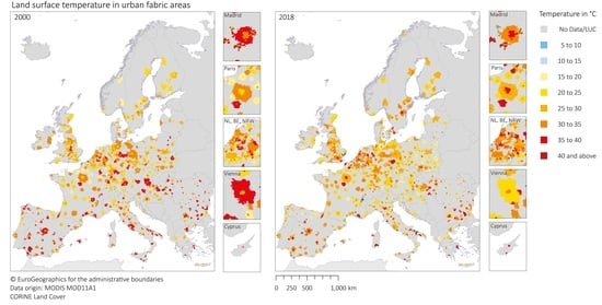
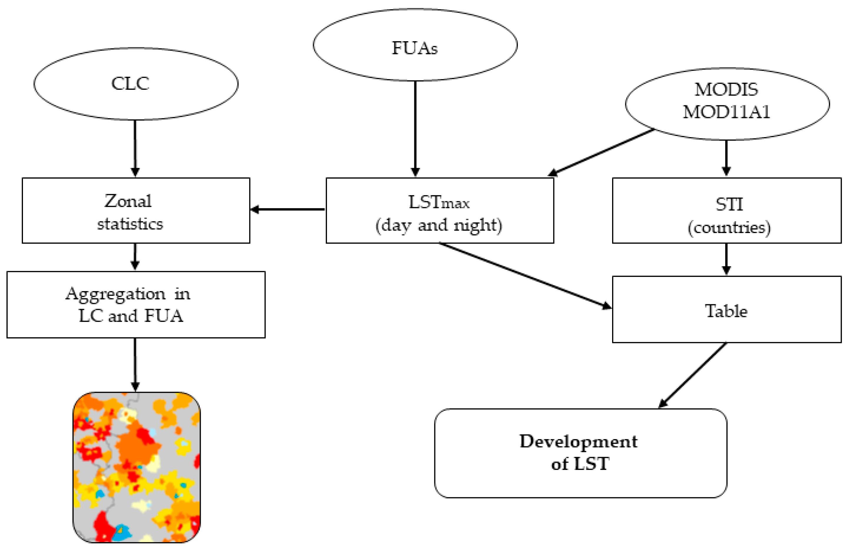
In the second step of how LSTs has developed in Europe in recent years, the maximum day LST of the period from June to October 2000 to 2020 were calculated. In order to obtain a uniform and consistent database of LST changes despite different climatic and weather conditions, the maximum LST of each year was used as the basis of the analysis. Data quality flags were not considered in the calculations because no LST product was generated in bad conditions, for example, due to cloud effects (flags 10 and 11). Impacts on the LST by thin cirrus or sub-pixel clouds were further reduced by retrieving the maximum values and would show deviations of ≤2 K in the worst case [52]. All preliminary calculations of the LST were performed with Google Earth Engine (GEE) [56]. The LST maxima were then aggregated by country, and a three-year moving average was calculated. In addition to a chronological sequence shown by the mean values for a city and surrounding area via zonal statistics as a table in ArcGIS, the LST were assigned to the areas of the Corine Land Cover (cf. Figure 2).
2.2.3. Land Use and Land Cover
In order to estimate the influence of land use and land cover on LST, Corine Land Cover data were used.
Land cover and land use are important indicators of environmental pressures and human activity. CORINE Land Cover (CLC) provides data on the European land area and how it changes. Since 1990, data have been considered and collected Europe-wide from a minimum mapping unit (MMU) of 25 ha for areas and 100 m for linear “phenomena”. Smaller areas are allocated to the next appropriate class according to a matrix, which is divided into 44 land cover and land use classes (cf. Table 2). With the second version in 2000, a temporal change in land use and land cover compared with 1990 was mapped for the first time, in addition to existing areas with an MMU of 5 ha. Further versions followed in 2006, 2012, and 2018. Although the data set is provided by EEA, it is mainly responsible for coordination, integration, and evaluation. Producing the national CLC databases is carried out by the Eionet network National Reference Centers Land Cover (NRC/LC) [57].
2.2.4. Calculation of CLC and LST
The CLC data were merged with the shapefiles of the FUAs using ‘Identity’ in ArcGIS. The area sizes were subsequently recalculated. Thus, each CLC polygon, the input feature, received the coding and attributes of the respective commuting zone or core, the identity features, and could be clearly assigned (cf. Figure 3).
In order to analyze the relationship between LST and urban use, the LST maxima of the MODIS product of each CLC polygon calculated in GEE were averaged using the zonal statistics function for the years 2000, 2006, 2012, and 2018. The output table includes the ID of each individual polygon, the land use code, the FUA code, and the average LST of each polygon.
For further analysis, the data were combined by means of frequency for core and commuting zone and then aggregated to different classes. Frequency is a tool in ArcGIS that statistically aggregates multi-polygons with the same properties. In this case, the mean values of the LSTs of each land use type in each FUA were aggregated. (cf. Table 2). The artificial surfaces and the 300 classes (in forest and nature) were further subdivided, e.g.,: 111 and 112 were combined to urban fabric, 121 to 124 were aggregated as industrial und infrastructure areas, 141 and 142 as urban green, and 211 to 244 grouped together as agriculture. The end product is a table that contains the average LSTs of each land use/ cover for all FUA’s in Europe, divided into core and commuting zone.
3. Results
3.1. LST Change
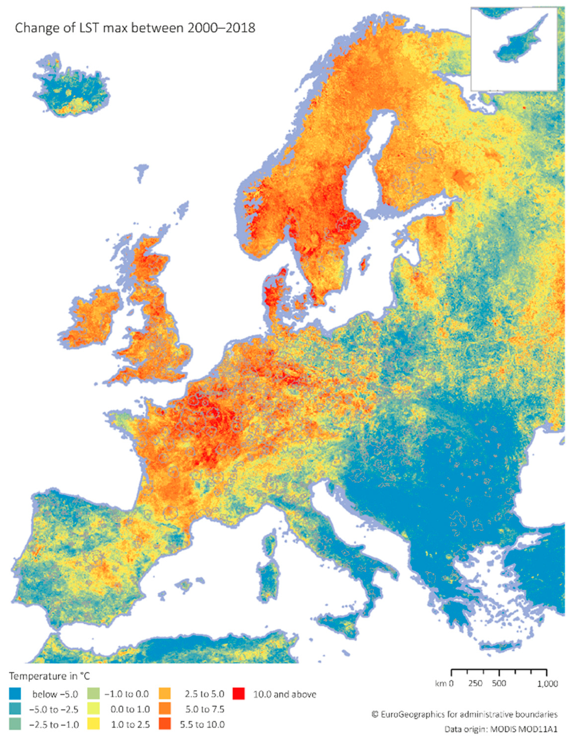
Figure 4 depicts the LST changes for the whole continent of Europe between 2000 and 2018, with a resolution of 1000 m. If one compares the LST differences between these years, it becomes clear that Europe, eastern Europe especially, had particularly higher LSTs in 2000. Higher LSTs compared to the previous period mainly occur in central Europe, Scandinavia, Finland, France and Great Britain (cf. Figure 4). A deeper investigation of the past LST development was carried out based on the selected FUAs and CLC classes.
3.1.1. LST in the First Two Weeks of August in Selected FUAs
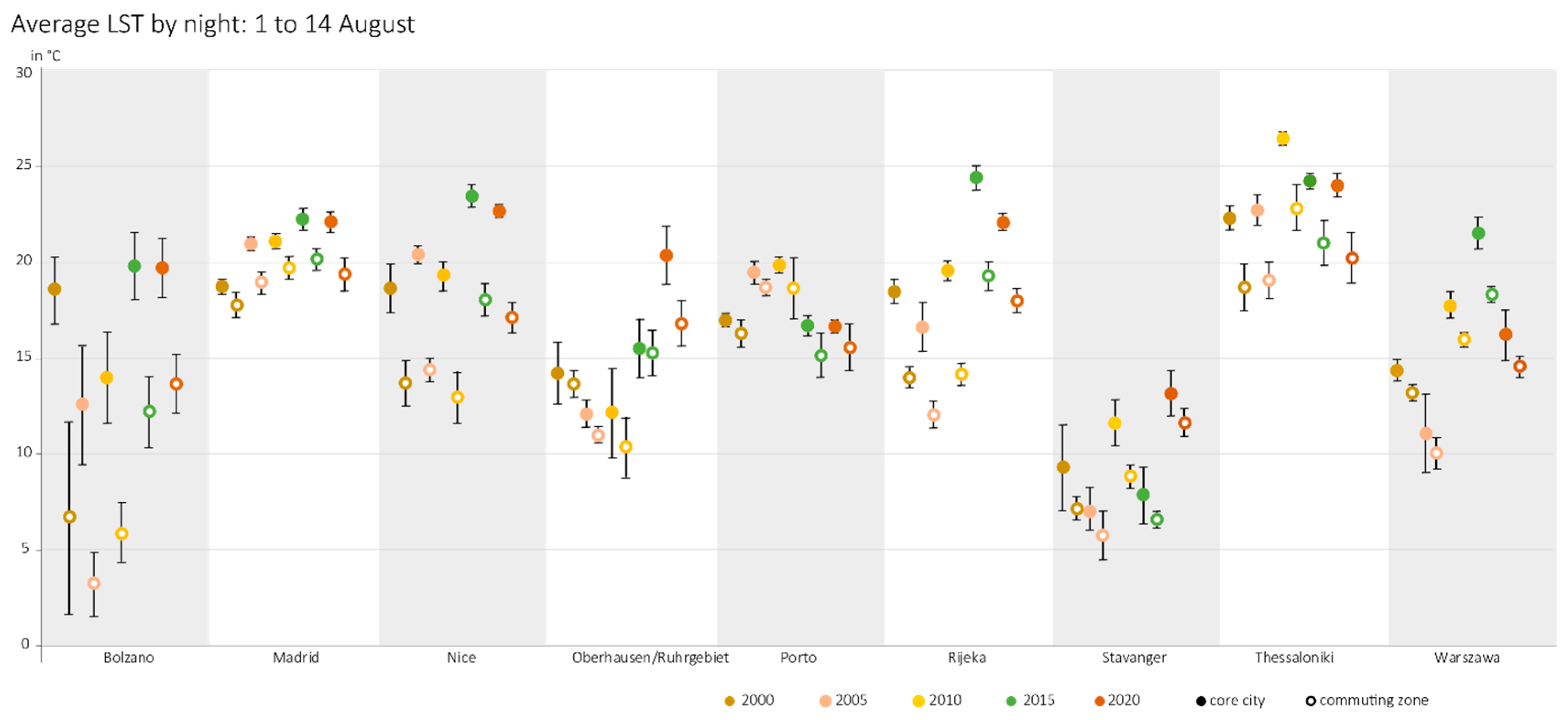
The different months of the above-average warm periods make it difficult to assess a development of SUHIs in recent years. As most heat anomalies occur in August (cf. Table 3), the LST of the first half of August in the whole period was calculated for better comparability (cf. Section 2.2.2).
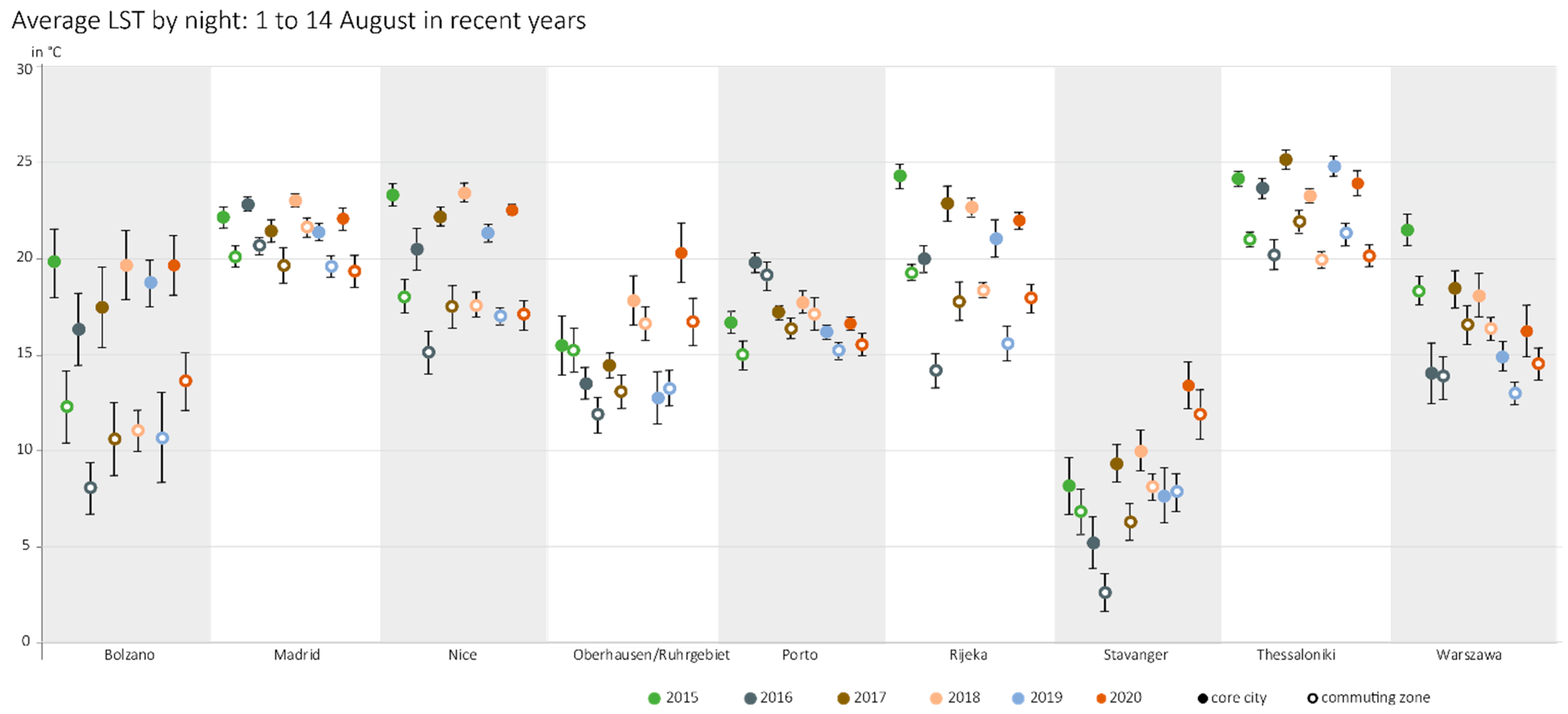
Comparing time series, FUAs with particularly high LST differences in the city and its surrounding area (taking the example of Bolzano, as well as additional cities) were then selected in order to cover the greatest possible geographical breadth of Europe.
Due to its location in the valley, the FUA of Bolzano, for example, shows particularly large LST differences between the core and the commuting zone, contrary to Porto where, due to its location on the Atlantic coast, this effect is less noticeable. In the city center of Madrid, night-time LST are also only marginally higher than in the densely built-up areas surrounding the city (cf. Figure 5). The examples of Oberhausen and Warsaw show that the difference between the city and its commuting zones increases with rising LST, i.e., less cooling effects at night (r = 0.68; p < 0.001) (cf. Figure 6). In contrast, the differences in cities in southern European countries, such as Madrid, Nice, Porto, Rijeka, and Thessaloniki, remain relatively constant, even at different LST. With the exception of Porto and Thessaloniki, the LST have shown a trend, with either 2015 or 2020 being the year with the highest values (cf. Figure 5).
The ratio of the urban-rural difference in the selected FUAs remains similar to previous periods. However, 2019 is a striking year, when the LST in the area surrounding the FUAs in the Ruhr Area and Stavanger were higher than in the centers. Whereas 2019 was the coldest year since 2015 in Oberhausen (Ruhr Area), in Stavanger, 2016 was significantly colder, but despite low LST, it shows a high disparity between the city and its commuting zones (cf. Figure 7).
The trend of perceiving the year over a long period of time has not been discernible in recent years. Instead of the “hottest” year, spatial patterns are emerging on the basis of which one tends to classify the regions according to climate zones. While it was particularly hot in 2015 in the FUAs of Rijeka and Warsaw, which are located more in the east of Europe, the hottest year of the two northernmost FUAs of the Ruhr Area and Stavanger was 2020. In Madrid and Nice it was 2018; the same as in Bolzano for three years (2015, 2018, and 2020 had equal values). The highest LST in Porto occurred in 2016, and in Thessaloniki it was in 2017; in 2019 none of the selected FUAs showed the highest LST in recent years (cf. Figure 7).
3.1.2. Development of LST Maxima from 2000 to 2020
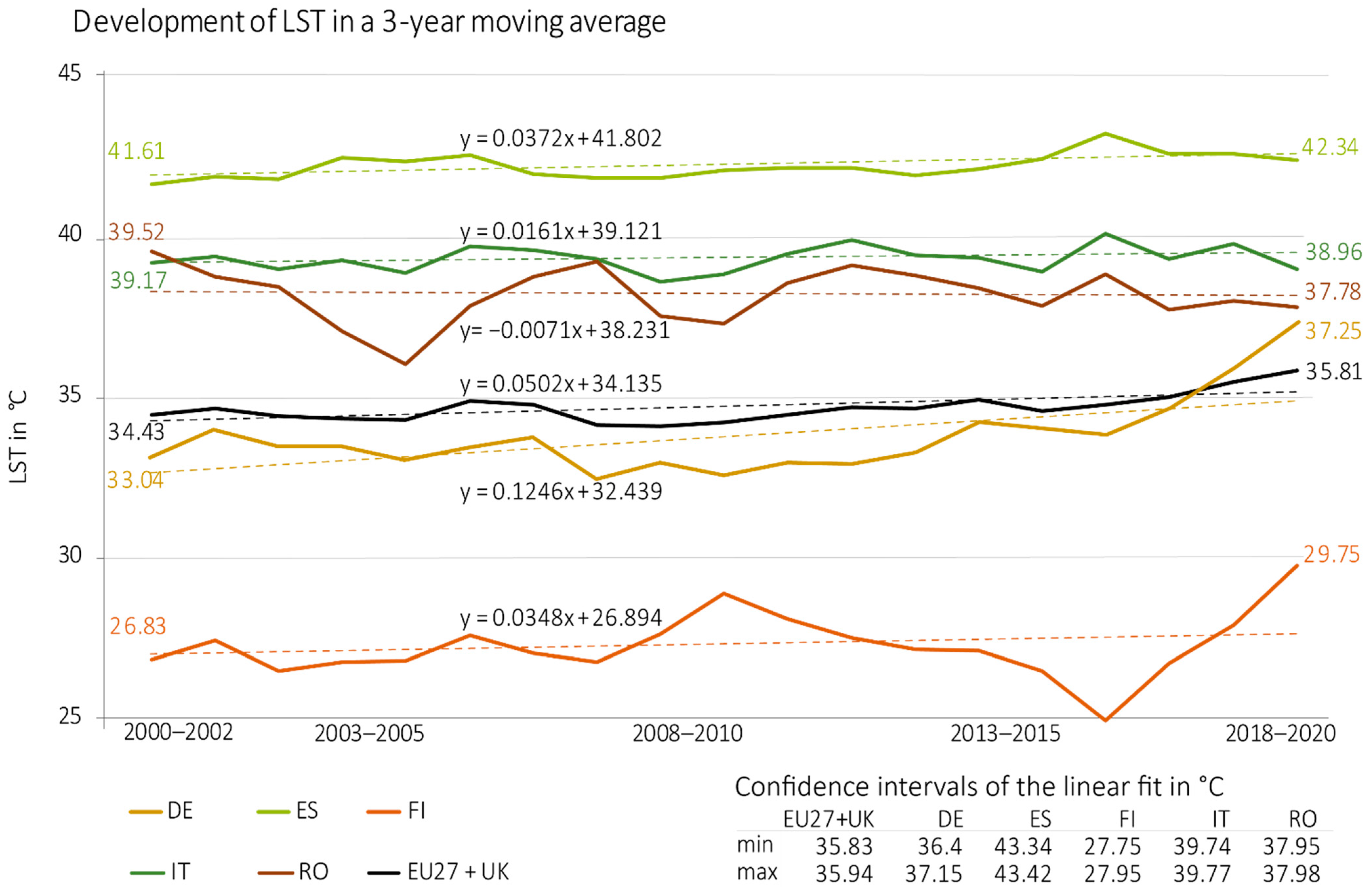
Differences in LST development can not only be seen in different FUAs but also in countries. Considering the fact that the LST maxima of all FUAs in Europe at the three-year moving window average from 2018 to 2020 were 35.81 °C, temperatures were about 1.4 °C higher than 20 years before; the LST in Romania and Italy is even below the LST at the beginning of the millennium, whereas in Italy the trend (y = 0.0161x) is still slightly increasing—in contrast to Romania (y = −0.0071x). In Spain, LST has risen but has stayed below the European average, while in Germany and Finland the increase is much higher, at a rate of 4 °C and almost 3 °C, respectively (cf. Figure 8).
3.2. LST of Different Land Use/Land Cover Types
However, for further analysis of the differences between the city and the surrounding area, not only the geographical location of the FUAs must be taken into account, but also their structure. This is obvious when looking at the LST of the built-up areas (CLC 110, 120, and 130) of the total European land area. The example of the maximum LST in 2018 shows quite clearly that they rise with the increasing density of built-up areas (cf. Figure 9).
LST differences in the individual land use classes in FUAs are therefore considered and explained in detail. For this purpose, the LST for the years 2000 and 2018 are considered in the land use classes summarized in: urban fabric, industrial and infrastructure areas, as well as green urban and agricultural areas (cf. Section 2.2.3 and Section 2.2.4).
If one compares the LST maps of built-up, urban green, and agricultural areas in 2000 (cf. Figure 10 and Figure 11) it turns out that the LSTs of more use-intensive areas, such as industrial and commercial areas, as well as those of the infrastructure (summarized below as industrial areas) and urban fabric, have clearly higher LSTs than the other two groups of uses, with the LSTs of urban green areas being clearly lower than those of agricultural areas.
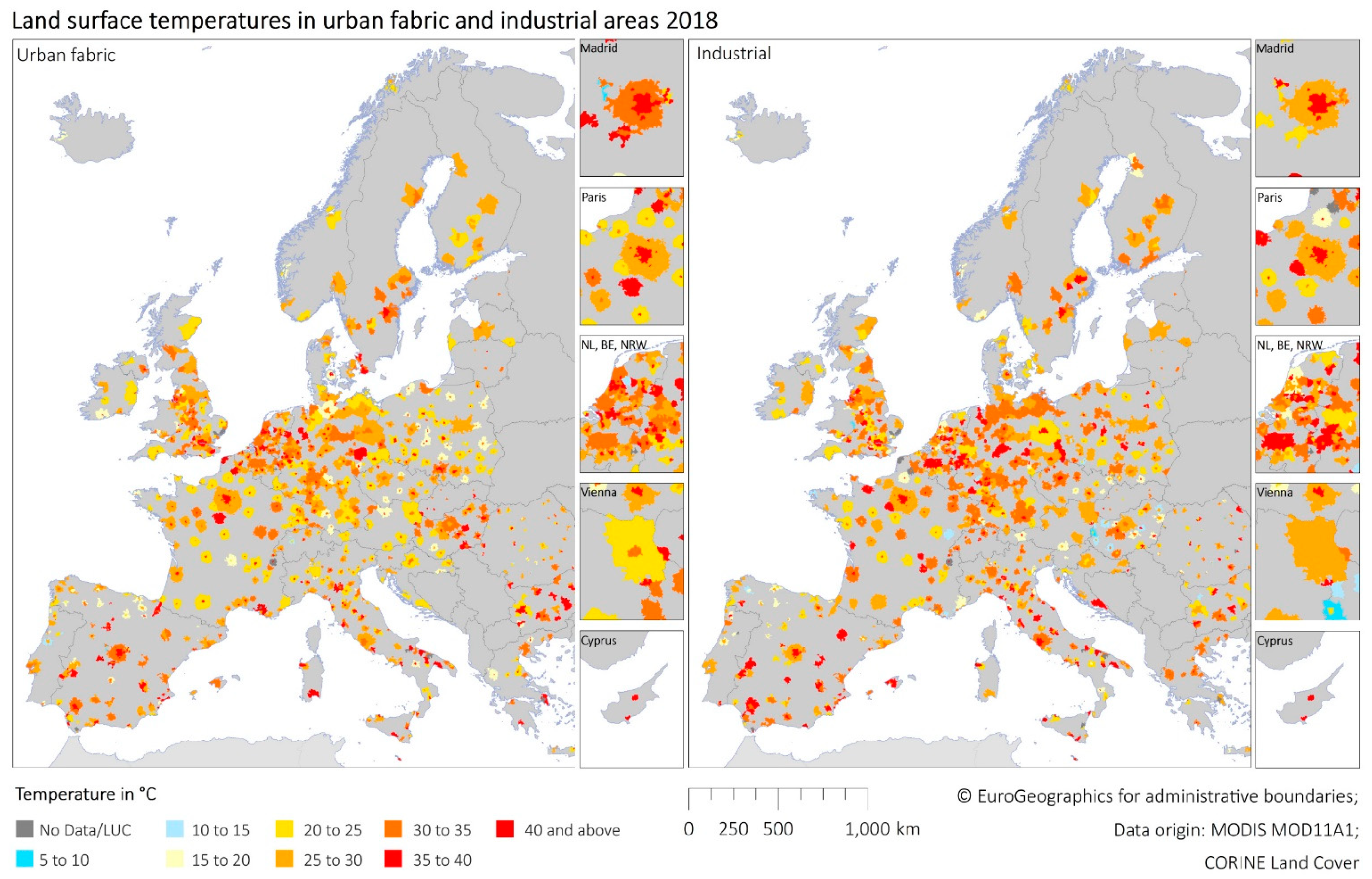
While the LSTs in the cores are highest in urban fabric areas, with an average of 26.13 °C, the LST in the surrounding areas are the highest in areas of industrial use, with an average of 28.63 °C, even if only slightly different (28.57 °C in urban fabric). A particular note in the Figures as well as in the average LST is that the LSTs within the cores are lower than those in the commuting zones (see Figure 10). This effect is particularly obvious in infrastructure areas, where the LST in the commuting zones is, on average, about 4 °C higher. In urban fabric areas, the effect can mainly be observed in larger cities and agglomerations.
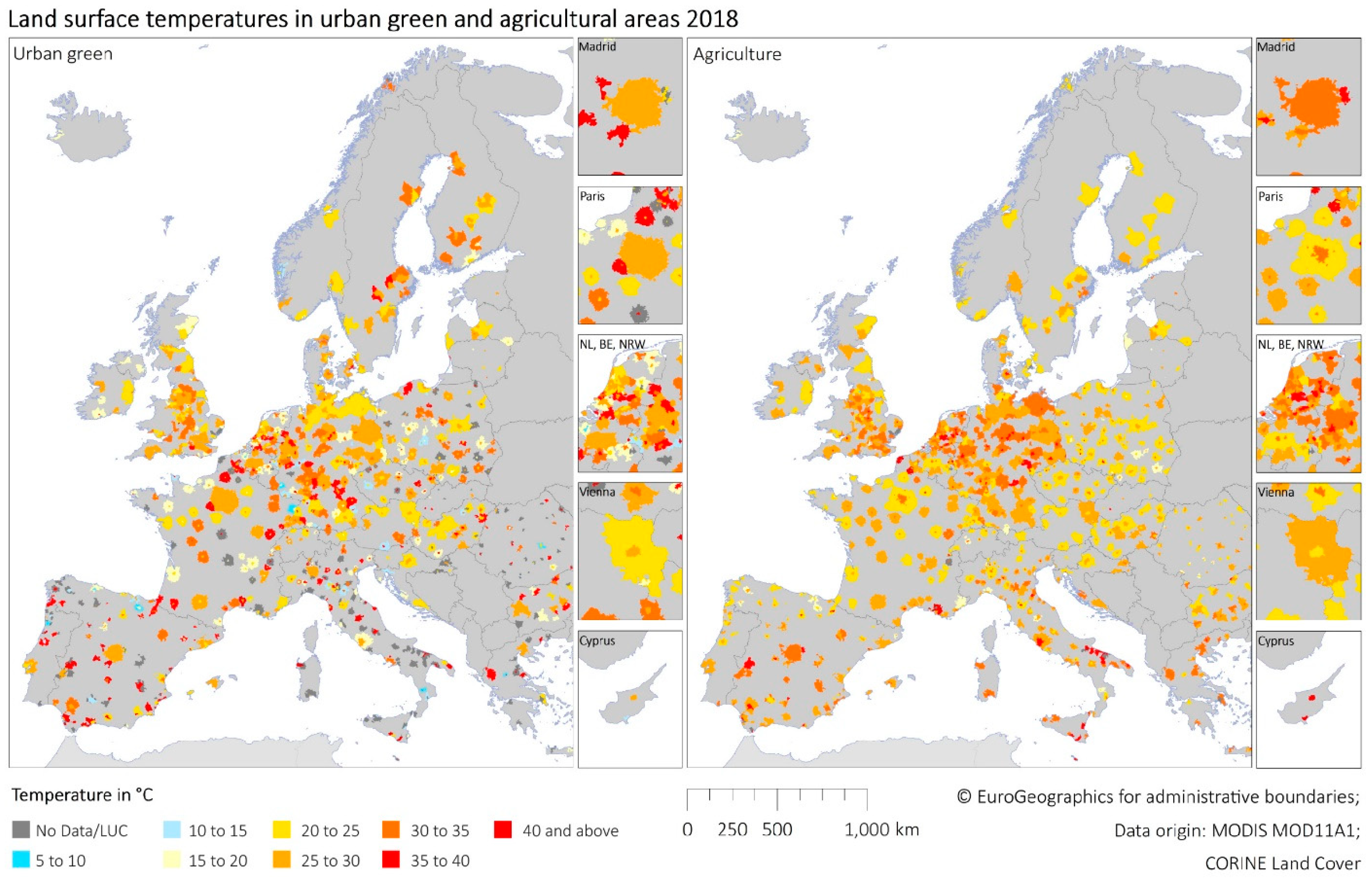
The LSTs of green urban areas are significantly lower than those of the more use-intensive areas, both in the city and in the surrounding countryside. In addition, the differences between core and commuting zone are larger. LSTs in green urban areas are about 6 °C below of those of the surrounding areas, at 18.62 °C in the cities. The significantly lower LSTs of urban green spaces suggest that the same applies for other vegetated areas such as agriculture. In the surrounding areas, LSTs in agricultural areas, at a rate of 28.39 °C, are similarly high as those in urban fabric and infrastructure areas, although the LSTs of agricultural areas in the cores, at an average of 24.19 °C, are comparable to those in urban areas (cf. Figure 11).
In 2018, the LSTs of urban fabric and infrastructure areas are again significantly higher than those of green urban areas. Within the cores, the areas of urban use are those with the highest LSTs (32.63 °C). Despite some relatively cooler commuting zones in Hungary and France, the highest LSTs can also be found in the infrastructure areas, with 27.76 °C, higher than the urban fabric areas, with an LST of 26.57 °C. The “reversal” of the differences between the city and its commuting zone is also clearly visible in the Figures (cf. Figure 12); the centers here now stand out very clearly from the surrounding areas, in the same way that the higher LSTs compared to 2000 are also visible.
The LSTs of the green urban and agricultural areas are 24.29 °C and 29.40 °C, respectively, with a similar difference to 2018—again below the LSTs in the urban areas. The LSTs of the green urban areas are now higher in the cores than in the surrounding areas and show the second-highest difference after the urban fabric areas with just under 4 °C. As in 2000, the LSTs of agricultural land show a more homogeneous picture, with recognizable spatial structures, and are the highest after those of urban fabric and urban infrastructure areas. As the average values suggest, the core LST of 29.40 °C is almost higher than those of the surrounding areas, with an average of 26.27 °C. Exceptions are again rather less extensive FUAs. The only larger FUA, where LST of agricultural land in 2018 is higher in the surrounding area, is Vienna. In Eastern Europe, LSTs are almost identical in all FUAs, with 20–25 °C in the surrounding areas and 25–30 °C and 30–35 °C in urban fabric and urban infrastructure areas, respectively. Spatial clusters with similar LSTs are also emerging in France and on the Iberian Peninsula. The LSTs of agricultural land in densely populated areas of the Benelux countries, Germany, and Great Britain are also strikingly high and comparable to the LSTs in southern Europe (cf. Figure 13).
The phenomenon of the warmer surrounding area in 2000 is illustrated for all types of use in Figure 14. The greatest LST differences to the city are found in forest areas and areas of terrestrial nature. The LSTs of forest areas, as well as urban fabric, infrastructure, and agriculture areas in the commuting zones were already below those of cities in 2006. In the case of non-urban areas, wetlands, and waterbodies, the LST will remain above this level throughout the entire period, but the difference gets smaller and smaller. The LSTs of green urban areas and terrestrial nature are still lower in 2006 in the cores than in the commuting zones, albeit a decreasing difference compared to 2000. In 2012 and 2018, however, the ratio is expected to reverse.
LSTs in the various forms of land use are highest over the entire period in the urban fabric areas, followed by infrastructure and agricultural areas. With the exception of 2000, the lowest LSTs can be found in the wetlands areas. The LSTs of areas with vegetation are lower in the green urban areas than in the forest areas, again with the exception of 2000.
4. Discussion
If one looks at the LST change in the FUAs, the trend of an increase in temperature in recent years is quite clear; the EEA also states that observational data show a continuous increase in heat extremes over land [58]. Looking at the LST maxima of all FUAs in Europe, considering the three-year average in 2018–2020 of 35.81 °C, temperatures are 1.4 °C higher than 20 years before, while the average annual temperature of European land areas in the last decade (2010–2019) was about 1.7 °C to 1.9 °C higher than in the pre-industrial period, turning this decade into the warmest ever in Europe [59].
The results for the first half of August also show that the LSTs have risen overall and the last few years have been warmer. The urban-rural difference is higher at high LSTs in regions of lower LSTs, such as Oberhausen, Stavanger, Warsaw, and Bolzano, while it remains relatively constant in Madrid, Nice, Porto, Rijeka, and Thessaloniki, regardless of the respective LST. The effect of stronger night-time SUHIs in cold-drier cities than in humid-warmer cities has also been described in other studies [60].
The development of the difference between the city and the surrounding area, with higher LSTs in the surrounding area compared to the city in 2000 and vice versa in 2018, is only partially visible in comparative studies. Analyses that examined global changes in SUHIs in connection to climate change tend to show different trends with higher temperature increases in rural areas compared to cities, and the other way round [61,62]. Local studies especially demonstrate a development comparable to this study [63].
The growth of cities in the decades to come is expected to increase the SUHI effect and further intensify the heat stress in cities in addition to the temperature increase due to climate change [26,64]. Zhou et al. [27] argue that land cover and its changes are undeniably among the most important factors influencing UHI. For example, the presence of buildings and sealed surfaces leads to an increase in LST, whereas urban green areas have a cooling effect [65,66]. The analyses in Section 3.2 show a strong correlation between higher LSTs and built-up areas and conversely between lower LSTs and forests and urban green. Comparable results are explained by Bechtel et al. [14] for the relationship between LST and the local climate zones (LCZ) of cities. In particular, compact LCZ types and commercial/industrial LCZ types have stronger SUHI intensities than open ones. In addition, all cities show positive SUHI values for the built-up classes. The effect of a higher proportion of built-up areas and higher LSTs is also clearly evident in the commuting zones, while this correlation also exists in the cores, but less clearly, although the composition of urban structures is often considered more important than its arrangement [67,68].
According to Adachi et al. [69], the highest LSTs are found in the densest areas of a city. These temperature fluctuations can also be assumed in the European analysis, as the LST of the individual land use classes of an FUA showed partly significant differences (cf. Section 3.2). Research also shows that land cover and land use may not only lead to urban-rural temperature gradients, but also to inner-city temperature differences [27,37]. Urban differences typically manifest themselves in a spatial cluster of hot and cold spots, which can sometimes even be larger than the temperature gradient between urban and rural areas [27].
However, as industrial areas, for example, are often among the hottest places in urban environments due to high heat emissions, land use must be included in the analyses in addition to land cover [31]. It can particularly be seen that LSTs in industrial areas, especially in the surrounding areas, are comparable to or higher than those in urban fabric areas (cf. Section 3.2.; [32]).
High LSTs in agricultural land and lower differences between urban and rural areas, as is evident for Europe as a whole, can be explained by increased soil dryness, which leads to a reduction in the rural evaporation rate [61].
The analyses of developments of various kind in the present study are too brief and require a more in-depth analysis. The simple comparison of years in particular does not show the actual LST change in a city, but compares two snapshots, which can be used to produce an initial overview and extract individual trends but are not suitable for a deeper analysis. By using the maximum LST of each year, an attempt was made to create a uniform and consistent data basis providing a sound basis for the analysis of the LST development despite different weather conditions. High differences between core and commuting zone of different land uses (such as 2018 in and around Paris) may result from the poor resolution of the MODIS LST product. In particular, smaller sealed areas, for example, are distorted by adjacent water or natural areas because the mean value over all areas is lower here. Conversely, in the cores, the LST of a tile over urban green spaces can be increased by neighboring buildings. Other sources of uncertainty in comparing LSTs in different land uses/covers can also be identified in the CLC dataset. Identifying and mapping specific patterns in an urban context can be made difficult due to differences in classification between countries. While most datasets are classified through the use of high-resolution satellite imagery, there are others that are based on semi-automated processes using both in-situ data and satellite imagery, generalizations, and GIS integrations [57,70]. In addition to land use and land cover, elevation also affects LST, as can be seen very clearly in the example of Bolzano. However, these effects were not taken into account in this paper. Furthermore, it is to be taken into account that LST changes over the years can not only be influenced by urbanization or climate change; even climate oscillations such as NAO, ENSO, or climate variability can also have an impact on LST.
5. Conclusions
The evolution of LST in European cities in recent years shows a clear trend of rising LST. A higher incidence of urban centers is particularly noticeable in places with a high proportion of built-up areas. Therefore, a connection exists between higher LSTs within built-up areas as opposed to LSTs in urban green areas and forests. In 2018, the averaged LST in the cores in urban use areas was 32.63 °C, and in green urban areas it was 24.29 °C. Apart from that, agricultural areas sometimes show similarly high LSTs to built-up areas. Thus, the average LST in commuting zones in urban use areas was 28.57 °C, and in industrial areas it was 28.63 °C; agriculture had 28.39 °C in comparison. Urban density is a key factor in the spatial variability of SUHIs, and higher LSTs often occur in the densest parts of the city (cf. Figure 9), potentially exposing the inhabitants of these areas to high levels of heat stress. Nevertheless, many local studies have so far only examined one urban land use type rather than the variability of density within the city. In addition, urbanization has mainly been considered in terms of expansion; other urban planning instruments, such as re-densification, have been completely ignored. However, the first approach of the present study towards including the different land use classes of a city in the consideration is too limited and needs to be further elaborated in further studies by means of a more detailed analysis and, for example, comparisons of LST within the identified morphology. In future analyses, the possibility of downscaling to 100 m, as has already been done locally, would need to be considered to accommodate both resolutions.
Apart from that, the analysis of the different densities should be validated on a large scale or at least with further case studies for a more precise validation. The need for research in the field of re-densification and land use changes will continue to grow in importance in the future, as it is already part of almost all urban development plans, though, SUHI effects have so far mainly been studied in the context of suburbanization. Estimating the development of heat islands is absolutely unrealistic on the basis of a pure analysis of expansion; future studies should thus aim to include more realistic scenarios of urban growth, e.g., by applying government plans when designing scenarios. In addition, the separate considerations of climate change and urban growth should not be neglected, as this would lead to a stronger increase in temperature than considering either of the two factors alone. A better understanding of the processes by which climate change or urban growth increase or decrease the SUHI will help to identify particularly vulnerable urban areas. If either climate change or urban growth is excluded, the effects of the future urban LST would be underestimated.
Author Contributions
Conceptualization, A.H. and A.R., formal analysis, A.H.; writing—original draft preparation, A.H.; writing—review and editing, A.H. and A.R. All authors have read and agreed to the published version of the manuscript.
Funding
This research received no external funding.
Data Availability Statement
Not applicable.
Acknowledgments
We would like to thank Julia Dahm, André Mueller, and Beatrix Thul for proofreading and Google for providing free access to the Google Earth Engine.
Conflicts of Interest
The authors declare no conflict of interest.
References
- Ruppert, T.; Sparwasser, N.; Taubenböck, H. Temperatureffekte in der Stadt-Umland-Region München. In Fernerkundung im urbanen Raum—Erdbeobachtung Auf dem Weg zur Planungspraxis; Taubenböck, H., Dech, S., Eds.; Wissenschaftliche Buchgesellschaft: Darmstadt, Germany, 2010; pp. 62–65. [Google Scholar]
- Dikau, R.; Pohl, J. Hazards: Naturgefahren und Naturrisiken. In Geographie. Physische Geographie und Humangeographie; Gebhardt, H., Ed.; Spektrum Akademischer Verlag: Berlin/Heidelberg, Germany, 2011; pp. 1114–1169. [Google Scholar]
- Schmidt-Seiwert, V.; Duvernet, C.; Hellings, A.; Gauk, M.; Binot, R.; Kiel, L.; Thul, B. Atlas for the Territorial Agenda. Maps on European Territorial Development; Building and Community (BMI) Federal Ministry of the Interior and Urban Affairs and Spatial Development (BBSR) Federal Institute for Research on Building: Berlin, Germany, 2020. [Google Scholar]
- European Union. Urban Data Platform Plus. Territorial Trends. Total Population—Projections. Set of Indicators Produced by the LUISA Modelling Platform. Available online: https://urban.jrc.ec.europa.eu/#/en/trends?context=Default&territorialscope=EU28&level=FUA&indicator=POP_LUISA_PROJ (accessed on 23 March 2021).
- Naumann, G.; Russo, S.; Formetta, G.; Ibaretta, D.; Forzieri, G.; Girardello, M.; Feyen, L. Global Warming and Human Impacts of Heat and Cold Extremes in the EU; JRC PESETA IV Project—Task 11; Publications Office of the European Union: Luxembourg, 2020. [Google Scholar]
- Kemen, J.; Schäfer-Gemein, S.; Kistemann, T. Klimaanpassung und Hitzeaktionspläne. In Informationen zu Raumentwicklung; BBSR; Franz Steiner Verlag: Stuttgart, Germany, 2020; Volume 47, pp. 58–69. [Google Scholar]
- IPCC, Intergovernmental Panel on Climate Change. Climate Change 2001: Impacts, Adaption, Vulnerability; McCarths, J.J., Ed.; Contribution of Working Group II to the Third Assessment Report of the Intergovernmental Panel on Climate Change; Cambridge University Press: Cambridge, UK, 2001. [Google Scholar]
- Parlow, E. Besonderheiten des Stadtklimas. In Geographie. Physische Geographie und Humangeographie; Gebhardt, H., Ed.; Spektrum Akademischer Verlag: Heidelberg, Germany, 2011; pp. 287–294. [Google Scholar]
- Arnfield, A.J. Two Decades of Urban Climate Research: A Review of Turbulence, Exchanges of Energy and Water, and the Urban Heat Island. Int. J. Climatol. 2003, 23, 1–26. [Google Scholar] [CrossRef]
- Zhou, X.; Chen, H. Impact of urbanization-related land use land cover changes and urban morphology changes on the urban heat island phenomenon. Sci. Total Environ. 2018, 635, 1467–1476. [Google Scholar] [CrossRef]
- Li, X.; Zhou, Y.; Asrar, G.R.; Imhoff, M.; Li, X. The surface urban heat island response to urban expansion: A panel analysis for the conterminous United States. Sci. Total Environ. 2017, 605–606, 426–435. [Google Scholar] [CrossRef]
- Bechtel, B.; Zakšek, K.; Hoshyaripour, G. Downscaling Land Surface Temperature in Urban Area: A Case Study for Hamburg, Germany. Remote Sens. 2012, 4, 3184–3200. [Google Scholar] [CrossRef] [Green Version]
- Sismanidis, P.; Keramitsoglou, I.; Kiranoudis, C.T.; Bechtel, B. Assessing the Capability of a Downscaled Urban Land Surface Temperature Time Series to Reproduce the Spatiotemporal Features of the Original Data. Remote Sens. 2016, 8, 274. [Google Scholar] [CrossRef] [Green Version]
- Bechtel, B.; Demuzere, M.; Mills, G.; Zhan, W.; Sismanidis, P.; Small, C.; Voogt, J. SUHI analysis using Local Climate Zones—A comparison of 50 cities. Urban Clim. 2019, 28, 100451. [Google Scholar] [CrossRef]
- Oke, T.R.; Mills, G.; Christen, A.; Voogt, J.A. Urban Climates. In Urban Heat Island; Cambridge University Press: Cambridge, UK, 2017; pp. 197–237. [Google Scholar] [CrossRef] [Green Version]
- Martilli, A.; Roth, M.; Chow, W.; Demuzere, M.; Lipson, M.; Krayenhoff, E.S.; Sailor, D.; Nazarian, N.; Voogt, J.; Wouters, H.; et al. Summer Average Urban-Rural Surface Temperature Differences Do Not Indicate the Need for Urban Heat Reduction. Available online: osf.io/8gnbf (accessed on 12 February 2021).
- Mitraka, Z.; Chrysoulakis, N.; Doxani, G.; Del Frate, F.; Berger, M. Urban Surface Temperature Time Series Estimation at the Local Scale by Spatial-Spectral Unmixing of Satellite Observations. Remote Sens. 2015, 7, 4139–4156. [Google Scholar] [CrossRef] [Green Version]
- Sismanidis, P.; Keramitsoglou, I.; Kiranoudis, C.T. A satellite-based system for continuous monitoring of Surface Urban Heat Islands. Urban Clim. 2015, 14, 141–153. [Google Scholar] [CrossRef]
- Kraus, H. Die Atmosphäre der Erde. Eine Einführung in die Meteorologie, 3rd ed.; Springer: Berlin/Heidelberg, Germany, 2004. [Google Scholar]
- Coackley, J.A. Reflectance and Albedo, Surface. In Encyclopedia of the Atmosphere; Academic Press: Cambridge, MA, USA, 2003; pp. 1914–1923. [Google Scholar]
- Kuchling, H. Taschenbuch der Physik; Carl Hanser Verlag: Munich, Germany, 2011. [Google Scholar]
- Monteith, J.L. Evaporation and surface temperature. Q. J. R. Meteorol. Soc. 1981, 107, 1–27. [Google Scholar] [CrossRef]
- NASA. Land Surface Temperature. Available online: https://earthobservatory.nasa.gov/global-maps/MOD_LSTD_M (accessed on 1 April 2021).
- Keramitsoglou, I.; Kiranoudis, C.T.; Ceriola, G.; Weng, Q.; Rajasekar, U. Identification and analysis of urban surface temperature patterns in Greater Athens, Greece, using MODIS imagery. Remote Sens. Environ. 2011, 115, 3080–3090. [Google Scholar] [CrossRef]
- Voogt, J.A.; Oke, T.R. Thermal remote sensing of urban climates. Remote Sens. Environ. 2003, 86, 370–384. [Google Scholar] [CrossRef]
- Zhu, Z.; Zhou, Y.; Seto, K.C.; Stokes, E.C.; Deng, C.; Pickett, S.T.A.; Taubenböck, H. Understanding an Urbanizing Planet: Strategic Directions for Remote Sensing. Remote Sens. Environ. 2019, 228, 164–182. [Google Scholar] [CrossRef]
- Zhou, D.; Xiao, J.; Bonafoni, S.; Berger, C.; Deilami, K.; Zhou, Y.; Frolking, S.; Yao, R.; Qiao, Z.; Sobrino, J.A. Satellite Remote Sensing of Surface Urban Heat Islands: Progress, Challenges, and Perspectives. Remote Sens. 2019, 11, 48. [Google Scholar] [CrossRef] [Green Version]
- Yue, W.; Liu, Y.; Fan, P.; Ye, X.; Wu, C. Assessing spatial pattern of urban thermal environment in Shanghai, China. Stoch. Environ. Res. Risk Assess. 2012, 26, 899–911. [Google Scholar] [CrossRef]
- Pan, J. Analysis of human factors on urban heat island and simulation of urban thermal environment in Lanzhou city, China. J. Appl. Remote Sens. 2015, 9, 1. [Google Scholar] [CrossRef]
- Hart, M.A.; Sailor, D.J. Quantifying the influence of land-use and surface characteristics on spatial variability in the urban heat island. Theor. Appl. Climatol. 2009, 95, 397–406. [Google Scholar] [CrossRef]
- Li, J.; Song, C.; Cao, L.; Zhu, F.; Meng, X.; Wu, J. Impacts of landscape structure on surface urban heat islands: A case study of Shanghai, China. Remote Sens. Environ. 2011, 115, 3249–3263. [Google Scholar] [CrossRef]
- Roth, M.; Oke, T.R.; Emery, W.J. Satellite-derived urban heat islands from three coastal cities and the utilization of such data in urban climatology. Int. J. Remote Sens. 1989, 10, 1699–1720. [Google Scholar] [CrossRef]
- Du, P.; Chen, J.; Bai, X.; Han, W. Understanding the seasonal variations of land surface temperature in Nanjing urban area based on local climate zone. Urban Clim. 2020, 33, 100657. [Google Scholar] [CrossRef]
- Stewart, I.D.; Oke, T.R. Local Climate Zones for Urban Temperature Studies. Bull. Am. Meteorol. Soc. 2012, 93, 1879–1900. [Google Scholar] [CrossRef]
- Reicher, C. Staedtebauliches Entwerfen; Springer: Wiesbaden, Germany, 2017. [Google Scholar]
- Dose, M. Eine Analyse des Ist-Zustandes sowie planungs-bzw. umweltrechtlicher Instrumente zur Optimierung der Freiraumqualitaeten. In Soziale und Oekologische Freiraumqualitaeten Suburbaner Gewerbegebiete; Technical University of Berlin: Berlin, Germany, 2004. [Google Scholar]
- Fenner, D.; Meier, F.; Bechtel, B.; Otto, M.; Scherer, D. Intra and inter ‘local climate zone’ variability of air temperature as observed by crowdsourced citizen weather stations in Berlin, Germany. Meteorol. Z. 2017, 26, 525–547. [Google Scholar] [CrossRef]
- Zhou, B.; Rybski, D.; Kropp, J.P. On the statistics of urban heat island intensity. Geophys. Res. Lett. 2013, 40, 5486–5491. [Google Scholar] [CrossRef]
- Bechtel, B. (Ed.) Earsel keynote speach: Urban Climate & Urban Green. Urban environmental change from space. In EARSeL Joint Workshop 2021. EO for Sustainable Cities and Communities; The Centre for Research and Technology: Liège, Belgium, 2021. [Google Scholar]
- Schwarz, N.; Lautenbach, S.; Seppelt, R. Exploring indicators for quantifying surface urban heat islands of European cities with MODIS land surface temperatures. Remote Sens. Environ. 2011, 115, 3175–3186. [Google Scholar] [CrossRef]
- Schwarz, N.; Manceur, A. Analyzing the Influence of Urban Forms on Surface Urban Heat Islands in Europe. J. Urban Plan. Dev. 2014, 141. [Google Scholar] [CrossRef]
- Zhou, B.; Rybski, D.; Kropp, J.P. The role of city size and urban form in the surface urban heat island. Sci. Rep. 2017, 4791, 1–9. [Google Scholar] [CrossRef] [PubMed]
- Schneider, A.; Friedl, M.A.; Potere, D. Mapping global urban areas using MODIS 500-m data: New methods and datasets based on ‘urban ecoregions’. Remote Sens. Environ. 2010, 114, 1733–1746. [Google Scholar] [CrossRef]
- Zhao, S.; Zhou, D.; Liu, S. Data concurrency is required for estimating urban heat island intensity. Environ. Pollut. 2016, 208, 118–124. [Google Scholar] [CrossRef]
- Cui, Y.; Xu, X.; Dong, J.; Qin, Y. Influence of Urbanization Factors on Surface Urban Heat Island Intensity: A comparison of Countries at Different Developmental Phases. Sustainability 2016, 8, 706. [Google Scholar] [CrossRef] [Green Version]
- European Union. Living in the EU. Size and Population. Available online: https://europa.eu/european-union/about-eu/figures/living_en (accessed on 14 September 2020).
- Schmidt-Seiwert, V.; Hellings, A. Nachhaltige Landnutzungsveränderungen und Urbanisierung in Europa? Inf. Forsch. BBSR 2020, 4, 2. [Google Scholar]
- Eurostat. Urban Audit 2020—Area Management—Dataset. Available online: https://ec.europa.eu/eurostat/web/gisco/geodata/reference-data/administrative-units-statistical-units/urban-audit (accessed on 21 January 2021).
- Dijkstra, L.; Poelman, H.; Veneri, P. The EU-OECD Definition of a Functional Urban Area; OECD Regional Working Papers; OECD: Paris, France, 2019; Volume 11/2019, pp. 1–18. [Google Scholar] [CrossRef]
- Snyder, W.C.; Wan, Z.; Zhang, Y.; Feng, Y.-Z. Classification-based emissivity for land surface temperature measurement from space. Int. J. Remote Sens. 1998, 19, 2753–2774. [Google Scholar] [CrossRef]
- Wan, Z. MODIS Land-Surface Temperature Algorithm Theoretical Basis Document (LST ATBD); Version 3.3; University of California: Santa Barbara, CA, USA, 1999. [Google Scholar]
- Wang, K.; Liu, J.; Wan, Z.; Wang, P.; Sparrow, M.; Haginoya, S. Preliminary accuracy assessment of MODIS land surface temperature products at a semi-desert site. SPIE Int. Soc. Optical Eng. 2005, 5832, 452–461. [Google Scholar]
- Mao, K.; Qin, Z.; Shi, J.; Gong, P. A practical spilt-window algorithm for retrieving land-surface temperature from MODIS data. Int. J. Remote Sens. 2005, 26, 3181–3204. [Google Scholar] [CrossRef]
- Deutscher Wetterdienst, DWD. Standardized Temperature Index (STI). Available online: https://www.dwd.de/DE/fachnutzer/landwirtschaft/dokumentationen/agrowetter/sti.pdf?__blob=publicationFile&v=3 (accessed on 26 July 2020).
- Fasel, M. Calculation of the Standardized Temperature Index. Package ‘STI’. Available online: https://cran.r-project.org/web/packages/STI/STI.pdf (accessed on 28 July 2020).
- Gorelick, N.; Hancher, M.; Dixon, M.; Ilyushchenko, S.; Thau, D.; Moore, R. Google Earth Engine: Planetary-scale geospatial analysis for everyone. Remote Sens. Environ. 2017, 202, 18–27. [Google Scholar] [CrossRef]
- Copernicus Programme. CORINE Land Cover. Available online: https://land.copernicus.eu/pan-european/corine-land-cover (accessed on 26 August 2020).
- EEA. European Environment Agency. Global and European Temperature. Available online: https://www.eea.europa.eu/data-and-maps/indicators/global-and-european-temperature-9/assessment (accessed on 21 August 2020).
- EEA. European Environment Agency. Indicator Assessment. Global and European temperatures. Available online: https://www.eea.europa.eu/data-and-maps/indicators/global-and-european-temperature-10/assessment (accessed on 1 October 2020).
- Wang, J.; Huang, B.; Fu, D.; Atkinson, P.M. Spatiotemporal Variation in Surface Urban Heat Island Intensity and Associated Determinants across Major Chinese Cities. Remote Sens. 2015, 7, 3670–3689. [Google Scholar] [CrossRef] [Green Version]
- Oleson, K. Contrasts between Urban and Rural Climate in CCSM4 CMIP5 Climate Change Scenarios. J. Clim. 2012, 25, 1390–1412. [Google Scholar] [CrossRef]
- Lau, K.K.-L.; Lindberg, F.; Rayner, D.; Thorsson, S. The effect of urban geometry on mean radiant temperature under future climate change: A study of three European cities. Int. J. Biometeorol. 2014, 59, 799–814. [Google Scholar] [CrossRef] [PubMed]
- McCarthy, M.P.; Best, M.J.; Betts, R.A. Climate change in cities due to global warming and urban effects. Geophys. Res. Lett. 2010, 37, 1–5. [Google Scholar] [CrossRef] [Green Version]
- IPCC, Intergovernmental Panel on Climate Change. Climate Change 2014. Impacts, Adaption, and Vulnerability. Part; A. Global and Sectoral Aspects; Field, C.B., Ed.; Cambridge University Press: New York, NY, USA, 2014. [Google Scholar]
- Buyantuyev, A.; Wu, J. Urban heat islands and landscape heterogeneity: Linking spatiotemporal variations in surface temperatures to land-cover and socioeconomic patterns. Landsc. Ecol. 2010, 25, 17–33. [Google Scholar] [CrossRef]
- Bowler, D.E.; Buyung-Ali, L.; Knight, T.M.; Pullin, A. Urban greening to cool towns and cities: A systematic review of the empirical evidence. Landsc. Urban Plan. 2010, 97, 147–155. [Google Scholar] [CrossRef]
- Peng, J.; Xie, P.; Liu, Y.; Ma, J. Urban thermal environment dynamics and associated landscape pattern factors: A case study in the Beijing metropolitan region. Remote. Sens. Environ. 2016, 173, 145–155. [Google Scholar] [CrossRef]
- Zhou, W.; Huang, G.; Cadenasso, M.L. Does spatial configuration matter? Understanding the effects of land cover pattern on land surface temperature in urban landscapes. Landsc. Urban Plan. 2011, 102, 54–63. [Google Scholar] [CrossRef]
- Adachi, S.; Kimura, F.; Kusaka, H.; Duda, M.G.; Yamagata, Y.; Seya, H.; Nakamichi, K.; Aoyagi, T. Moderation of Summertime Heat Island Phenomena via Modification of the Urban Form in the Tokyo Metropolitan Area. J. Appl. Meteorol. Clim. 2014, 53, 1886–1900. [Google Scholar] [CrossRef]
- Ehlert, I.; Schweitzer, C. (Eds.) Copernicus für das Umweltmonitoring. Eine Einführung; Copernicus: Hamburg, Germany, 2018. [Google Scholar]
Figure 1.
Location of selected FUAs.

Figure 2.
Methodology. With CLC as Corine Land Cover, LC as land cover, FUA as functional urban areas, LST as Land Surface LST, and STI as Standardized Temperature Index.
Figure 2.
Methodology. With CLC as Corine Land Cover, LC as land cover, FUA as functional urban areas, LST as Land Surface LST, and STI as Standardized Temperature Index.

Figure 3.
Identity tool in ArcGIS.

Figure 4.
Change of maximum LST 2000–2018. Calculated from MODIS MOD11A1.

Figure 5.
Average LST by night: 1 to 14 August in selected FUAs and years.

Figure 6.
LST difference in Oberhausen and Warsaw 2000–2020.

Figure 7.
Average LST by night: 1 to 14 August in selected FUAs in recent years.

Figure 8.
LST change trends at a three-year moving window average during the period from 2000 to 2020. In Germany (DE), Spain (ES), Finland (FI), Italy (IT), and Romania (RO) compared to the member states of the European Union and United Kingdom (EU27 + UK).
Figure 8.
LST change trends at a three-year moving window average during the period from 2000 to 2020. In Germany (DE), Spain (ES), Finland (FI), Italy (IT), and Romania (RO) compared to the member states of the European Union and United Kingdom (EU27 + UK).

Figure 9.
LST in built-up areas.

Figure 10.
LST of urban fabric and industrial areas, 2000.

Figure 11.
LST of urban green and agricultural areas, 2000.

Figure 12.
LST of urban fabric and industrial areas, 2018.

Figure 13.
LST of urban green and agricultural areas, 2018.

Figure 14.
LST of different land covers in core and commuting zone of different years.


Table 1.
STI values and conditions [54].
Table 1.
STI values and conditions [54].
| Conditions | STI |
|---|---|
| Extremely hot | ≥2.00 |
| Very hot | ≥1.50 and <2.00 |
| Moderately hot | ≥1.00 and <1.50 |
| Near normal | <1.00 and >−1.00 |
| Moderately cold | ≤−1.00 and >−1.50 |
| Very cold | ≤−1.50 and >−2.00 |
| Extremely cold | ≤−2.00 |
Table 2.
Corine Land Cover Classes and their aggregation.
| Urban Use | Urban Use |
|---|---|
| Urban—urban fabric 111 Continuous urban fabric 112 Discontinuous urban fabric | Urban—industry and infrastructure 121 Industrial or commercial units 122 Road and rail and associated land 123 Port areas 124 Airports |
| Non-urban artificial | Urban use |
| Artificial—mineral extraction sites 131 Mineral extraction sites 132 Dump sites 133 Construction sites | Urban—urban green 141 Green urban areas 142 Sport and leisure facilities |
| Agriculture | Agriculture |
| 211 Non-irrigated arable land 212 Permanently irrigated land 213 Rice fields 221 Vineyards 222 Fruit trees and berry plantations 223 Olive groves | 231 Pastures 241 Annual crops with permanent crops 242 Complex cultivation patterns 243 Agriculture with natural vegetation 244 Agroforestry areas |
| Forest | Terrestrial nature |
| 311 Broad-leaved forest 312 Coniferous forest 313 Mixed forest | 321 Natural grasslands 322 Moors and heathland 323 Sclerophyllous vegetation 324 Transitional woodland-shrub 331 Beaches, dunes, sands 332 Bare rocks 333 Sparsely vegetated areas 334 Burnt areas |
| Wetlands | Water bodies |
| 335 Glaciers and perpetual snow 411 Inland marshes 412 Peat bogs 421 Salt marshes 422 Salines 423 Intertidal flats | 511 Water courses 512 Water bodies 521 Coastal lagoons 522 Estuaries 523 Sea and ocean |
Table 3.
Heat anomalies in Europe for the period 2000–2020.
| Weeks | Month | Year |
|---|---|---|
| 1; 2 | September | 2001 |
| 1; 2 | June | 2002 |
| 1; 2 | August | 2003 |
| 4; 1 | August/September | 2006 |
| 3; 4 | May | 2007 |
| 2; 3 | June | 2010 |
| 3; 4 | August | 2011 |
| 2; 3 | July | 2017 |
| 3; 4 | July | 2018 |
| 3; 4 | June | 2019 |
| 3; 4 | July | 2019 |
| 1; 2 | August | 2019 |
| 1; 2 | August | 2020 |
Publisher’s Note: MDPI stays neutral with regard to jurisdictional claims in published maps and institutional affiliations. |
© 2021 by the authors. Licensee MDPI, Basel, Switzerland. This article is an open access article distributed under the terms and conditions of the Creative Commons Attribution (CC BY) license (https://creativecommons.org/licenses/by/4.0/).
Share and Cite
MDPI and ACS Style
Hellings, A.; Rienow, A. Mapping Land Surface Temperature Developments in Functional Urban Areas across Europe. Remote Sens. 2021, 13, 2111. https://0-doi-org.brum.beds.ac.uk/10.3390/rs13112111
AMA Style
Hellings A, Rienow A. Mapping Land Surface Temperature Developments in Functional Urban Areas across Europe. Remote Sensing. 2021; 13(11):2111. https://0-doi-org.brum.beds.ac.uk/10.3390/rs13112111
Chicago/Turabian StyleHellings, Anna, and Andreas Rienow. 2021. "Mapping Land Surface Temperature Developments in Functional Urban Areas across Europe" Remote Sensing 13, no. 11: 2111. https://0-doi-org.brum.beds.ac.uk/10.3390/rs13112111
Note that from the first issue of 2016, this journal uses article numbers instead of page numbers. See further details here.