Next Article in Journal
Alternative Approach for Tsunami Early Warning Indicated by Gravity Wave Effects on Ionosphere
Previous Article in Journal
A Remote Sensing Approach to Understanding Patterns of Secondary Succession in Tropical Forest
 
 
Correction published on 30 August 2023, see Remote Sens. 2023, 15(17), 4259.
Technical Note

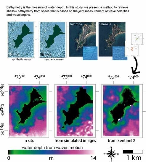
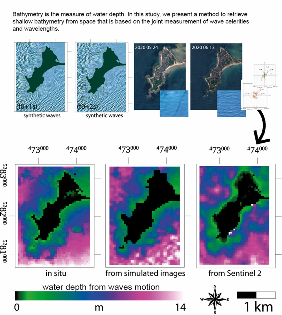
Shallow Bathymetry from Multiple Sentinel 2 Images via the Joint Estimation of Wave Celerity and Wavelength

1
BRGM, French Geological Survey, Direction des Risques et de la Prevention des Risques—3 av. C. Guillemin, 45000 Orleans, France
2
Department of Physical and Environmental Geography, Aristotle University of Thessaloniki, 541 24 Thessaloniki, Greece
*
Author to whom correspondence should be addressed.
Remote Sens. 2021, 13(11), 2149; https://0-doi-org.brum.beds.ac.uk/10.3390/rs13112149
Submission received: 16 April 2021 / Revised: 24 May 2021 / Accepted: 26 May 2021 / Published: 30 May 2021 / Corrected: 30 August 2023
(This article belongs to the Section Ocean Remote Sensing)

Abstract

:
In this study, we present a new method called BathySent to retrieve shallow bathymetry from space that is based on the joint measurement of ocean wave celerity (c) and wavelength (λ). We developed the method to work with Sentinel 2 data, exploiting the time lag between two Sentinel 2 spectral bands, acquired quasi-simultaneously, from a single satellite dataset. Our method was based on the linear dispersion law, which related water depth to wave celerity and wavelength: when the water depth was less than about half the dominant wavelength, the wave celerity and wavelength decreased due to decreasing water depth (h) as the waves propagated towards the coast. Instead of using a best weighted ( c , λ ) fit with the linear dispersion relation to retrieve h, we proposed solving the linear dispersion relation for each ( c , λ ) pair to find multiple h-values within the same resolution cell. Then, we calculated the weighted averaged h-value for each resolution cell. To improve the precision of the final bathymetric map, we stacked the bathymetry values from N-different datasets acquired from the same study area on different dates. We first tested the algorithm on a set of images representing simulated ocean waves, then we applied it to a real set of Sentinel 2 data obtained of our study area, Gâvres peninsula (France, 47°,67 lat.; −3°35 lon.). A comparison with in situ bathymetry yielded good results from the synthetic images (r2 = 0.9) and promising results with the Sentinel 2 images (r2 = 0.7) in the 0–16 m depth zone.

Graphical Abstract

1. Introduction

The retrieval of bathymetry from space is of major importance, particularly in sea areas with shallow depths, where access by conventional methods is tricky, and in areas where shallow morphology changes with time. Many methods based on multispectral imagery exist, which are appropriate in coastal areas where the sea floor can be directly imaged (e.g., [1,2,3,4,5,6] and references therein). In this study, we concentrated only on methods based on ocean wave motion from spaceborne optical imagery. In particular, we concentrated on measurements of wave celerity (c) and wavelength (λ) from quasi-simultaneous image acquisitions. These methods were promising in areas where the water was non-transparent, and they did not require ground calibration.

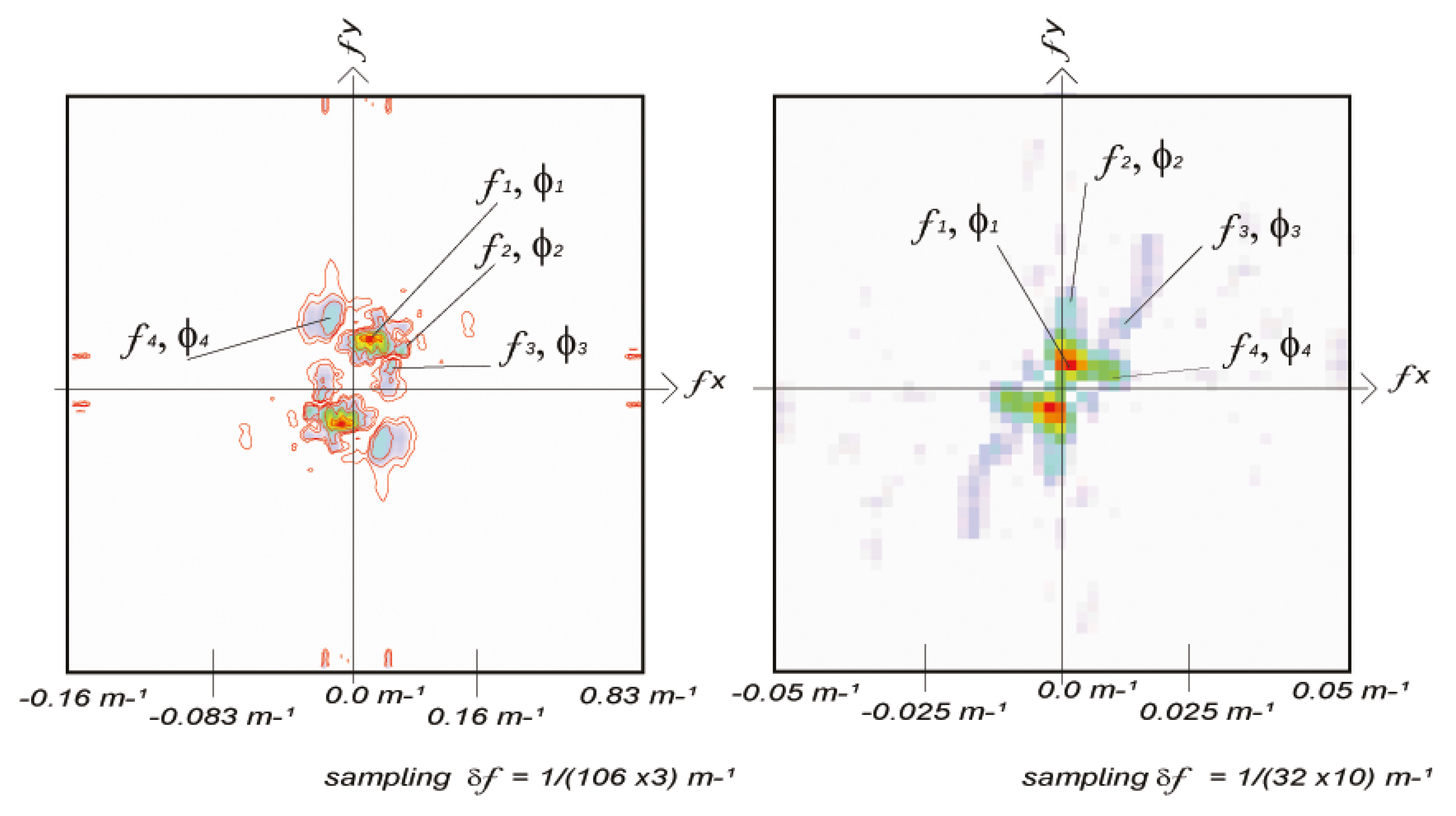
1.1. Theoretical Background

According to linear wave theory [7], when the water depth is less than about half the dominant wavelength, λ, the wave celerity, c, and λ decrease toward the coast due to decreasing water depth. It is then possible to ascertain the water depth from knowledge of the dominant wavelengths and their associated celerities using the linear dispersion relation (also referred to simply as the dispersion relation) for free surface waves (e.g., [8]) [1] as:
h = λ / 2 π   .   tanh 1 ( 2 π c 2 g λ )
where h is the water depth and g is the standard acceleration due to gravity on Earth, equal to 9.81 m/s. Equation (1) was first used in a practical sense during the Second World War [9], and works either with two sequential images acquired within a short time interval (i.e., shorter than the wave period), or with one image but with additional in situ measurements (e.g., [10]).

1.2. Related Works

In this study, we concentrate on spaceborne methods to measure wave celerity and wavelengths from space to retrieve bathymetry. If the reader is interested in other methods, using selective colors absorption for instance, we suggest to read Salameh et al., [11] and the bibliographytherein.
The retrieval of wave celerity from satellites is still challenging today because we need at least two consecutive images acquired with only a few s time delay. Such images can be obtained onboard specific satellites with push-broom sensors. With these sensors, the retrieval of c relies on the non-simultaneous stereo acquisition capability of given platforms, as shown by R. Abileah [12]. Or the information about c can be obtained when two multispectral bands cannot simultaneously exist in the focal plane of the sensor, yielding a de facto short time lag between two bands in the same dataset, allowing one to measure c directly, as proposed by de Michele et al. [13]. With these sensors and the joint measurement of c and λ, h becomes accessible.
In the literature, a few studies have proposed ways to access c and λ from space. For example, Abileah [12] suggested a method to measure c from optical satellite data using Ikonos stereo pairs that had an 11 s time lag. de Michele et al. [13] proposed a method that exploits the small time-lag (2.1 s) between two bands of SPOT-5 data. Danilo and Binet [14] have detailed the concept and limiting factors to access c and λ from space. Based on the aforementioned studies, Poupardin et al. [15,16] proposed a local spectral decomposition method that was employed prior to making celerity estimates to produce local ( c , λ ) pairs that were used to derive the water depth based on the dispersion relation (Equation (1)). Bergsma et al. [17] proposed a method based on multiple Sentinel 2 bands and the Fourier slice theorem. Almar et al. [18] proposed a method to extract bathymetry from the Pleiades satellite’s “persistent” mode, based on ( c , λ ) measures.
Abileah [12], Bergsma et al. [17] and Almar et al. [18] make use of only one ( c , λ ) couple, the most energetic one, to extract one bathymetric value from a resolution cell. In this study, we furthered the work of de Michele et al. [13] and Poupardin et al. [15,16] to retrieve water depth by measuring multiple ( c , λ ) pairs in each resolution cell and we apply it to Sentinel 2 data. The advantages of using Sentinel 2 were manifold. First, the enhanced revisit time (five days) allowed one to improve the data acquisition frequency. Second, the data covered a wide swath, which could be potentially used to map large areas. Third, the data were provided free of charge.

1.3. Our Approach

Our method exploited multiple ( c , λ ) pairs within the same resolution cell. For the purpose of fast processing, we employed two steps: FFT (fast Fourier transform) and the weighted average of multiple h-values within the same resolution cell. First, we used FFT-based methods to produce local, sub-sampled, wave spectra and their associated celerities. To calculate the celerities, we exploited the time lag between two Sentinel-2 bands, acquired during a single Sentinel-2 pass. There are 1.05 s between acquisitions made in band 2 and band 4 (e.g., [19]). Band 2 records sunlight reflected from the Earth surface at the central wavelength of 0.49 μm (perceived as blue by the human eye) and band 4 at 0.68 μm (perceived as red by the human eye). First, we calculate the FFT spectra of these two images. Then, phases and spatial frequencies (i.e., wavenumbers) were combined (Section 2.2) to derive the multiple ( c , λ ) pairs.
The wave spectra were calculated from small sub-images on the basis of a grid defined by the sampling step, where the sampling step defined the resolution of the final bathymetric map. We calculated multiple ( c , λ ) pairs per resolution cell, but instead of using a best weighted ( c , λ ) fit with the linear dispersion relation to retrieve h, we proposed solving the linear dispersion relation for each ( c , λ ) couple. In this way, we found multiple h-values within the same resolution cell. Then, we calculated the weighted average h-value for each resolution cell per dataset, across N datasets. Then, we stacked the results from the N datasets. Because this method was conceived for Sentinel 2, we called it BathySent.
In this study, we tested our procedure on simulated images of waves using n = 6 images. First, from known in situ bathymetry and hydrodynamic modeling, we produced a set of simulated images of waves: a pair of images every 1.05 s, i.e., the time lag between Sentinel 2’s band 2 and band 4. Second, we used the images of the simulated waves along with our BathySent procedure to retrieve the bathymetry. Third, we compared the in situ bathymetry with the ones retrieved by the BathySent method on the simulated dataset. Last, we applied the BathySent procedure to a real Sentinel 2 dataset of the same study area and compared the results.

2. Materials and Methods

2.1. Data

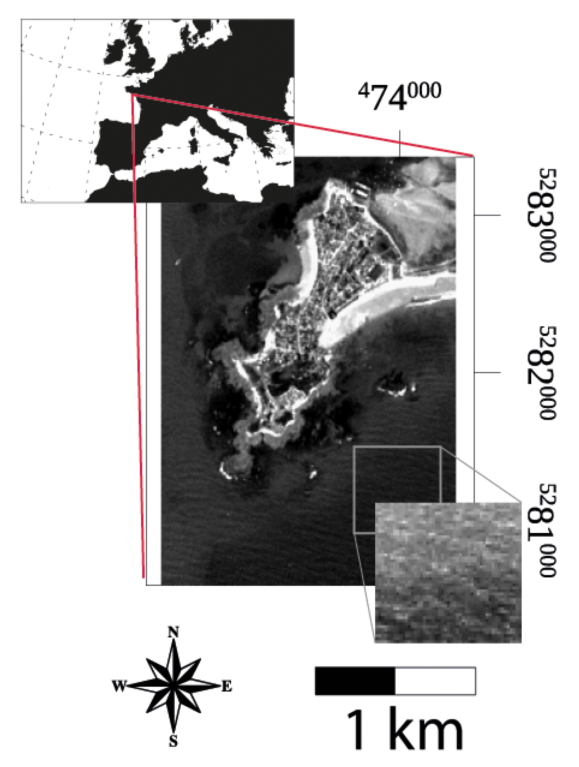
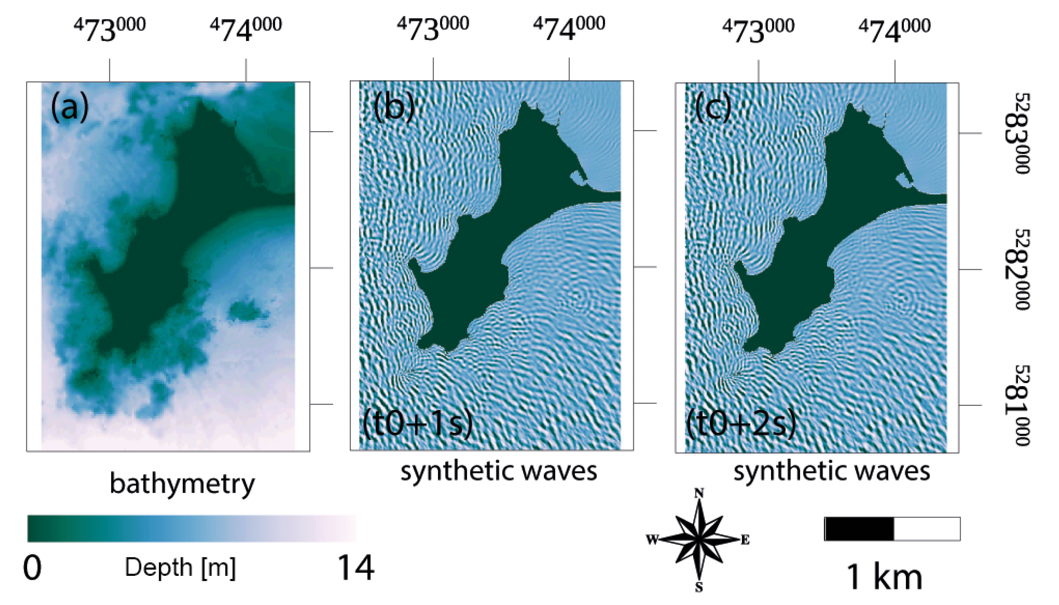
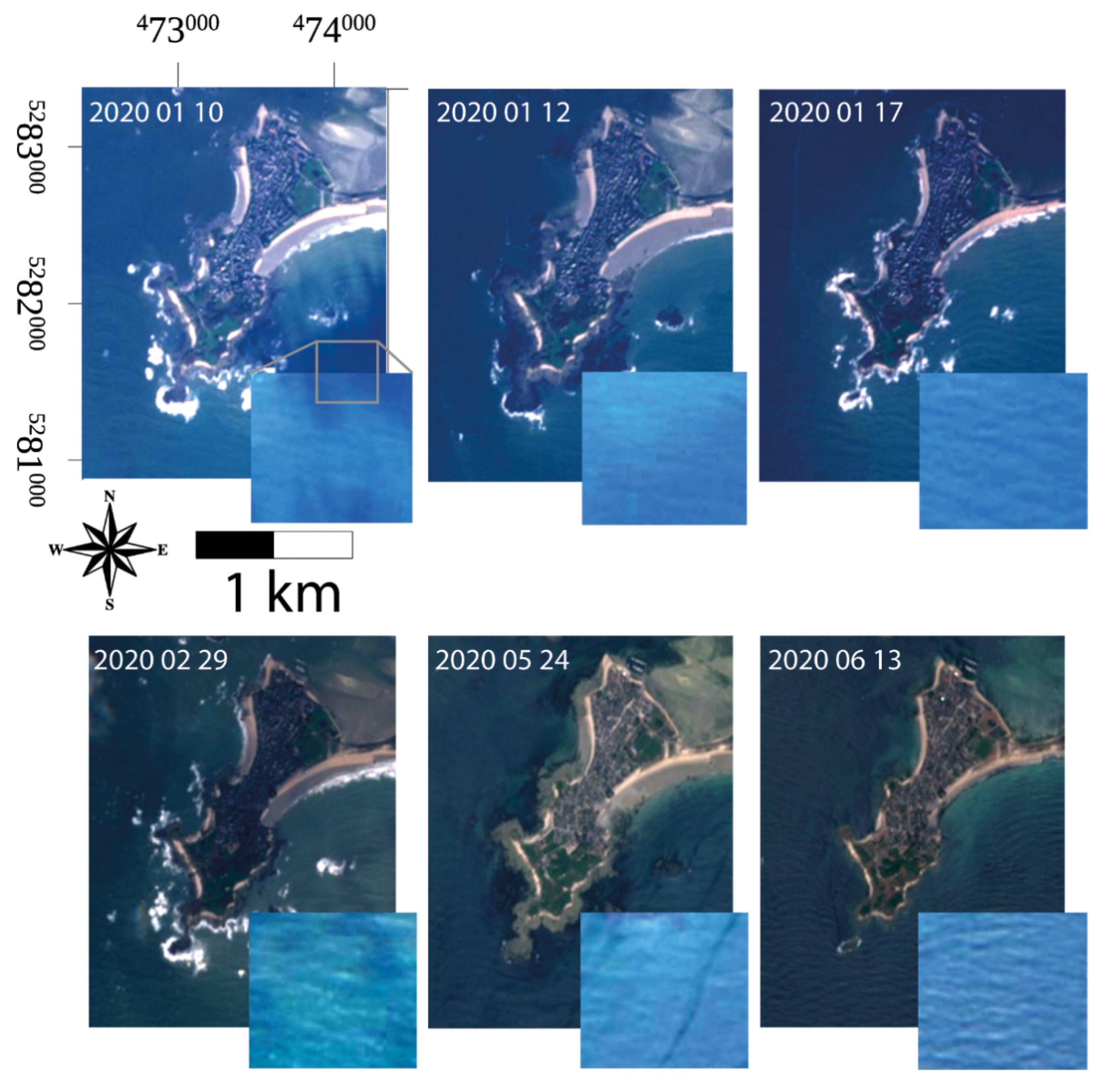
2.1.1. Study Area, in situ Bathymetry, and Simulated Waves

To test our method, we first applied it to simulated images of propagating waves. We simulated the wave propagation using a hydrodynamic model, relying on in situ bathymetry.
Our study area was the Gâvres peninsula, French Atlantic coast, France (Figure 1), which was chosen for two reasons. First, because high-resolution in situ bathymetry, with 3-m spatial resolution, built using in situ surveys (for more details, see Idier et al., [20]) were available. Second, the SWASH model (acronym for simulating waves till shore [21]) was able to simulate waves on a wave-by-wave mode, which was already set-up by the authors of the study area [20]. The study area exhibited many different orientations and bathymetric gradients because of many rocky outcrops.
The model was set up with a horizontal resolution of 3 m and a 10-Hz sampling frequency. The model was previously validated for the study area by reproducing the wave overtopping and induced floods that occurred during the Johanna storm (10 March 2008). In this validation, we used a digital elevation model (DEM) representative of the topography and bathymetry of the area during 2008, built using in situ survey data. More details on the model set up, and the in situ bathymetry, can be found in Idier et al. [20]. We ran the model with the following conditions: still water level of 2 m (NGF-IGN69, the French national vertical datum), offshore 2D JONSWAP wave spectrum [22] characterized by a significant wave height (Hs) of 1 m, peak wave period (Tp) of 6 s, peak wave direction (Dp) of 260° N (nautical convention), and a directional dispersion of 30°. These offshore conditions were propagated to the open boundaries of the SWASH domain using the spectral wave model WW3 [23], such that the boundary conditions of the SWASH simulations were not uniform, and produced realistic local waves. WW3 is solving the random phase spectral action density balance equation for wavenumber-direction spectra (i.e., the wave spectrum), and thus allows estimating the wave spectrum in space and time. These spectra were used as forcing conditions of the non-hydrostatic phase-resolving SWASH model, which, based on these spectra and the still water level, generated a high frequency water level time series that was subsequently used to solve the nonlinear shallow water equations to provide instantaneous water levels in each grid cell (3 m) and at each time step (10 Hz). We created simulations every 1.05 s, each consisting of a set of six images of propagating waves. In Figure 2, we show the in situ bathymetry and two example simulated wave images.

2.1.2. Sentinel 2 MultiSpectral Imager

The European Space Agency’s (ESA) Copernicus Sentinel 2 mission includes two polar-orbiting satellites that monitor the Earth’s surface with a wide swath width (290 km) and high revisit time (10 days at the equator with one satellite, and 5 days with both satellites). Approaching the poles, the revisit time of Sentinel 2 increases where the swaths overlap. When recording a single swath, the Sentinel 2 MultiSpectral Imager (MSI) uses a set of 12 focal plane modules (FPMs) [24]. The key element of being able to measure c relies on the fact that, for technical reasons, multiple CCD bands cannot coexist at the same place in the focal plane of an FPM. Therefore, there is a baseline between two bands due to the difference in the CCD positions, yielding a time lag in image acquisition. The spatial resolution of Sentinel 2’s multispectral (MS) mode in the visible range of the electromagnetic spectrum is 10 m. Therefore, it is able to resolve ocean waves from 20–30 m wavelengths onwards. In this study, we used the time span between MSI bands 2 and 4; that is, 1.05 s. In theory, all resolvable waves and celerities from sentinel 2 can estimate water depth in the study area. We used six level 2C Sentinel 2 images provided orthorectified by ESA for the European Copernicus Program, in the Universal Transverse Mercator (UTM, zone 30 N) reference system. We have displayed the Sentinel 2 images and the acquisition dates, centered on the study area, in Figure 3.

2.2. Methodology

Let us consider a subsection of two MSI bands, normalized by the mean of each subsection amplitude, resulting in two matrices, [A] and [B]. We called this a «window» or resolution cell. Using i and j, we, respectively, identified the columns/lines indices in the window. Over a given window, we computed the two-dimensional discrete fast Fourier transform (DFFT, implemented in NumPy, e.g., [25]) per detector band (matrices [ F A ] and [ F B ] ), where ν and μ were the columns/lines indices in the Fourier domain, respectively. Then, we computed the matrix [R], whose coefficients were given by:
R ν , μ = F A ν , μ F B * ν , μ = Am ν , μ e i θ ν , μ
where ‘*’ represents the complex conjugate and Am is the amplitude of the produced spectrum.
In the module of R ν , μ , we identified multiple peaks, which were considered representative of the most significant waves. Then, we derived their associated wavelengths, λ ν , μ , and phases, θ ν , μ . [A] and [B], being separated in time by 1.05 s, were supposed to have the same spatial frequency content. For this reason, the positions of the peaks in |[R]|, | [ F A ] | , and | [ F B ] | coincided. Therefore, we identified significant wavelengths in [R]. Finally, we determined c by measuring the pixel offset in a wave’s direction of motion ( δ r ν , μ ) between the two bands, which was directly related to the phase of R ν , μ by:
δ r ν , μ = λ ν , μ θ ν , μ 2 π
Then, we obtained c by dividing Equation (3) by δ t k , l , where δ t k , l is the time span between band k and band l.
When the pixel offset was not wavelength-dependent (i.e., r ν , μ = r     ( ν , μ ) ), Equation (3) was equivalent to the phase correlation algorithm used for earthquake-induced ground offset measurements (e.g., [26]). Now, knowing δ t , we utilized the ( λ ν , μ ,     θ ν , μ ) pairs, which were converted to ( λ ν , μ ,   c ν , μ ). The spectral amplitude of R (Am in Equation (2)) was our criterion for selecting the most significant waves in each spectrum (Figure 4), and we kept Am > 0.5 in the normalized spectrum.
Now, we wanted to extract ( c , λ ) pairs to find h. We defined small sampling intervals of equal wavelengths within [R]. Within these sampling intervals, we select values with an [R] amplitude above a given threshold. For each of these values, we extracted the correspondent [R] phases. Then, we estimated the average of these phases, weighted by Am. Proceeding in this manner, we obtained the phases associated with the selected wavelengths, and characterized their significance via their amplitude.
In other words, we defined the smaller possible circular sector of [R] containing the wavelength range [ λ δ λ 2 , λ + δ λ 2 ] . We assumed a nearly constant water depth per FFT window. Therefore, all celerities associated with the circular sector (and thus their phases, as their wavelengths are the same) should be the same. Then, we averaged the [R] phases of all the significant values of [R] included in [ λ δ λ 2 , λ + δ λ 2 ] to deduce an estimate of the pair ( c ,   λ ± δ λ 2 ). δ λ should not exceed the size of few image pixels in order to be sufficiently discriminant. We repeated this operation for the range [ λ δ λ 2 , λ + δ λ 2 ] in [R].
Now that we had all the significant ( c , λ ) pairs, we estimated one value of h for each ( c , λ ) pair by solving the dispersion relation (Equation (1)). Afterwards, we now had one value of h for each ( c ,   λ ) . Here, we took the weighted average of all h-values instead of the best fit to the dispersion relation. This provided us with the final water depth value for a given correlation window or resolution cell, per dataset. The significance of each solution was based on the corresponding amplitude value of [R]. Finally, we corrected each of the N bathymetries for tide offsets and stacked the results into a final bathymetry map. The stacking consists of taking the median value among the six bathymetric maps, for those pixels where there is more than one value. In areas where there is only one value, we keep that value. We propose this way to fill the gaps that might exist if we used one Sentinel 2 image only.

2.3. Correction for Tidal Offsets

A bathymetry is the measure of water depth over the study area at one given date. In this study, we used n = 6 images to estimate six bathymetric maps. Each of the six bathymetries, estimated from Sentinel 2 data, provided the water depth, h, at the time of each image acquisition; i.e., the absolute difference between the sea surface level and the sea bottom. Thus, each bathymetry value was provided with reference to the water level, which was a time-varying quantity. We had to correct this offset and estimated the bathymetry (hcorrected) in a fixed vertical reference frame for each Sentinel 2 acquisition date.
Firstly, we estimated the tide level relative to the mean sea level in our study area using the FES2014 tidal component database [27]. Secondly, we estimated the mean sea level relative to Z = 0 NGF-IGN9 using the data provided by the French Hydrografic Service [28]. Thirdly, we combined this information to estimate the tide level (Ztide) relative to Z = 0 NGF-IGN69 (Table S1, Supplementary Materials). Finally, we subtracted Ztide to total water depth, h, and obtained hcorrected. In the present work, we choose the Z = 0 of the NGF-IGN69 national vertical datum.

3. Results

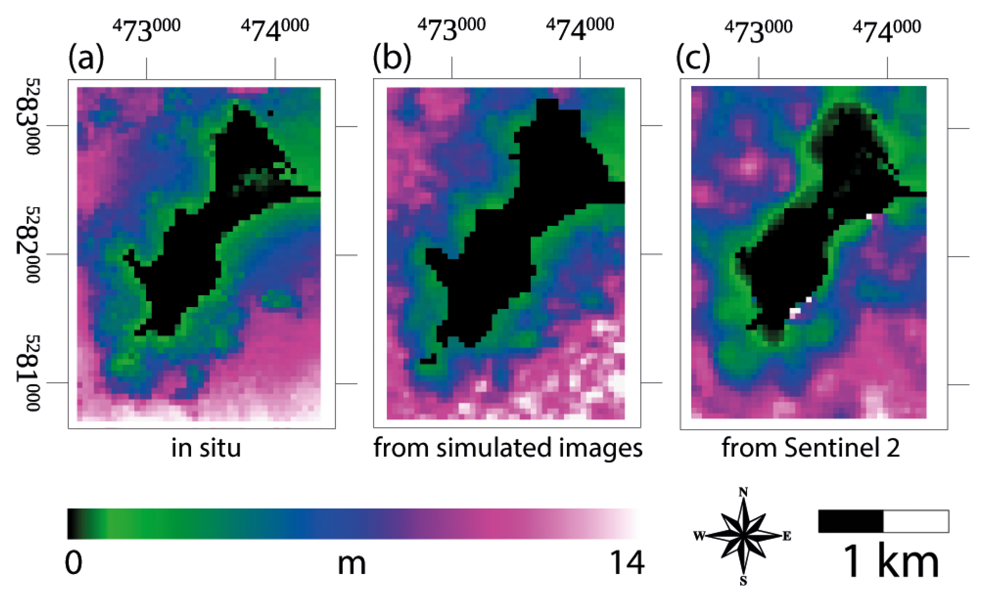
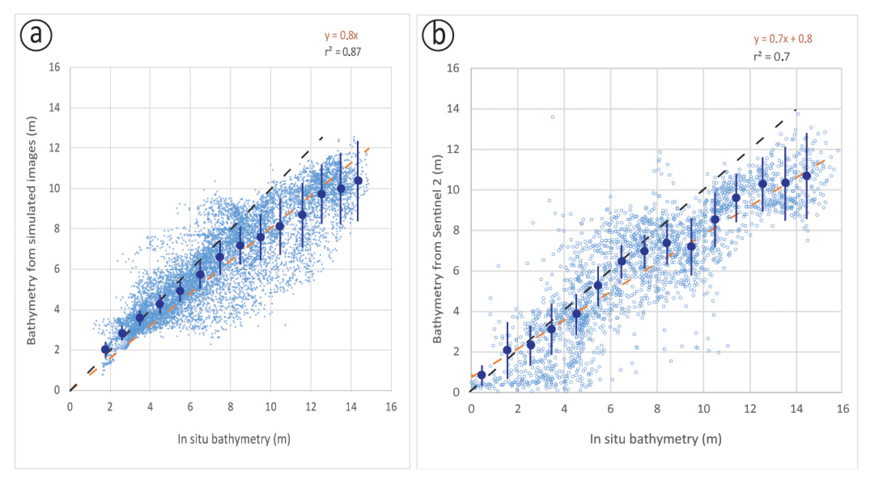
3.1. Results Obtained with the Simulated Dataset

We compiled bathymetry measurements from six simulated wave image couples where each couple had a time lag of 1.05 s and a 3-m pixel size. We used a window size of 32 × 32 pixels, with a sampling interval of 16 pixels. These parameters yielded bathymetry with a 48-m grid resolution. We then calculated the median values of the six bathymetric maps to retrieve an improved map of bathymetry.
Figure 5 shows the in situ bathymetry and the results of the BathySent method applied to the simulated dataset. Our results fit the in situ bathymetry very well (Figure 5a,b). To assess the precision and accuracy of our results, we produced scatterplots of the in situ bathymetry versus the BathySent results, and calculated the coefficient of determination (r2) and the related standard deviation (Figure 6). To do this, we down sampled the in situ bathymetry to the same spatial resolution as the BathySent bathymetry. In the scatterplots shown in Figure 6, we discretized Z into a number of intervals of 1-m width, which center takes the values from 0.5 m to 14.5 m. For each interval, we identified Z (in situ) within that interval, calculated the mean, and identified the geographic location of each point in the interval. At those points precisely, we extracted Z (BathySent), and we calculate the mean of Z (BathySent) and its standard deviation. Then, we plotted the mean Z (in situ) versus the mean Z (Bathysent) along with the root mean square error (RMSE) over the interval as a bar (+/− 0.5 RMSE). The total length of the bar was thus the RMSE. The quantitative comparison between the in situ bathymetry and the bathymetry obtained from the BathySent method yielded r2 = 0.87 with a standard deviation of 2.1 m in the 0–14 m depth zone (Figure 6a). We observe that the BathySent algorithm systematically underestimated deeper values. We provided an explanation in the discussion section.
The BathySent bathymetry shown in Figure 5b was coarser with respect to the in situ bathymetry seen in Figure 2a. The sampling step of our methodology yielded a final map whose pixel size was 16 times larger than the original image pixel size. Nevertheless, we can see from Figure 5a,b that the shapes of bathymetric features was generally representative of the geomorphology of the in situ bathymetry. Therefore, we deduced that in extremely favorable conditions, such as the ones present in this exercise (where, for instance, the still water level was known), our methodology is reliable.

3.2. Results with Sentinel 2

We chose to use the Sentinel 2, level 1C archive from 2020. Among all the data in the ESA SciHub archive, many contain clouds, and many others do not contain images of waves. As a result, we used six Sentinel 2 datasets (Figure 3) to produce six bathymetry maps with the BathySent method for the study area. For each image, we used a moving window of 32 × 32 pixels (320 m) with a sampling interval of 16 pixels (160 m). A too-large window would imply a decrease in spatial resolution of the results; hence, 320 m was well within the maximum wavelength expected in this area.
The results of applying the BathySent method to real Sentinel 2 data are shown in Figure 5c. We showed that our method estimated bathymetry for most of the study area. The measurements were quite scattered, but they represented a sound and valuable first-level information when bathymetry was unknown in a given area. Quantitatively, the comparison between the in situ bathymetry and the BathySent bathymetry yielded an r2 = 0.7 and a standard deviation of 1.5 m (Figure 6b). Moreover, there is a tendency for the BathySent algorithm to underestimate deeper values. Qualitatively, we showed that the spatial patterns were preserved, but they were not always represented in high fidelity. We interpreted this as the result of the coarser resolution of the bathymetry values retrieved with Sentinel 2 (160 m grid) with respect to the ones retrieved from the synthetic images (48 m grid).

4. Discussion

We tested the BathySent algorithm to retrieve bathymetry from both simulated and Sentinel 2 images. Firstly, we chose a study area where bathymetry was known from in situ measurements. We started with testing the algorithm on a series of simulated images of waves, to retrieve the known input bathymetry, and the results of the tests were very good in terms of r2 (>0.8). Next, we applied the algorithm to six real Sentinel 2 images and retrieved six bathymetry maps for the study area. Finally, we stacked the six bathymetry maps to improve the final precision. The process of stacking multiple data and the use of multiple Sentinel 2 images aimed at filling the potential gaps in the final bathymetry map. To evaluate the accuracy in this study, our strategy was not to look at each single bathymetry map but to compare the stacked bathymetry map to in situ bathymetry.
The results from the synthetic images proved that our method was able to retrieve bathymetry at least up to a 16-m depth in the study area. A quantitative comparison between our results and in situ bathymetry showed that our method was able to retrieve bathymetry throughout most of the study area, with a standard deviation of 1.5 m and an r2 = 0.7. This r2 result indicated higher dispersion with respect to the synthetic test, which was likely due to a tendency for the BathySent algorithm to underestimate deeper values. This systematic under-estimate of deeper value was expected. It is due principally to two factors. According to equation [1], to extract deeper bathymetry values we would need either very large wavelengths or short wavelengths but a very precise c (precise to the 0.01 m/s). Therefore, given that the maximum nominal precision that we can get on c is 1/10th of the image pixel size, deeper bathymetry values rely on the presence of large wavelengths in the scene (Figure 7). In fact, when we solve Equation (1) if c is overestimated h = nan (not a number). If c is underestimated, h = real but underestimated.
As highlighted by Poupardin et al. [15], the quality of c measurements is a key factor in analyses such as presented here. For instance, for a wavelength of 32 m and a celerity of 6 m/s, an error of 0.6 m/s (i.e., 10%) would contribute to a relative error of 42% in the bathymetry. Based on published studies of image correlations with FFT methods (e.g., [26]) we can assume that the precisions of the measured values of c vary between 1/4 and 1/10 the pixel size divided by the time span, depending on the image noise (i.e., between 1 and 2.5 m/s for Sentinel 2). With a smaller pixel size, we could obtain more precise values of c, which in turn would allow more accurate water depth estimations for the same λ . The minimum theoretical detectable λ is twice the pixel size (i.e., 20 m for Sentinel 2), limiting the possibility of investigating short wavelengths in small sub-images close to the shore. In addition, shorter λ s are less sensitive to deeper bathymetry than larger λ s (Figure 7). Therefore, the theoretical resolution of the final bathymetric map is expected to decrease with depth as the detection of larger λ s requires larger sub-images. In principle, an optimal algorithm—in terms of final spatial resolution and precision—should be able to simultaneously analyze short and long wavelengths in the image to address these issues.
In the present study, the effect of tidal currents on Sentinel 2 wave celerity is neglected, because it is very small with respect to Sentinel 2 pixel size. Indeed, in the study area, at the exact time of Sentinel 2 image acquisitions, the depth averaged currents—induced by the tide, atmospheric pressure and wind—are estimated by the Ifremer (Institut Français de Recherche pour l’Exploitation de la Mer) MARC service (Modélisation et Analyse pour la Recherche Côtière, [29]) to be lower than 0.1 m/s.
The use of the high revisit time and fully available archive of Sentinel 2 was key for selecting multiple images that fulfilled all the requirements described above, which in turn encompassed a diversity of conditions in terms of wave conditions (wavelengths, directions, and visibility in the images) and sensors characteristics (resolution and time spans).

5. Conclusions

In conclusion, this study confirmed the potential use of multispectral images obtained by Sentinel 2 for shallow bathymetry mapping and it demonstrated the reliability of the BathySent concept.
The high revisit time of Sentinel 2 allowed us to use multiple images without clouds and with visible ocean waves. This point was key to fill the gaps in the bathymetry map that would appear inevitably if we used only one image.
The method has a tendency to underestimate deeper values. This is due to the limit in the precision of c for the range of λ s in the study area when we solve the linear dispersion Equation (1). The precision on c depends on the pixel size and on the time lag. Therefore, we conclude that combination of multiple satellite missions, including the VENμS mission [30], Pléiades and SPOT, with a diverse range of pixel sizes and time lags, must be foreseen.

Supplementary Materials

The following are available online at https://0-www-mdpi-com.brum.beds.ac.uk/2072-4292/13/11/2149/s1: Table S1: Acquisition dates; tide correction; Sentinel 2 bands used; time lags between bands

Author Contributions

Conceptualization, M.d.M. and D.R.; methodology, M.d.M., D.R. and D.I.; validation, M.d.M., D.I., D.R., and M.F.; formal analysis, M.d.M., D.R., D.I. and F.S.; coding F.S., D.R. and M.d.M.; writing—original draft preparation, D.R., M.d.M., D.I., M.F. and F.S. All authors have read and agreed to the published version of the manuscript.

Funding

This research has been funded by the European Space Agency and BRGM under the EO Science for Society Permanently Open Call, contract No. 4000124021.

Institutional Review Board Statement

Not applicable.

Informed Consent Statement

Not Applicable.

Data Availability Statement

The data presented in this study are available on request from the corresponding author.

Acknowledgments

This project has been funded by the European Space Agency and BRGM under the EO Science for Society Permanently Open Call, contract No. 4000124021. We acknowledge the French Agence Nationale pour la Recherche (ANR) for funding the RISCOPE project (ANR-16-CE04-0011) for providing the in situ bathymetry, the tide data, and the simulated wave images based on hydrodynamic modeling. We are thankful to Faiza Boulahya at BRGM, Espen Volden and Ferran Gascon at ESA. We thank 4 anonymous reviewers for their suggestions.

Conflicts of Interest

The authors declare no conflict of interest.

References

  1. Lyzenga, D.R. Remote sensing of bottom reflectance and water attenuation parameters in shallow water using aircraft and Landsat data. Int. J. Remote Sens. 1981, 2, 71–82. [Google Scholar] [CrossRef]
  2. Lyzenga, D.R. Shallow-water bathymetry using combined lidar and passive multispectral scanner data. Int. J. Remote Sens. 1985, 6, 115–125. [Google Scholar] [CrossRef]
  3. Feigels, J. LiDARs for oceanological research: Criteria for comparison, main limitations, perspectives. Ocean Opt. 1992, 1750, 473–484. [Google Scholar]
  4. Stumpf, R.P.; Holderied, K.; Sinclair, M. Determination of water depth with high-resolution satellite imagery over variable bottom types. Limnol. Oceanogr. 2003, 48, 547–556. [Google Scholar] [CrossRef]
  5. Lyzenga, D.; Malinas, N.; Tanis, F. Multispectral bathymetry using a simple physically based algorithm. IEEE Trans. Geosci. Remote. Sens. 2006, 44, 2251–2259. [Google Scholar] [CrossRef]
  6. Caballero, I.; Stumpf, R.P. Towards routine mapping of shallow bathymetry in environments with variable turbidity: Contribution of Sentinel 2A/B satellites mission. Remote Sens. 2020, 12, 451. [Google Scholar] [CrossRef]
  7. Airy, G.B. Tides and waves. Encyclopaedia Metropolitana (1817–1845), Mixed Sciences. In Trigonometry, On the Figure of the Earth, Tides and Waves; Rose, H.J., Ed.; London, UK, 1841; Volume 3, 396p. [Google Scholar]
  8. Phillips, O.M. The Dynamics of the Upper Ocean; Cambridge University Press: Cambridge, UK, 1977; pp. 1–336. [Google Scholar]
  9. Williams, W.W. The Determination of Gradients on Enemy-Held Beaches. Geogr. J. 1947, 109, 76. [Google Scholar] [CrossRef]
  10. Danilo, C.; Melgani, F. Wave Period and Coastal Bathymetry Using Wave Propagation on Optical Images. IEEE Trans. Geosci. Remote Sens. 2016, 54, 6307–6319. [Google Scholar] [CrossRef]
  11. Salameh, E.; Frappart, F.; Almar, R.; Baptista, P.; Heygster, G.; Lubac, B.; Raucoules, D.; Almeida, L.P.; Bergsma, E.W.J.; Capo, S.; et al. Monitoring Beach Topography and Nearshore Bathymetry Using Spaceborne Remote Sensing: A Review. Remote Sens. 2019, 11, 2212. [Google Scholar] [CrossRef]
  12. Abileah, R. Mapping shallow water depth from satellite. In Proceedings of the ASPRS Annual Conference, San Carlos, CA, USA, 1–5 May 2006; pp. 1–7. [Google Scholar]
  13. de Michele, M.; Leprince, S.; Thiébot, J.; Raucoules, D.; Binet, R. Direct measurement of ocean waves velocity field from a single SPOT-5 dataset. Remote Sens. Environ. 2012, 119, 266–271. [Google Scholar] [CrossRef]
  14. Danilo, C.; Binet, R. Bathymetry estimation from wave motion with optical imagery: Influence of acquisition parameters. In Proceedings of the 2013 MTS/IEEE OCEANS conference, Bergen, Norway, 10–13 June 2013; pp. 1–5. [Google Scholar]
  15. Poupardin, A.; Idier, D.; De Michele, M.; Raucoules, D. Water Depth Inversion from a Single SPOT-5 Dataset. IEEE Trans. Geosci. Remote Sens. 2016, 54, 2329–2342. [Google Scholar] [CrossRef]
  16. Poupardin, A.; De Michele, M.; Raucoules, D.; Idier, D. Water depth inversion from satellite dataset. In Proceedings of the 2014 IEEE Geoscience and Remote Sensing Symposium, Quebec City, QC, Canada, 13–18 July 2014; pp. 2277–2280. [Google Scholar]
  17. Bergsma, E.W.J.; Almar, R.; Maisongrande, P. Radon-Augmented Sentinel-2 Satellite Imagery to Derive Wave-Patterns and Regional Bathymetry. Remote Sens. 2019, 11, 1918. [Google Scholar] [CrossRef]
  18. Almar, R.; Bergsma, E.W.; Maisongrande, P.; de Almeida, L.P.M. Wave-derived coastal bathymetry from satellite video imagery: A showcase with Pleiades persistent mode. Remote. Sens. Environ. 2019, 231, 111263. [Google Scholar] [CrossRef]
  19. Yurovskaya, M.; Kudryavtsev, V.; Chapron, B.; Collard, F. Ocean surface current retrieval from space: The Sentinel-2 multispectral capabilities. Remote Sens. Environ. 2019, 234, 111468. [Google Scholar] [CrossRef]
  20. Idier, D.; Rohmer, J.; Pedreros, R.; Le Roy, S.; Lambert, J.; Louisor, J.; Le Cozannet, G.; Le Cornec, E. Coastal flood: A composite method for past events characterisation providing insights in past, present and future hazards—joining historical, statistical and modelling approaches. Nat. Hazards 2020, 101, 465–501. [Google Scholar] [CrossRef]
  21. Zijlema, M.; Stelling, G.; Smit, P. SWASH: An operational public domain code for simulating wave fields and rapidly varied flows in coastal waters. Coast. Eng. 2011, 58, 992–1012. [Google Scholar] [CrossRef]
  22. Hasselmann, K.; Olbers, D. Measurements of wind-wave growth and swell decay during the Joint North Sea Wave Project (JONSWAP). Ergaenzungsheft Dtsch. Hydrogr. Z. Reihe A 1993, 12, 1–95. [Google Scholar]
  23. Ardhuin, F.; Rogers, W.; Babanin, A.; Filipot, J.-F.; Magne, R.; Roland, A.; Van Der Westhuysen, A.; Queffeulou, P.; Lefevre, J.-M.; Aouf, L.; et al. Semiempirical Dissipation Source Functions for Ocean Waves. Part I: Definition, Calibration, and Validation. J. Phys. Oceanogr. 2010, 40, 1917–1941. [Google Scholar] [CrossRef]
  24. Suhet, H.B. Sentinel-2 User Handbook. ESA Standard Document. Issue 1. Revision 1; European Space Agency (ESA), 2015. Available online: https://earth.esa.int/web/sentinel/user-guides/sentinel-2-msi (accessed on 3 May 2019).
  25. Harris, C.R.; Millman, K.J.; Van Der Walt, S.J.; Gommers, R.; Virtanen, P.; Cournapeau, D.; Wieser, E.; Taylor, J.; Berg, S.; Smith, N.J.; et al. Array programming with NumPy. Nature 2020, 585, 357–362. [Google Scholar] [CrossRef]
  26. Van Puymbroeck, N.; Michel, R.; Binet, R.; Avouac, J.-P.; Taboury, J. Measuring earthquakes from optical satellite images. Appl. Opt. 2000, 39, 3486–3494. [Google Scholar] [CrossRef]
  27. Carrere, L.; Lyard, F.; Cancet, M.; Guillot, A.; Picot, N. FES 2014, a new tidal model Validation results and perspectives for improvements. In Proceedings of the ESA Living Planet Symposium, Prague, Czech Republic, 9–13 May 2016. [Google Scholar]
  28. SHOM. Références Altimétriques Maritimes; SHOM publishing: Brest, France, 2017; ISBN 978-2-11-139469-8. [Google Scholar]
  29. Ardhuin, F. 2021. Available online: https://marc.ifremer.fr/resultats/courants/modeles_mars3d_manche_gascogne (accessed on 1 February 2021).
  30. Bergsma, E.W.; Almar, R.; Rolland, A.; Binet, R.; Brodie, K.L.; Bak, A.S. Coastal morphology from space: A showcase of monitoring the topography-bathymetry continuum. Remote Sens. Environ. 2021, 261, 112469. [Google Scholar] [CrossRef]
Figure 1. Study area and an example Sentinel 2 sub-image (band 4). The square represents a histogram-stretched cut of the image, highlighting the waves therein. Coordinates are expressed in UTM N30.
Remotesensing 13 02149 g001
Figure 2. (a) In situ bathymetry. (b,c) two examples of simulated wave images, shaded from simulated waves height. The solar azimuth and zenith angles used for shading are standard values (45°, 45°). Coordinates are expressed in UTM N30.
Remotesensing 13 02149 g002
Figure 3. Sentinel 2 dataset centered on the study area and acquisition dates. Color composite with bands 4, 3, 2 displayed as red, blue and green. The grey square presents a closer look image to show how Sentinel 2 recorded waves on different dates. The close-up image colors are enhanced by histogram-stretching for the purpose of visualization. Coordinates are expressed in UTM N30.
Remotesensing 13 02149 g003
Figure 4. FFT spectra of the simulated waves (left) and Sentinel 2 waves (right). Size of the FFT window in this example: 106 pixels for the simulated waves and 32 pixels for Sentinel 2. ( c , λ ) couples are here represented as (f,   Φ ) couples; f is the FFT frequency—proportional to λ - and Φ is the FFT phase that we used to calculate c .
Remotesensing 13 02149 g004
Figure 5. (a) In situ bathymetry, (b) bathymetry retrieved from the simulated waves, and (c) bathymetry retrieved from Sentinel 2. The land masks in (b,c) were bigger than in (a) because the correlation window of 32 × 32 pixels, associated with a sampling step of 16 pixels, yielded a decrease in the spatial resolution. Each bathymetric map is provided in the NGF-IGN69 vertical reference frame.
Remotesensing 13 02149 g005
Figure 6. (a) Scatterplot of the in situ bathymetry versus the bathymetry from the simulated waves. (b) Scatterplot of the in situ bathymetry versus the bathymetry from Sentinel 2.The dark blue dots represent the mean value per bin, and the blue bars represent the RMSE per bin; please see the main text for further explanations. The dark dotted line represents the 1:1 correlation line. The orange dotted line represents the linear fit to the data, the best-fitting equation of which is located at top of the graph, along with the corresponding r2 value.
Remotesensing 13 02149 g006
Figure 7. Example of the h dependency on c and λ for five values of λ, from Equation (1). It can be seen that the precision of the measured celerity was much more critical than the wavelength.
Remotesensing 13 02149 g007
Publisher’s Note: MDPI stays neutral with regard to jurisdictional claims in published maps and institutional affiliations.

