
Sea Ice Concentration Products over Polar Regions with Chinese FY3C/MWRI Data

1
National Satellite Ocean Application Service, Beijing 100081, China
2
Key Laboratory of Space Ocean Remote Sensing and Application, MNR, Beijing 100081, China
3
Zhuhai Orbita Aerospace Science & Technology Co., Ltd., Zhuhai 519080, China
4
Independent Researcher, Mailbox No. 5111, Beijing 100094, China
*
Author to whom correspondence should be addressed.
Remote Sens. 2021, 13(11), 2174; https://0-doi-org.brum.beds.ac.uk/10.3390/rs13112174
Submission received: 28 April 2021
/
Revised: 28 May 2021
/
Accepted: 29 May 2021
/
Published: 2 June 2021
(This article belongs to the Special Issue Remote Sensing Monitoring of Arctic Environments)
Abstract
:Polar sea ice affects atmospheric and ocean circulation and plays an important role in global climate change. Long time series sea ice concentrations (SIC) are an important parameter for climate research. This study presents an SIC retrieval algorithm based on brightness temperature (Tb) data from the FY3C Microwave Radiation Imager (MWRI) over the polar region. With the Tb data of Special Sensor Microwave Imager/Sounder (SSMIS) as a reference, monthly calibration models were established based on time–space matching and linear regression. After calibration, the correlation between the Tb of F17/SSMIS and FY3C/MWRI at different channels was improved. Then, SIC products over the Arctic and Antarctic in 2016–2019 were retrieved with the NASA team (NT) method. Atmospheric effects were reduced using two weather filters and a sea ice mask. A minimum ice concentration array used in the procedure reduced the land-to-ocean spillover effect. Compared with the SIC product of National Snow and Ice Data Center (NSIDC), the average relative difference of sea ice extent of the Arctic and Antarctic was found to be acceptable, with values of −0.27 ± 1.85 and 0.53 ± 1.50, respectively. To decrease the SIC error with fixed tie points (FTPs), the SIC was retrieved by the NT method with dynamic tie points (DTPs) based on the original Tb of FY3C/MWRI. The different SIC products were evaluated with ship observation data, synthetic aperture radar (SAR) sea ice cover products, and the Round Robin Data Package (RRDP). In comparison with the ship observation data, the SIC bias of FY3C with DTP is 4% and is much better than that of FY3C with FTP (9%). Evaluation results with SAR SIC data and closed ice data from RRDP show a similar trend between FY3C SIC with FTPs and FY3C SIC with DTPs. Using DTPs to present the Tb seasonal change of different types of sea ice improved the SIC accuracy, especially for the sea ice melting season. This study lays a foundation for the release of long time series operational SIC products with Chinese FY3 series satellites.
1. Introduction
Polar sea ice affects the atmosphere and ocean circulation and plays an important role in global climate change [1]. The existence of sea ice modifies the heat exchange between the atmosphere and the ocean, affects the heat balance of the ocean, and hinders momentum transfer between the atmosphere and the ocean. Compared with open water, the albedo of sea ice is greater, sea ice reflects more solar radiation back to the space and absorbs less shortwave radiation. In particular, the extent of sea ice changes greatly throughout the year and seasonally and has an important impact on the global climate system [2]. With global warming, satellite observations show that Arctic sea ice has been declining in extent, thickness, and volume since 1979 [3] and Antarctic sea ice has shown a trend of increasing yearly [4]. On 16 September 2012, Arctic sea ice reached its minimum extent of 3.4 × 10⁶ km2 since modern satellite measurements became available in 1979, which is only 55% of the 1981–2010 average of 6.2 × 10⁶ km2 [5]. The change in polar sea ice is a pressing issue in the international community, necessitating further optimization of the accuracy of sea ice datasets, the continuity of time series, and the consistency of spatial resolution.
The parameters that can reflect the change in sea ice include sea ice concentration (SIC), sea ice extent (SIE), sea ice area (SIA), ice age, and ice thickness. The variation in sea ice is closely related to temperature, wind field, sea water temperature, and salinity. Among the key parameters, the SIC can reflect the spatial distribution characteristics of sea ice. It is defined as the areal fraction of sea ice over a given region. With this parameter, we can further obtain information on the SIE and SIA over a special region. The SIC can be used as the input parameter for atmospheric and oceanic predictions and climate models [6]. Passive microwave (PM) radiometers on satellites are effective tools to obtain all-weather, near-real-time, and long-term continuous SIC data over polar regions. The National Snow and Ice Data Center (NSIDC) has provided SIC data over the Antarctic and Arctic since 1978 with the brightness temperature (Tb) measured by the Scanning Multichannel Microwave Radiometer (SMMR) on the satellite Nimbus-7 [7], the Special Sensor Microwave Imager (SSM/I) on the satellite’s Defense Meteorological Satellite Program (DMSP) F8, F11, and F13, and the Special Sensor Microwave Imager/Sounder (SSMIS) on the satellites DMSP F17 and F18. The Advanced Microwave Scanning Radiometer 2 (AMSR2) aboard Global Change Observation Mission 1-Water (GCOM-W1) can be used to complement the time series. NSIDC has become one of the main data sources for global climate change research and polar prediction models. According to a report in Nature [8], F19 was launched in 2014 but experienced sensor problems in 2016. SSMIS on F18 and AMSR2 in orbit are out of service, and there is no subsequent launch plan. The unlaunched F20 is still in storage. The continuous record of SIC data lasting nearly 40 years is in danger of being broken. The observation frequency bands of China’s HaiYang 2 (HY-2) and FengYun 3 (FY-3) series satellite PM radiometers are similar to that of the SSMIS on the DMSP satellites; thus, these instruments have the potential to become the main data source of polar sea ice observations.
In this study, we developed an intersensor calibration of the Tb between the Microwave Radiation Imager (MWRI) on FY3C and the SSMIS on F17, and we systematically evaluated the temporal continuity of the daily SIC products over the polar region from FY3C/MWIR data. In Section 2, the data used in this study and the preprocessing method are introduced. Then, the intersensor calibrations of Tb are described in Section 3. Section 4 presents the SIC retrieval methods, which include the fixed tie points (FTPs) NASA team (NT) method and the dynamic tie points (DTPs) NT method. The SIC product of FY3C/MWIR is compared with the SIC of NSIDC in Section 5 and evaluated with the ship observation data, synthetic aperture radar (SAR) sea ice cover product, and Round Robin Data Package (RRDP) in Section 6. Section 7 describes the SIC dataset based on the proposed method of this study. The conclusions are summarized in Section 8.
2. Data and Preprocessing
2.1. Brightness Temperature Data
On 23 September, 2013, the Chinese meteorological satellite FY3C was successfully launched, with a microwave scanning radiometer named MWRI to provide operational global Tb data [9]. MWRI has five frequencies (10.65 GHz, 18.7 GHz, 23.8 GHz, 36.5 GHz, and 89 GHz) and two polarization modes of vertical polarization (V) and horizontal polarization (H). The conical scanning mode with a 45° scanning angle was adopted, and the swath width is 1400 km, including 254 scanning data with each line. The ground resolution of the channels, from low frequency to high frequency, is 51 × 85, 30 × 50, 27 × 45, 18 × 30, and 9 × 15 km [10]. The level 1B data of MWRI are used in this study, which are stored in HDF format and include longitude, latitude, and 10 bands of Tb [11].
SSMIS, onboard DMSP F17, was launched on 4 November 2006. The flight altitude is 850 km, the inclination angle is 98.8°, the orbit cycle is 102 min, and the transit time of the ascending intersection is approximately 5:31 pm. The SSMIS sensor measures the microwave energy at 24 frequencies from 19 to 183 GHz, and the swath width is 1700 km [12]. The SSMIS data used in this research were downloaded from the Remote Sensing System website [13,14]. These data have been calibrated with SSM/I, WindSat, and Advanced Microwave Scanning Radiometer for EOS (AMSR-E) and can be used for interannual and interdecadal trend research. The data are in NC format, including the bright temperature data of five bands including 19V, 19H, 22V, 37V, and 37H.
The FY3C/MWIR Tb data of 18.7 GHz, 23.8 GHz, and 36.5 GHz are radiometrically corrected with the Tb data of the similar bands from F17/SSMIS. The radiometric parameters of these two sensors are listed in Table 1.
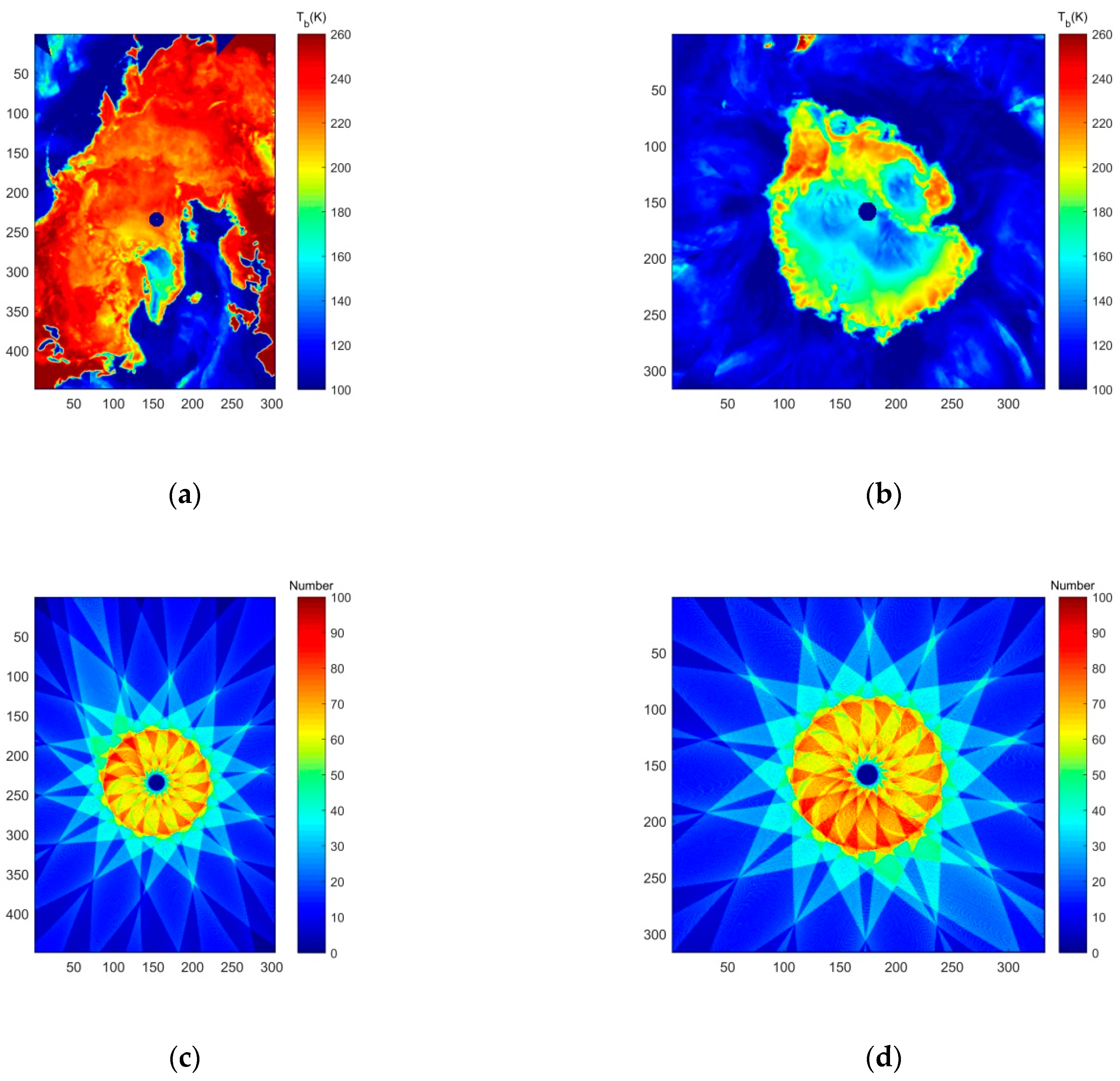
Before the ntersensory calibration between SSMIS and MWRI and SIC retrieval, the daily 14 tracks of Tb data of SSMIS and MWRI were reconstructed to a polar plane grid using polar stereographic projection formulae. The projection plane was specified by NSIDC to Earth’s surface at 70 degrees northern and southern latitude with little or no distortion in the marginal ice zone [15,16]. After projection with a 25 km spatial resolution, the grid sizes of the Arctic and Antarctic are 448 × 304 and 332 × 316, respectively (see Figure 1). Figure 1c,d reflect the observation times of each pixel of the polar plane grid obtained by resampling, which is distributed within 0–100, and most of the areas are mainly concentrated within 20–70.
2.2. Evaluation Data
2.2.1. SIC Product of NSIDC
The SIC operational products provided by the NSIDC [17] were compared with the result retrieved with FY3C data. The dataset includes the daily and monthly average SICs in the Arctic and Antarctic since 26 October 1978. The data are in binary bin format with a spatial resolution of 25 km. The data used in this study were generated with SSMIS data from DMSP F17 through the NASA team algorithm developed by the NASA Goddard Space Flight Center (GSFC).
2.2.2. ASPeCt Ship Observation Data
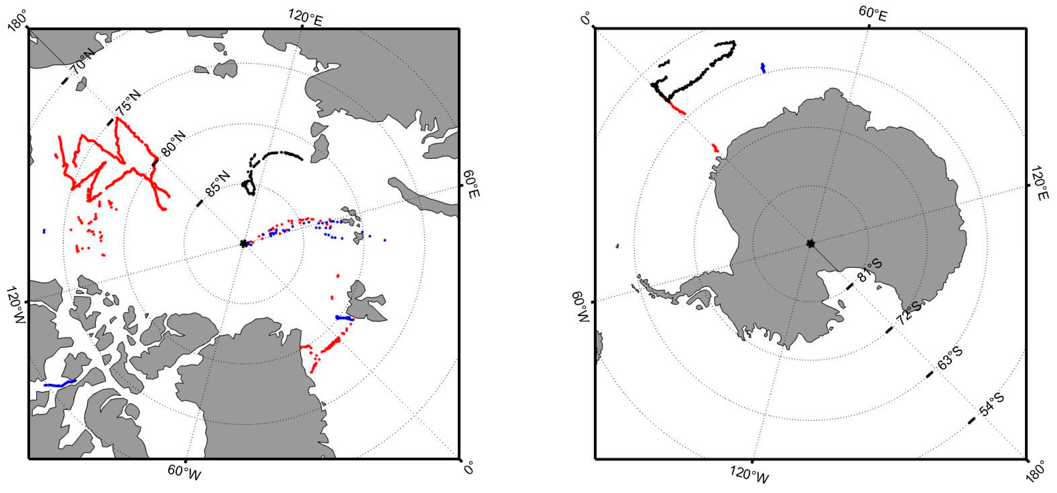
Ship observation data over the North and South poles from 2016 to 2019 were collected, mainly from the Pangaea website [18] and the 7th and 8th Chinese National Arctic Research Expedition (CHINARE). Ship observation primarily refers to the international standard of sea ice visual observation, Antarctica sea ice processes and climate (ASPeCt) [19], which comprises hourly observation of sea ice, usually including SIC, sea ice type, sea ice thickness, and other information. This paper uses observed total SIC (OBS SIC), which is estimated in steps of 10%, as the true value of SIC. Figure 2 shows the geographical distribution of the observation data, including 1220 Arctic observation data and 355 Antarctic observation data.
2.2.3. SAR Data
Wang and Li (2020) [20] developed a modified U-Net deep learning network method for deriving a sea ice cover product for the Arctic using Sentinel-1 (S1) dual-polarization data in extrawide (EW) swath mode. With the above method, they supplied sea ice cover products at 400 m spatial resolution with over 28,000 S1 EW images acquired in 2019 [21]. We collected 322 SAR sea ice cover products on the first day of each month of 2019. By counting the number of sea ice cover pixels in each 25 × 25 km grid, we obtained SIC data with a spatial resolution of 25 km and then evaluated the SIC products of FY3C and NSIDC.
2.2.4. RRDP Data
RRDP v2.2.1 [22] was used as the ground truth to evaluate the uncertainty of FY3C’s SIC. RRDP contains the locations of high-latitude open water (OW, 0% SIC) and closed ice (CI, 100% SIC) for the period 2007–2016. The OW dataset contains the location and valid period (specific months of summer and winter) for open water data points of the Northern Hemisphere and Southern Hemisphere. The CI dataset contains the location and specific date of nominal 100% sea ice based on the ice drift dataset from SAR. Compared with the OW data and CI data, the FY3C SIC product of 2016 was used to compute the uncertainty based on the evaluation method of Lavergne et al. (2019) [23].
3. Intersensor Calibrations between SSMIS and MWRI
To ensure the consistency of long time series data records, the observations of different instruments need to be calibrated to a single benchmark [24]. In this study, intersensor calibrations were performed between the Tbs from the SSMIS and MWRI.
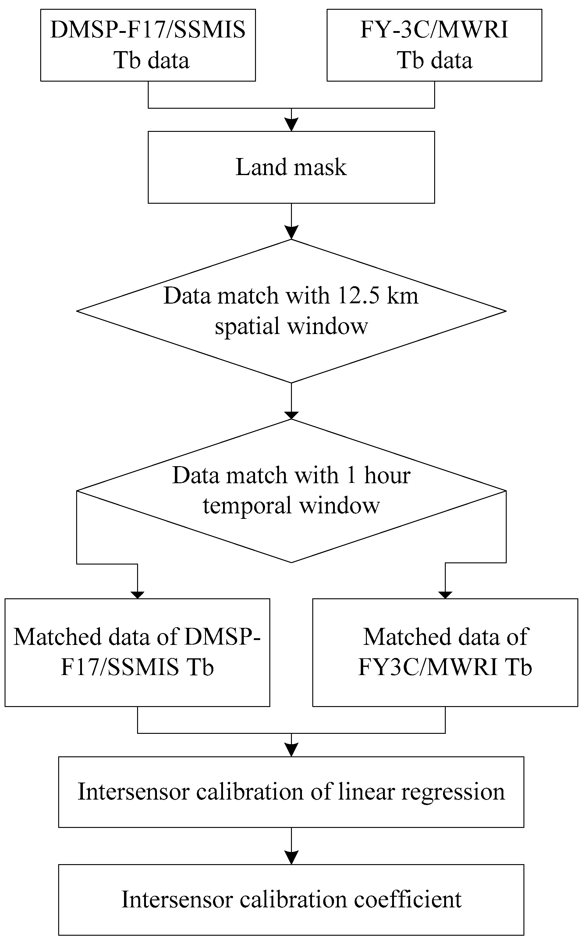
For intersensor calibrations between different satellites’ instruments, the first step is to find observations of the same ground object by two satellites in the same or a similar observation time. For the Tb data of the SSMIS and MWRI, each sampling point of each data swath provides the geographic location (latitude and longitude) and sampling time. According to the method of projection described in the previous subsection, each swath data point was projected at the North and South Poles with a spatial resolution of 12.5 km, and then the observations of land area were eliminated. Then, the data matchup was carried out with a spatial window of 12.5 km and a temporal window of 1 h. Based on the matched Tb data of each band, the corresponding linear regression coefficients were calculated. Figure 3 shows the flow chart of intersensor calibration.
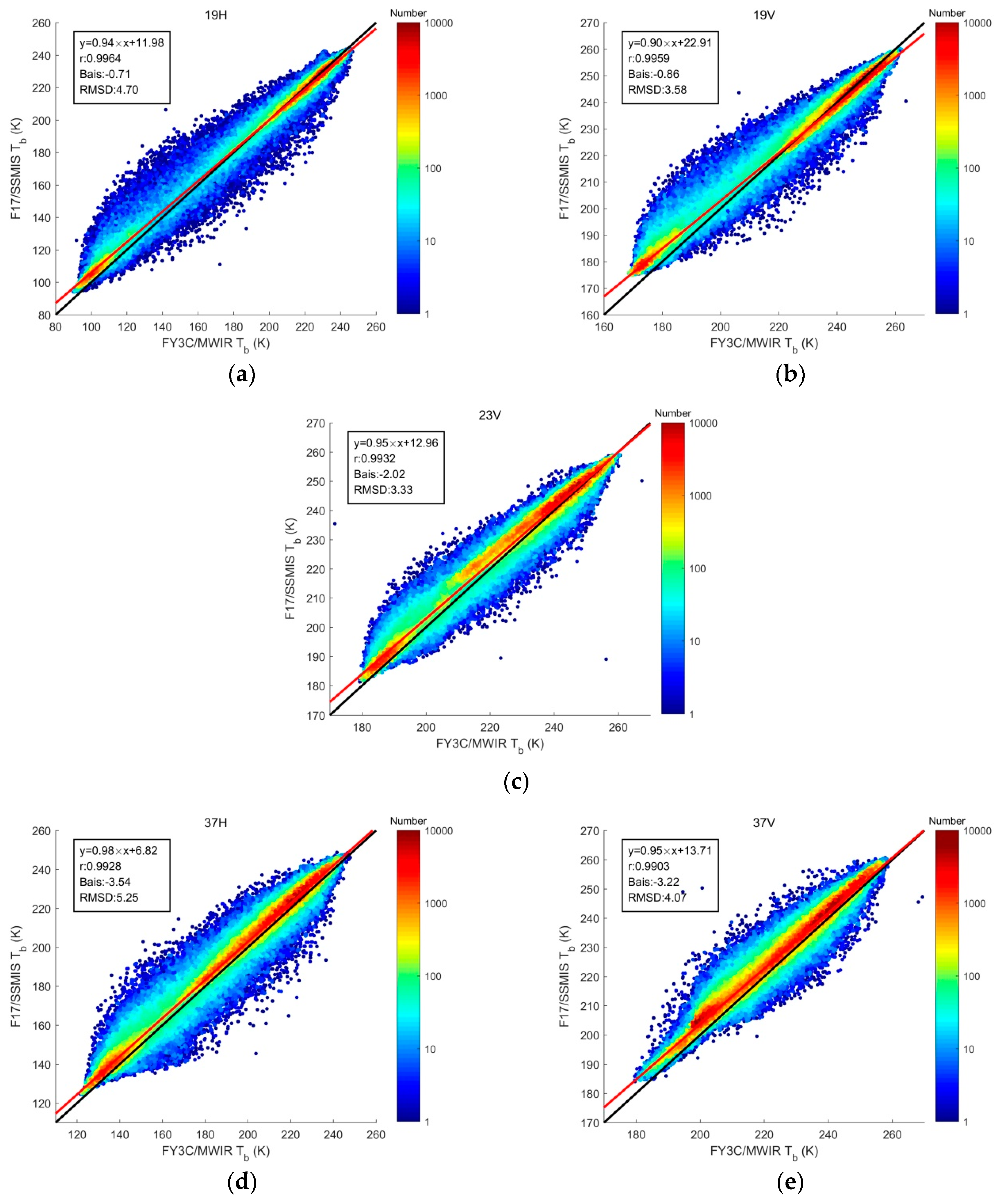
To calculate the calibration coefficient more accurately, we selected the matched data of the 1st, 11th, and 21st days of each month to obtain the calibration coefficients of 12 months. With the coefficients, the calibrated Tb data of MWRI were used to retrieve the SIC in the subsequent work. Figure 4 shows the scatter diagrams of matched data of 3 days in March 2016. In total, 565,114 pairs of Tbs for each channel were compared. The Tb of FY3C/MWIR is the abscissa, and the Tb of F17/SSMIS is the ordinate. To display the density distribution of matched data, the point numbers were calculated with the base 10 logarithm and displayed according to the color bar. The 1:1 line is shown with a black line, and the established intersensor calibration model is shown with a red line. The text box lists the detailed information, including the intersensor calibration formula, matched data’s correlation coefficient (r), bias, and root mean square deviation (RMSD).
Table 2 shows the 12-month calibration coefficients, where the values of SLOPE and OFFSET were used for intersensor calibration of the Tb data of MWRI with the following equation:
where FF is the frequency in GHz (e.g., 19, 23, and 37) and P is the polarization (v: vertical; h: horizontal).
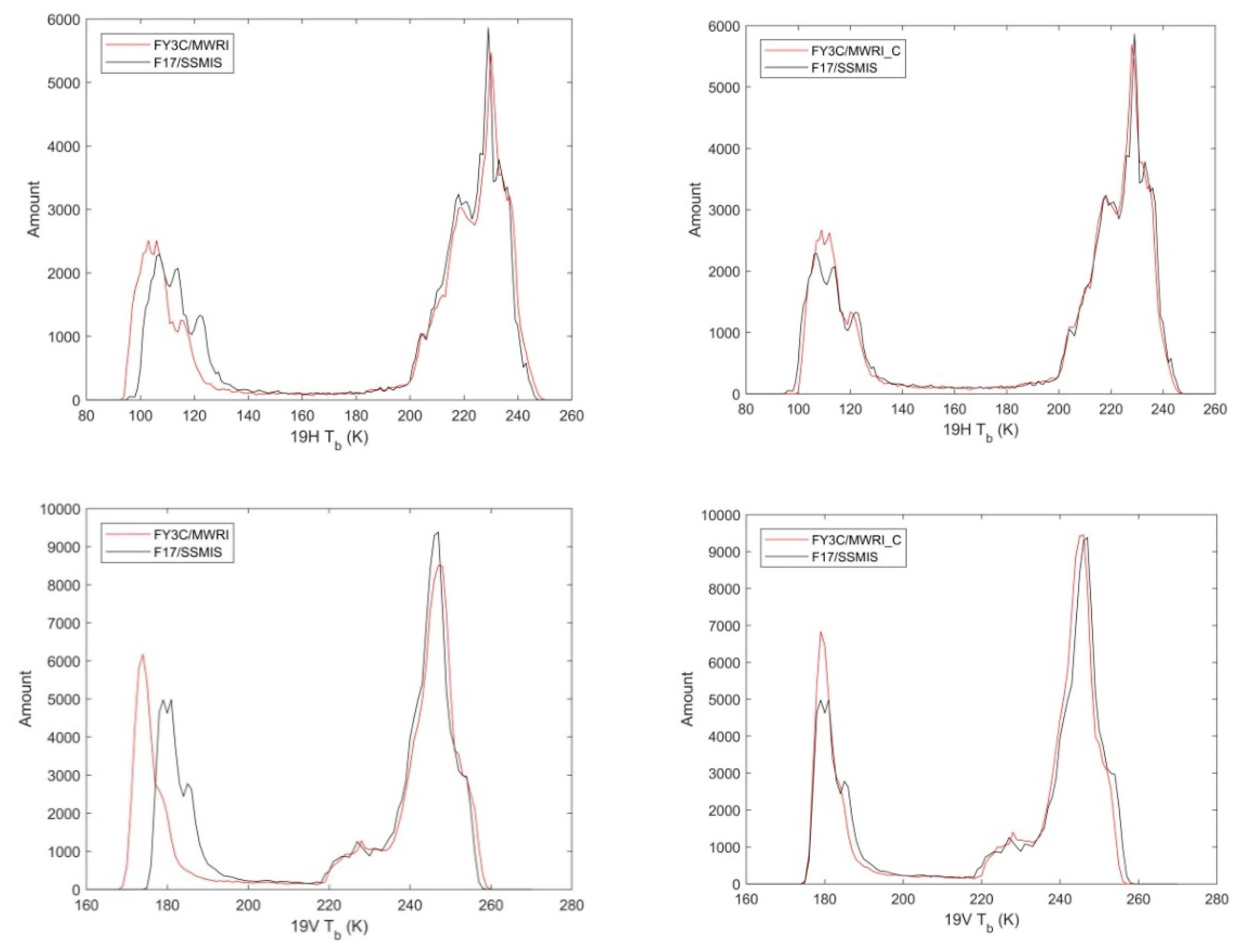
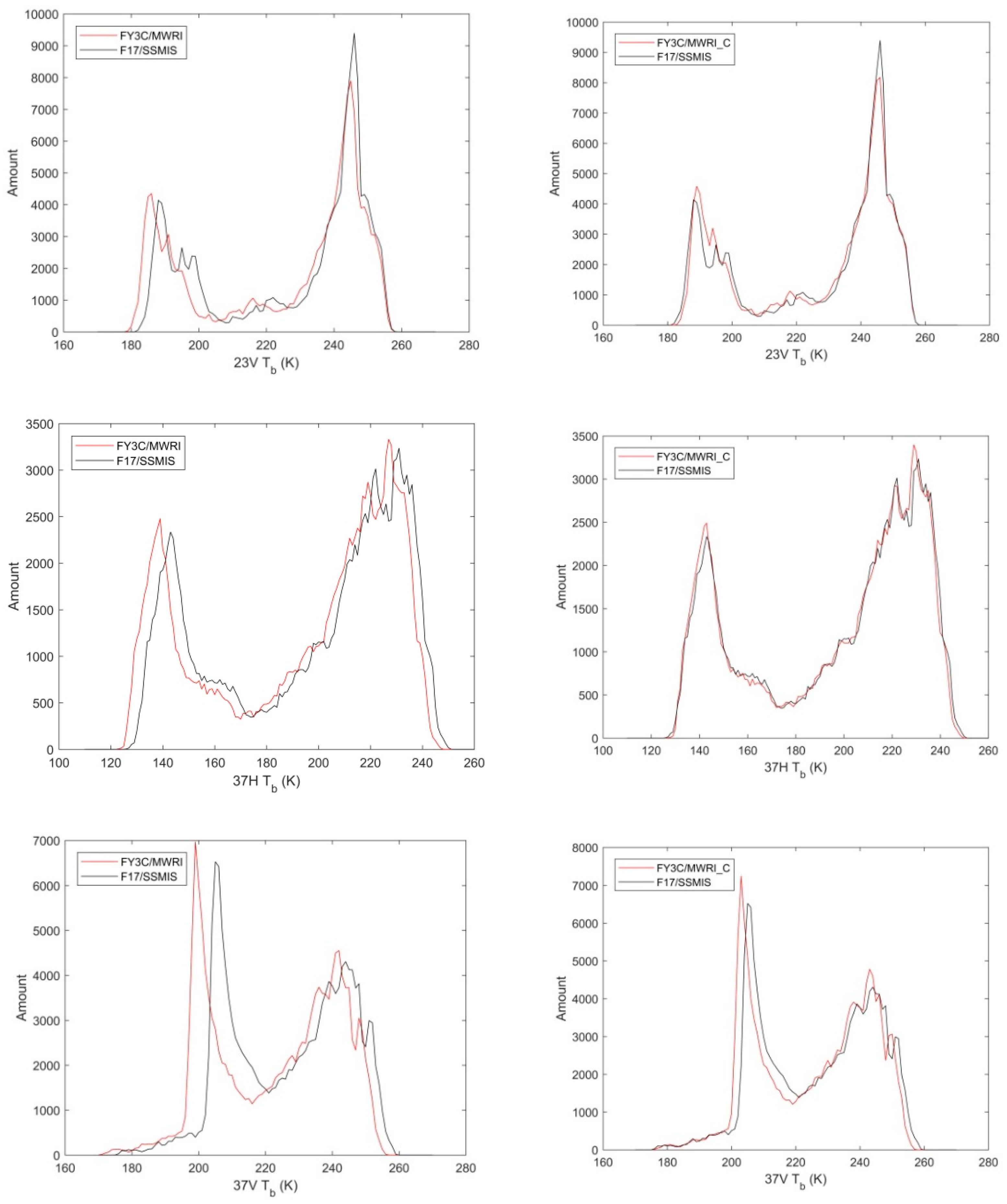
Based on Equation (1) and the intersensor calibration coefficients of Table 2, the Tb values at all channels of MWRI were calibrated. Figure 5 shows the histograms of the original and calibrated Tbs at all channels of F17/SSMIS, original FY3C/MWRI, and calibrated FY3C/MWRI on 1 March 2017. The Tb histograms depict the number of matched data pixels (amount) at each channel in steps of 1 K. After the calibration, the correlation coefficients between the histograms of F17/SSMIS and FY3C/MWRI at the 19H, 19V, 23V, 37H, and 37V channels have improved from 0.9399 to 0.9855, from 0.7788 to 0.9688, from 0.9091 to 0.9812, from 0.9097 to 0.9918, and from 0.5930 to 0.8552, respectively. The calibration effects of vertical polarization are better than those of horizontal polarization.
4. SIC Retrieval
Based on the NASA team method, SICs were retrieved with FTPs and DTPs. The retrieved SIC products are abbreviated as FY3C and FY3C_DTP. Then, the inversion results were processed further to remove the spurious ice over the open ocean caused by atmospheric effects and to decrease the overestimated SIC along the coastline caused by land contamination.
4.1. NASA Team Method with Fixed Tie Points Based on the Intersensor Calibrated Tb
With the calibrated and projected Tb of FY3C/MWRI, the SIC of the polar zone with 25 km spatial resolution was calculated based on the NT algorithm [25]. For the original NT algorithm, the tie points are a set of typical fixed Tb values of multiyear ice (MYI), first-year ice (FYI), and open water based on experimental and statistical studies [26]. In this study, the tie points of the F17/SSMIS version of the NASA team SIC algorithm were used to retrieve the SIC. The thresholds of two weather filters [26] use the values of the F17/SSMIS version. If the spectral gradient ratios GR(37/19) and GR(22/19) are larger than the thresholds, the SIC is set to zero. With these filters, the spurious ice over the open ocean caused by the presence of atmospheric water vapor, cloud liquid water, and precipitation can be decreased effectively. Table 3 lists the values of the tie points and thresholds of the two weather filters [27].
4.2. NASA Team Method with Dynamic Tie Points Based on the Original Tb
For the NT method, the tie points are unique sets for each hemisphere and each sensor used in the data product. However, these tie points, representing the typical Tb of multiyear ice, FYI and OW, have seasonal and annual variations and have a range of variability for the same ice type of OW due to atmospheric conditions and surface temperature [28,29]. The FTPs will introduce errors in the estimation of SIC. Therefore, the DTPs should be more reasonable for SIC retrieval [30]. For the MYI and FYI, the daily tie point values are the mean Tb values of all data points with greater than 95% MYI and FYI SIC products, respectively, described in Section 4.1. For ocean water, the daily tie point values are the mean Tb values over the regions with 0% SIC of Section 4.1 and with GR(37/19) and GR(22/19) values smaller than the thresholds shown in Table 3. A 2-pixel extended land mask was used to exclude the coastal zone from OW. Then, the daily tie points were filtered with a [−7; +7 days] sliding window [29] and used for SIC retrieval.
4.3. Land Contamination Effect Remove
Due to the coarse spatial resolution of microwave radiometers, the blurring of sharp contrasts in Tb between land and ocean results in false SICs along the coastlines, which is called land-to-ocean spillover effect or land contamination. This effect can be removed with the method described by Parkinson et al. (1987) [6]. This method assumes that the minimum observed SIC along the coastline in summer is the result of land spillover. Therefore, the false sea ice near the coastline is subtracted from the preliminary result of daily inversion of SIC to remove the land contamination effect.
For residual weather pollution and land contamination that cannot be removed by weather filters, sea ice masks are removed. For the Arctic, the valid ice mask derived from National Ice Center monthly sea ice climatology is used. For the Antarctic, the sea ice mask uses the data with the largest sea ice range in September and expands the maximum sea ice range by four more grids.
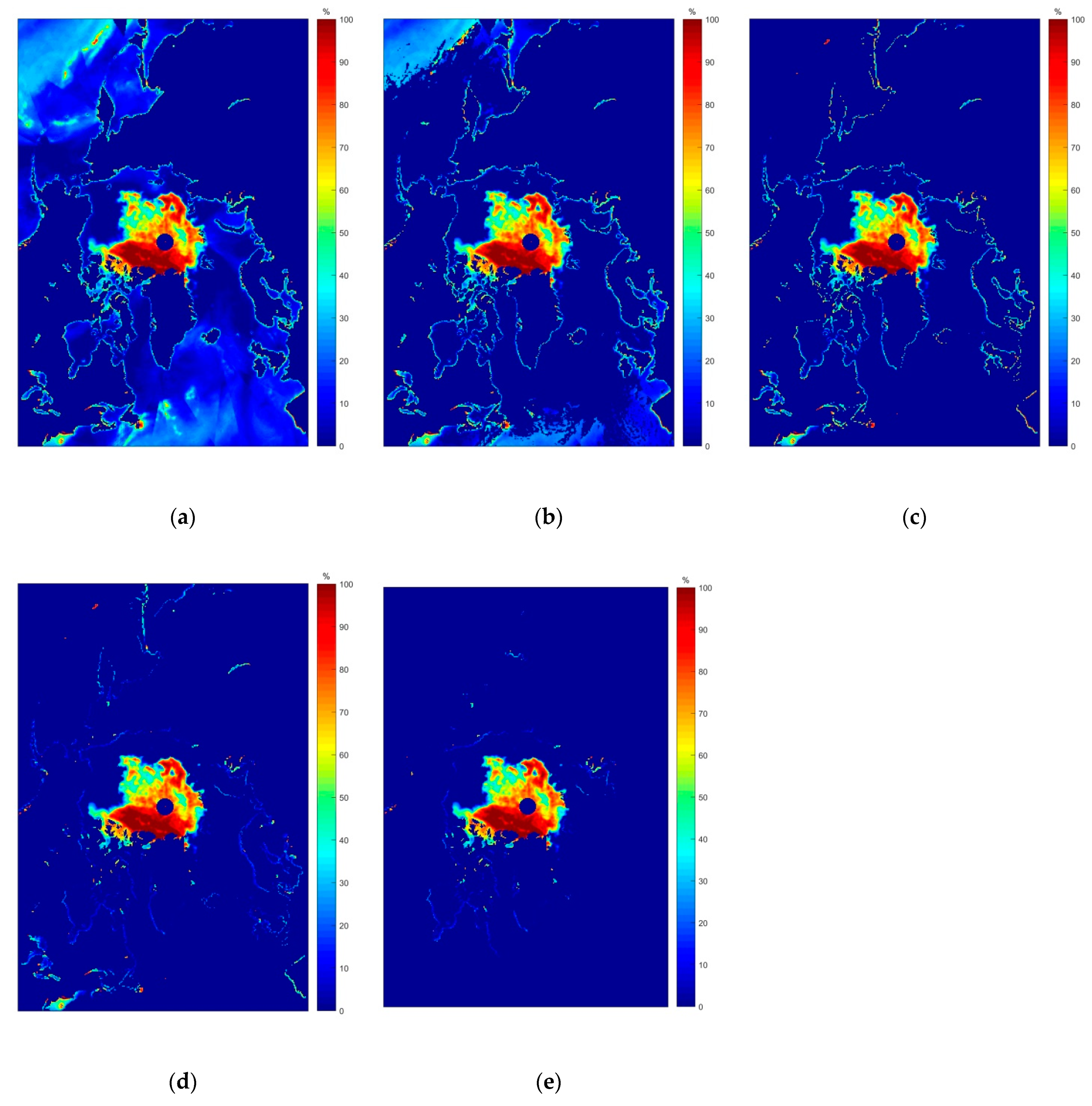
Figure 6 shows the step-by-step correction results from the preliminary results of the retrieved SIC to the final results using the Tb data of 26 August 2017. Figure 6a shows the preliminary result of inversion. The weather over the open sea area is severely affected (10–15 m/s wind speed and 2 mm/h rainfall rate [31]), and there is much false sea ice. Figure 6b shows the result with the GR(37/19) weather filter, which effectively removes the false sea ice caused by liquid water (0.1–0.3 mm [31]) over the high-latitude area. However, there are still incorrect results in the middle latitudes, which are caused by higher atmospheric water vapor (30–45 mm [31]). Figure 6c shows that most false sea ice caused by weather effects can be removed with further processing with GR(22/19). Figure 6d shows the result with the land contamination correction method of Parkinson et al. (1987) [6]. By comparing Figure 6c and 6d, it can be seen that there are obvious land pollution phenomena at land–sea junctions (such as the Kamchatka Peninsula, Alaska Peninsula, Scandinavia Peninsula, and Great Britain Island), misevaluating a large amount of false sea ice. The land spillover effect has been corrected effectively. Finally, the valid ice mask was used to remove residual weather pollution and land contamination, and the result is shown in Figure 6e.
5. Intersensor Comparison in the SIC
To compare the obtained SIC data of FY3C, FY3C_DTP, and NSIDC, the SIEs over the Arctic and Antarctic from the different SIC data were calculated. The SIE is defined as the sum of the area of all grids with an SIC of 15% or greater. Each grid is nominally 625 km2, but the actual area represented by each grid is different due to the polar stereographic projection. Therefore, the area of each grid is given by the static reference files from the NSIDC. The SIC near the North Pole not observed by the microwave radiometer is assumed to be greater than 15%, so the Arctic Pole Hole area is included in the SIE of the Arctic.
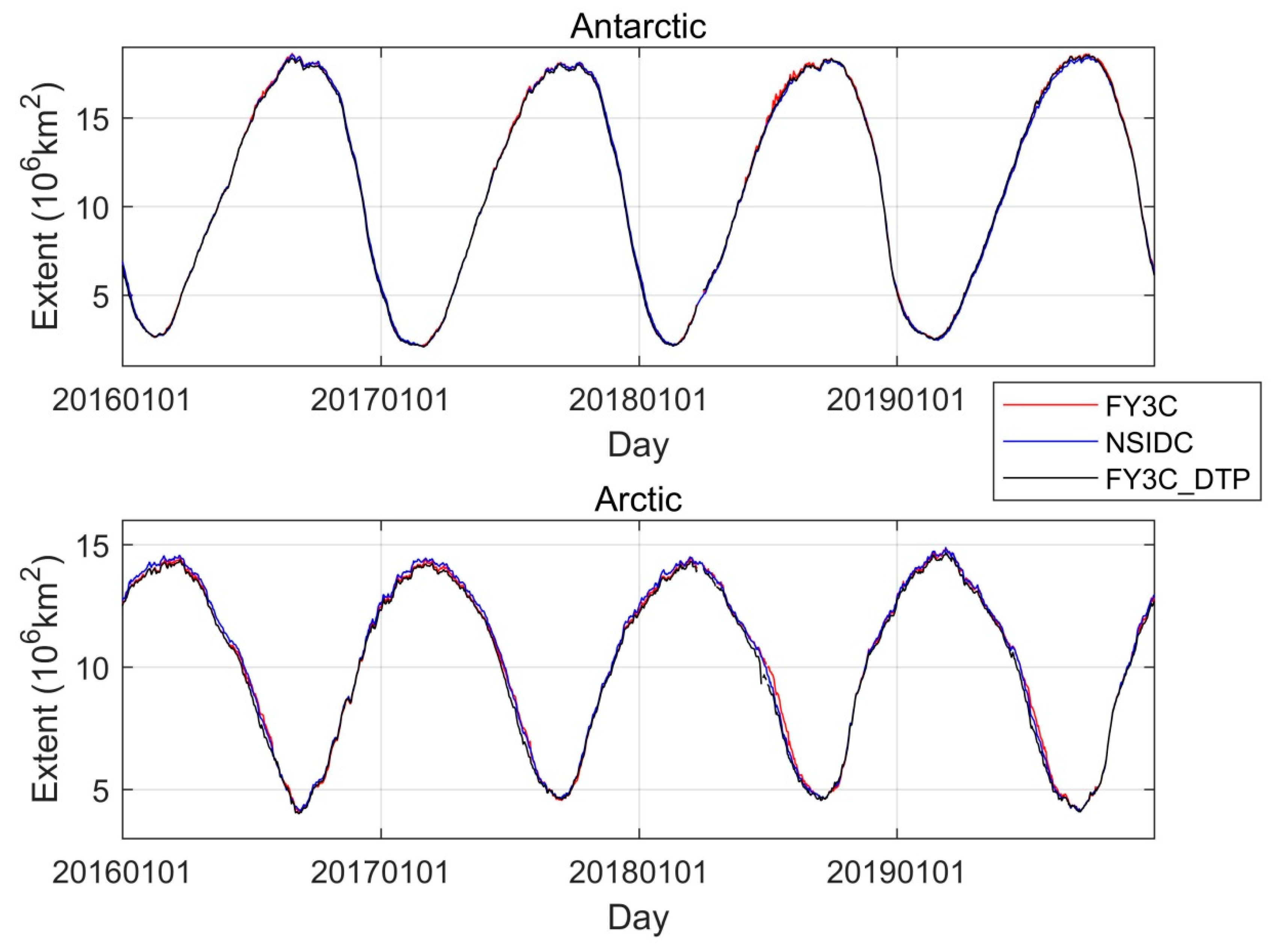
Figure 7 shows the daily SIE over 4 years (2016–2019) over the Arctic and Antarctic with different SIC data. The SIE time series of the three datasets are very close and show the same seasonal changes. For the Antarctic, the SIE of FY3C in the summers of 2018 and 2019 is higher than that of NSIDC and the SIE of FY3C_DTP is between that of FY3C and NSIDC. For the Arctic, the SIE of FY3C in winter is lower than that of NSIDC, while the SIE of FY3C in summer of 2018 and 2019 is higher than that of NSIDC. The SIE of FY3C_DTP is the lowest among these three datasets.
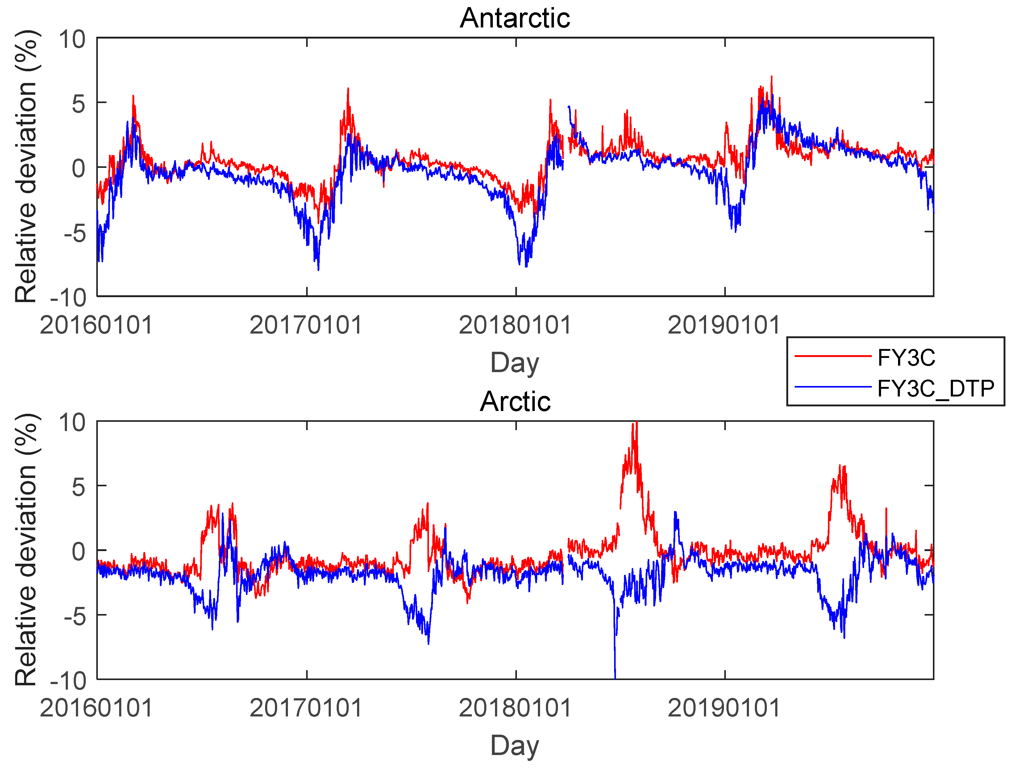
To further quantitatively evaluate the difference among these three datasets, the daily SIE difference percentage of FY3C vs. NSIDC and FY3C_DTP vs. NSIDC of 4 years over the Arctic and Antarctic was calculated and is shown in Figure 8. In 2016 and 2017, there is a negative deviation for FY3C vs. NSIDC from December to February of the next year and a positive deviation from March to April over the Antarctic. After 2018, the deviation becomes positive over the Antarctic. Over the Arctic, there is a positive deviation from July to September and a small negative deviation in other months. Table 4 shows the mean value and standard deviation of the relative deviation in Figure 7 for all four years and for each year. The average relative difference is 0.53 ± 1.50 for the Antarctic and –0.27 ± 1.85 for the Arctic, which is acceptable. However, the relative difference has a trend of increasing year by year, especially for the Antarctic, which can also be seen from Figure 8. For the Antarctic, the deviation of FY3C_DTP vs. NSIDC is larger than that of FY3C vs. NSIDC. For the Arctic, the deviation from July to September is negative because of the use the DTPs for SIC retrieval.
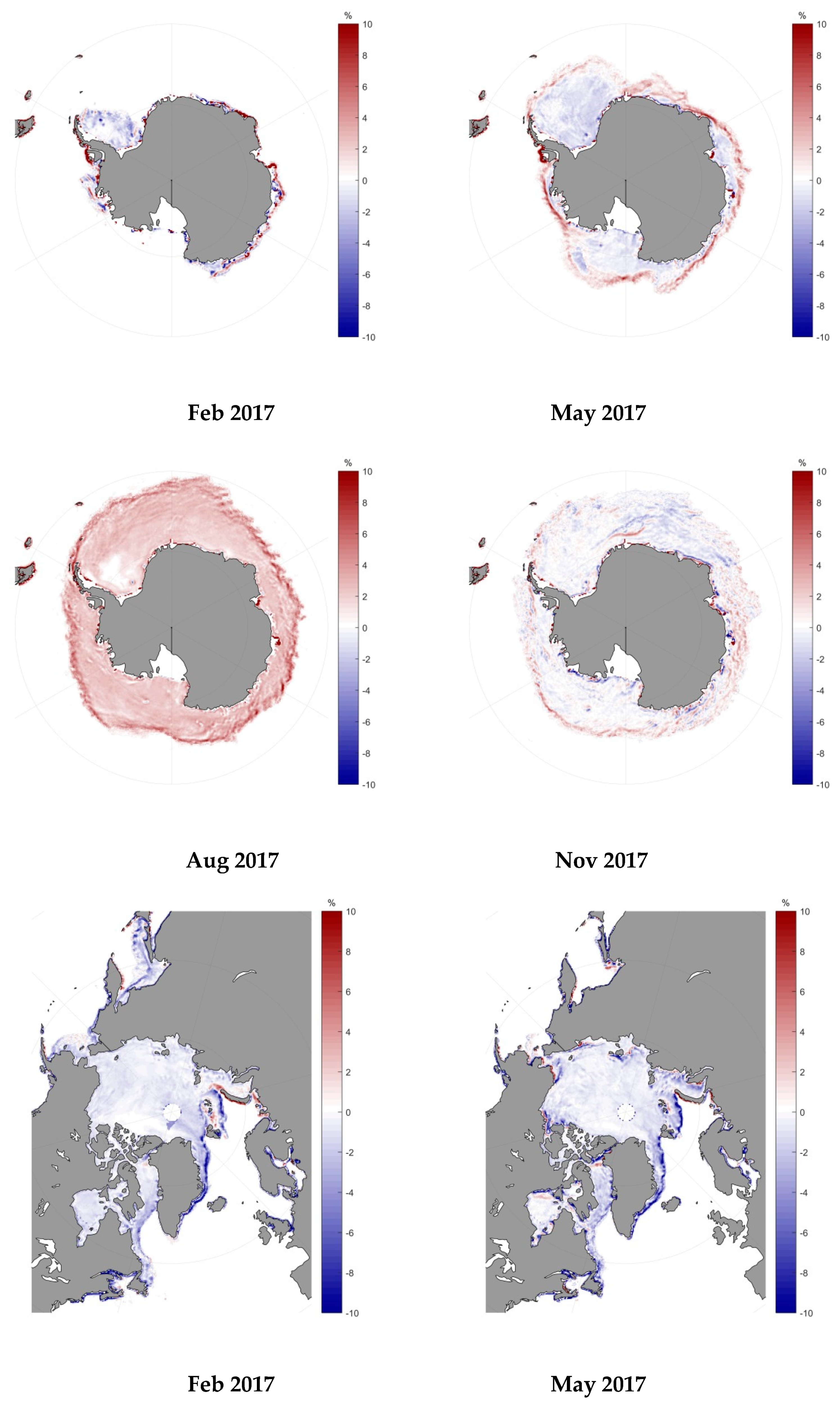
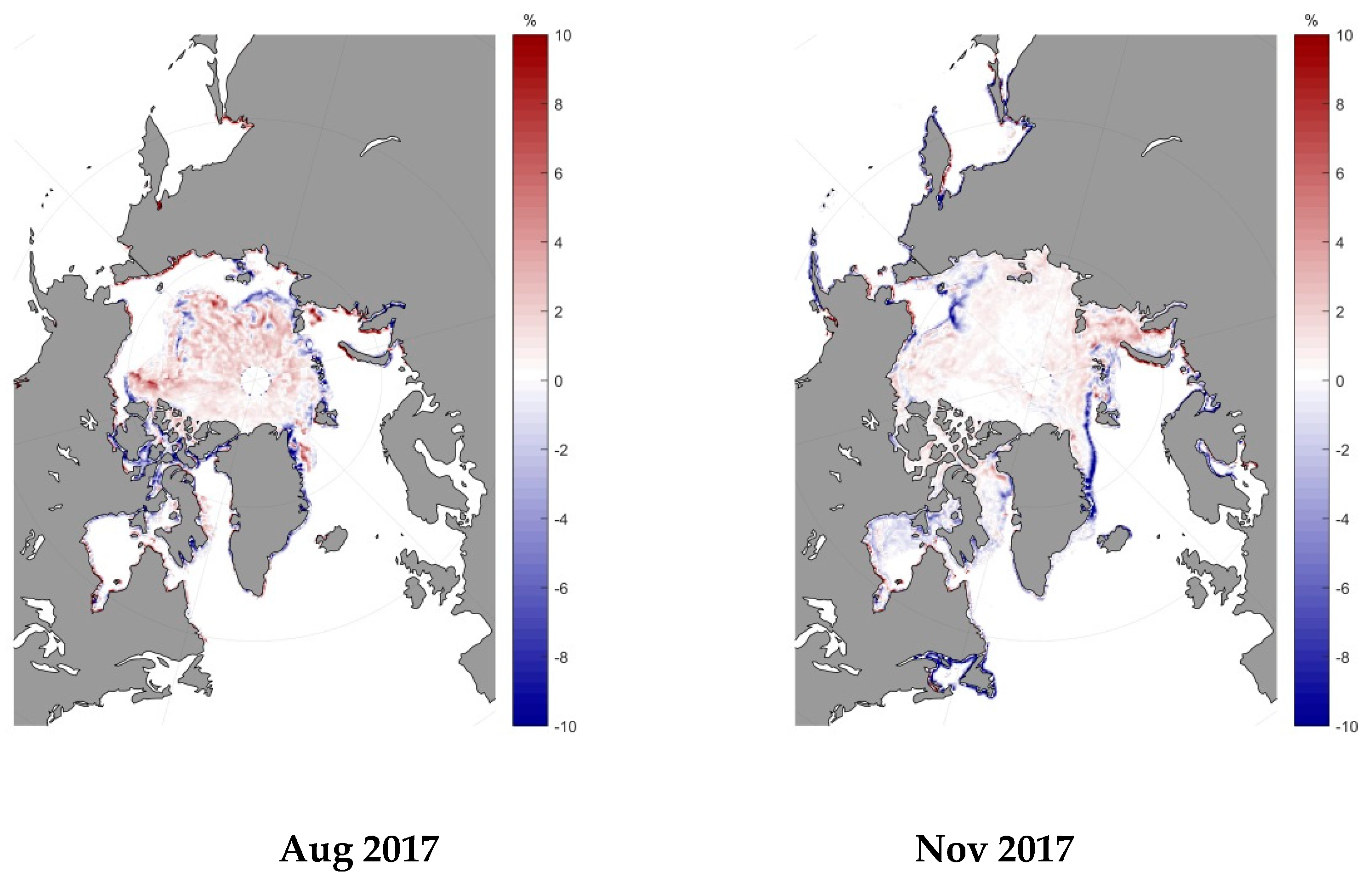
With the daily SIC difference between FY3C and NSIDC, the monthly averaged difference was calculated. Figure 9 shows the average difference in SIE in four typical months of 2017. The difference shown in red indicates that the result of FY3C is higher than that of NSIDC, and blue indicates that the result of FY3C is lower than that of NSIDC. For Antarctica, the SIE over the Weddell Sea is underestimated in February and overestimated over some marginal ice zones (MIZs); in May, the SIC over the MIZs is overestimated, and the values over other regions are slightly lower than the NSIDC result; in August, the result of FY3C is generally high; in November, the result over the MIZ of the Ross Sea is overestimated, and the differences in other sea areas are small. For the Arctic, the sea ice margin is underestimated in February and May; in August and November, except for the MIZ, the results of other regions are slightly higher than the NSIDC results.
6. Evaluation with Ancillary Data
6.1. Evaluation with OBS SIC Data
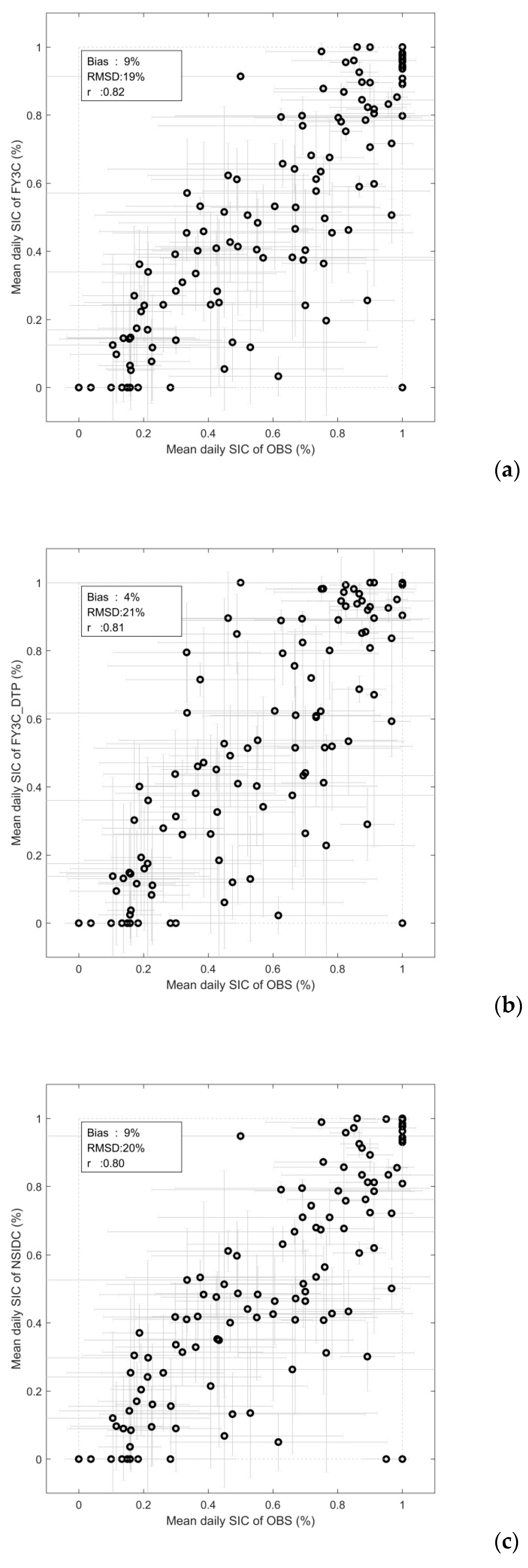
The temporal and spatial scales between OBS SIC and PM SIC are quite different. To reduce the subjectivity of visual observations, we first averaged the OBS SIC in each 25 × 25 km grid according to the spatial resolution (25 km) and location of the satellite PM SIC product, and then calculated the average OBS SIC and PM SIC along the ship track over one day. Finally, 95 pairs of matched data over the Arctic and 24 pairs over the Antarctic were obtained. The matched daily SIC values and their statistical analysis results are shown in Figure 10. The bias, RMSD, and correlation coefficient of the statistical analysis are also given in Figure 10. Compared with the OBS SIC data, the SIC results of FY3C and NSIDC are similar and underestimate the SIC with 9% bias. Even the results of FY3C are slightly better, the RMSD is 19% and the correlation coefficient is 0.82, better than 20% and 0.80, respectively, of NSIDC. Most OBS SIC data are from the sea ice melting season, i.e., from May to October for the Arctic and October to December for the Antarctic. This underestimation result of the NT method in summer is consistent with the results of Kern et al. (2019) and Alekseeva et al. (2019) [32,33]. The tie point values of the ice melting season change more dramatically than those of other periods. Using the dynamic tie points, the SIC bias of FY3C_DTP is 4%, which is better than that of the other two products. The smaller bias of FY3C_DTP proves that the dynamic tie points reflect the seasonal change of different sea ice types’ Tb and improve the accuracy of SIC.
6.2. Evaluation with SAR Data
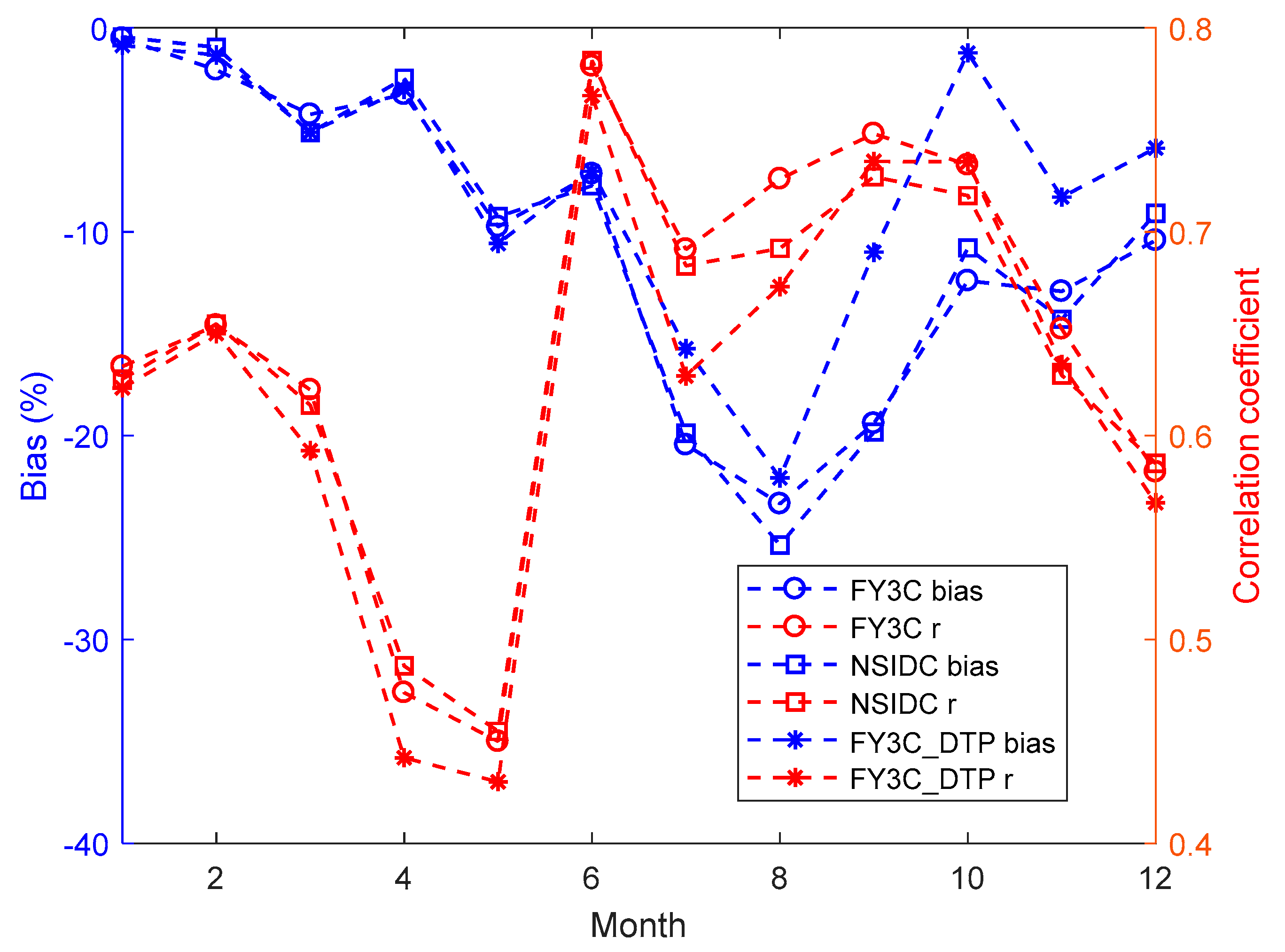
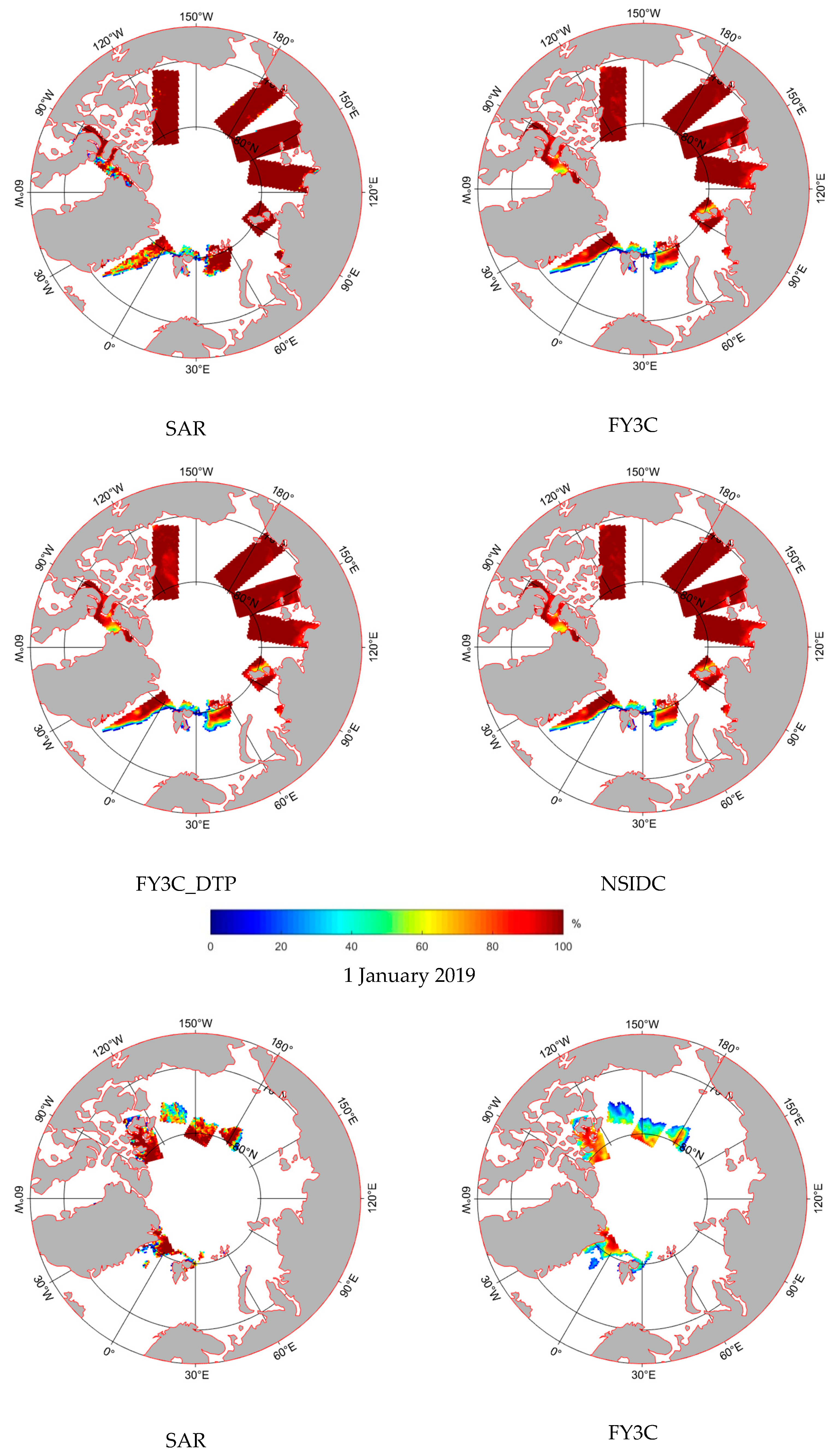
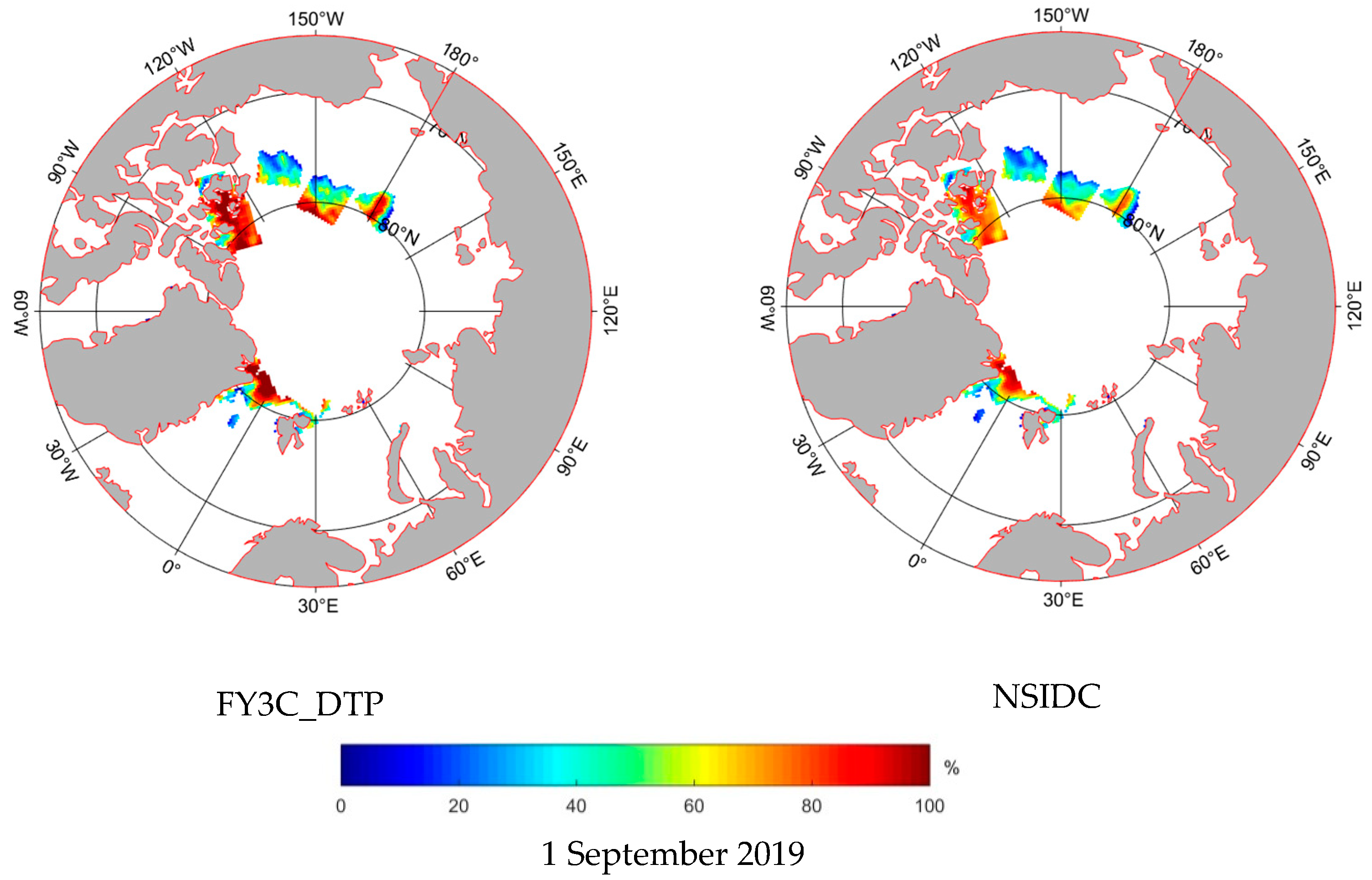
Based on the sea ice cover results of S1 SAR with a spatial resolution of 400 m and the polar stereographic projection, the number of sea ice covered pixels in each 25 × 25 km grid was counted, and then the SIC data with a 25 km spatial resolution was obtained by dividing the total number of pixels. To decrease the land spillover effect on SIC retrieval, the 25 × 25 km grid including land was excluded from the SIC results of S1 SAR. Figure 11 shows the daily bias and correlation coefficient of the matched data with SIC > 0%. The deviation is small and the correlation coefficient is high during the winter. For example, on 1 February, the deviations of FY3C, FY3C_DTP, and NSIDC are −0.51%, −0.86%, and −0.44%, respectively, and the corresponding correlation coefficients are 0.63, 0.62, and 0.63. During the sea ice melting season, the deviation increases and the correlation coefficient decreases. For example, the biases of FY3C, FY3C_DTP, and NSIDC of 1 September are −19.39%, −11.00, and −19.82%, respectively, and the corresponding correlation coefficients are 0.75, 0.73, and 0.73, respectively. Figure 12 shows the SIC distribution of SAR, FY3C, FY3C_DTP, and NSIDC on1 January and 1 September 2019. The main difference on 1 January is over the sea ice edge area on the east and west sides of Iceland, and the SIC results of FY3C and NSIDC are obviously underestimated compared with the SAR results. In addition to the sea ice edge area, the main difference on 1 September also includes the MYI area near Canadian Arctic Archipelago and Greenland. The SIC results of FY3C and NSIDC are also underestimated, which is mainly caused by the changes in sea ice Tb caused by the rise in temperature, the melting of snow on the surface of the sea ice, and the generation of melt pond. From the SIC result of FY3C_DTP, the abovementioned underestimation can be partly resolved using dynamic tie points.
6.3. Evaluation with RRDP Data
With the OW and CI data of the RRDP dataset, the uncertainties for FY3C and FY3C_DTP of 2016 were evaluated. For the final SIC products, SICs were truncated at 0% and 100%, i.e., SIC values < 0% were set to 0% and SIC values > 100% were set to 100%. Table 5 shows the mean value and standard deviation for CI, SIC = 100%. Here, we evaluated the truncated SIC and nontruncated SIC of FY3C and FY3C_DTP [32]. For nontruncated results, FY3C underestimates SIC and FY3C_DTP overestimates SIC. The bias of the Antarctic is larger than that of the Arctic, and the standard deviation (SD) of the Antarctic is smaller than that of the Arctic. Using the dynamic tie point, the bias and SD of FY3C_DTP are smaller than those of FY3C. The bias of the Antarctic is reduced by ~4% (from 8.95% to 4.57%), and the SD is reduced by ~1%. The bias of the Arctic is reduced by ~2% (from 3.36% to 1.54%), and the SD is reduced by ~1%. For the truncated results, FY3C and FY3C_DTP underestimate SIC because all SIC values larger than 100% are set to 100%.
For OW, SIC = 0% (Table 6), the FY3C_DTP results of Antarctic summer and Arctic winter are not improved by using the DTPs, e.g., the bias increases by ~2% in Antarctic summer and by ~1% in Arctic winter. However, the results of Antarctic winter and Arctic summer are improved, the bias of Antarctic winter is reduced by ~1%, and the bias of Arctic summer is reduced by ~2%.
7. Data Availability
The SIC dataset of the FY3C MWRI over the Antarctic and Arctic in 2016–2019 is available at http://0-www-dx-doi-org.brum.beds.ac.uk/10.11922/sciencedb.00511; accessed on 6 January 2021 (Shi, 2021) [34]. In the ZIP file, the daily SIC data are provided in HDF format and named by FY3C_MWRI_YYYYMMDD_n(s).H5, where FY3C is the satellite name, MWRI is the sensor’s name, YYYYMMDD is the year, month, and day, and n (s) is Arctic (Antarctic). SIC is stored as a floating-point number in each record.
8. Conclusions
The consistency of long time series geophysical observation data is very important for climate research. Based on the Tb of the FY3C MWRI, the SIC was retrieved with the FTPs NT method and DTPs NT method. The main conclusions are as follows:
- (1)
- First, an intersensor calibration model was established based on the bright temperature data of each channel of the F17 SSMIS and FY3C MWRI in 2016. After the calibration, the correlation coefficients between the amounts of F17/SSMIS and FY3C/MWRI at the 19H, 19V, 23V, 37H, and 37V channels improved from 0.9399 to 0.9855, from 0.7788 to 0.9688, from 0.9091 to 0.9812, from 0.9097 to 0.9918, and from 0.5930 to 0.8552, respectively. Then, the weather filters with GR(37/19) and GR(22/19) were used to reduce the spurious ice result over the open water area with high atmospheric water vapor and cloud liquid water; the land contamination correction method was used to remove false sea ice over coastal area caused by land spillover effects; the residual weather pollution and land contamination were removed with the valid ice masks. All these processing steps were necessary and effective to remove the spurious ice over the open ocean and coastal zone.
- (2)
- With the FTPs NT method and intersensor calibrated Tb of the FY3C MWRI, the SIC products over the Antarctic and Arctic in 2016–2019 were retrieved and compared with the SIC data of the NSIDC. The average relative difference of the Arctic and Antarctic is acceptable, at −0.27 ± 1.85 and 0.53 ± 1.50, respectively. However, there are still some differences over the MIZ. FY3C MWRI is an alternative data source for polar sea ice observations.
- (3)
- The SIC products with the FTPs NT method and DTPs NT method were evaluated with ship observation data, SAR SIE data and RRDP data. In comparison with the ship observation data, the SIC bias of FY3C with DTP is 4% and is much smaller than that of FY3C with FTP (9%). Evaluation results with S1 SAR SIC data of 2019 show the SIC bias with DTP is smaller than that with FTP, especially for the latter half of the year. Evaluation with the CI data of the RRDP dataset shows a similar trend between FY3C SIC with FTPs and FY3C SIC with DTPs: the bias of the Antarctic is reduced by ~4% (from 8.95% to 4.57%), and the SD is reduced by ~1%; the bias of the Arctic is reduced by ~2% (from 3.36% to 1.54%), and the SD is reduced by ~1%. All the evaluation results show that the accuracy of SIC is improved by using DTPs. Compared with the FTPs, DTPs reflect the Tb seasonal changes in FYI and MYI, and the SIC retrieval errors are decreased.
In summary, this study lays a foundation for the release of operational SIC products with Chinese FY3C satellites. Future works will focus on a suitable SIC retrieval method for FY3C MWRI to improve the SIC accuracy.
Author Contributions
Data curation, L.S. and L.S.; writing, L.S.; methodology, L.S., S.L. and Y.S.; validation, X.A.; supervision and funding acquisition, B.Z. and Q.W. All authors have read and agreed to the published version of the manuscript.
Funding
This research was funded by National Key Research and Development Program of China grant number 2018YFC1407200 and IRASCC2020-2022-No.01-01-03.
Institutional Review Board Statement
Not applicable.
Informed Consent Statement
Not applicable.
Data Availability Statement
The data presented in this study are available on request from the corresponding author.
Acknowledgments
This work was partly supported by the National Key Research and Development Program of China (2018YFC1407200) and IRASCC2020-2022-No.01-01-03. The FY3C/MWRI Tb data were downloaded from the FENGYUN Satellite Data Center (http://satellite.nsmc.org.cn/, accessed on 28 April 2021). The authors would like to thank the National Satellite Meteorological Center (NSMC) for providing the FY3C data to users worldwide. The ancillary data, including SIC data of NSIDC (https://nsidc.org/, accessed on 28 April 2021), OBS data (https://www.pangaea.de/); accessed on 18 November 2020, and sea ice cover data of S1 SAR (http://0-www-dx-doi-org.brum.beds.ac.uk/10.11922/sciencedb.00273); accessed on 5 November 2020, are also acknowledged.
Conflicts of Interest
The authors declare no conflict of interest.
References
- Cheung, H.H.; Keenlyside, N.; Omrani, N.E.; Zhou, W. Remarkable link between projected uncertainties of Arctic sea-ice decline and winter Eurasian climate. Adv. Atmos. Sci. 2018, 35, 38–51. [Google Scholar] [CrossRef]
- Meier, W.N.; Hovelsrud, G.K.; Van Oort, B.E.; Key, J.R.; Kovacs, K.M.; Michel, C.; Haas, C.; Granskog, M.A.; Gerland, S.; Perovich, D.K.; et al. Arctic sea ice in transformation: A review of recent observed changes and impacts on biology and human activity. Rev. Geophys. 2014, 52, 185–217. [Google Scholar] [CrossRef]
- Kwok, R. Arctic sea ice thickness, volume, and multiyear ice coverage: Losses and coupled variability (1958–2018). Environ. Res. Lett. 2018, 13, 105005. [Google Scholar] [CrossRef]
- Curry, J.A.; Schramm, J.L.; Ebert, E.E. Sea ice-albedo climate feedback mechanism. J. Clim. 1995, 8, 240–247. [Google Scholar] [CrossRef]
- Perovich, D.; Richter-Menge, J.; Polashenski, C.; Elder, B.; Arbetter, T.; Brennick, O. Sea ice mass balance observations from the North Pole Environmental Observatory. Geophys. Res. Lett. 2014, 41, 2019–2025. [Google Scholar] [CrossRef]
- Parkinson, C.L. Arctic Sea Ice, 1973–1976: Satellite Passive-Microwave Observations; Scientific and Technical Information Branch, NASA: Washington, DC, USA, 1987.
- Titchner, H.A.; Rayner, N.A. The Met Office Hadley Centre sea ice and sea surface temperature data set, version 2: 1. Sea ice concentrations. J. Geophys. Res. 2014, 119, 2864–2889. [Google Scholar] [CrossRef]
- Witze, A. Ageing satellites put crucial sea-ice climate record at risk. Nature News 2017, 551, 13. [Google Scholar] [CrossRef] [PubMed] [Green Version]
- Available online: http://www.nsmc.org.cn/en/NSMC/Channels/FY_3C.html (accessed on 20 September 2019).
- FY3C-MWRI. Available online: http://satellite.nsmc.org.cn/PortalSite/StaticContent/DeviceIntro_FY3_MWRI.aspx (accessed on 23 March 2018).
- Available online: http://satellite.nsmc.org.cn/portalsite/default.aspx (accessed on 20 September 2019).
- Available online: https://www.star.nesdis.noaa.gov/mirs/ssmis.php (accessed on 20 September 2019).
- Remote Sensing Systems. Available online: http://www.remss.com/measurements/brightness-temperature/ (accessed on 10 April 2018).
- Hilburn, K.A.; Wentz, F.J. Intercalibrated Passive Microwave Rain Products from the Unified Microwave Ocean Retrieval Algorithm (UMORA). J. Appl. Meteorol. Climatol. 2008, 47, 778–794. [Google Scholar] [CrossRef] [Green Version]
- Frederick Pearson, I. Map Projections: Theory and Applications; CRC Press: Boca Raton, FL, USA, 1990. [Google Scholar]
- Snyder, J.P. Map Projections-A Working Manual; US Government Printing Office: Washington, DC, USA, 1987; Volume 1395.
- Cavalieri, D.J.; Parkinson, C.L.; Gloersen, P.; Zwally, H.J. Updated Yearly. Sea Ice Concentrations from Nimbus-7 SMMR and DMSP SSM/I-SSMIS Passive Microwave Data; Version 1; NASA National Snow and Ice Data Center Distributed Active Archive Center: Boulder, CO, USA, 1996. [CrossRef]
- Available online: https://www.pangaea.de/ (accessed on 18 November 2020).
- Worby, A.P.; Allison, I.A. Ship-Based Technique for Observing Antarctic Sea Ice: Part I: Observational Techniques and Results; Research Report No. 14; Antarctic Cooperative Research Centre: Hobart, Australia, 1999; Volume 14, 64p. [Google Scholar]
- Wang, Y.-R.; Li, X.-M. Arctic sea ice cover data from spaceborne SAR by deep learning. Earth Syst. Sci. Data Discuss. 2020, 1–30. [Google Scholar] [CrossRef]
- Wang, Y.-R.; Li, X.-M. Arctic Sea Ice Cover Product Based on Spaceborne Synthetic Aperture Radar. V1. Science Data Bank. Available online: http://0-www-dx-doi-org.brum.beds.ac.uk/10.11922/sciencedb.00273 (accessed on 5 November 2020).
- Pedersen, L.T.; Saldo, R.; Ivanova, N.; Kern, S.; Heygster, G.; Tonboe, R.T.; Huntemann, M.; Ozsoy, B.; Girard-Ardhuin, F.; Kaleschke, L. Reference Dataset for Sea Ice Concentration. 2019. Available online: https://0-doi-org.brum.beds.ac.uk/10.6084/m9.figshare.6626549.v6 (accessed on 18 March 2021).
- Lavergne, T.; Sørensen, A.M.; Kern, S.; Tonboe, R.; Notz, D.; Aaboe, S.; Bell, L.; Dybkjær, G.; Eastwood, S.; Gabarro, C.; et al. Version 2 of the EUMETSAT OSI SAF and ESA CCI sea-ice concentration climate data records. Cryosphere 2019, 13, 49–78. [Google Scholar] [CrossRef] [Green Version]
- Dai, L.; Che, T.; Ding, Y. Inter-Calibrating SMMR, SSM/I and SSMI/S Data to Improve the Consistency of Snow-Depth Products in China. Remote Sens. 2015, 7, 7212–7230. [Google Scholar] [CrossRef] [Green Version]
- Cavalieri, D.J.; Gloersen, P.; Campbell, W.J. Determination of sea ice parameters with the nimbus 7 SMMR. J. Geophys. Res. Atmos. 1984, 89, 5355–5369. [Google Scholar] [CrossRef]
- Cavalieri, D.J.; Parkinson, C.L.; DiGirolamo, N.; Ivanoff, A. Intersensor Calibration between F13 SSMI and F17 SSMIS for Global Sea Ice Data Records. IEEE Geosci. Remote Sens. Lett. 2012, 9, 233–236. [Google Scholar] [CrossRef] [Green Version]
- Cavalieri, D.J.; St Germain, K.M.; Swift, C.T. Reduction of weather effects in the calculation of sea ice concentration with the DMSP SSM/I. J. Glaciol. 1995, 41, 455–464. [Google Scholar] [CrossRef] [Green Version]
- Ivanova, N.; Pedersen, L.T.; Tonboe, R.; Kern, S.; Heygster, G.; Lavergne, T.; Sorensen, A.C.; Saldo, R.; Dybkjaer, G.; Brucker, L.; et al. Inter-comparison and evaluation of sea ice algorithms: Towards further identification of challenges and optimal approach using passive microwave observations. Cryosphere 2015, 9, 1797–1817. [Google Scholar] [CrossRef] [Green Version]
- Tonboe, R.T.; Eastwood, S.; Lavergne, T.; Sørensen, A.M.; Rathmann, N.; Dybkjær, G.; Pedersen, L.T.; Høyer, J.L.; Kern, S. The EUMETSAT sea ice concentration climate data record. Cryosphere 2016, 10, 2275–2290. [Google Scholar] [CrossRef] [Green Version]
- Ye, Y.; Heygster, G. Arctic Multiyear Ice Concentration Retrieval from SSM/I Data Using the NASA Team Algorithm with Dynamic Tie Points. In Towards an Interdisciplinary Approach in Earth System Science; Lohmann, G., Meggers, H., Unnithan, V., Wolf-Gladrow, D., Notholt, J., Bracher, A., Eds.; Springer Earth System Sciences; Springer: Cham, Switzerland, 2015. [Google Scholar] [CrossRef]
- Remote Sensing Systems. Available online: http://images.remss.com/amsr/amsr2_data_daily.html#top (accessed on 19 November 2018).
- Kern, S.; Lavergne, T.; Notz, D.; Pedersen, L.T.; Tonboe, R.T.; Saldo, R.; Sørensen, A.M. Satellite passive microwave sea-ice concentration data set intercomparison: Closed ice and ship-based observations. Cryosphere 2019, 13, 3261–3307. [Google Scholar] [CrossRef] [Green Version]
- Alekseeva, T.; Tikhonov, V.; Frolov, S.; Repina, I.; Raev, M.; Sokolova, J.; Sharkov, E.; Afanasieva, E.; Serovetnikov, S. Comparison of Arctic Sea Ice Concentrations from the NASA Team, ASI, and VASIA2 Algorithms with Summer and Winter Ship Data. Remote Sens. 2019, 11, 2481. [Google Scholar] [CrossRef] [Green Version]
- Shi, L. Sea Ice Concentration Products over Polar Regions with FY-3C/MWRI Data (2016–2019). V1. Science Data Bank. Available online: http://0-www-dx-doi-org.brum.beds.ac.uk/10.11922/sciencedb.00511 (accessed on 6 January 2021).
Figure 1.
Tb of 18.7H (a,b) and observation times (c,d) of the Arctic (left column) and Antarctic (right column). Arctic images contain 448 × 304 pixels, and Antarctic images contain 332 × 316 pixels.
Figure 1.
Tb of 18.7H (a,b) and observation times (c,d) of the Arctic (left column) and Antarctic (right column). Arctic images contain 448 × 304 pixels, and Antarctic images contain 332 × 316 pixels.

Figure 2.
Spatial distribution of ship SIC observation data (red, 2016; blue, 2017; black, 2019; left, Arctic; right, Antarctic).
Figure 2.
Spatial distribution of ship SIC observation data (red, 2016; blue, 2017; black, 2019; left, Arctic; right, Antarctic).

Figure 3.
Flow chart of intersensor calibration.

Figure 4.
Scatter diagrams of matched Tb data from FY3C and F17 for various channels of 3 days of March 2016: (a) 19H, (b) 19V, (c) 23V, (d) 37H, and (e) 37V. The intersensor calibration formula, correlation coefficient (r), bias, and root mean square deviation (RMSD) are given in the top left of every image for the matched data.

Figure 5.
Histograms of F17/SSMIS, original FY3C/MWRI, and calibrated FY3C/MWRI Tb of 1 March 2017 for each channel (left column: F17/SSMIS and original FY3C/MWRI; right column: F17/SSMIS and calibrated FY3C/MWRI (FY3C/MWRI_C); 1st row, 19H; 2nd row, 19V; 3rd row, 23V; 4th row, 37H; 5th row, 37V).
Figure 5.
Histograms of F17/SSMIS, original FY3C/MWRI, and calibrated FY3C/MWRI Tb of 1 March 2017 for each channel (left column: F17/SSMIS and original FY3C/MWRI; right column: F17/SSMIS and calibrated FY3C/MWRI (FY3C/MWRI_C); 1st row, 19H; 2nd row, 19V; 3rd row, 23V; 4th row, 37H; 5th row, 37V).


Figure 6.
Step-by-step correction results from the preliminary results of retrieved SIC. (a) The preliminary result of SIC inversion; (b) the result with GR(37/19) weather filter to remove the false sea ice caused by liquid water (0.1–0.3 mm) over the high-latitude area; (c) most false sea ice caused by weather effects can be removed with further processing with GR(22/19); (d) the result with land contamination correction method; (e) the valid ice mask is used to remove the residual weather pollution and land contamination.

Figure 7.
Daily SIE of 4 years (2016–2019) over the Antarctic and Arctic with SIC data of FY3C (red), NSIDC (blue), and FY3C_DTP (black).
Figure 7.
Daily SIE of 4 years (2016–2019) over the Antarctic and Arctic with SIC data of FY3C (red), NSIDC (blue), and FY3C_DTP (black).

Figure 8.
Daily relative deviation of the SIE over the Antarctic and Arctic of FY3C vs. NSIDC and FY3C_DTP vs. NSIDC.
Figure 8.
Daily relative deviation of the SIE over the Antarctic and Arctic of FY3C vs. NSIDC and FY3C_DTP vs. NSIDC.

Figure 9.
Average difference in the SIE in four typical months of 2017.


Figure 10.
Daily averaged SIC from PM compared to OBS: (a) FY3C, (b) FY3C_DTP, and (c) NSIDC. Vertical and horizontal bars denote the standard deviation of these averaged SIC values for PM and OBS, respectively. The bias, the root mean square deviation (RMSD), and the correlation coefficient (r) are given in the top left of every image.

Figure 11.
Daily bias (blue dotted lines) and correlation coefficient (red solid lines) of the matched data.
Figure 11.
Daily bias (blue dotted lines) and correlation coefficient (red solid lines) of the matched data.

Figure 12.
SIC distribution of SAR, FY3C, FY3C_DTP, and NSIDC on 1 January 2019 and 1 September 2019.
Figure 12.
SIC distribution of SAR, FY3C, FY3C_DTP, and NSIDC on 1 January 2019 and 1 September 2019.


Table 1.
Parameter comparison of F17/SSMIS and FY3C/MWRI.
| Satellite | DMSP-F17 | FY3C |
|---|---|---|
| Sensor | SSMIS | MWRI |
| Orbit height (km) | 850 | 836 |
| Viewing angle (°) | 53.1 | 45 |
| AECT 1 | 5.31 p.m. | 1.40-2.00 p.m. |
| Channels used in this study: footprint (GHz: km × km) | 19.3: 70 × 45 22.2: 60 × 40 37.0: 38 × 30 | 18.7: 30 × 50 23.8: 27 × 45 36.5: 18 × 30 |
| Swath width (km) | 1700 | 1400 |
1 AECT: Ascending Equator crossing time (UTC).
Table 2.
Intersensor calibration coefficients of 12 months.
| SLOPE | ||||||||||||
|---|---|---|---|---|---|---|---|---|---|---|---|---|
| Month | 1 | 2 | 3 | 4 | 5 | 6 | 7 | 8 | 9 | 10 | 11 | 12 |
| 19V | 0.89 | 0.90 | 0.90 | 0.91 | 0.90 | 0.91 | 0.89 | 0.89 | 0.90 | 0.90 | 0.91 | 0.90 |
| 19H | 0.93 | 0.94 | 0.94 | 0.94 | 0.93 | 0.94 | 0.92 | 0.93 | 0.93 | 0.93 | 0.94 | 0.93 |
| 23V | 0.93 | 0.95 | 0.95 | 0.94 | 0.94 | 0.94 | 0.89 | 0.92 | 0.93 | 0.94 | 0.95 | 0.95 |
| 37V | 0.94 | 0.94 | 0.95 | 0.96 | 0.96 | 0.95 | 0.94 | 0.94 | 0.95 | 0.96 | 0.96 | 0.95 |
| 37H | 0.97 | 0.98 | 0.98 | 0.98 | 0.98 | 0.98 | 0.98 | 0.98 | 0.99 | 0.99 | 0.99 | 0.97 |
| OFFSET | ||||||||||||
| Month | 1 | 2 | 3 | 4 | 5 | 6 | 7 | 8 | 9 | 10 | 11 | 12 |
| 19V | 26.12 | 23.73 | 22.91 | 23.00 | 23.73 | 23.77 | 28.30 | 26.31 | 24.95 | 23.36 | 22.17 | 24.00 |
| 19H | 14.81 | 12.08 | 11.98 | 12.71 | 14.77 | 14.72 | 18.30 | 15.67 | 15.33 | 14.92 | 12.79 | 13.26 |
| 23V | 17.30 | 12.65 | 12.96 | 15.17 | 16.82 | 17.24 | 26.79 | 21.61 | 17.56 | 15.60 | 12.80 | 13.59 |
| 37V | 16.31 | 16.64 | 13.71 | 12.10 | 13.62 | 15.99 | 17.82 | 16.67 | 15.49 | 13.51 | 12.25 | 15.30 |
| 37H | 9.33 | 7.42 | 6.82 | 7.37 | 8.12 | 7.67 | 7.85 | 7.26 | 6.39 | 6.27 | 6.03 | 8.72 |
Table 3.
Values of tie points and thresholds of two weather filters.
| NH | Tie Point (K) | SH | Tie Point (K) |
|---|---|---|---|
| 19V OW | 184.9 | 19V OW | 184.9 |
| 19H OW | 113.4 | 19H OW | 113.4 |
| 37V OW | 207.1 | 37V OW | 207.1 |
| 19V FYI | 248.4 | 19V Ice Type A | 253.1 |
| 19H FYI | 232.0 | 19H Ice Type A | 237.8 |
| 37V FYI | 242.3 | 37V Ice Type A | 246.6 |
| 19V MYI | 220.7 | 19V Ice Type B | 244.0 |
| 19H MYI | 196.0 | 19H Ice Type B | 211.9 |
| 37V MYI | 188.5 | 37V Ice Type B | 212.6 |
| Threshold | Threshold | ||
| GR(37/19) | 0.05 | GR(37/19) | 0.053 |
| GR(22/19) | 0.045 | GR(22/19) | 0.045 |
Table 4.
Mean value and standard deviation of the relative deviation in Figure 8 for all 4 years and for single years.
Table 4.
Mean value and standard deviation of the relative deviation in Figure 8 for all 4 years and for single years.
| 2016–2019 | 2016 | 2017 | 2018 | 2019 | |
|---|---|---|---|---|---|
| Antarctic (FY3C) | 0.53 ± 1.50 | 0 ± 1.20 | –0.06 ± 1.50 | 0.68 ± 1.48 | 1.53 ± 1.22 |
| Antarctic (FY3C_DTP) | –1.86 ± 1.37 | –1.01 ± 1.62 | –1.07 ± 1.92 | –0.29 ± 2.34 | 1.00 ± 1.96 |
| Arctic (FY3C) | –0.27 ± 1.85 | –0.98 ± 1.40 | –1.00 ± 1.13 | 0.52 ± 2.39 | 0.39 ± 1.65 |
| Arctic (FY3C_DTP) | –0.34 ± 2.14 | –1.89 ± 1.28 | –2.20 ± 1.36 | –1.68 ± 1.35 | –1.67 ± 1.44 |
Table 5.
Comparison results to the 100% SIC dataset of RRDP for the Antarctic and Arctic. The results are given with bias ± standard deviation, and all values in these rows are given in percent SIC.
Table 5.
Comparison results to the 100% SIC dataset of RRDP for the Antarctic and Arctic. The results are given with bias ± standard deviation, and all values in these rows are given in percent SIC.
| Antarctic (4235) | Arctic (25865) | |||
|---|---|---|---|---|
| Nontruncated | Truncated | Nontruncated | Truncated | |
| FY3C | –8.95 ± 7.43 | –9.22 ± 6.00 | –3.36 ± 10.48 | –5.73 ± 8.23 |
| FY3C_DTP | 4.57 ± 6.57 | –1.15 ± 2.93 | 1.54 ± 9.61 | –2.86 ± 5.87 |
Table 6.
As in Table 5 but for SIC = 0%.
Table 6.
As in Table 5 but for SIC = 0%.
| Antarctic | Arctic | |||
|---|---|---|---|---|
| Summer (605) | Winter (366) | Summer (305) | Winter (300) | |
| FY3C | −1.23 ± 4.37 | 1.43 ± 4.76 | 2.53 ± 5.56 | −0.99 ± 4.96 |
| FY3C_DTP | −1.26 ± 6.52 | 0.22 ± 5.00 | 0.13 ± 6.79 | −1.60 ± 5.62 |
Publisher’s Note: MDPI stays neutral with regard to jurisdictional claims in published maps and institutional affiliations. |
© 2021 by the authors. Licensee MDPI, Basel, Switzerland. This article is an open access article distributed under the terms and conditions of the Creative Commons Attribution (CC BY) license (https://creativecommons.org/licenses/by/4.0/).
Share and Cite
MDPI and ACS Style
Shi, L.; Liu, S.; Shi, Y.; Ao, X.; Zou, B.; Wang, Q. Sea Ice Concentration Products over Polar Regions with Chinese FY3C/MWRI Data. Remote Sens. 2021, 13, 2174. https://0-doi-org.brum.beds.ac.uk/10.3390/rs13112174
AMA Style
Shi L, Liu S, Shi Y, Ao X, Zou B, Wang Q. Sea Ice Concentration Products over Polar Regions with Chinese FY3C/MWRI Data. Remote Sensing. 2021; 13(11):2174. https://0-doi-org.brum.beds.ac.uk/10.3390/rs13112174
Chicago/Turabian StyleShi, Lijian, Sen Liu, Yingni Shi, Xue Ao, Bin Zou, and Qimao Wang. 2021. "Sea Ice Concentration Products over Polar Regions with Chinese FY3C/MWRI Data" Remote Sensing 13, no. 11: 2174. https://0-doi-org.brum.beds.ac.uk/10.3390/rs13112174
Note that from the first issue of 2016, this journal uses article numbers instead of page numbers. See further details here.