
The Precipitation Imaging Package: Phase Partitioning Capabilities

 , , and
Abstract
:1. Introduction
2. Data and Methods
2.1. Location
2.2. Instrumentation
2.2.1. Precipitation Imaging Package
2.2.2. Micro Rain Radar
2.2.3. Weather Radar
2.2.4. Parsivel
2.2.5. Surface Meteorological Measurements
2.2.6. Weather Forecaster Records
2.3. Reanalysis Products
2.4. PIP Method for Determining Preipitation Phase
3. Results
3.1. Phase Transision Event Timelines and Characteristics
3.2. Detailed Observations of Example Cases
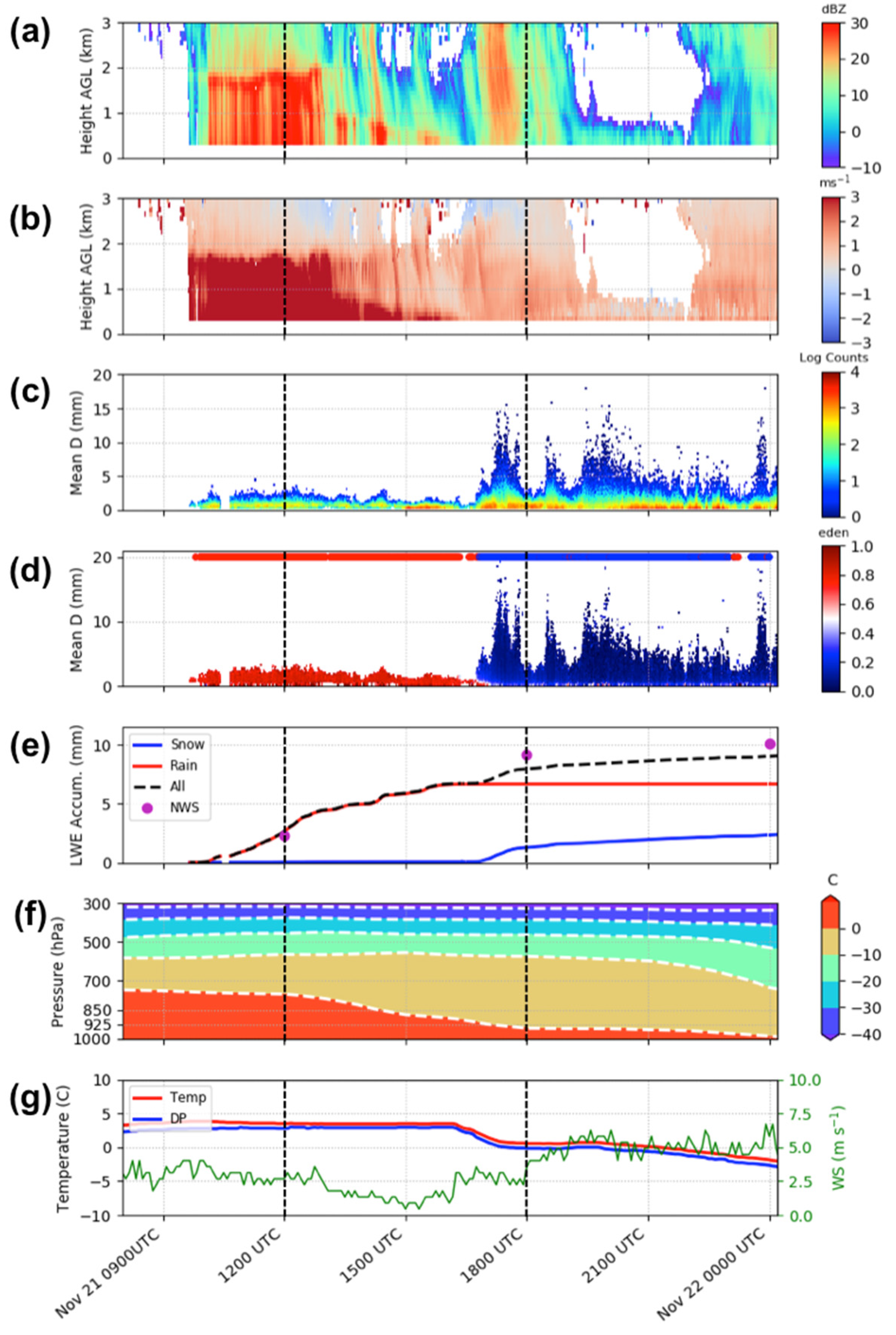
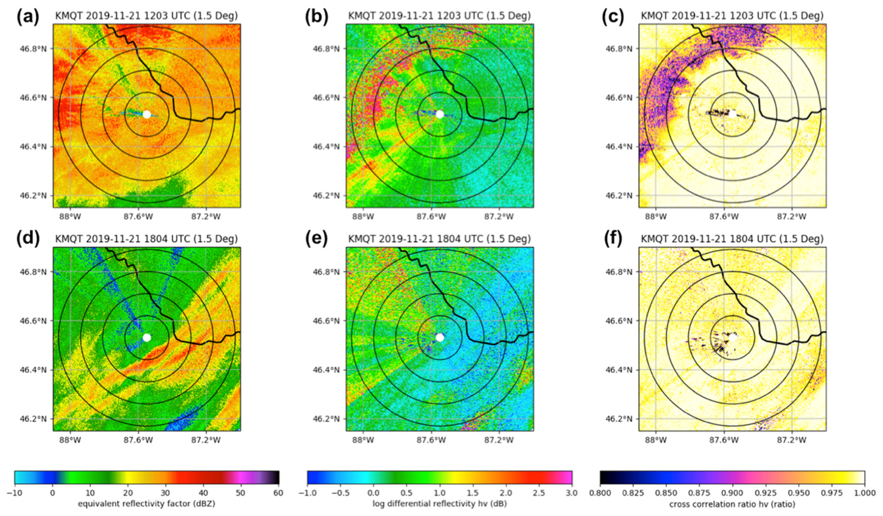
3.2.1. Rain-to-Snow Transition Events
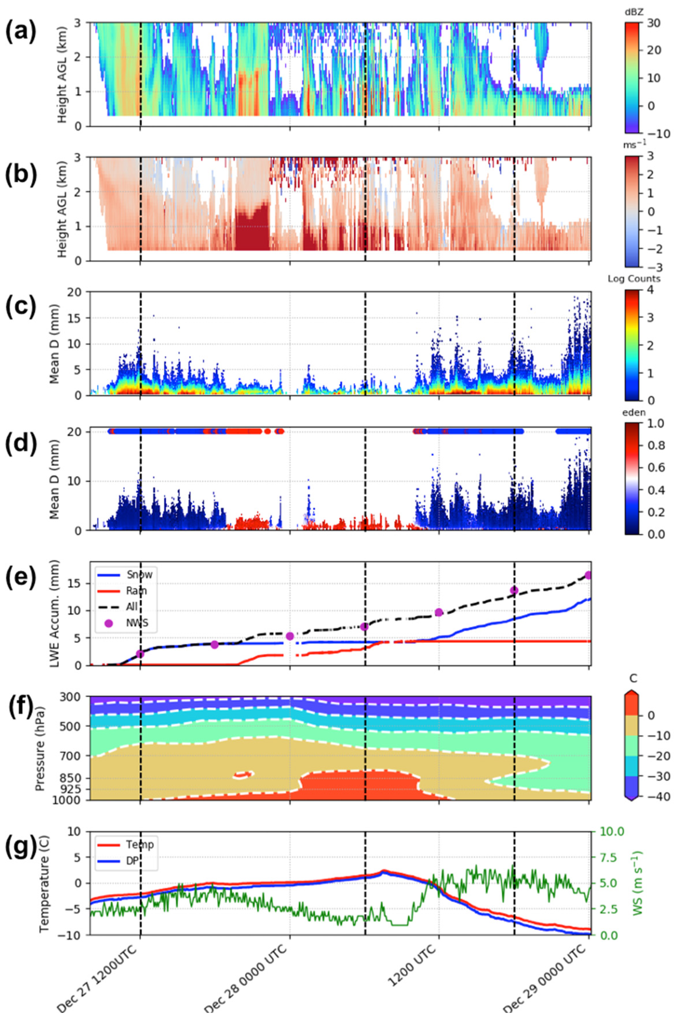
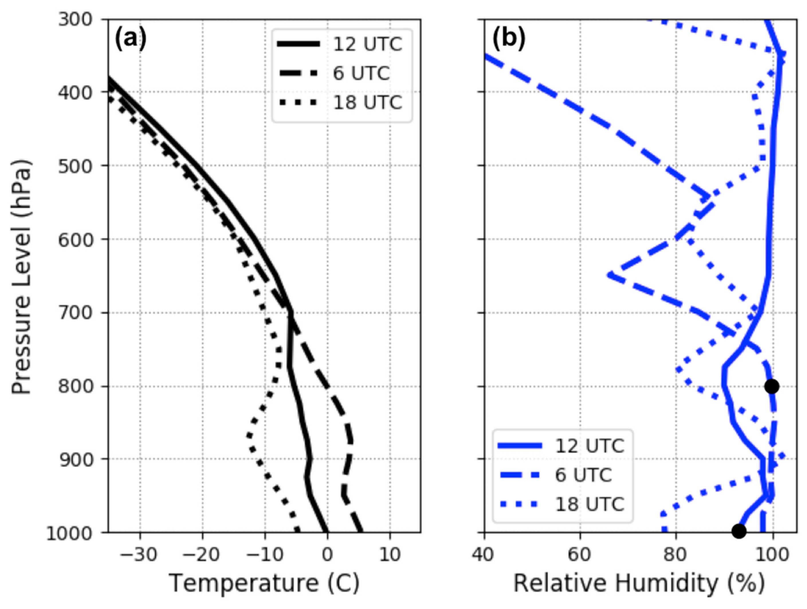
3.2.2. Snow-to-Rain-to-Snow Transition Event
3.2.3. Mixed-Phase Precipitation Event
4. Discussion
5. Conclusions
Author Contributions
Funding
Data Availability Statement
Acknowledgments
Conflicts of Interest
References
- Uccellini, L.W.; Kocin, P.J. The interaction of jet streak circulations during heavy snow events along the east coast of the United States. Weather Forecast. 1987, 2, 289–308. [Google Scholar] [CrossRef] [Green Version]
- Kocin, P.J.; Schumacher, P.N.; Morales, R.F., Jr.; Uccellini, L.W. Overview of the 12–14 March 1993 superstorm. Bull. Am. Meteorol. Soc. 1995, 76, 165–182. [Google Scholar] [CrossRef] [Green Version]
- Maglaras, G.J.; Waldstreicher, J.S.; Kocin, P.J.; Gigi, A.F.; Marine, R.A. Winter weather forecasting throughout the eastern United States. Part I: An overview. Weather Forecast. 1995, 10, 5–20. [Google Scholar] [CrossRef] [Green Version]
- Uccellini, L.W.; Kocin, P.J.; Schneider, R.S.; Stokols, P.M.; Dorr, R.A. Forecasting the 12–14 March 1993 superstorm. Bull. Am. Meteorol. Soc. 1995, 76, 183–200. [Google Scholar] [CrossRef] [Green Version]
- Keeter, K.K.; Businger, S.; Lee, L.G.; Waldstreicher, J.S. Winter weather forecasting throughout the eastern United States. Part III: The effects of topography and the variability of winter weather in the Carolinas and Virginia. Weather Forecast. 1995, 10, 42–60. [Google Scholar] [CrossRef] [Green Version]
- Musselman, K.N.; Lehner, F.; Ikeda, K.; Clark, M.P.; Prein, A.F.; Liu, C.; Barlage, M.; Rasmussen, R. Projected increases and shifts in rain-on-snow flood risk over western North America. Nat. Clim. Chang. 2018, 8, 808–812. [Google Scholar] [CrossRef]
- Suriano, Z.J.; Leathers, D.J.; Benjamin, A.E. Regionalization of Northeast US moisture conditions: Analysis of synoptic-scale atmospheric drivers. Clim. Res. 2020, 79, 193–206. [Google Scholar] [CrossRef]
- Li, Q.; Yang, T.; Zhou, H.; Li, L. Patterns in snow depth maximum and snow cover days during 1961–2015 period in the Tianshan Mountains, Central Asia. Atmos. Res. 2019, 228, 14–22. [Google Scholar] [CrossRef]
- Wachowicz, L.J.; Mote, T.L.; Henderson, G.R. A rain on snow climatology and temporal analysis for the eastern United States. Phys. Geogr. 2020, 41, 54–69. [Google Scholar] [CrossRef]
- Arigony-Neto, J.; Saurer, H.; Simões, J.C.; Rau, F.; Jaña, R.; Vogt, S.; Gossmann, H. Spatial and temporal changes in dry-snow line altitude on the Antarctic Peninsula. Clim. Chang. 2009, 94, 19–33. [Google Scholar] [CrossRef]
- Hantel, M.; Maurer, C.; Mayer, D. The snowline climate of the Alps 1961–2010. Theor. Appl. Climatol. 2012, 110, 517–537. [Google Scholar] [CrossRef] [Green Version]
- Fabry, F.; Zawadzki, I. Long-term radar observations of the melting layer of precipitation and their interpretation. J. Atmos. Sci. 1995, 52, 838–851. [Google Scholar] [CrossRef]
- Vivekanandan, J.; Zrnic, D.S.; Ellis, S.M.; Oye, R.; Ryzhkov, A.V.; Straka, J. Cloud microphysics retrieval using S-band dual-polarization radar measurements. Bull. Am. Meteorol. Soc. 1999, 80, 381–388. [Google Scholar] [CrossRef]
- Lim, J.O.J.; Hong, S.Y. Effects of bulk ice microphysics on the simulated monsoonal precipitation over East Asia. J. Geophys. Res. Atmos. 2005, 110. [Google Scholar] [CrossRef] [Green Version]
- Maahn, M.; Burgard, C.; Crewell, S.; Gorodetskaya, I.V.; Kneifel, S.; Lhermitte, S.; Van Tricht, K.; van Lipzig, N.P. How does the spaceborne radar blind zone affect derived surface snowfall statistics in polar regions? J. Geophys. Res. Atmos. 2014, 119, 13–604. [Google Scholar] [CrossRef] [Green Version]
- Norin, L.; Devasthale, A.; L’Ecuyer, T.S.; Wood, N.B.; Smalley, M. Intercomparison of snowfall estimates derived from the CloudSat Cloud Profiling Radar and the ground-based weather radar network over Sweden. Atmos. Meas. Tech. 2015, 8, 5009–5021. [Google Scholar] [CrossRef] [Green Version]
- Casella, D.; Panegrossi, G.; Sanò, P.; Marra, A.C.; Dietrich, S.; Johnson, B.T.; Kulie, M.S. Evaluation of the GPM-DPR snowfall detection capability: Comparison with CloudSat-CPR. Atmos. Res. 2017, 197, 64–75. [Google Scholar] [CrossRef]
- Kummerow, C.D.; Randel, D.L.; Kulie, M.; Wang, N.Y.; Ferraro, R.; Joseph Munchak, S.; Petkovic, V. The evolution of the Goddard profiling algorithm to a fully parametric scheme. J. Atmos. Ocean. Technol. 2015, 32, 2265–2280. [Google Scholar] [CrossRef]
- Zhang, J.; Howard, K.; Langston, C.; Vasiloff, S.; Kaney, B.; Arthur, A.; Van Cooten, S.; Kelleher, K.; Kitzmiller, D.; Ding, F.; et al. National Mosaic and Multi-Sensor QPE (NMQ) system: Description, results, and future plans. Bull. Am. Meteorol. Soc. 2011, 92, 1321–1338. [Google Scholar] [CrossRef] [Green Version]
- Sims, E.M.; Liu, G. A parameterization of the probability of snow–rain transition. J. Hydrometeorol. 2015, 16, 1466–1477. [Google Scholar] [CrossRef]
- Burdanowitz, J.; Klepp, C.; Bakan, S. An automatic precipitation-phase distinction algorithm for optical disdrometer data over the global ocean. Atmos. Meas. Tech. 2016, 9, 1637–1652. [Google Scholar] [CrossRef] [Green Version]
- Kochendorfer, J.; Nitu, R.; Wolff, M.; Mekis, E.; Rasmussen, R.; Baker, B.; Earle, M.E.; Reverdin, A.; Wong, K.; Smith, C.D.; et al. Testing and development of transfer functions for weighing precipitation gauges in WMO-SPICE. Hydrol. Earth Syst. Sci. 2018, 22, 1437. [Google Scholar] [CrossRef] [Green Version]
- Rasmussen, R.; Baker, B.; Kochendorfer, J.; Meyers, T.; Landolt, S.; Fischer, A.P.; Black, J.; Thériault, J.M.; Kucera, P.; Gochis, D.; et al. How well are we measuring snow: The NOAA/FAA/NCAR winter precipitation test bed. Bull. Am. Meteorol. Soc. 2012, 93, 811–829. [Google Scholar] [CrossRef] [Green Version]
- Löffler-Mang, M.; Joss, J. An optical disdrometer for measuring size and velocity of hydrometeors. J. Atmos. Ocean. Technol. 2000, 17, 130–139. [Google Scholar] [CrossRef]
- Wayand, N.E.; Stimberis, J.; Zagrodnik, J.P.; Mass, C.F.; Lundquist, J.D. Improving simulations of precipitation phase and snowpack at a site subject to cold air intrusions: Snoqualmie Pass, WA. J. Geophys. Res. Atmos. 2016, 121, 9929–9942. [Google Scholar] [CrossRef]
- Tokay, A.; Wolff, D.B.; Petersen, W.A. Evaluation of the new version of the laser-optical disdrometer, OTT Parsivel2. J. Atmos. Ocean. Technol. 2014, 31, 1276–1288. [Google Scholar] [CrossRef]
- Dolan, B.; Fuchs, B.; Rutledge, S.A.; Barnes, E.A.; Thompson, E.J. Primary modes of global drop size distributions. J. Atmos. Sci. 2018, 75, 1453–1476. [Google Scholar] [CrossRef]
- Park, S.G.; Kim, H.L.; Ham, Y.W.; Jung, S.H. Comparative evaluation of the OTT PARSIVEL2 using a collocated two-dimensional video disdrometer. J. Atmos. Ocean. Technol. 2017, 34, 2059–2082. [Google Scholar] [CrossRef]
- Battaglia, A.; Rustemeier, E.; Tokay, A.; Blahak, U.; Simmer, C. PARSIVEL snow observations: A critical assessment. J. Atmos. Ocean. Technol. 2010, 27, 333–344. [Google Scholar] [CrossRef]
- Newman, A.J.; Kucera, P.A.; Bliven, L.F. Presenting the snowflake video imager (SVI). J. Atmos. Ocean. Tech. 2009, 26, 167–179. [Google Scholar] [CrossRef]
- Pettersen, C.; Bliven, L.F.; von Lerber, A.; Wood, N.B.; Kulie, M.S.; Mateling, M.E.; Moisseev, D.N.; Munchak, S.J.; Petersen, W.A.; Wolff, D.B. The Precipitation Imaging Package: Assessment of Microphysical and Bulk Characteristics of Snow. Atmosphere 2020, 11, 785. [Google Scholar] [CrossRef]
- Pettersen, C.; Kulie, M.S.; Bliven, L.F.; Merrelli, A.J.; Petersen, W.A.; Wagner, T.J.; Wolff, D.B.; Wood, N.B. A composite analysis of snowfall modes from four winter seasons in Marquette, Michigan. J. Appl. Meteorol. Climatol. 2020, 59, 103–124. [Google Scholar] [CrossRef]
- Kulie, M.S.; Pettersen, C.; Merrelli, A.J.; Wagner, T.J.; Wood, N.B.; Dutter, M.; Beachler, D.; Kluber, T.; Turner, R.; Mateling, M.; et al. Snowfall in the Northern Great Lakes: Lessons Learned from a Multi-Sensor Observatory. Bull. Am. Meteorol. Soc. 2021, 1–61. [Google Scholar] [CrossRef]
- Hou, A.Y.; Kakar, R.K.; Neeck, S.; Azarbarzin, A.A.; Kummerow, C.D.; Kojima, M.; Oki, R.; Nakamura, K.; Iguchi, T. The global precipitation measurement mission. Bull. Am. Meteorol. Soc. 2014, 95, 701–722. [Google Scholar] [CrossRef]
- von Lerber, A.; Moisseev, D.; Bliven, L.F.; Petersen, W.; Harri, A.M.; Chandrasekar, V. Microphysical properties of snow and their link to Z e–S relations during BAECC 2014. J. Appl. Meteor. Clim. 2017, 56, 1561–1582. [Google Scholar] [CrossRef]
- Klugmann, D.; Heinsohn, K.; Kirtzel, H.J. A low cost 24 GHz FM-CW Doppler radar rain profiler. Contrib. Atmos. Phys. 1996, 61, 247–253. [Google Scholar]
- Peters, G.; Fischer, B.; Andersson, T. Rain observations with a vertically looking Micro Rain Radar (MRR). Boreal Environ. Res. 2002, 7, 353–362. [Google Scholar]
- Kneifel, S.; Maahn, M.; Peters, G.; Simmer, C. Observation of snowfall with a low-power FM-CW K-band radar (Micro Rain Radar). Meteorol. Atmos. Phys. 2011, 113, 75–87. [Google Scholar] [CrossRef] [Green Version]
- Maahn, M.; Kollias, P. Improved Micro Rain Radar snow measurements using Doppler spectra post-processing. Atmos. Meas. Tech. 2012, 5, 2661–2673. [Google Scholar] [CrossRef] [Green Version]
- Stull, R. Wet-bulb temperature from relative humidity and air temperature. J. Appl. Meteorol. Climatol. 2011, 50, 2267–2269. [Google Scholar] [CrossRef] [Green Version]
- Hersbach, H.; Bell, B.; Berrisford, P.; Hirahara, S.; Horányi, A.; Muñoz-Sabater, J.; Nicolas, J.; Peubey, C.; Radu, R.; Schepers, D.; et al. The ERA5 global reanalysis. Q. J. R. Meteorol. Soc. 2020, 146, 1999–2049. [Google Scholar] [CrossRef]
- Atlas, D.; Ulbrich, C.W. Path-and area-integrated rainfall measurement by microwave attenuation in the 1–3 cm band. J. Appl. Meteorol. 1977, 16, 1322–1331. [Google Scholar] [CrossRef] [Green Version]
- Heymsfield, A.J.; Bansemer, A.; Schmitt, C.; Twohy, C.; Poellot, M.R. Effective ice particle densities derived from aircraft data. J. Atmos. Sci. 2004, 61, 982–1003. [Google Scholar] [CrossRef]
- Herzegh, P.H.; Jameson, A.R. Observing precipitation through dual-polarization radar measurements. Bull. Am. Meteorol. Soc. 1992, 73, 1365–1376. [Google Scholar] [CrossRef] [Green Version]
- Ryzhkov, A.V.; Zrnic, D.S. Discrimination between rain and snow with a polarimetric radar. J. Appl. Meteorol. 1998, 37, 1228–1240. [Google Scholar] [CrossRef]
- Matrosov, S.Y. Modeling backscatter properties of snowfall at millimeter wavelengths. J. Atmos. Sci. 2007, 64, 1727–1736. [Google Scholar] [CrossRef]
- Austin, P.M.; Bemis, A.C. A quantitative study of the “bright band” in radar precipitation echoes. J. Atmos. Sci. 1950, 7, 145–151. [Google Scholar] [CrossRef] [Green Version]


| Event Date | Precip. Phase | PIP Times | NWS Times | Precip. Phase | PIP Times | NWS Times |
|---|---|---|---|---|---|---|
| 10 February 2017 | Snow | 1035 UTC 1700 UTC | 1045 UTC 1715 UTC | Rain | 1648 UTC 1833 UTC | 1645 UTC 1830 UTC |
| 23 February 2017 | Rain | 0300 UTC 0425 UTC | 0300 UTC 0430 UTC | Snow | 0425 UTC 1108 UTC | 0430 UTC 1115 UTC |
| 27 April 2017 | Rain | 0745 UTC 1755 UTC | 0750 UTC 1750 UTC | Snow | 1753 UTC 2350 UTC | 1750 UTC 2345 UTC |
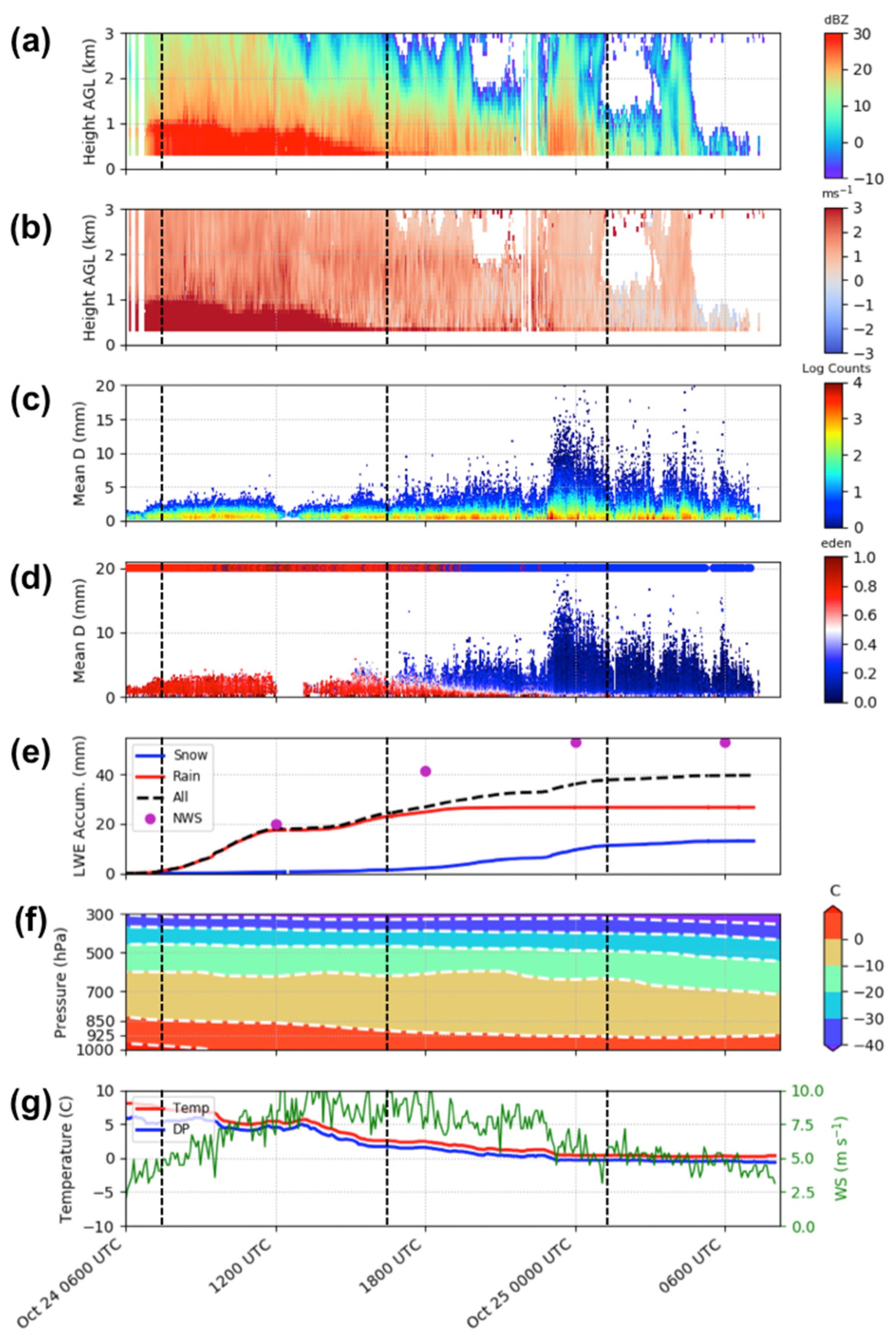
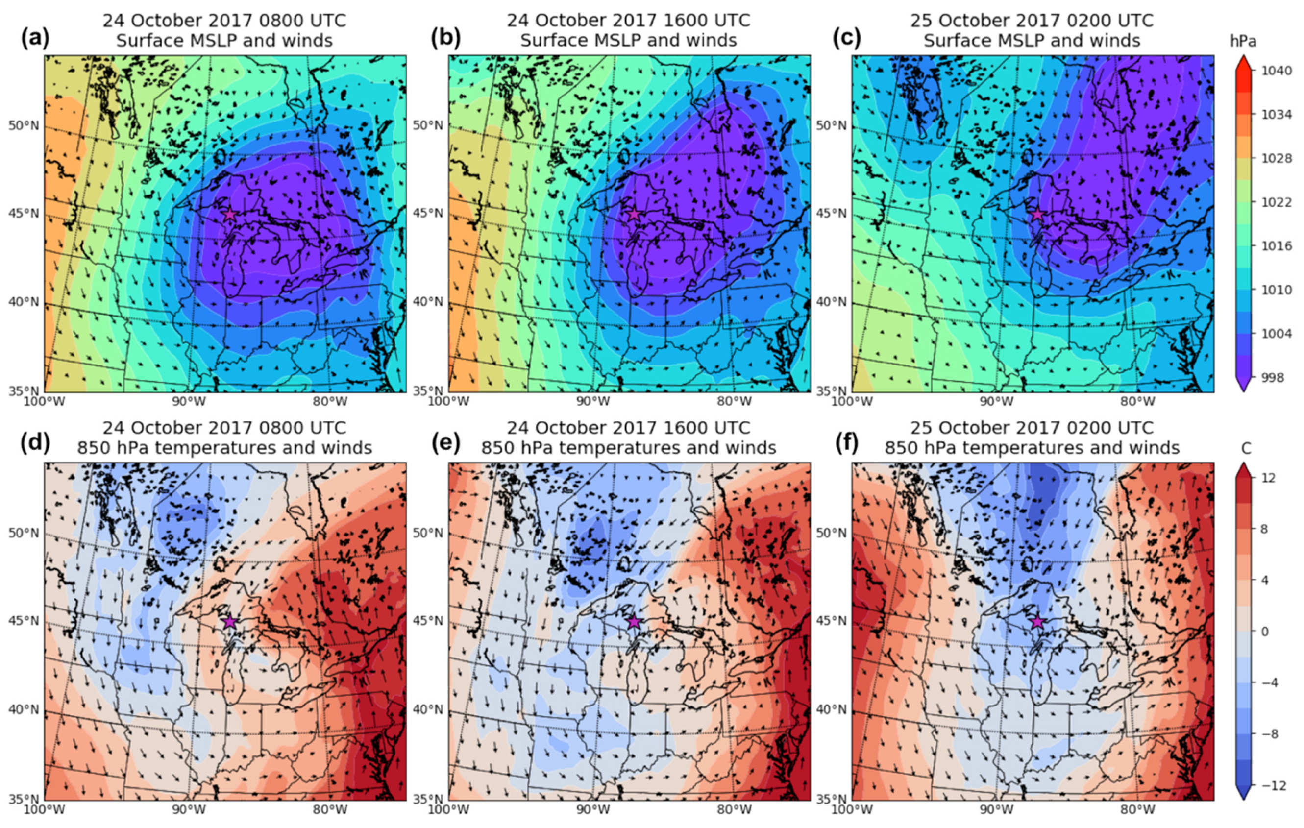
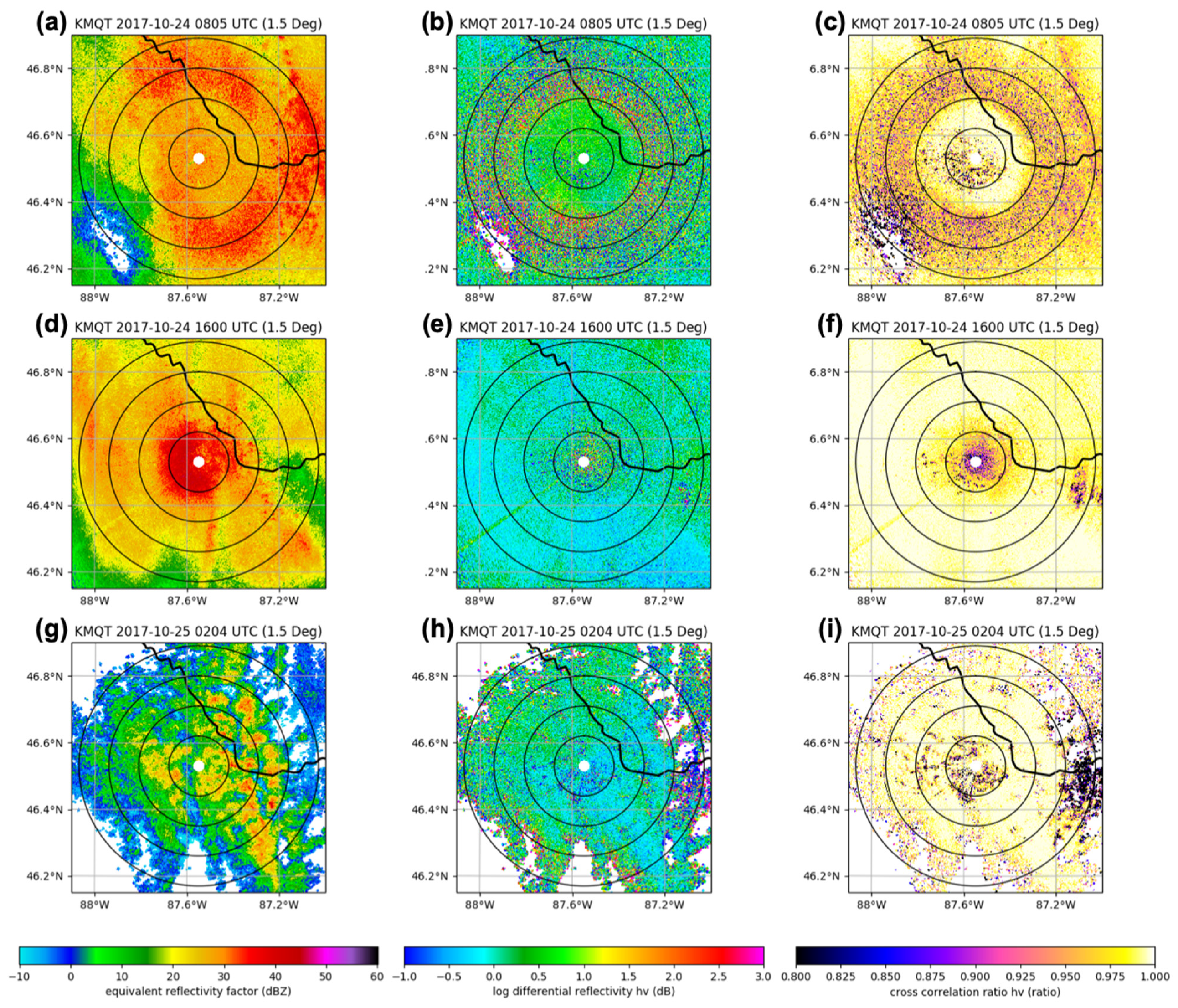
| 24 October 2017 | Rain | 0550 UTC 2130 UTC | 0600 UTC 2000 UTC | Snow/Mixed | 1515 UTC 0720 * UTC | 1525 UTC 0730 * UTC |
| 2 November 2017 | Snow | 0325 UTC 0820 UTC | 0250 UTC 0845 UTC | Rain | 0723 UTC 1035 UTC | 0730 UTC 1055 UTC |
| 5 December 2017 | Rain | 0250 UTC 0945 UTC | 0235 UTC 0950 UTC | Snow | 1000 UTC 1230 UTC | 1015 UTC 1215 UTC |
| 11 January 2018 | Rain | 1440 UTC 1655 UTC | 1445 UTC 1645 UTC | Snow | 1630 UTC 0000 * UTC | 1625 UTC 0000 * UTC |
| 7 November 2018 | Rain | 0035 UTC 0835 UTC | 0050 UTC 0835 UTC | Snow | 0615 UTC 2125 UTC | 0635 UTC 2110 UTC |
| 11 April 2019 | Snow | 1945 UTC 0255 * UTC | 1945 UTC 0300 UTC | Rain/Mixed | 1930 UTC 0820 * UTC | 1945 UTC 0815 * UTC |
| 21 November 2019 | Rain | 0940 UTC 1700 UTC | 0940 UTC 1650 UTC | Snow | 1650 UTC 0000 * UTC | 1650 UTC 0000 * UTC |
| 30 December 2019 | Rain | 0855 UTC 1120 UTC | 0900 UTC 1110 UTC | Snow | 1105 UTC 2100 UTC | 1110 UTC 2100 UTC |
| Event Date | Precip. Phase | PIP Times | NWS Times | Precip. Phase | PIP Times | NWS Times | Precip. Phase | PIP Times | NWS Times |
|---|---|---|---|---|---|---|---|---|---|
| 17 November 2017 | Snow | 1255 UTC 1450 UTC | 1300 UTC 1435 UTC | Rain | 1645 UTC 2345 UTC | 1630 UTC 2350 UTC | Snow | 2345 UTC 0300 * UTC | 2350 UTC 0300 * UTC |
| 27 December 2018 | Snow | 0930 UTC 1855 UTC | 0925 UTC 1910 UTC | Rain | 1955 UTC 1030 * UTC | 2100 UTC 1015 * UTC | Snow | 1005 * UTC 0125 ** UTC | 1015 * UTC 0130 ** UTC |
| Event Date | PIP LWE (mm) | NWS LWE (mm) | Diff. % PIP–NWS | Mean WS (m s−1) | Max WS (m s−1) |
|---|---|---|---|---|---|
| 10 February 2017 1000–1800 UTC | 2.32 | 2.54 | −9.4 | 3.94 | 5.81 |
| 23 February 2017 0200–1200 UTC | 11.01 | 10.16 | 7.7 | 3.57 | 5.36 |
| 27 April 2017 0800–0000 * UTC | 17.58 | 17.78 | −1.1 | 0.33 | 0.83 |
| 24 October 2017 0600–0800 * UTC | 39.71 | 53.34 | −34.3 | 6.78 | 12.07 |
| 2 November 2017 0300–1200 UTC | 3.23 | 3.55 | −9.9 | 1.33 | 2.68 |
| 17 November 2017 1200–0600 * UTC | 8.53 | 7.87 | 7.7 | 2.66 | 5.36 |
| 5 December 2017 0200–1200 UTC | 4.74 | 4.57 | 3.6 | 6.05 | 11.17 |
| 11 January 2018 1400–0000 * UTC | 9.90 | 9.65 | 2.5 | 2.76 | 6.23 |
| 7 November 2018 1000–0000 ** UTC | 3.74 | 3.56 | 4.8 | 3.62 | 5.81 |
| 27 December 2018 0000–0000 ** UTC | 16.97 | 16.51 | 2.7 | 3.41 | 6.71 |
| 11 April 2019 1800–1200 * UTC | 34.59 | 32.26 | 6.7 | 3.29 | 6.71 |
| 21 November 2019 1000–0000 * UTC | 9.31 | 10.16 | −9.1 | 3.29 | 6.23 |
| 30 December 2019 0800–2100 UTC | 24.03 | 23.11 | 3.8 | 2.32 | 4.02 |
| Time | Wet Bulb (°C) | Lapse Rate (°C km−1) | Probability of Solid Precipitation | Precipitation Phase (PIP) |
|---|---|---|---|---|
| 11 January 2018 | ||||
| 1500 UTC | 1.2 | 5.0 | 30% | Rain |
| 1700 UTC | 0.8 | 5.5 | 40% | Snow |
| 1900 UTC | −2.0 | 6.4 | >90% | Snow |
| 2100 UTC | −6.5 | 8.8 | 100% | Snow |
| 21 November 2019 | ||||
| 1500 UTC | 3.0 | 5.2 | <10% | Rain |
| 1800 UTC | 0.2 | 6.2 | >80% | Snow |
| 27 December 2018 | ||||
| 1200 UTC | −2.8 | 2.5 | >90% | Snow |
| 1800 UTC | −1.0 | 6.8 | >90% | Rain |
| 0000 UTC* | 0.0 | 4.8 | 80% | Rain |
| 0600 UTC* | 1.0 | 3.1 | 30% | Rain |
| 1800 UTC* | −7.0 | 10.0 | 100% | Snow |
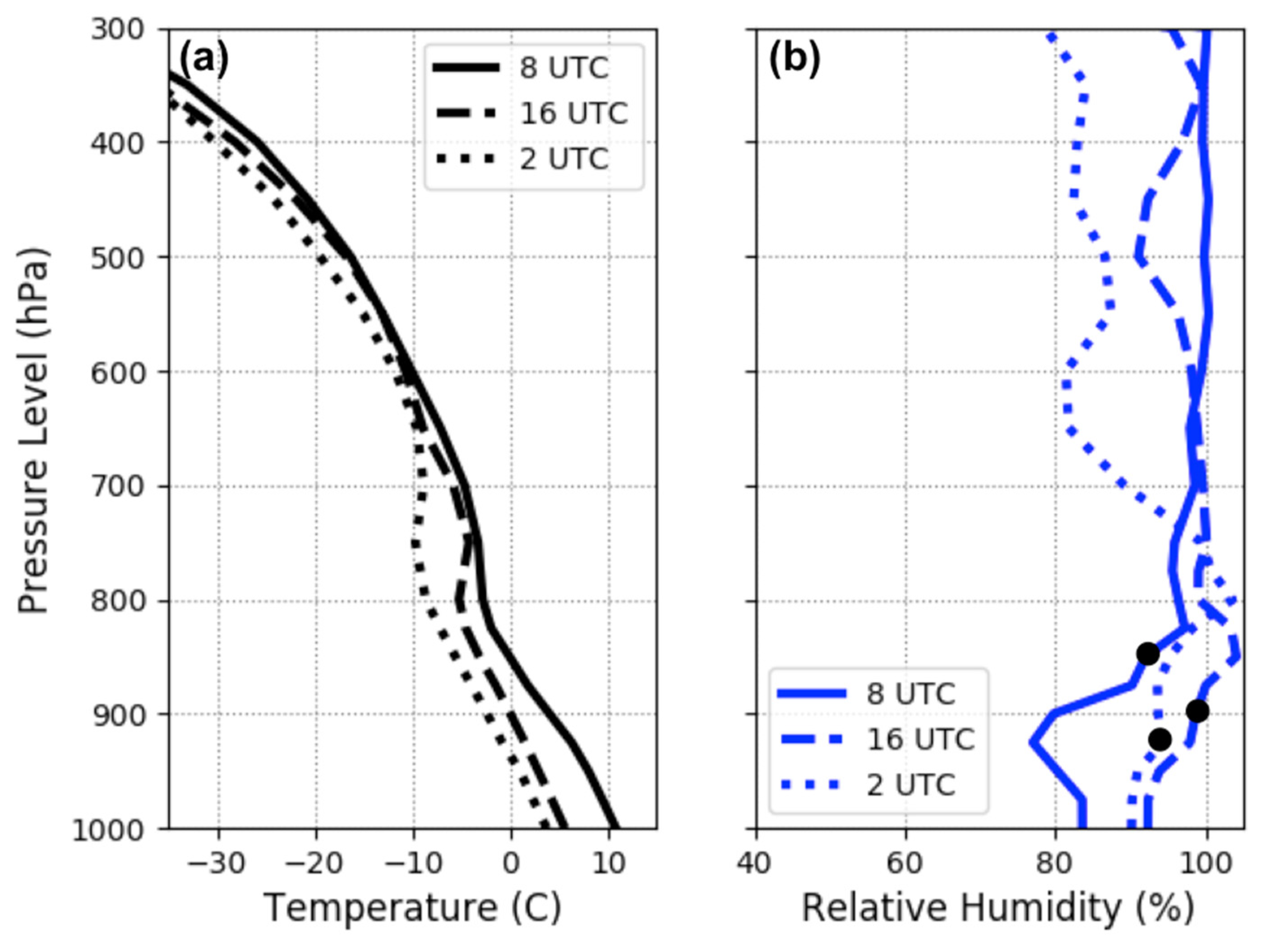
| 24 October 2017 | ||||
| 0800 UTC | 6.0 | 7.2 | <10% | Rain |
| 1600 UTC | 2.0 | 6.5 | 10% | Rain |
| 1800 UTC | 1.8 | 6.5 | 10% | Mixed |
| 2000 UTC | 1.2 | 7.0 | 40% | Mixed |
| 2200 UTC | 0.8 | 7.2 | 60% | Mixed |
| 0200 UTC * | 0.0 | 7.5 | 80% | Snow |
Publisher’s Note: MDPI stays neutral with regard to jurisdictional claims in published maps and institutional affiliations. |
© 2021 by the authors. Licensee MDPI, Basel, Switzerland. This article is an open access article distributed under the terms and conditions of the Creative Commons Attribution (CC BY) license (https://creativecommons.org/licenses/by/4.0/).
Share and Cite
Pettersen, C.; Bliven, L.F.; Kulie, M.S.; Wood, N.B.; Shates, J.A.; Anderson, J.; Mateling, M.E.; Petersen, W.A.; von Lerber, A.; Wolff, D.B. The Precipitation Imaging Package: Phase Partitioning Capabilities. Remote Sens. 2021, 13, 2183. https://0-doi-org.brum.beds.ac.uk/10.3390/rs13112183
Pettersen C, Bliven LF, Kulie MS, Wood NB, Shates JA, Anderson J, Mateling ME, Petersen WA, von Lerber A, Wolff DB. The Precipitation Imaging Package: Phase Partitioning Capabilities. Remote Sensing. 2021; 13(11):2183. https://0-doi-org.brum.beds.ac.uk/10.3390/rs13112183
Chicago/Turabian StylePettersen, Claire, Larry F. Bliven, Mark S. Kulie, Norman B. Wood, Julia A. Shates, Jaclyn Anderson, Marian E. Mateling, Walter A. Petersen, Annakaisa von Lerber, and David B. Wolff. 2021. "The Precipitation Imaging Package: Phase Partitioning Capabilities" Remote Sensing 13, no. 11: 2183. https://0-doi-org.brum.beds.ac.uk/10.3390/rs13112183