The Potential of Landsat NDVI Sequences to Explain Wheat Yield Variation in Fields in Western Australia

Abstract

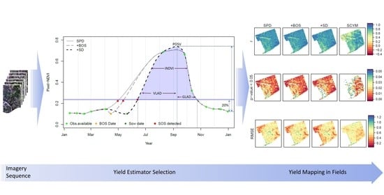
Long-term maps of within-field crop yield can help farmers understand how yield varies in time and space and optimise crop management. This study investigates the use of Landsat NDVI sequences for estimating wheat yields in fields in Western Australia (WA). By fitting statistical crop growth curves, identifying the timing and intensity of phenological events, the best single integrated NDVI metric in any year was used to estimate yield. The hypotheses were that: (1) yield estimation could be improved by incorporating additional information about sowing date or break of season in statistical curve fitting for phenology detection; (2) the integrated NDVI metrics derived from phenology detection can estimate yield with greater accuracy than the observed NDVI values at one or two time points only. We tested the hypotheses using one field (~235 ha) in the WA grain belt for training and another field (~143 ha) for testing. Integrated NDVI metrics were obtained using: (1) traditional curve fitting (SPD); (2) curve fitting that incorporates sowing date information (+SD); and (3) curve fitting that incorporates rainfall-based break of season information (+BOS). Yield estimation accuracy using integrated NDVI metrics was further compared to the results using a scalable crop yield mapper (SCYM) model. We found that: (1) relationships between integrated NDVI metrics using the three curve fitting models and yield varied from year to year; (2) overall, +SD marginally improved yield estimation (r = 0.81, RMSE = 0.56 tonnes/ha compared to r = 0.80, RMSE = 0.61 tonnes/ha using SPD), but +BOS did not show obvious improvement (r = 0.80, RMSE = 0.60 tonnes/ha); (3) use of integrated NDVI metrics was more accurate than SCYM (r = 0.70, RMSE = 0.62 tonnes/ha) on average and had higher spatial and yearly consistency with actual yield than using SCYM model. We conclude that sequences of Landsat NDVI have the potential for estimation of wheat yield variation in fields in WA but they need to be combined with additional sources of data to distinguish different relationships between integrated NDVI metrics and yield in different years and locations.

1. Introduction

Agriculture is Western Australia’s (WA) second-largest export industry, worth around AUD 8.5 billion per year, with wheat, canola and barley the top three products. Grain and oilseed crops are grown in the southwest, in a dryland system with crops dependent on winter rainfall [1,2]. The climate is variable, and it is becoming hotter and drier with climate change. Improving agricultural productivity and sustainability is important for the regional economy and for ensuring ongoing food security as the world’s population grows and the amount of arable land is threatened by competing land needs, degradation and climate change.

Precision agriculture (PA) aims to increase net profit per unit area of land and per unit of time in a sustainable manner [3]. In dryland cropping regions with considerable seasonal climate variability, such as the grain belt of Western Australia (WA), farmers practising PA aim to optimise crop management strategies in different parts of the field and in different growing seasons [4]. Long-term maps of within-field crop yield can potentially help farmers understand how yield varies in time and space according to different soil conditions and weather conditions, as well as management.

Satellite remote sensing offers a cost-effective and non-destructive means of estimating yield for the purpose of understanding spatial-temporal yield variability and supporting PA. While there are many choices of data sources, ranging from handheld radiometers to drones, airborne and satellite platforms, the Landsat series is well-suited for yield estimation to support PA management. It has a long-term record of satellite images dating back to 1982 [5], with global coverage at 30 m resolution which is sufficient for within-field monitoring. The revisit time is 16 days, which is well-suited for phenological monitoring. Moreover, Landsat data have been freely available since 2008 [6] and can therefore be used to offer inexpensive delivery of information to farmers at a scale suitable for making decisions about where and when management should be varied across a field.

Common practice for crop growth detection uses vegetation indices (VIs) that combine optical spectral reflectance measurements to maximise the discrimination of green vegetation from other types of land cover. For example, the normalised difference vegetation index (NDVI) measures the ratio of the difference between near-infrared (NIR) and red (RED) reflectance and their sum [7,8]. Time sequences of VIs are used to monitor crop development, fit statistical crop growth curves and identify the timing and intensity of phenological events [9,10,11,12,13]. Metrics derived from phenological growth curves, such as timing and degree of growth stages and time-integrated VIs, can then be used as predictors of yield [14,15,16,17]. However, their use is limited by the presence of clouds and cloud shadows, which occur more frequently during winter when crop growth is accelerated [18,19,20].

To overcome the challenges caused by pervasive clouds during the early-to mid-growing season in the time sequence of Landsat imagery, there are approaches to fuse Landsat with the data from satellites that revisit more frequently and/or have finer spatial resolution, e.g., Sentinel-2 [21] and MODIS [22], to retain the value of the past data archives. However, Sentinel-2 top-of-atmosphere products are available for Australasia only since December 2018 and cannot be used to produce long-term hindcasts and the coarser resolution of MODIS pixels has limited representativity of finer pixels because of saturation of mixed reflective signals, especially for investigating within field yield variability [23,24]. While Chen et al. [25] identified the threshold of clear-sky Landsat availability to use Landsat-MODIS blended data for crop yield prediction in Australia, the potential of using only Landsat observations to explain yield variation within fields is still unclear.

To avoid issues caused by cloud contamination, the scalable crop yield mapper (SCYM) [26] attempts to only use the cloud-free images acquired just prior to and after the peak of crop greenness to estimate yield. A crop simulation model, Agricultural Production Systems sIMulator (APSIM), is used to generate correlation coefficients between various combination of clear-sky green chlorophyll vegetation index (GCVI) and yields. The SCYM captures an average of 35% of maize yield variation at field-average level. At county-scale, the model’s explanatory power increases to 55%. However, SCYM accuracy has not been assessed at pixel (within-field) level because of limited ground truth availability.

In this study, we consider approaches that use additional on-farm information in the estimation of crop phenology from sequences of Landsat images to counter temporal gaps caused by winter cloud contamination. Due to the prevalence of rainy days before and after sowing date [4], the early part of the growth curve can be difficult to estimate. To alleviate this problem, we propose the use of farmer-provided records. In the WA grain belt, many farmers have accumulated long records of on-farm practices including their sowing and harvest dates. For farmers without records, sowing date can be estimated by the timing of rainfall events in Autumn with a common rule of thumb defining the break of season as occurring when 15 mm of rainfall is accumulated over three days after 25 April, or when 5 mm of rainfall accumulates over three days after 5 June [4]. We hypothesise that yield estimation using integrated NDVI metrics can be improved by incorporating additional information about sowing date or break of season in statistical curve fitting for phenology detection. From the application perspective of digital agriculture services, growers are often required to provide information for each field in the system, e.g., the field boundary. Providing information on sowing date, usually a common date for the whole field, can also be considered as user input. In addition, we hypothesise that the use of integrated NDVI metrics derived from phenology detection can estimate yield with greater accuracy than the SCYM model which uses VI at one or two time points only. The objectives of this study are: (1) to quantify the accuracy improvements on yield estimation by incorporating prior farming knowledge to traditional statistical phenology detection; (2) to investigate the best NDVI-derived predictors for spatial yield mapping; (3) to assess the potential of Landsat NDVI sequence for hindcasting long-term crop yield within field.

2. Date Collection and Pre-Processing

2.1. Study Fields, On-Farm Management Records, and Yield Maps

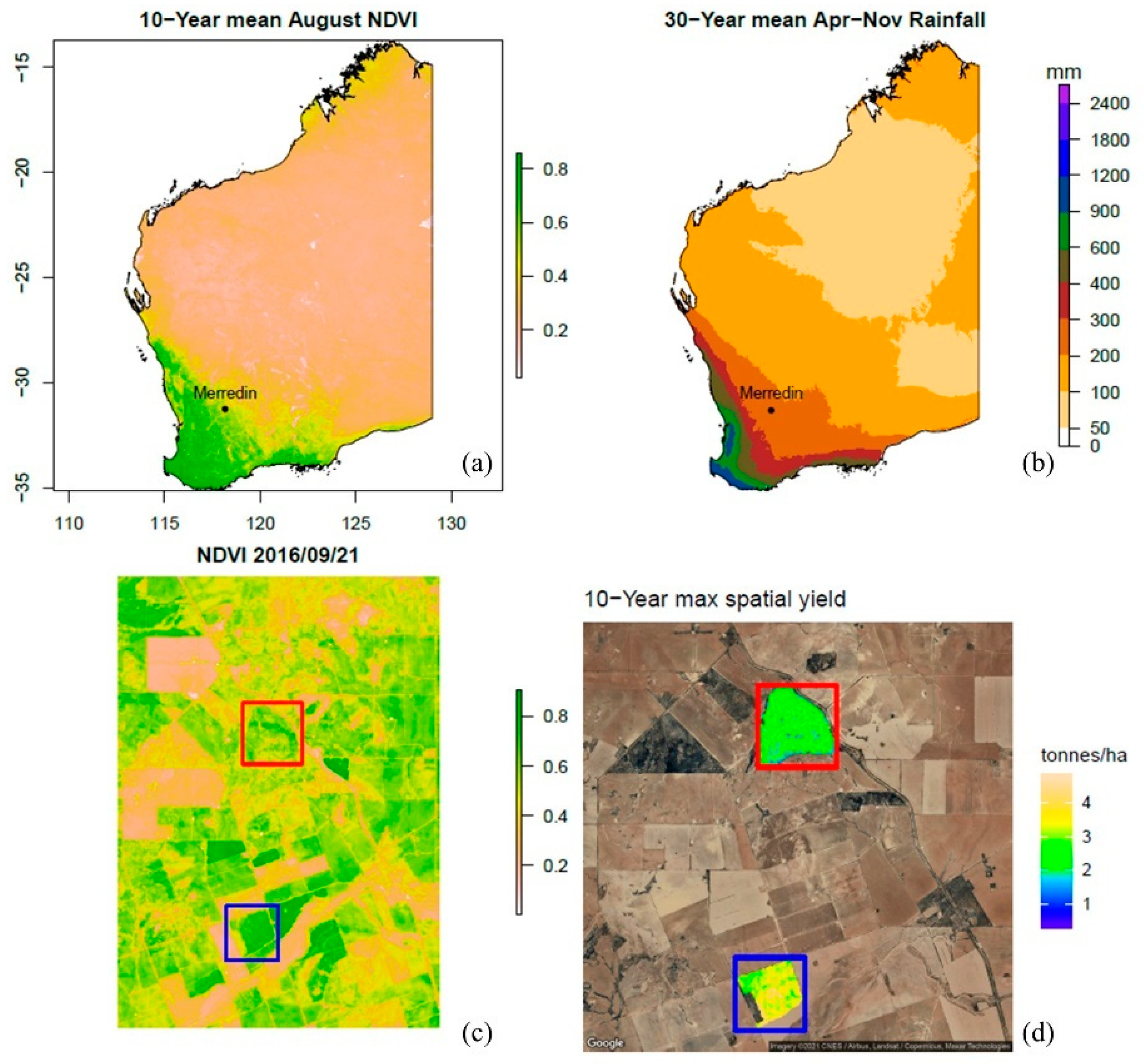
In Western Australia (WA), broadacre grain cropping relies heavily on winter rainfall [2,27]. The two study fields (Figure 1c,d, red box for J and blue box for M) are located in Merredin, the eastern wheat belt of WA (lower left latitudes/longitudes: 31.27°S/118.15°E and 31.33°S/118.15°E) with areas of ~235 ha and ~143 ha, respectively. Rainfall during the average winter crop growing season (April to November) is between 200–300 mm (Figure 1b). The climate is Mediterranean: wet in winter (June to August) and dry in summer (November to January). Using NDVI as a vegetation ‘greenness’ proxy, Figure 1a shows the spatial distribution of the winter crops in August, across WA. Figure 1c demonstrates spatial variation in vegetation growth around and within the study fields. The maximum wheat grain yield in 2003–2017 in the study fields ranged from 0.4 to 4.7 tonnes/ha (Figure 1d).

On-farm management information for both fields during 2003–2017 was collected from the farm owner. Crop yield maps were created from harvester yield monitor (YM) records. The YM has a 10.8 m of swath width and a logging interval of three seconds for an average distance of 7.7 ± 1.2 m. Dry yield mass (tonnes/ha) was used to represent actual on-farm yield. The data were pre-processed as follows: (1) remove outlier points in the upper 99% and lower 1% of the range in yield each year, (2) fit a spherical variogram model based on the cleaned yield data using ‘gstat’ package [28,29] and interpolate to a 30 m grid using kriging. In this study, we will only consider the pixels that are within the boundaries of the two fields. Pixels with at least three years of wheat yield records from the YM are shown in Figure 1d.

Table 1. Farming management and rainfall conditions for winter wheat in the two field sites during 2003 to 2017.

Year	Rainfall Available (mm)	Field	Yield (tons/ha)	Sow Date	Harvest Date
2003	331.4	J	2.055	21 May	15 January 2004
		M	3.194	12 May	12 December
2004	269.3	J	1.600	26 May	25 November
		M	1.610	10 June	18 December
2006	284.2	J	1.389	07 June	07 December
2007	172.9	J	0.483	31 May	05 November
		M	0.677	03 June	15 November
2009	258.0	J	1.195	01 June	07 December
		M	1.454	15 June	05 December
2012	178.4	J	0.467	24 June	21 December
		M	1.661	16 June	11 December
2013	271.2	J	1.835	15 May	20 November
		M	1.917	19 May	12 December
2015	235.5	J	--	23 May	05 December
2016	277.2	J	1.618	20 May	18 December
		M	2.031	18 May	08 December
2017	227.1	J	1.739	19 May	03 December
		M	1.691	23 May	23 November

‘Rainfall available’ was calculated as one-third of summer rainfall (December–March) plus general growing season rainfall (April–November).

shows that wheat has been planted in fields J and M for 10 and 8 years in 2003 to 2017, respectively.

2.2. Satellite Remote Sensing Datasets

We used Landsat 7 Enhanced Thematic Mapper Plus (ETM+) as the remote sensing data source as it covers the years 2003 to 2017. The scenes that overpass the study sites (path/row: 111/082) in the time window of 13 January 2003 to 24 December 2018 were collected from the United States Geological Survey website (USGS, https://earthexplorer.usgs.gov/ accessed on 2 February 2021). Initial pre-processing steps, including geometric correction, top of atmosphere reflectance correction, and surface reflectance correction were completed via the USGS Earth Resources Observation and Science (EROS) Centre Science Processing Architecture (ESPA) online interface (https://espa.cr.usgs.gov/ accessed on 3 February 2021). Thereafter, we removed pixels with cloud contamination on the basis of the pixel quality flags. We then calculated the normalized difference vegetation index (NDVI) and the green chlorophyll vegetation index (GCVI) time sequences based on the corrected surface reflectance (green, red and near-infrared) measurements for all the available time points (Equations (1) and (2)):

$$\mathrm{NDVI}=\frac{{\mathsf{\rho }}_{\mathrm{NIR}}-{\mathsf{\rho }}_{\mathrm{R}}}{{\mathsf{\rho }}_{\mathrm{NIR}}-{\mathsf{\rho }}_{\mathrm{R}}}$$

(1)

$$\mathrm{GCVI}=\frac{{\mathsf{\rho }}_{\mathrm{NIR}}}{{\mathsf{\rho }}_{\mathrm{GRN}}}-1$$

(2)

where ${\mathsf{\rho }}_{\mathrm{NIR}}$, ${\mathsf{\rho }}_{\mathrm{R}}$ and ${\mathsf{\rho }}_{\mathrm{GRN}}$ are the near-infrared (0.77–0.90 µm), red (0.63–0.69 µm), and green (0.52–0.60 µm) wavelength reflectances, respectively.

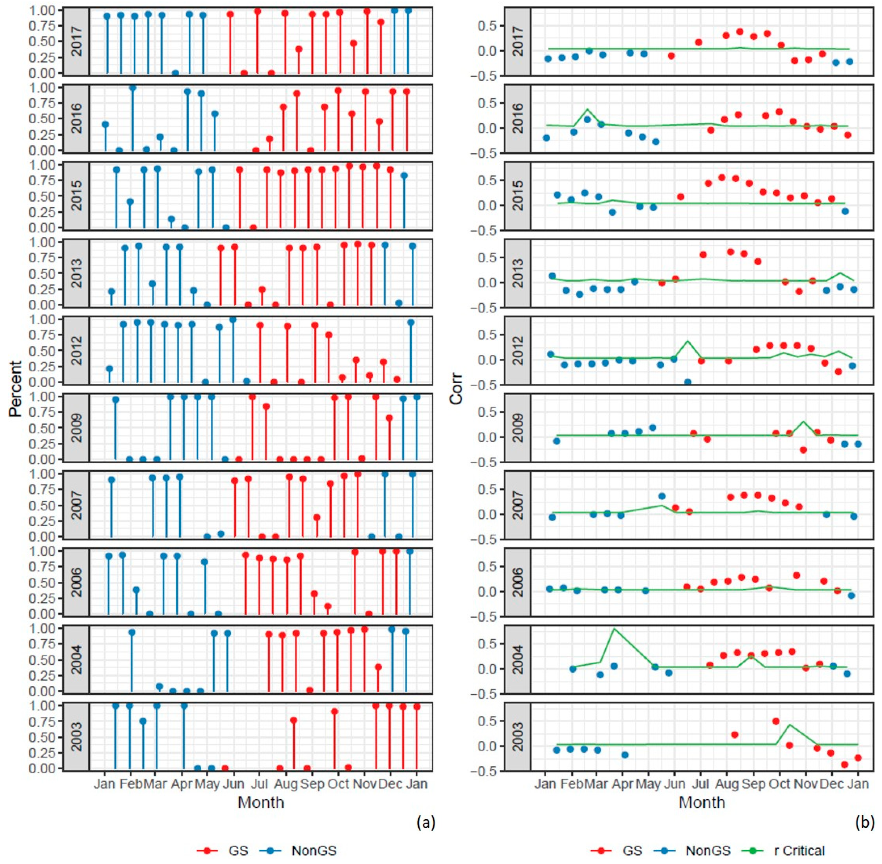
In order to assess the availability of Landsat 7 imagery for the study sites, we counted the number of available images both in the farmer-reported growing season (sowing date to harvest date) and the whole year, and also the percentage of clear-sky pixels out of the total wheat crop pixels each year. In addition, we calculated the correlation coefficients (r) between clear-sky NDVI at each image acquisition date with yield each year; The critical value of ‘r Critical’ was calculated based on the number of available clear-sky pixels (the lower the number, the higher the ‘r Critical’) at significance level, p value = 0.05. We only show positive correlations in this study. Thus, the correlation (r) was statistically significant when it is greater than its corresponding ‘r Critical’.

2.3. Climate Data

Historical climate daily data (1 January 1975 to 31 December 2018) for Merredin were accessed from the Nungarin weather station site (Lat/Lon 31.18°S/118.10°E, 292 m in elevation) from the Long Paddock Australian climate database (https://www.longpaddock.qld.gov.au/silo accessed on 3 February 2021). Break of season dates were calculated from daily rainfall data using the rule: the date when 15 mm of rainfall was accumulated over 3 days after 25 April, or 5 mm over 3 days after 5 June [4].

3. Methodology

3.1. Models Tested

We tested four models for yield estimation (

Table 2. Summary of crop models to be tested for yield estimation in this study from 2003 to 2017.

Model	Predictors of Yield	Abbreviation
Statistical phenology detection	Single best phenological metric each year	SPD
Statistics phenology detection with added sowing date information	Single best phenological metric each year	+SD
Statistical phenology detection with added break of season information	Single best phenological metric each year	+BOS
Scalable crop yield mapper	NDVI values from one or two time points	SCYM

): (1) statistical phenology detection model (SPD) as commonly performed; (2) statistical phenology detection model incorporating sowing date information (+SD); (3) statistical phenology detection incorporating break of season date (+BOS); and (4) the SCYM model. Section 3.1.1 describes the methods used to perform SPD and extract integrated NDVI metrics. Section 3.1.2 describes how additional information is used in the +SD and +BOS models. Section 3.1.3 describes how the integrated NDVI metrics generated from the three methods for phenology detection (SPD, +SD and +BOS) were used to estimate yield. Section 3.1.4 describes the SCYM model.

3.1.1. Statistical Phenology Detection (SPD)

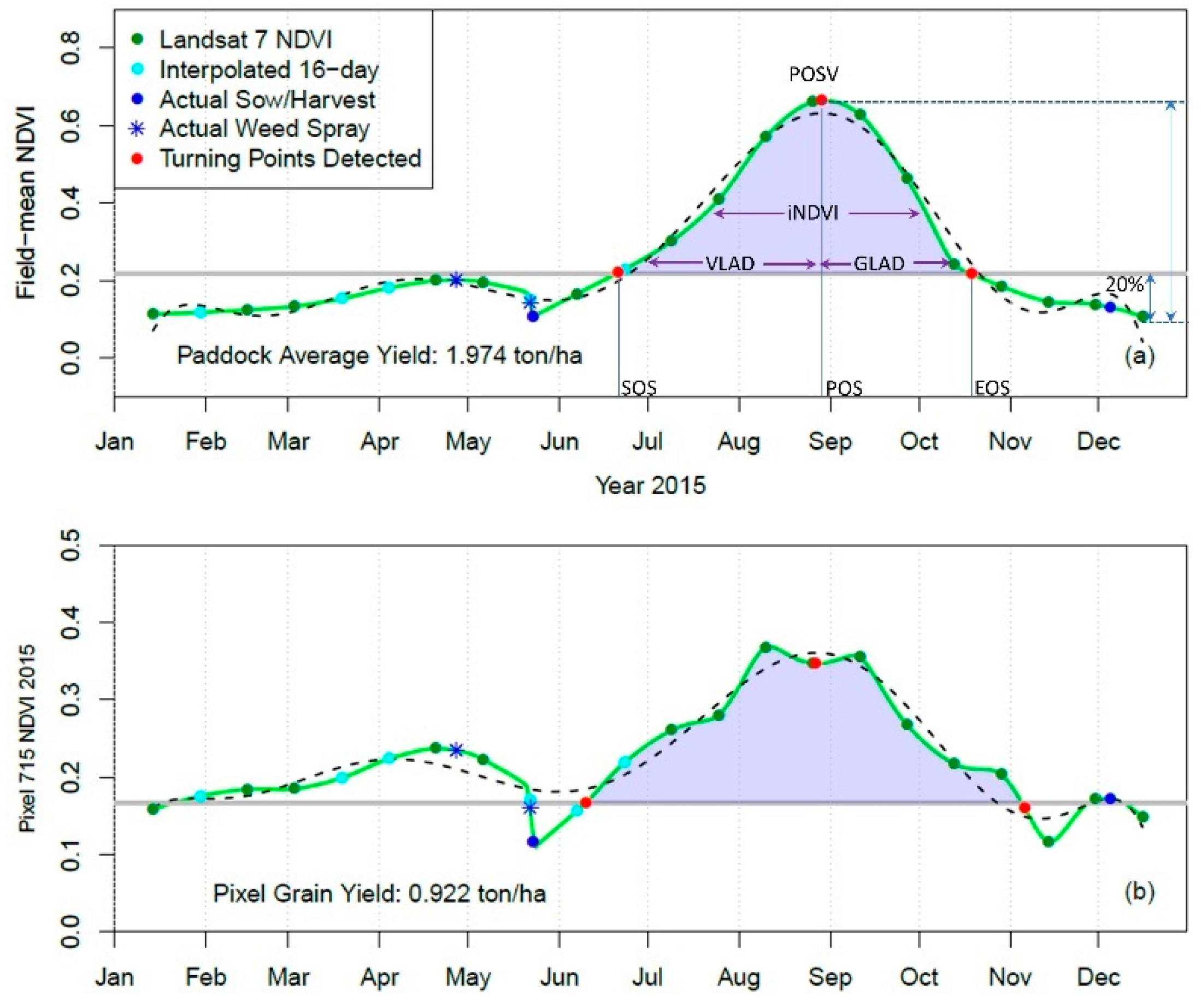
The SPD model composites commonly adopted methodology for fitting curves to NDVI time sequences. The process includes data interpolation and smoothing, turning points determination, and integrated metrics calculation [9,10,11,12]. Specific steps were configured from the pixel-by-pixel check at field J (see Supplementary Materials File S1 for detailed examples). The steps are:

(1)

Fill missing values in the 16-day time sequence of NDVI using the Stineman interpolation method [30]. The Stineman interpolation method is a consistently well-behaved method where the interpolated curve passes through the original points and exactly matches the given slopes at those points [31];

(2)

Repeat step 1 to interpolate the 16-day time-series NDVI to daily sequence. As a result, the daily reconstructed NDVI series was named as ‘reconstructed daily’ in the following analysis;

(3)

Fit a multi-polynomial with a degree of 8 to the ‘reconstructed daily’ sequences for each year to identify the peak of season (POS) date. While POSV is the value in the ‘reconstructed daily’ on the corresponding POS date (Figure 2b);

(4)

The start of the growing season (SOS) and end of the growing season (EOS) is identified as the date when NDVI value starts to be higher or lower than 20% of the curve amplitude. This date must be in a time window with continued positive (negative) slopes in the first (second) half curve [11,32] (Figure 2). The amplitude of the NDVI curve is calculated as the range of the ‘reconstructed daily’ NDVI sequence;

(5)

Integrated NDVI metrics are calculated from the areas under the ‘reconstructed daily’ curve (and above the 20% threshold) between SOS and EOS (iNDVI), SOS and POS (VLAD), and POS and EOS (GLAD) [11,33] (Figure 2a).

3.1.2. Use of Additional Information in Phenology Detection (+SD and +BOS)

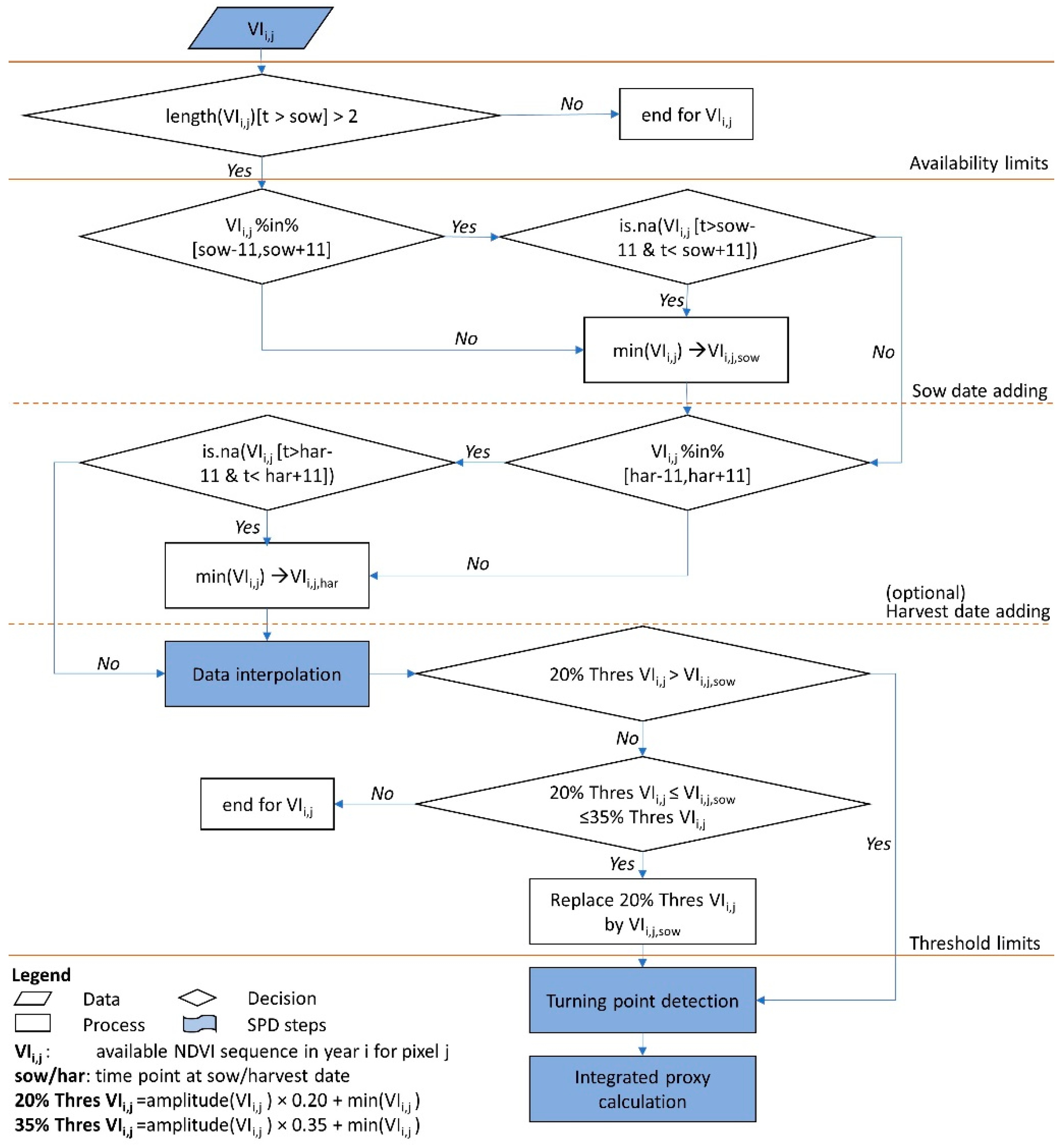
Figure 3 details the conditions for including sowing date and rainfall-based break-of-season date as additional data in the NDVI sequence before performing statistical phenology detection (SPD) using the methods outlined in Section 3.1.1. The steps are:

(1)

‘Availability limits’ excluded the pixels in the years that have less than 3 available cloud-free remote sensing observations after actual/estimated sow dates;

(2)

‘Sow date adding’ regulate the conditions to add additional information as there is no cloud-free NDVI value available in the ‘time windows’ before and after 11 days to the actual/estimated sow date. The ‘time window’ was defined as 2/3 of Landsat revisit time (16 days). We assume that there was no vegetation except bare soil across the fields on SD/BOS. As such, the spectral signature captured by remote sensing on SD/BOS was mostly made of soil reflectance. As the soil water and nutrient distribution were assumed to be inconsistent across the fields, we cannot simply give a single NDVI value to all the pixels on that day. Instead, we assumed that the NDVI value on SD/BOS was the lowest throughout the growing season for a certain pixel, and the value was set based on the original available NDVI sequence;

(3)

‘Harvest date adding’ followed the same conditions as ‘sow date adding’. Because the harvest dates across WA wheat belt were mostly based on the farmer’s own schedule rather than a certain weather pattern [34], we then made this step optional;

(4)

‘Threshold limits’ was a step for checking the rationality of the fitted curve. The 20% threshold is critical to determine the date of start of season (SOS) (see Section 3.1.1). The NDVI value on SOS date was assumed to be higher than the NDVI value on SD/BOS. However, the ‘reconstructed sequence’ contains bias due to the irregular distribution of limited available time points (Supplementary Materials File S1). In these cases, we either replace the calculated 20% threshold by SD/BOS NDVI, or exclude the pixel in a certain year, based on the comparison to the 35% limit (Figure 3).

3.1.3. Yield Estimation Using Integrated NDVI Metrics

For each of the three statistical models (SPD, +SD, and +BOS), we regressed each of the integrated NDVI metrics (POSV, iNDVI, GLAD and VLAD) against the yield for each year. For each regression model, the Akaike Information Criterion (AIC) was calculated as a measure of the goodness of fit of the model [35]. The metrics that resulted in the minimum AIC for each year were selected as the single best metric for estimating yield in that year. The results of the metrics selection process can be found in Supplementary Materials File S1.

3.1.4. The SCYM Model

The SCYM algorithm generates pixel-by-pixel grain yield estimation based on combinations of clear-sky VIs and crop simulations. The overall workflow involves three steps:

(1)

APSIM crop model simulations: The APSIM model is a process-based model that is well-adapted to systematically simulate interactions between crop and environment at a daily time step, especially in Australia. We selected seven soil types and four winter wheat cultivars, which comprise a total of twenty-eight simulations. The soil types were selected to be geographically closest to the two fields in Merredin: acid yellow sandy earth, loamy sand, duplex sandy gravel, yellow-brown shallow loamy duplex, pale sandy earth (shallow), deep sand duplex, and shallow loamy duplex. The wheat cultivars were the main cultivars planted in the two fields: Mace, Calingiri, Arrino, and Wyalkatchem. APSIM was run from 1 January 2000 to 31 December 2018. The sowing date was allowed to vary from year to year using the break of season and was assumed to occur if 15 mm of rainfall was accumulated over 3 days after 25 April, or 5 mm over 3 days after 5 June [4]. Emergence, flowering, maturity, end of grain filling dates, leaf area index (LAI) and grain yield were output by APSIM and LAI was converted to GCVI using the approach of Lobell et al. [26] and Azzari et al. [36];

(2)

Yield model calibration: The simulated GCVI data at different combinations of image dates were regressed against yield. Specifically, we divided the growing season into two, two-month periods: ‘early season’ (before 5 September) and ‘late season’. The 5 September date was calculated based on the average season of GCVI sequences. The combination set of dates were one image acquisition dates in each of the two-month windows. The general form of the regression model was (Equation (3)):

$$\mathrm{Y}={\beta }_{0d}+{\beta }_{ed}\times {\mathrm{VI}}_{ed}+{\beta }_{ld}\times {\mathrm{VI}}_{ld}+\epsilon$$

(3)

where, β = $({\beta }_{0d, }$ ${\beta }_{ed}, {\beta }_{ld})$ are the coefficients corresponding to the intercept, VI dates in early season (e) and VI dates in the late season (l), and d is one of the possible combination-sets of dates. The coefficients, β, was estimated by running the regression models using APSIM outputs and then stored in a lookup table;

(3)

Pixel by pixel yield estimation: The pre-processed Landsat 07 CGVI images in the ‘early season’ and ‘late season’ groups were composited into two sets of images preserving the maximum GCVI for each pixel, and the day of the year (DOY) for that maximum, respectively. Then, the spatial yields were estimated using the regression models, calibrated in the previous step, corresponding to the date combinations (d) for each pixel.

3.2. Model Assessment

We assessed the pixel-by-pixel error for training field J and used it to set up the thresholds to determine when additional information should be included in statistical phenology detection (methods +SD and +BOS). Identification of the single best phenological metric for yield estimation and yield regression models were also trained using data from field J.

The correlation coefficient (r) and root-mean-standard-error (RMSE) between estimated and actual yields are used to compare the performance of yield estimation models. The r and RMSE for the pixels year by year, and for the pixels in all the years, were calculated for test field M. In addition, at each pixel, we consider the absolute yield difference (tonnes/ha) in each year and r and RMSE across all years.

4. Results

4.1. Preliminary Data Exploration and SPD Model Calibration Using Training Field J

Figure 4a shows the availability of Landsat 7 imagery for field site J. The number of available images in the farmer-reported wheat season (11 ± 1 images for 191 ± 18 days) accounts for half of the images throughout a whole year (21 ± 2 images for 365 days) on average during 2003–2017. The numbers of cloud-free images in non-farming seasons are generally higher in the farming seasons, especially in years 2009, 2012 and 2017. In addition, the number of images which have the percentage of clear-sky pixels less than 50%, in farming seasons and in all the years, were 38/111 and 74/210, respectively.

Figure 4b shows the relationship between available clear-sky NDVIs and spatial yield. We found that: (1) the correlation between NDVI and yield estimation for a single image was low and variable. From 2003–2017, there were only 7 time points when the correlation between NDVIs and yield were higher than 0.5. The 7 time points were: 26 September 2003 (r = 0.51), 03 July 2013 (r = 0.55), 04 August 2013 (r = 0.62), 20 August 2013 (r = 0.58), 25 July 2015 (r = 0.55), and 10 August 2015 (r = 0.55) in sequence. The months range from early July to late September. Accordingly, in all years except 2003, 2013 and 2015, there was no single NDVI image that had the ability to explain more than 50% of yield variation regardless of the percentage of available clear-sky pixels; (2) the correlations were varying throughout and across the farmer-reported wheat seasons. In the typical years of 2007, 2013, 2016, and 2017, the correlation coefficients followed a seasonal pattern where they firstly increased and then decreased as the season progressed. However, in the rest of the years that wheat was planted in field J, the patterns were irregular. In 2009, none of the available NDVI images in the farming season had correlation coefficients with a yield higher than 0.2. In addition, the correlation coefficient on 28 October 2009 was −0.25, while the available clear-sky pixels accounts for 1% of the total interested pixels.

Supervised pixel-by-pixel error assessments for field J (Supplementary Materials File S1) indicated that the rationality of fitted curve and detected turning points is greatly affected by the number of available data points and their positions in a sequence. The bias is foreseeable for pixels where there were few clear-sky remote sensing observations, or where the available data were irregularly located in the sequences. Therefore, we set up rules to conditionally include additional information about sowing date (SD) or break of season (BOS) date before fitting the times series curves. The purpose of adding SD/BOS was to control the shape of the curve and to simultaneously assess the curve shape. We then identified the single best phenological metric for yield estimation and yield regression models using data from field J, see

Table 3. For statistical phenology detection (SPD), statistical phenology detection incorporates sowing date (+SD) and statistical phenology detection incorporates break of season (+BOS), the integrated NDVI metrics with minimum AIC for yield estimation, estimated yield model parameters (a,b) and accuracy statistics (r, AIC, RMSE) from 2003 to 2017.

Model	Parameters	Year
		2003	2004	2006	2007	2009	2012	2013	2015	2016	2017
SPD	Proxy	POSV	POSV	GLAD	VLAD	POSV	POSV	VLAD	iNDVI	POSV	GLAD
	a	1.176	0.918	0.043	0.031	0.273	0.594	0.078	0.043	0.803	0.065
	b	1.272	0.815	0.738	0.119	1.056	0.184	0.660	0.724	1.255	1.089
	r	0.253	0.276	0.350	0.401	0.073	0.148	0.596	0.520	0.249	0.374
	AIC	3039	162	−597	−1902	1249	−666	2131	1290	944	803
	RMSE	0.397	0.249	0.219	0.174	0.297	0.216	0.346	0.301	0.284	0.277
‘+SD’	Proxy	POSV	POSV	VLAD	VLAD	POSV	POSV	VLAD	VLAD	POSV	GLAD
	a	1.167	0.917	0.035	0.029	0.272	0.700	0.077	0.079	0.842	0.065
	b	1.269	0.815	0.765	0.140	1.057	0.142	0.680	0.735	1.234	1.093
	r	0.249	0.276	0.326	0.403	0.073	0.156	0.592	0.541	0.258	0.376
	AIC	3046	162	−649	−1895	1249	−550	2144	1197	930	792
	RMSE	0.397	0.249	0.216	0.174	0.298	0.218	0.347	0.296	0.283	0.277
‘+BOS’	Proxy	POSV	POSV	iNDVI	VLAD	POSV	POSV	VLAD	VLAD	POSV	GLAD
	a	1.199	0.918	0.022	0.030	0.293	0.602	0.078	0.080	0.781	0.065
	b	1.248	0.814	0.685	0.134	1.044	0.181	0.661	0.741	1.270	1.081
	r	0.262	0.276	0.362	0.402	0.077	0.150	0.595	0.545	0.241	0.374
	AIC	3024	162	−628	−1895	1211	−670	2135	1181	930	803
	RMSE	0.396	0.249	0.218	0.174	0.296	0.216	0.346	0.295	0.283	0.277

and Supplementary Materials File S1.

4.2. Incorporating Additional Information into Statistical Phenology Detection

We applied the conditional settings to include additional information in SPD and the yield estimation models trained on field J to test field M. Comparison of year-by-year yield estimates and actual yields for field M using different models can be found in Supplementary Materials File S2.

Table 4. A summary of the number of pixels processed with conditional setting in phenology detection incorporates sowing date (+SD) and break of season (+BOS) for testing field M from 2003 to 2017.

Conditional Setting	Model	Year (Count of Pixels)
		2003	2004	2007	2009	2012	2013	2016	2017
Availability limits exceed	+SD/BOS	6	26	42	19	24	14	87	33
>35% threshold exceed	+SD	1	0	6	6	10	2	13	17
	+BOS	33	0	6	10	7	0	85	0
Have option to add sow date	+SD	1828	1808	152	0	62	144	100	0
	+BOS	1828	60	152	0	0	1820	111	1801
Have option to add harvest date	+SD	54	0	0	0	1810	1471	0	170
Threshold value switch	+SD	0	0	91	36	34	13	143	106
	+BOS	51	3	71	86	24	0	706	0
Estimated SOS corrected	+SD	675	41	79	36	45	11	243	98
	+BOS	675	2	27	36	7	2	71	45
Total pixels	Actual yield	1828	1808	1792	1815	1810	1820	1747	1801
	SCYM	1731	1808	1792	1815	1810	1820	1747	1801

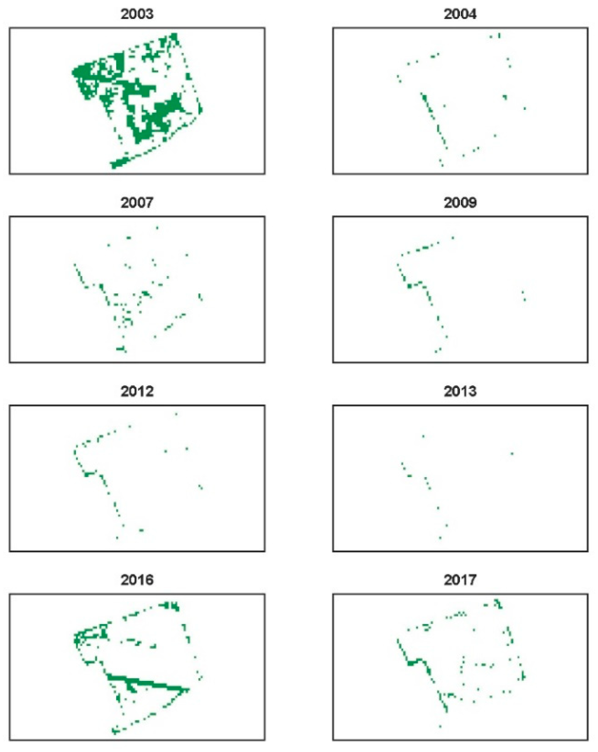
‘Conditional setting’ is described in Figure 3. ‘Estimated SOS changed’ refer to the pixels where the SOS date estimated using statistical phenology detection (SPD) is earlier than the farmer-reported sowing date but has been corrected to be later than the farmer-reported sowing date in the +SD or +BOS models.

shows that varying number of pixels were processed in all the steps to include SD/BOS in SPD each year. The number of pixels where the SOS date was corrected from the SPD model accounts for less than half of the total number of the pixels where the conditions were met in both +SD and +BOS models. Year 2003 had the highest proportion of pixels where the SOS date was corrected (n = 675), which accounted for one-third of the tested pixels. 2013 only had their estimated SOS corrected by either +SD or +BOS for less than 1% of the total considered pixels. In addition, the +SD model resulted in more pixel corrections on estimated SOS than the +BOS model in all the wheat planting years.

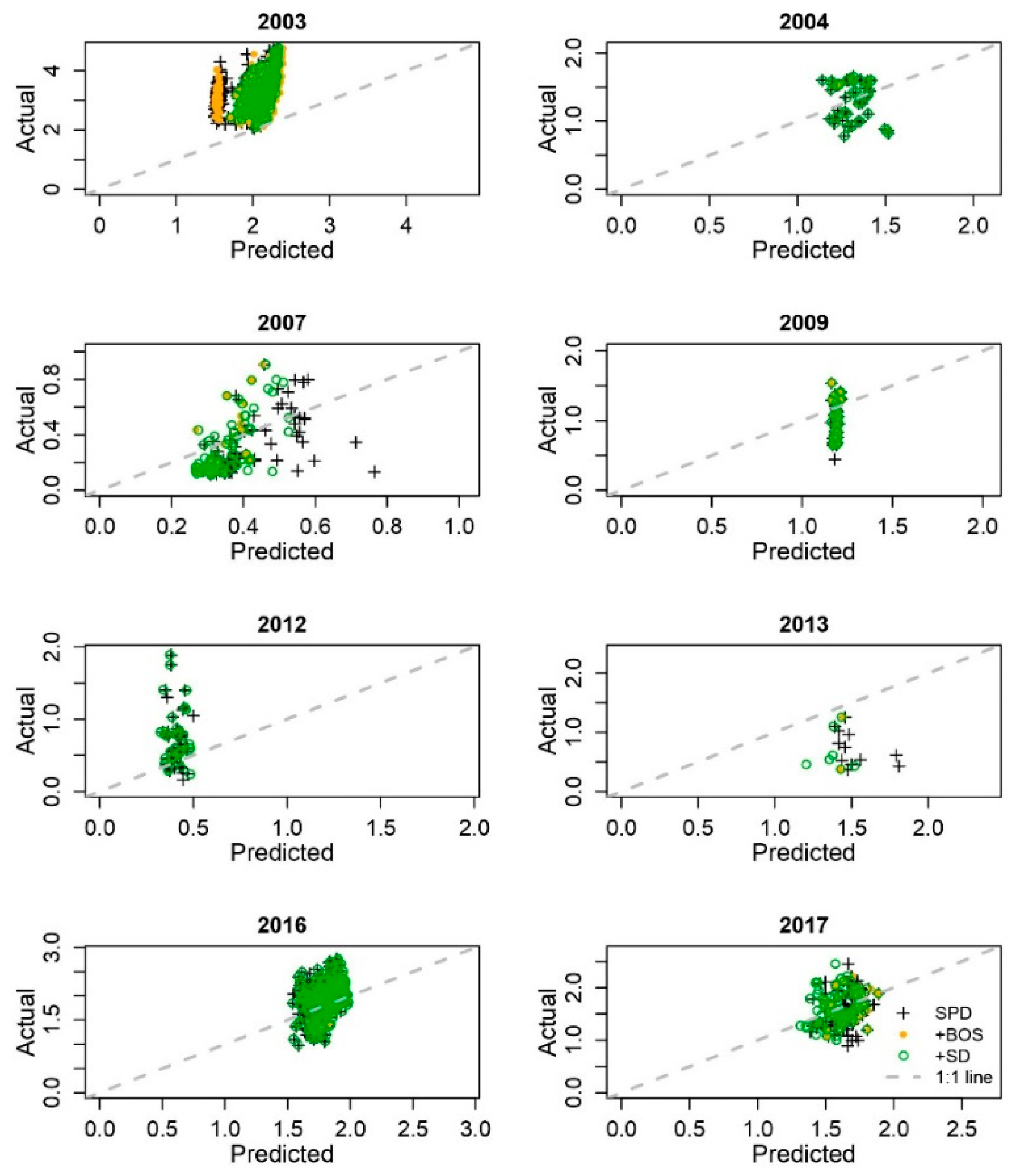
Figure 5 shows that the pixels that had their estimated SOS date corrected by the +SD model are mostly located in the margin area of the field, except in 2003. Meanwhile, Figure 6 gives the correlations between the actual and estimated yields at those pixels where the estimated SOS date was corrected from SPD to either +SD or +BOS. The estimated yields using either +SD or +BOS have less variation and a narrower range than the estimated yields using SPD, especially in years 2003, 2007, and 2013. When compared to the 1:1 line, the estimated yields using +SD/BOS tend to cluster to the mean actual yield each year, especially in 2003.

4.3. Yield Predictors Using Statistical Phenology Detection Compared to SCYM

We compared yield estimation using integrated NDVI metrics derived from the three statistical phenology detection models (SPD, +BOS, or +SD) and the SCYM-selected GCVI predictors for both overall and year-by-year assessments in field M.

Overall, all four models perform yield estimation well. The SCYM model had a lower correlation coefficient (r) and higher root mean square error (RMSE) than the SPD/+BOS/+SD models (

Table 5. Annual accuracy statistics comparing actual yield and estimated yields using the four models: Statistical phenology detection (SPD), statistical phenology detection incorporates sowing date (+SD), statistical phenology detection incorporates break of season (+BOS) and scalable crop yield mapper (SCYM). Accuracy statistics reported are correlation coefficient (r) and root mean square error (RMSE).

Year	Accuracy statistic	SPD	+BOS	+SD	SCYM
2003	r	0.38	0.41	0.59	0.58
	RMSE	1.27	1.23	1.23	0.92
2004	r	0.34	0.34	0.35	0.36
	RMSE	0.25	0.25	0.25	0.49
2007	r	0.76	0.78	0.79	0.51
	RMSE	0.21	0.21	0.21	0.57
2009	r	0.53	0.51	0.51	0.22
	RMSE	0.33	0.33	0.33	0.66
2012	r	0.50	0.50	0.50	0.34
	RMSE	0.92	0.92	0.90	0.38
2013	r	0.59	0.60	0.53	0.38
	RMSE	0.34	0.34	0.31	0.40
2016	r	0.23	0.16	0.21	0.15
	RMSE	0.41	0.41	0.40	0.55
2017	r	0.59	0.60	0.57	0.37
	RMSE	0.23	0.23	0.23	0.80
Mean	r	0.80	0.80	0.81	0.70
	RMSE	0.61	0.60	0.56	0.62

Note: Mean calculates r and RMSE between observed and estimated yield for all pixels across all years (see Section 3.2).

). In each year, the correlations between estimated and actual yield vary year-by-year and proxy-by-proxy (Table 5). The range of r and RMSE for 8 years of per-pixel yield estimation are: 0.15 (by SCYM in 2016) < r < 0.79 (by +SD in 2007), 0.21 tonnes/ha (by SPD/+BOS/+SD in 2007) < RMSE < 1.27 tonnes/ha (by SPD in 2003) (Table 5). SCYM estimates have higher r with yield than the statistical model estimates in only year 2004. However, the SCYM produced higher RMSE in 2004. In 2003 and 2012, the three statistical models have higher RMSE. In addition, SPD, +BOS, and +SD performed similarly in each single year. Although the order of the three statistical models based on r vary year by year, the RMSE produced by +BOS/+SD were always equal or smaller than by SPD.

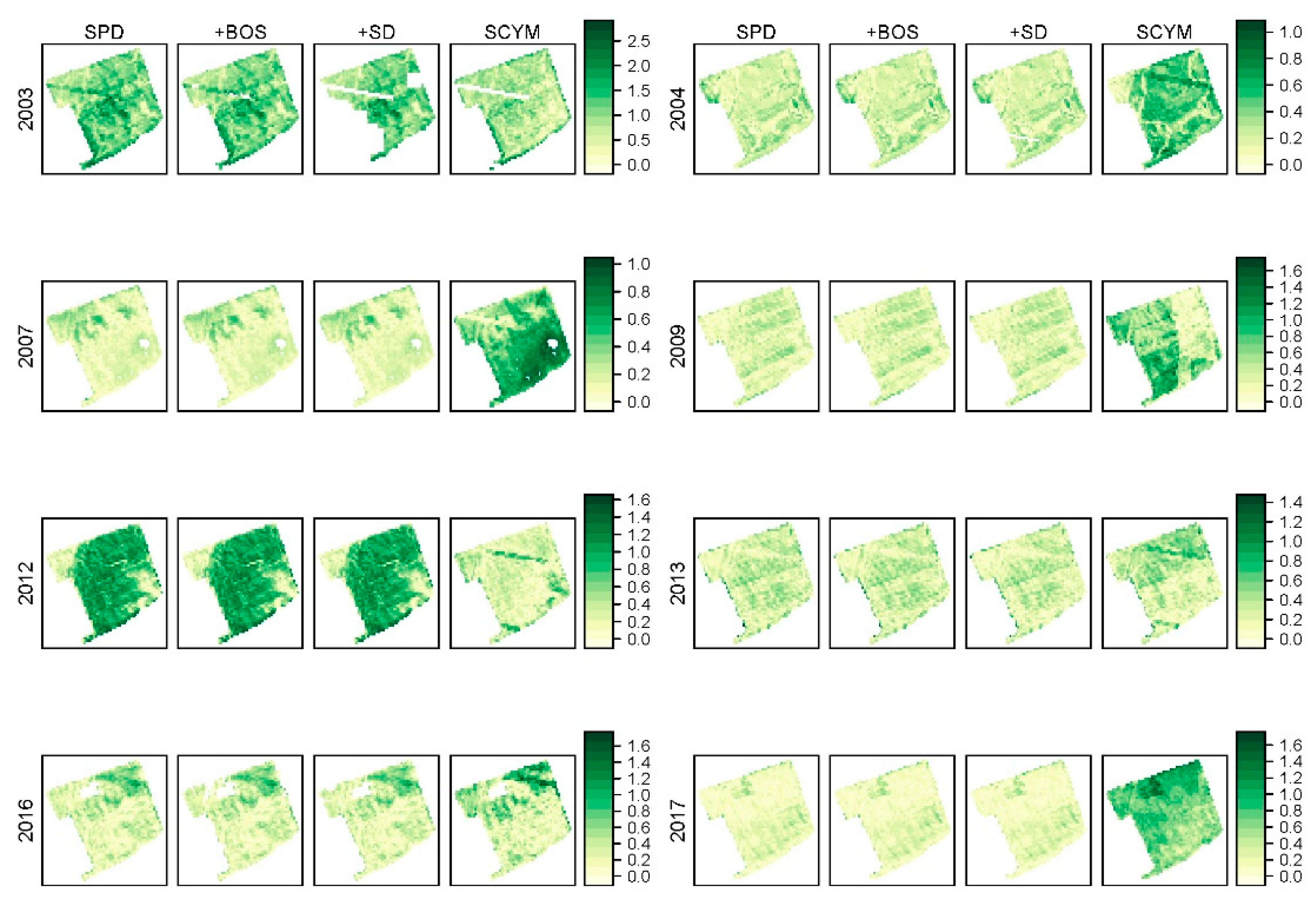
We produced estimated yield maps for field M (Supplementary Materials File S2) and the corresponding absolute yield difference between actual and estimated (Figure 7). The estimates using integrated NDVI metrics from statistical phenology detection models (using SPD, +BOS, or +SD) had overall lower absolute yield difference with actual yield (0.44 tonnes/ha using SPD, 0.44 tonnes/ha using +BOS, and 0.43 tonnes/ha using +SD) than the SCYM estimates (0.53 tonnes/ha), except for year 2003 and 2012. Spatially, the pixels with error are more likely to be located in the field edges and tractor path lines within the paddock (darker green colours in Figure 7).

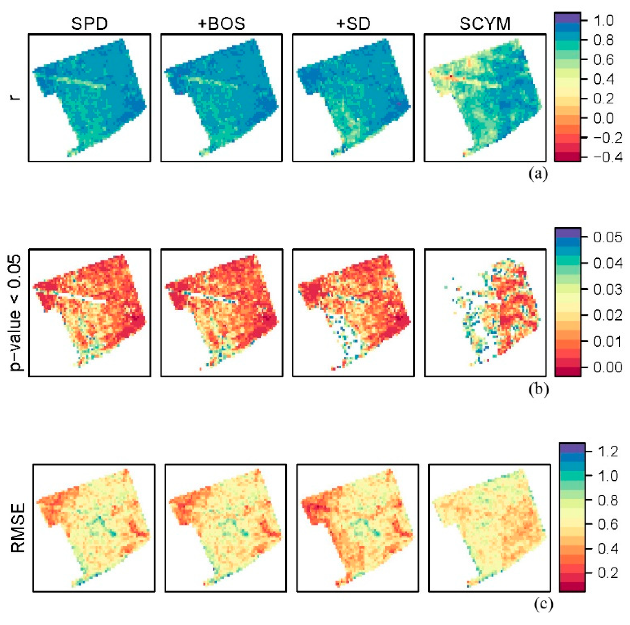
Figure 8 shows the correlations between actual and estimated yields at pixel level for the years which reflects the temporal consistency of the estimates within-field. Compared to SPD and +BOS, the +SD model improved r in the field edge area and the lines covered by Landsat 7 failure scanner. Compared to the statistical phenology detection models, SCYM had overall lower r, higher RMSE, and fewer pixels with significant yearly correlation (p-value < 0.05). The high RMSE (>1.0 tonnes/ha) are mostly located in the field edge area using either SPD or SCYM. The +SD model eased this situation and had fewer edging pixels with RMSE > 1.0 tonnes/ha.

5. Discussion

This study investigated the use of sequences of Landsat NDVI for estimating wheat yield in fields in Western Australia (WA). Preliminary investigation of the Landsat 7 NDVI and yield at training field J showed that the relationships between integrated NDVI metrics and yield varied by year and location and was heavily influenced by missing data in the NDVI time sequences. This finding agrees with previous studies [37,38,39] and shows that, due to seasonal and spatial variability, any one metric has limited ability for yield estimation within a field. Waldner et al. [40] quantified the positive relationship between temporal resolution of VI sequences and accuracy of empirical estimation on grain yield based on crop modelling. We also found that the position of missing values in a VI sequence matters when the sequence is integrated to estimate yield in fields.

Cai et al. [41] concluded that there is no single method for reconstruction of NDVI time sequences that always perform better than others, unless the smoothing parameters are locally calibrated. In this study, we calibrated optimal smoothing parameters for the statistical phenological detection (SPD) model using local data for training field J (Supplementary Materials File S1). The SPD model was still affected by missing data in the NDVI time sequence, particularly when data were missing in the early to middle parts of the growing season. We hypothesised that conditionally adding sow dates (SD) or break of season (BOS) dates would improve the accuracy of yield estimation using integrated NDVI metrics derived from SPD. We tested this hypothesis by applying smoothing parameters and yield estimation models trained on field J to test field M but found it was true for only a small proportion of pixels each year. These pixels were mostly located in the edges of the field and the inclusion of SD resulted in slightly lower RMSE in yield estimation compared to the estimates from SPD (Table 5). While the simple constraint of ensuring that SD/BOS occurred before start of season (SOS) helped control the shape of the fitted phenological curves, it did not ensure higher correlation coefficients (r) between estimated and actual yields for pixels within-field each year.

The scalable crop yield mapper (SCYM) has been shown to have potential for within-field yield estimation [20,26,36]. It calculates an empirical relationship between ‘greenness’ proxy GCVI at particular times with yield simulated using a process-based crop growth model. However, SCYM uses GCVI once or twice only and does not consider the progress of crop growth throughout the growing season. We compared the SCYM model with the use of integrated NDVI metrics derived from SPD (with and without the addition of SD or BOS). We used a set of APSIM simulations generated for all possible farming scenarios in our study area to derive the SCYM relationship between GCVI and yield. We found that SCYM estimated yield had lower r and higher RMSE compared to actual yield than the SPD/+SD/+BOS estimates in most years. In addition, SCYM performance was variable across years and spatially within the test field. In-situ calibration datasets are needed for its further application in precision agriculture [42], especially in locations with a Mediterranean winter.

Our study found year-location-proxy specific relationships between integrated NDVI metrics and within-field yield that may have been caused by a number of reasons. Intra-seasonal rainfall distribution may influence the relationship between NDVI and plant biomass [43]. Micro-climates in field caused by waterlogging, shelterbelt-effect and topography [44] may go undetected by satellite sensors. In addition, errors may arise from atmospheric correction routines [45] applied to remotely sensed data or from interpolation of dense yield monitor data to a grid of 30 × 30 m [46,47], all of which may propagate through to the yield estimates.

Crop yield is a result of interactions from crop genotype (G), farm management (M), and environmental factors (E). Integrated NDVI metrics obtained from sequences of remotely-sensed NDVI capture part of the G×M×E effects on yield [40]. However, there are many G×M×E effects that cannot be measured from space (e.g., evapotranspiration, ratio of aboveground biomass to grain yield, grain quality and crop diseases) that remain sources of uncertainty when estimating yield using remote sensing. Some of this uncertainty might be resolved with the use of ancillary datasets, such as finer resolution remote sensing observations, soil maps, and continuous climate records [48,49,50,51]. This would require more complex yield estimation models than the simple linear regressions used in this study. Machine learning (e.g., random forests or deep learning approaches) has great potential for automatic selection of appropriate integrated NDVI metrics and ancillary data for within-field yield estimation in different years and locations. For example, Kamir et al. [33] used nine different machine learning algorithms for yield estimation from remotely sensed NDVI and climate data at 250 m resolution, but their methods are yet to be tested at a resolution that would allow for application to precision agriculture. Integration of Sentinel-2 imagery is also expected as it accumulates sufficient observations. We anticipate that future works will leverage machine learning approaches and consider additional data to improve the ability of yield estimation using sequences of remote sensing NDVI.

6. Conclusions

Incorporating farmer-reported sow dates (SD) in statistical phenological detection (SPD) marginally improved yield estimation from derived integrated NDVI metrics overall. But the inclusion of break of season (BOS) information did not show obvious improvement. In addition, the inclusion of the additional SD/BOS information corrected detection of start of season (SOS) for some pixels that were mostly located in the field edges. This had little effect on the accuracy of within-field yield estimation, but estimated yields had higher spatial and temporal consistency with the actual yield. Yield estimation using integrated NDVI metrics derived from SPD was more accurate than yield estimation using the Scalable Yield Mapper (SCYM) model. However, the accuracy of estimated within-field yield using any of the tested methods was limited and variable because of: (1) the varying availability of NDVI in the time-sequences for pixels; (2) the variable environment within the field; (3) variable seasonal weather conditions year-by-year; and (4) space and time dependency of the relationship between satellite measurements and yield. We conclude that sequences of Landsat NDVI have the potential to estimation wheat yield variation in fields in Western Australia, but they need to be incorporated with additional sources of data to distinguish between different years and locations.

References

- Department of Primary Industries and Regional Development. Western Australian Grains Industry. Available online: https://agric.wa.gov.au/n/2072 (accessed on 1 March 2021).
- Evans, F.H.; Guthrie, M.M.; Foster, I. Accuracy of six years of operational statistical seasonal forecasts of rainfall in Western Australia (2013 to 2018). Atmos. Res. 2020, 233, 104697. [Google Scholar] [CrossRef]
- McBratney, A.; Whelan, B.; Ancev, T.; Bouma, J. Future Directions of Precision Agriculture. Precis. Agric. 2005, 6, 7–23. [Google Scholar] [CrossRef]
- Asseng, S.; Turner, N.C.; Keating, B.A. Analysis of water- and nitrogen-use efficiency of wheat in a Mediterranean climate. Plant Soil 2001, 233, 127–143. [Google Scholar] [CrossRef]
- Belward, A.S.; Skøien, J.O. Who launched what, when and why; trends in global land-cover observation capacity from civilian earth observation satellites. ISPRS J. Photogramm. Remote Sens. 2015, 103, 115–128. [Google Scholar] [CrossRef]
- Wulder, M.A.; White, J.C.; Loveland, T.R.; Woodcock, C.E.; Belward, A.S.; Cohen, W.B.; Fosnight, E.A.; Shaw, J.; Masek, J.G.; Roy, D.P. The global Landsat archive: Status, consolidation, and direction. Remote Sens. Environ. 2016, 185, 271–283. [Google Scholar] [CrossRef] [Green Version]
- Rouse, J.W.; Haas, R.H.; Schell, J.A.; Deering, D.W.; Harlan, J.C. Monitoring the Vernal Advancement and Retrogradation (Green Wave Effect) of Natural Vegetation; NASA/GSFC Type III Final Report: Greenbelt, MD, USA, 1974; p. 371. [Google Scholar]
- Wall, L.; Larocque, D.; Léger, P.M. The early explanatory power of NDVI in crop yield modelling. Int. J. Remote Sens. 2008, 29, 2211–2225. [Google Scholar] [CrossRef]
- Zhang, X.; Friedl, M.A.; Schaaf, C.B.; Strahler, A.H.; Hodges, J.C.; Gao, F.; Reed, B.C.; Huete, A. Monitoring vegetation phenology using MODIS. Remote Sens. Environ. 2003, 84, 471–475. [Google Scholar] [CrossRef]
- Broich, M.; Huete, A.; Paget, M.; Ma, X.; Tulbure, M.; Coupe, N.R.; Evans, B.; Beringer, J.; Devadas, R.; Davies, K. A spatially explicit land surface phenology data product for science, monitoring and natural resources management applications. Environ. Model. Softw. 2015, 64, 191–204. [Google Scholar] [CrossRef]
- Araya, S.; Ostendorf, B.; Lyle, G.; Lewis, M. CropPhenology: An R package for extracting crop phenology from time series remotely sensed vegetation index imagery. Ecol. Inform. 2018, 46, 45–56. [Google Scholar] [CrossRef]
- Shen, J.; Huete, A.; Tran, N.N.; Devadas, R.; Ma, X.; Eamus, D.; Yu, Q. Diverse sensitivity of winter crops over the growing season to climate and land surface temperature across the rainfed cropland-belt of eastern Australia. Agric. Ecosyst. Environ. 2018, 254, 99–110. [Google Scholar] [CrossRef]
- Zeng, L.; Wardlow, B.D.; Xiang, D.; Hu, S.; Li, D. A review of vegetation phenological metrics extraction using time-series, multispectral satellite data. Remote Sens. Environ. 2020, 237, 111511. [Google Scholar] [CrossRef]
- Lai, Y.R.; Pringle, M.J.; Kopittke, P.M.; Menzies, N.W.; Orton, T.G.; Dang, Y.P. An empirical model for prediction of wheat yield, using time-integrated Landsat NDVI. Int. J. Appl. Earth Obs. Geoinf. 2018, 72, 99–108. [Google Scholar] [CrossRef]
- Becker-Reshef, I.; Vermote, E.; Lindeman, M.; Justice, C. A generalized regression-based model for forecasting winter wheat yields in Kansas and Ukraine using MODIS data. Remote Sens. Environ. 2010, 114, 1312–1323. [Google Scholar] [CrossRef]
- Bolton, D.K.; Friedl, M.A. Forecasting crop yield using remotely sensed vegetation indices and crop phenology metrics. Agric. For. Meteorol. 2013, 173, 74–84. [Google Scholar] [CrossRef]
- Sakamoto, T.; Gitelson, A.A.; Arkebauer, T.J. Near real-time prediction of U.S. corn yields based on time-series MODIS data. Remote Sens. Environ. 2014, 147, 219–231. [Google Scholar] [CrossRef]
- Roy, D.P.; Yan, L. Robust Landsat-based crop time series modelling. Remote Sens. Environ. 2020, 238, 110810. [Google Scholar] [CrossRef]
- Whitcraft, A.K.; Vermote, E.F.; Becker-Reshef, I.; Justice, C.O. Cloud cover throughout the agricultural growing season: Impacts on passive optical earth observations. Remote Sens. Environ. 2015, 156, 438–447. [Google Scholar] [CrossRef]
- Weiss, M.; Jacob, F.; Duveiller, G. Remote sensing for agricultural applications: A meta-review. Remote Sens. Environ. 2020, 236, 111402. [Google Scholar] [CrossRef]
- Bolton, D.K.; Gray, J.M.; Melaas, E.K.; Moon, M.; Eklundh, L.; Friedl, M.A. Continental-scale land surface phenology from harmonized Landsat 8 and Sentinel-2 imagery. Remote Sens. Environ. 2020, 240, 111685. [Google Scholar] [CrossRef]
- Gao, F.; Anderson, M.C.; Zhang, X.; Yang, Z.; Alfieri, J.G.; Kustas, W.P.; Mueller, R.; Johnson, D.M.; Prueger, J.H. Toward mapping crop progress at field scales through fusion of Landsat and MODIS imagery. Remote Sens. Environ. 2017, 188, 9–25. [Google Scholar] [CrossRef] [Green Version]
- He, M.; Kimball, J.S.; Maneta, M.P.; Maxwell, B.D.; Moreno, A.; Beguería, S.; Wu, X. Regional Crop Gross Primary Productivity and Yield Estimation Using Fused Landsat-MODIS Data. Remote Sens. 2018, 10, 372. [Google Scholar] [CrossRef] [Green Version]
- Meng, L.; Liu, H.; Zhang, X.; Ren, C.; Ustin, S.; Qiu, Z.; Xu, M.; Guo, D. Assessment of the effectiveness of spatiotemporal fusion of multi-source satellite images for cotton yield estimation. Comput. Electron. Agric. 2019, 162, 44–52. [Google Scholar] [CrossRef]
- Chen, Y.; McVicar, T.R.; Donohue, R.J.; Garg, N.; Waldner, F.; Ota, N.; Li, L.; Lawes, R. To Blend or Not to Blend? A Framework for Nationwide Landsat–MODIS Data Selection for Crop Yield Prediction. Remote Sens. 2020, 12, 1653. [Google Scholar] [CrossRef]
- Lobell, D.B.; Thau, D.; Seifert, C.; Engle, E.; Little, B. A scalable satellite-based crop yield mapper. Remote Sens. Environ. 2015, 164, 324–333. [Google Scholar] [CrossRef]
- Chen, K.; O’Leary, R.A.; Evans, F.H. A simple and parsimonious generalised additive model for predicting wheat yield in a decision support tool. Agric. Syst. 2019, 173, 140–150. [Google Scholar] [CrossRef]
- Pebesma, E.; Heuvelink, G. Spatio-temporal interpolation using gstat. RFID J. 2016, 8, 204–218. [Google Scholar]
- Pebesma, E.J. Multivariable geostatistics in S: The gstat package. Comput. Geosci. 2004, 30, 683–691. [Google Scholar] [CrossRef]
- Moritz, S.; Bartz-Beielstein, T. imputeTS: Time series missing value imputation in R. R J. 2017, 9, 207–218. [Google Scholar] [CrossRef] [Green Version]
- Stineman, R.W. A consistently well-behaved method of interpolation. Creat. Comput. 1980, 6, 54–57. [Google Scholar]
- Guerschman, J.P.; Hill, M.J.; Renzullo, L.J.; Barrett, D.J.; Marks, A.S.; Botha, E.J. Estimating fractional cover of photosynthetic vegetation, non-photosynthetic vegetation and bare soil in the Australian tropical savanna region upscaling the EO-1 Hyperion and MODIS sensors. Remote Sens. Environ. 2009, 113, 928–945. [Google Scholar] [CrossRef]
- Kamir, E.; Waldner, F.; Hochman, Z. Estimating wheat yields in Australia using climate records, satellite image time series and machine learning methods. ISPRS J. Photogramm. Remote Sens. 2020, 160, 124–135. [Google Scholar] [CrossRef]
- Smith, R.; Adams, J.; Stephens, D.; Hick, P. Forecasting wheat yield in a Mediterranean-type environment from the NOAA satellite. Aust. J. Agric. Res. 1995, 46, 113–125. [Google Scholar] [CrossRef]
- AKAIKE, H. Maximum likelihood identification of Gaussian autoregressive moving average models. Biometrika 1973, 60, 255–265. [Google Scholar] [CrossRef]
- Azzari, G.; Jain, M.; Lobell, D.B. Towards fine resolution global maps of crop yields: Testing multiple methods and satellites in three countries. Remote Sens. Environ. 2017, 202, 129–141. [Google Scholar] [CrossRef]
- Younes, N.; Joyce, K.E.; Maier, S.W. All models of satellite-derived phenology are wrong, but some are useful: A case study from northern Australia. Int. J. Appl. Earth Obs. Geoinf. 2021, 97, 102285. [Google Scholar] [CrossRef]
- Colaço, A.F.; Bramley, R.G.V. Site–Year Characteristics Have a Critical Impact on Crop Sensor Calibrations for Nitrogen Recommendations. Agron. J. 2019, 111, 2047–2059. [Google Scholar] [CrossRef]
- Wang, B.; Feng, P.; Liu, D.L.; O’Leary, G.J.; Macadam, I.; Waters, C.; Asseng, S.; Cowie, A.; Jiang, T.; Xiao, D.; et al. Sources of uncertainty for wheat yield projections under future climate are site-specific. Nat. Food 2020. [Google Scholar] [CrossRef]
- Waldner, F.; Horan, H.; Chen, Y.; Hochman, Z. High temporal resolution of leaf area data improves empirical estimation of grain yield. Sci. Rep. 2019, 9, 15714. [Google Scholar] [CrossRef] [Green Version]
- Cai, Z.; Jönsson, P.; Jin, H.; Eklundh, L. Performance of Smoothing Methods for Reconstructing NDVI Time-Series and Estimating Vegetation Phenology from MODIS Data. Remote Sens. 2017, 9, 1271. [Google Scholar] [CrossRef] [Green Version]
- Jeffries, G.R.; Griffin, T.S.; Fleisher, D.H.; Naumova, E.N.; Koch, M.; Wardlow, B.D. Mapping sub-field maize yields in Nebraska, USA by combining remote sensing imagery, crop simulation models, and machine learning. Precis. Agric. 2020, 21, 678–694. [Google Scholar] [CrossRef]
- Mbow, C.; Fensholt, R.; Rasmussen, K.; Diop, D. Can vegetation productivity be derived from greenness in a semi-arid environment? Evidence from ground-based measurements. J. Arid Environ. 2013, 97, 56–65. [Google Scholar] [CrossRef]
- Pryor, D.; Nadler, A. Examining micro-climate effects in field crop production. In Proceedings of the 7th Annual Manitoba Agronomists Conference, Winnipeg, MB, Canada, December 2008. [Google Scholar]
- Claverie, M.; Vermote, E.F.; Franch, B.; Masek, J.G. Evaluation of the Landsat-5 TM and Landsat-7 ETM+ surface reflectance products. Remote Sens. Environ. 2015, 169, 390–403. [Google Scholar] [CrossRef]
- Simbahan, G.C.; Dobermann, A.; Ping, J.L. Screening Yield Monitor Data Improves Grain Yield Maps. Agron. J. 2004, 96, 1091–1102. [Google Scholar] [CrossRef]
- Gaso, D.V.; Berger, A.G.; Ciganda, V.S. Predicting wheat grain yield and spatial variability at field scale using a simple regression or a crop model in conjunction with Landsat images. Comput. Electron. Agric. 2019, 159, 75–83. [Google Scholar] [CrossRef]
- Whitcraft, A.K.; Becker-Reshef, I.; Killough, B.D.; Justice, C.O. Meeting Earth Observation Requirements for Global Agricultural Monitoring: An Evaluation of the Revisit Capabilities of Current and Planned Moderate Resolution Optical Earth Observing Missions. Remote Sens. 2015, 7, 1482–1503. [Google Scholar] [CrossRef] [Green Version]
- Duncan, J.; Dash, J.; Atkinson, P. The potential of satellite-observed crop phenology to enhance yield gap assessments in smallholder landscapes. Front. Environ. Sci. 2015, 3, 56. [Google Scholar] [CrossRef] [Green Version]
- Zhao, H.; Yang, Z.; Di, L.; Pei, Z. Evaluation of Temporal Resolution Effect in Remote Sensing Based Crop Phenology Detection Studies; Springer: Berlin/Heidelberg, Germany, 2012; pp. 135–150. [Google Scholar]
- Fritz, S.; See, L.; Bayas, J.C.L.; Waldner, F.; Jacques, D.; Becker-Reshef, I.; Whitcraft, A.; Baruth, B.; Bonifacio, R.; Crutchfield, J.; et al. A comparison of global agricultural monitoring systems and current gaps. Agric. Syst. 2019, 168, 258–272. [Google Scholar] [CrossRef]
Figure 1.
The study area: (a) The 10-year mean NDVI in August in Western Australia (WA) and study area location for Merredin (MODIS Terra, 2007–2016); (b) General growing season (Aril to November) rainfall distribution in WA (Australian Bureau of Meteorology, 1961–1990); (c) NDVI derived from Landsat 08 OLI in Merredin (21 September 2016) and location of the training field J (red box) and testing field M (blue box); (d) Maximum wheat yield across the two fields from 2003–2017.
Figure 2.
Examples for field J in year 2015 of the statistical phenology detection model (SPD): (a) for field average, and (b) for a pixel. The green solid line shows the ‘reconstructed daily’ NDVI sequence. The black dashed line shows the fitted polynomial curve. The grey horizontal line shows the 20% threshold of the daily NDVI amplitude used to identify the start of season (SOS) and end of season (EOS) dates. POSV, iNDVI, VLAD, and GLAD are integrated NDVI metrics that measure different parts of the area under the ‘reconstructed daily’ curve.
Figure 3.
The workflow to conditionally include SD/BOS NDVI in statistical curve fitting. The brown horizontal lines divide the workflow into four sections: availability limits, sow date adding, harvest date adding (optional, dashed line), and threshold limits. ‘Sow date’ refers to either actual sow date (+SD) or rainfall-based break of season date (+BOS).
Figure 4.
The spatial (y-axis) and temporal (x-axis) availability of Landsat 7 images (a) and the general correlation between clear-sky NDVIs and the corresponding annual yields (b) for site J. The red/blue colours of the dots indicate the image acquisitions dates were in the farmer-reported wheat seasons (GS)/non-farming seasons (NonGS). The farmer-reported wheat seasons were defined using the farmer-provided sowing and harvest dates; The bar heights in (a) indicate the percentage of clear-sky pixels in each year; the positive correlation (r) was statistically significant when it is greater than its corresponding ‘r Critical’ (green lines in panel (b)).
Figure 5.
The pixels where the conditions were met to include sowing date (+SD) in the statistical phenological detection (SPD) and had start of season (SOS) date corrected for the testing field M.
Figure 6.
Scatterplots of actual and estimated yield for the pixels which had their estimated SOS date corrected from SPD to either +BOS or +SD.
Figure 7.
The absolute yield difference (tonnes/ha) between actual and estimated using each of the four models: statistical phenology detection (SPD), statistical phenology detection incorporates break of season (+BOS), statistical phenology detection incorporates sowing date (+SD), and scalable crop yield mapper (SCYM).
Figure 8.
For field M, the correlation between actual and estimated yields at each pixel for all the years using each of the four models: Statistical phenology detection (SPD), statistical phenology detection incorporates sowing date (+SD), statistical phenology detection incorporates break of season (+BOS) and scalable crop yield mapper (SCYM). (a) r; (b) p-value < 0.05; (c) RMSE.