Can Agricultural Management Induced Changes in Soil Organic Carbon Be Detected Using Mid-Infrared Spectroscopy?

Abstract

A major limitation to building credible soil carbon sequestration programs is the cost of measuring soil carbon change. Diffuse reflectance spectroscopy (DRS) is considered a viable low-cost alternative to traditional laboratory analysis of soil organic carbon (SOC). While numerous studies have shown that DRS can produce accurate and precise estimates of SOC across landscapes, whether DRS can detect subtle management induced changes in SOC at a given site has not been resolved. Here, we leverage archived soil samples from seven long-term research trials in the U.S. to test this question using mid infrared (MIR) spectroscopy coupled with the USDA-NRCS Kellogg Soil Survey Laboratory MIR spectral library. Overall, MIR-based estimates of SOC%, with samples scanned on a secondary instrument, were excellent with the root mean square error ranging from 0.10 to 0.33% across the seven sites. In all but two instances, the same statistically significant (p < 0.10) management effect was found using both the lab-based SOC% and MIR estimated SOC% data. Despite some additional uncertainty, primarily in the form of bias, these results suggest that large existing MIR spectral libraries can be operationalized in other laboratories for successful carbon monitoring.

1. Introduction

There is substantial political and scientific momentum to formally include soil carbon management as a climate mitigation strategy through various agricultural policies and carbon markets [1]. Some programs, such as the Australian Emissions Reduction Fund [2] and third-party carbon registries have already begun issuing carbon credits to farmers. However, a major barrier to wide-scale adoption and a critical limitation in building a credible monitoring, reporting and verification (MRV) scheme for soil carbon sequestration is the cost of direct measurement [3]. As such, interests in alternatives to traditional laboratory analyses are rapidly developing. Diffuse reflectance soil spectroscopy is one such highly promising alternative [4,5].

Diffuse reflectance spectroscopy is a rapid and nondestructive technique for measuring the light absorption of a soil sample, and can be used to estimate numerous soil properties by relating the spectra to lab-based analytical data through the use of various statistical models [6,7,8]. Once a model is built and validated, it can be applied to new soil samples where only the spectra has been measured, but these models tend to be site-specific. Diffuse reflectance spectroscopy in both the visible/near infrared (VNIR) and mid-infrared (MIR) regions of the electromagnetic spectrum has been shown to produce good to excellent predictions for numerous soil properties [9]. Typically, models built using MIR spectra will outperform VNIR spectra on dry samples [10,11]. This is due to a combination of two factors: (1) greater information density in the MIR range on major mineral and organic bonds [12], and (2) MIR spectrometers produce more repeatable spectra with higher signal-to-noise ratios and minimal wavelength drift [13].

Soil organic carbon, because it contains many unique MIR spectral features, can be well predicted from MIR spectra. Clairotte et al. [10] found that a French national MIR spectral library could be used to estimate soil organic carbon concentration (SOC%) with a standard error of prediction of only 0.20% across a range of SOC% from 0.2 to 6.3%. Baldock et al. [14] developed national models for Australia with similar performance levels. In the United States, the USDA-NRCS National Soil Survey Center—Kellogg Soil Survey Laboratory (KSSL) has built a MIR library that now exceeds 80,000 samples. Several recent studies have shown that excellent predictions of SOC% can be obtained from the KSSL MIR library using a variety of modeling approaches [11,15,16].

Building large training sets with high quality laboratory data associated with the spectra, such as in the studies listed above, is not an option available to most analytical labs. There is growing interest in applying predictive models built on these large libraries to spectra acquired on other instruments [17,18]. Due to differences in instrument configuration and environmental conditions during spectral acquisition, variations in spectra will arise. To account for these differences, several harmonization or calibration transfer techniques have been developed to mathematically transform spectra from a secondary instrument to align with spectra acquired on the primary instrument [19,20]. Dangal and Sanderman [17] scanned a common set of samples picked to represent the diversity in soils found in the KSSL MIR spectral library and found that the performance of the KSSL models applied to spectra acquired on a secondary instrument improved by about 30% after calibration transfer. In addition, working with the KSSL MIR spectral library, [21] found that calibration transfer was not necessary when models were built using only soils similar to the target region. While more research is necessary for routine use of spectral libraries across instruments, the results from these and other similar studies suggest sharing spectral libraries is possible.

While MIR-based estimates of SOC% across spatial gradients (horizontal and vertical) can be excellent, an unresolved question is whether spectroscopy-based estimates of SOC are sensitive enough to detect subtle management induced changes over time where the underlying soil is the same. This question is particularly germane as spectroscopy is an allowable alternative methodology in several MRV protocols for greenhouse gas (GHG) abatement through soil carbon sequestration [2,22]. Sanderman et al. [23] presented results from one long-term agricultural research trial showing that MIR spectroscopy was able to capture the divergence in SOC% that occurred due to 14 years of contrasting management in a biofuel trial. Here, we provide a much more robust test of this research question by including archived soil samples from seven long-term research (LTR) sites representing diversity in management, climate and soil types of the United States.

2. Materials and Methods

2.1. Site Descriptions

Seven long-term research (LTR) trial sites provided archived samples for this study (

Table 1. Trial and ANOVA model descriptions.

LTR Trial	ID	Treatment	a Crop	Years	Depths (cm)	n	b ANOVA Model
KBS	T1 T2 T3 T4 T6 T8	Conventional No-till Reduced input Biologically based Perennial rotation Never tilled	CSW CSW CSW CSW A G	1989-2017	(0–25)	28	SOC~T
Lincoln-REAP	NT-None DT-All	No till, no stover removal Disk till, full stover removal	CC CC	2001, 2011, 2014	0–7.5 7.5–15 15–30 (0–150)	24 24 24	SOC~Y*T*D
Lincoln-TCSE	Disk No-till Plow	Disk till No till Moldboard plow	CC CS	1999, 2004, 2011	0–15 15–30 (0–150)	54 54	SOC~Y*T*D
Rodale		Conventional_Till Conventional_No till Conventional_Reduced Till Organic Legume_Till Organic Legume_ReducedTill Organic Manure_Till Organic Manure_ReducedTill	CS CS CR CR CR CR	1981, 1987, 1995, 2002, 2008, 2012, 2015, 2018	(0–20)	32	SOC~Y*T
Mandan	HGP MGP	High grazing pressure Moderate grazing pressure	G	1959, 1991, 2003, 2014	0–7.5  7.5–15 (0–60)	24 24	SOC~Y*T*D
Pendleton	CT0 CT120 NTA0 NTA120 NTB0 NTB120	Moldboard Till, 0N+ Moldboard Till, 120N No-till 1982, 0N No-Till 1982, 120N No-till 1997, 0N No-Till 1997, 120N	WF WP	2005, 2009, 2014	0–10 10–20 20–30 30–60 (0–60)	72	SOC~Y*T
Beltsville	nt ct 2Yor 3Yor 6Yor	No-till (3-year rotation) Chisel till (3-year rotation) 2-year organic rotation 3-year organic rotation 6-year organic rotation	CSW CSW CS CSW CSWAAA	1996, 2006, 2011, 2016	5–10 (0–50)	56	SOC~Y*T

^a Crop acronyms: C = corn, S = soybean, W = winter wheat, R = rye, A = alfalfa, G = mowed grassland, F fallow, P = pea cover crop. ^b Model acronyms: Y = Year, T = treatment, D = depth. Year and Depth listed in bold are the years and depths used in trial specific ANOVA models and graphs. () indicates the full range of depths collected at each trial. n- number of samples at a specific depth across all years and treatments used in the ANOVA analysis.

). Briefly, samples and data were supplied by the Kellogg Biological Research Station (KBS) Main Cropping System Experiment comparing different corn-soybean-wheat production systems with perennial alfalfa and grassland plots, located in Michigan [24]. In each year of sampling at KBS, the same single replicate (R4) of each trial was analyzed in this study. The soil sample for each treatment x year represents a composite of five 0–25 cm cores collected at the same locations year after year from within each 1 ha plot.

The USDA-ARS agroecosystem management research unit in Lincoln, NE, provided soil samples and data from two trials: (1) the Renewable Energy Assessment Project (Lincoln-REAP), assessing the impact of stover removal, fertilization and tillage on continuous irrigated corn [25,26]; and (2) the Tillage and Cropping System Experiment (Lincoln-TCSE) long term trial of various tillage practices in continuous rainfed corn and corn-soybean rotations [27]. At both Lincoln sites, we analyzed soil samples from all six replicate strips for each treatment. At the REAP trial (9 × 30 m plots), soils were collected from two centrally located cores per plot; whereas, at the TCSE trial (4.6 × 22.9 m plots), soils were composited from four individual cores collected along the length of each strip.

The Rodale Institute (Rodale) in Kutztown, PA, provided samples from their Farming System Trial comparing conventional and two different organic grain systems under different tillage practices [28]. A single soil sample, representing a composite of ten 0–20 cm push probe samples collected across the length of reach 6.1 × 91 m plot, from each of four replicates of each treatment was analyzed.

The USDA-ARS Northern Great Plains Research Laboratory (NGPRL) in Mandan (Mandan), ND, provided soils from a long-term native prairie grazing intensity experiment [29,30]. Soil cores were analyzed from 20 randomly selected locations within a 12.1 ha (heavy stocking) and a 40.5 ha (light stocking) paddock.

The USDA-ARS in Pendleton (Pendleton), OR, provided soils and data from a long-term experiment at the Columbia Plateau Conservation Research Center exploring winter wheat response to tillage, cover crops and nutrient management [31]. Here, we analyzed one soil core per strip (2 × 34 m) per treatment.

Samples and data were also supplied from the Farming Systems Project, run by the USDA-ARS research center in Beltsville (Beltsville), MD, comparing various conventional and organic management systems [32,33]. Here, we also only analyzed one soil core per 9.1 × 111 m strip and limited the analysis to one entry point per treatment.

The datasets from these seven LTR studies span the continental United States (Figure S1) and a range of tillage practices, input regimes, stover retention, crop rotations, use of cover crops, and a range of trial years spanning 9 (Pendleton) through 37 (Rodale) (Table 1).

2.2. Laboratory Analyses

All soil samples (n = 1377) used in this study (Table 1) were scanned at the Woodwell Climate Research Center (Falmouth, MA) on a Bruker Vertex 70 FTIR (Bruker Optics, Billerica, MA, USA) with a wide range beamsplitter/detector combination and a Pike AutoDiff (Pike Technologies, Fitchburg, WI, USA) diffuse reflectance accessory. The instrument was purged with ultra-dry CO₂-free air from a Parker Hannifin FTIR Purge Gas generator (Parker Hannifin Corp., Lancaster, NY, USA). Sixty co-added scans from 6000 to 180 cm⁻¹ were collected at 2 cm⁻¹ resolution. Background reflectance was collected on a mirror at the beginning of each set of 60 samples and was subtracted from sample reflectance before converting spectra to pseudo-adsorption units.

In order to test the impact of calibration transfer on model performance, a subset of 240 samples was also scanned at the USDA-NRCS KSSL on a Bruker Vertex 70 Fourier-transform infrared spectroscopy (FTIR) (Bruker Optics, Billerica MA, USA) equipped with Bruker’s HTS-XT high throughput diffuse reflectance accessory. This is the same instrument on which the KSSL MIR spectral library has been developed. Due to the small spot size on the 96-well HTS-XT plates, each sample was prepared in quadruplicate and 32 co-added scans were collected on each spot with background spectra being collected at an unfilled spot on each tray. After background correction, the four spectra for each sample were averaged before modeling. The 240 samples were chosen to span all locations, at least one replicate of each treatment in multiple years and the full ranges of depths for the chosen treatments. This resulted in 28 samples from KBS, 36 from Lincoln-REAP, 52 from Rodale, 44 from Mandan, 44 from Pendleton and 36 from Beltsville.

Laboratory-based quantification of organic carbon concentration (SOC%) was either supplied by the respective research groups (Lincoln-REAP, Lincoln-TCSE, Mandan, Pendleton, and Beltsville) using various dry combustion systems or was measured at Woodwell (KBS and Rodale) using an Elementar Vario Max Cube TC/TN analyzer (Elementar Americas, Ronkonkoma, NY, USA). The majority of samples were non-calcareous so the measured TC value was assumed to be equivalent to SOC% except some subsurface samples from Pendleton and Mandan. When carbonates were suspected, SOC% was determined by subtracting inorganic C%, measured using a pressure calcimeter, from total C measured by dry combustion.

Given that local partial least squares regression (PLSR) models typically produce excellent goodness-of-fit for SOC%, we built PLSR models for each LTR sample set individually as a way of screening for potential errors in the analytical or spectral data [15]. Results of this initial exercise are summarized in Table S1. This method identified outliers in the Beltsville trial, where 28 of 418 samples we identified as suspect and removed from subsequent analyses. Additionally, 19 of 199 samples from Mandan were identified as having potentially spurious supplied SOC% values; as such these 19 samples were reanalyzed at Woodwell. The original data supplied with the Rodale and KBS trials had a poor relationship with the newly collected spectral data (Table S1). This mismatch was likely due to the resampling of the archived samples not being representative of the samples that were used to measure SOC% at the time of sample collection. As such, 78 of Rodale samples and all 28 KBS samples were also analyzed for SOC% at Woodwell. The reanalyzed data from Mandan, Rodale and KBS were used in all subsequent analyses.

2.3. Spectral Modeling

Soil OC% was estimated from the FTIR spectra by developing chemometric models from the USDA-NRCS KSSL MIR spectral library and associated Soil Characterization Database. Figure 1 presents a schematic diagram showing the series of steps for spectral processing, outlier detection, machine learning-based model predictions and reporting results. The same spectral preprocessing method was applied to both the KSSL spectra library and the Woodwell spectra. During spectral preprocessing, spectra are truncated to 4000–628 cm⁻¹. The spectra at KSSL and Woodwell were not scanned at the same resolution and were interpolated at a common 2 cm⁻¹ resolution. The CO₂ features at 2389–2268 cm⁻¹ were removed and a baseline offset was applied to all spectra [15].

After preprocessing, an outlier screening developed by [15] was performed on the KSSL library by building a partial least squares regression model and removing the poorest performing 1% of samples. Given that the KSSL spectral library consisted of nearly 80,000 samples, we used conditioned Latin hypercube sampling (clhs) to build an optimal training set of 15,000 spectra using the clhs package v0.7-3 [34] in R statistical programming language [35].

An additional preprocessing step was necessary to align the Woodwell spectra from the KSSL spectra prior to prediction. A piecewise direct standardization (PDS) model was developed [17] for calibration transfer between these two instruments after scanning a common set of samples on both instruments. Next, we tested whether the PDS-transformed Woodwell spectra were well represented by the KSSL training set using an F-ratio criterion [15]. This method relies on the probability distribution of spectra and samples are flagged as outliers if they fall outside of 99% of the training space.

Finally, predictions were made using an ensemble machine learning (EML) approach. Specifically, we applied memory based learning (MBL) where local functions are built from the large training set for each target sample to be predicted [36]. Instead of optimizing a single best model, we adopted an ensemble framework where we used the resemble package v1.2.2 [37] to make 20 sets of predictions using different model structures (Table S2). Specifically, we used five different methods to build the dissimilarity matrix (correlation, cosine, Euclidean, principle components, and partial least squares) and applied two different model structures (partial least squares (PLS) and weighted partial least squares (WPLS) with and without using the dissimilarity information as an additional predictor (diss.usage option). For WPLS, the nearest neighbors selected ranged from a minimum of 100 to a maximum of 300, whereas for PLS nearest neighbors were selected from increments of 25 ranging from 50 to 200. The mean and 95% confidence intervals were generated for each sample using the 20 model predictions. Processing time was optimized by parallel processing in R using the packages parallel version 3.6.2 and doSnow version 1.0.19 [38].

The subset of the SOC% samples scanned at the KSSL laboratory (SOC%-KSSL) was analyzed in a similar manner with the exception that the calibration transfer step was not performed since these samples were scanned on the same instrument as the KSSL library training set used for predictions.

Soil organic carbon measurements and spectra are available in the Supplementary files README.csv, LTR-MIR data.csv, LTR-MIR_KSSL spectra.csv

2.4. Statistical Analyses

Because of our interest in understanding if spectroscopy-based estimates of SOC% were accurate enough to detect management induced changes in SOC, we analyzed the data in two ways: (1) traditional goodness-of-fit between predicted and observed SOC% at each trial and across all trials; and (2) testing whether the same statistical differences between treatments or years that were seen in the observed SOC% data were also seen in the predicted OC% data. Summary statistics across all trials and for each trial were calculated for minimum (Min.), 1st quantile (Q25), median, mean, standard deviation (SD), 3rd quantile (Q75), maximum (Max.) and sample size (n). A paired t-test was used to evaluate differences in mean observed and EML predicted SOC% in Table S3. Goodness of fit statistics were calculated on observed vs EML predicted, and on Woodwell vs KSSL spectra. Linear regression, slope, intercept, bias, R², root mean square error (RMSE), concordance correlation coefficient (CCC) [39] was determined using epiR R package, residual prediction deviation (RPD), and mean absolute error (MAE) were calculated for goodness of fit assessment.

Analysis of variance (ANOVA and Repeated measures ANOVA) tests were used, on a subset of the full 1377 dataset (Table 1), for testing significant changes in SOC% in each trial across years, treatments, and depths (see Table 4 for specific ANOVA test per trial). A repeated measures ANOVA was used at the KBS trial because one sample replicate was collected per trial treatment across sample year and hence each year’s samples were considered a replicate for this analysis. Least significant differences (LSD, the smallest significant difference between two means) were determined using the agricolae R package [40] in R. Effect size (EF, the strength of the relationship between two variables) was calculated using the effectsize R package [41]. While all depths were included in the goodness-of-fit statistics, depth increments were often limited at each trial for ANOVA testing because at some LTR sites different depth increments were collected in different years of the trials. All statistics were performed in R version 3.6.3 (R-core, [email protected] https://www.r-project.org/ (accessed on 20 March 2021)).

For the KBS samples, we also tested for significant differences between the slopes of the observed and predicted SOC% over time by finding the two slope coefficients, and then dividing by a pooled standard error. The p-value was determined from the z statistic from a normal distribution. R package ggplot2 [42] was used for all plotting. Graphs show individual t-test comparisons (R package ggsignif, [43]). Table significance level p values were assigned as *** <0.001, ** <0.01, * <0.05, and + <0.10.

3. Results

3.1. Predictive Model Performance

Percent SOC ranged from a minimum of 0.02 to a maximum of 6.40 across all trials (Table S3) with the Mandan trial showing the greatest range in observed SOC%. On average, EML predictions of SOC% were slightly but significantly lower (1.14 v. 1.37 %) than the observed SOC% (Table S3). Similar significant differences in mean SOC% were found at Beltsville, Pendleton, Lincoln REAP and Lincoln TCSE, but not at the KBS and Mandan trials. This bias towards lower EML predictions is primarily manifest at low SOC values given all trials had a positive intercept with a slope generally <1 (Figure 2,

Table 2. Linear regression of observed and EML predicted using Woodwell spectra for all trials combined and subset by trial.

Trial	Slope	Intercept	Bias	R2	RMSE a (%)	CCC b	RPD c	MAE d (%)	n e
All trials	0.90	0.35	0.23	0.91	0.24	0.92	3.40	0.28	1377
Beltsville	1.25	0.10	0.26	0.87	0.23	0.81	2.76	0.28	390
KBS	0.73	0.31	0.08	0.70	0.16	0.80	1.82	0.15	28
Mandan	0.83	0.41	0.09	0.94	0.33	0.96	4.01	0.33	199
Pendleton	1.15	0.11	0.25	0.84	0.12	0.63	2.50	0.25	264
Lincoln-REAP	0.80	0.53	0.23	0.89	0.10	0.73	2.89	0.23	179
Rodale	0.99	0.41	0.38	0.81	0.15	0.54	2.37	0.39	78
Lincoln-TCSE	0.80	0.48	0.26	0.92	0.14	0.84	3.55	0.28	239

Slope, intercept and bias of linear regression, RMSE ^a = root mean square error, CCC ^b = concordance correlation coefficient, RPD ^c = residual prediction deviation, MA ^d = mean absolute error, n ^e = sample size.

). Additionally, the EML predicted SOC% at a slightly larger range at four of the seven trials (Table S3) compared to corresponding observed measurements.

Across all LTR trials, the EML predicted SOC% showed a strong linear relationship (R² = 0.91, Figure 2a, Table 2) with observations. Each LTR trial had R² values exceeding 0.80 except for KBS where R² = 0.70 (Table 2) which also had the smallest number of samples and narrowest range in SOC% (Table S3). Across all LTR trials, EML predictions were slightly underestimated relative to observations (bias = 0.23%, Table 2). However, examination of the individual sites reveals that some sample sets had slopes < 1 (KBS, Mandan, Lincoln-REAP and Lincoln-TCSE) whereas Beltsville and Pendleton had slopes > 1 (Table 2). Comparison of regression lines using CCC (Table 2) shows strong agreement overall (all trials CCC = 0.92). Based on CCC statistic, Rodale was the poorest performing of all the sites, driven primarily by much higher bias, despite KBS having a lower RPD value.

3.2. Comparing Predictions between Instruments at Woodwell and the KSSL

To understand how much additional uncertainty was introduced into the EML predictions due to scanning the samples on a different FTIR spectrometer than the training set was developed on, a subset (n = 240) of the LTR trial samples were also scanned at the KSSL. After calibration transfer was applied to the Woodwell spectra, we found only a small decrease in the goodness of fit, with R² decreasing from 0.93 to 0.91, CCC decreased from 0.96 to 0.90, the RMSE increased from 0.21 to 0.24%, and the bias increased from 0.02 to 0.25%, relative to the predictions directly from the KSSL spectra for the same set of 240 samples (

Table 3. Goodness of fit statistics for linear regression of observed and predicted soil organic carbon concentration using Woodwell spectra and KSSL spectra.

	Slope	Intercept	Bias	R2	RMSE a (%)	CCC b	RPD c	MAE d (%)	n e
Woodwell	0.95	0.32	0.25	0.91	0.24	0.90	3.28	0.28	240
KSSL	0.98	0.05	0.02	0.93	0.21	0.96	3.75	0.15	240

^a RMSE = root mean square error, ^b CCC = concordance correlation coefficient, ^c RPD = residual prediction deviation, ^d MAE = mean absolute error, ^e n = sample size.

). Despite this small drop in performance, an RPD of 3.28 indicated that the predictions on the Woodwell spectra were still of excellent quality.

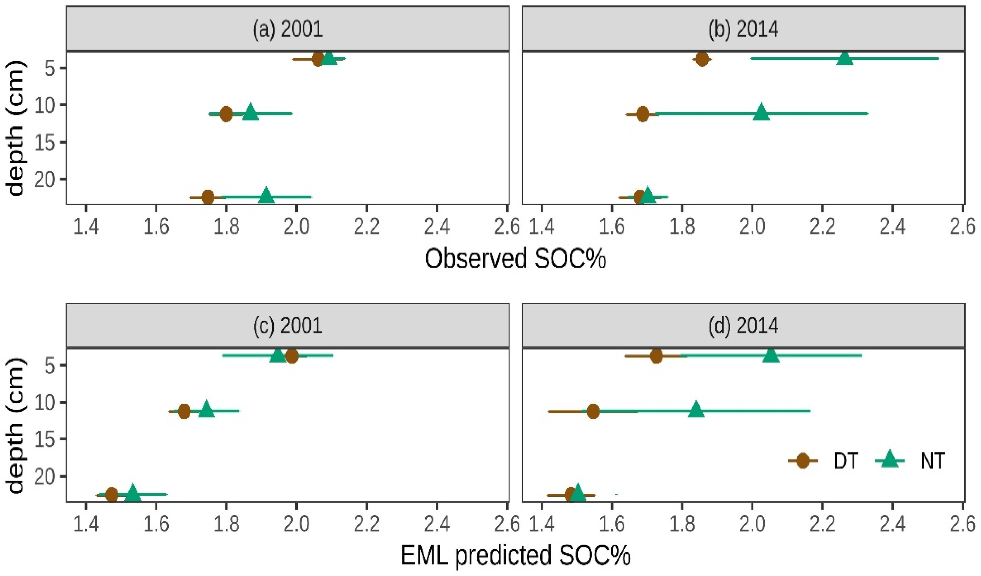
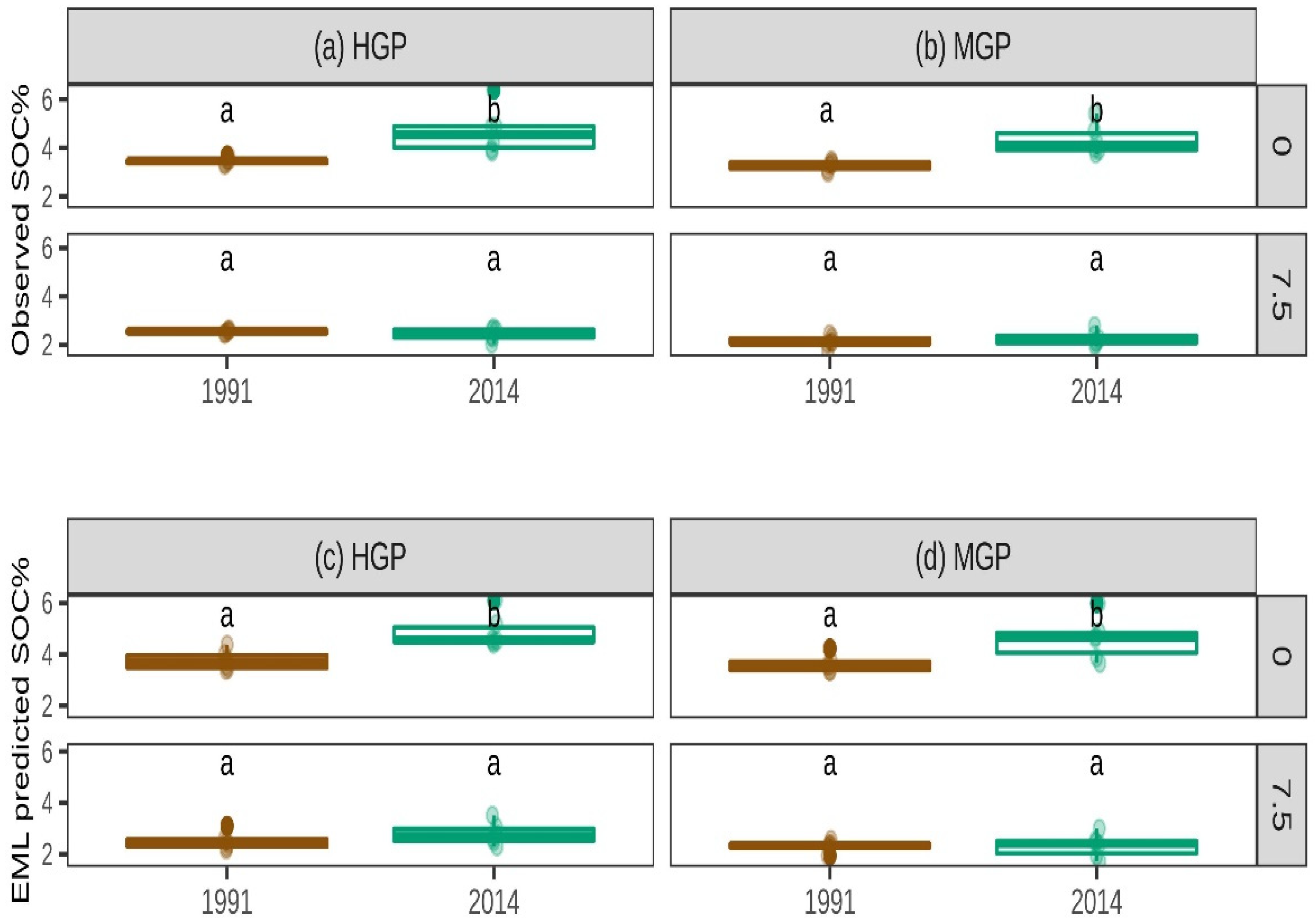
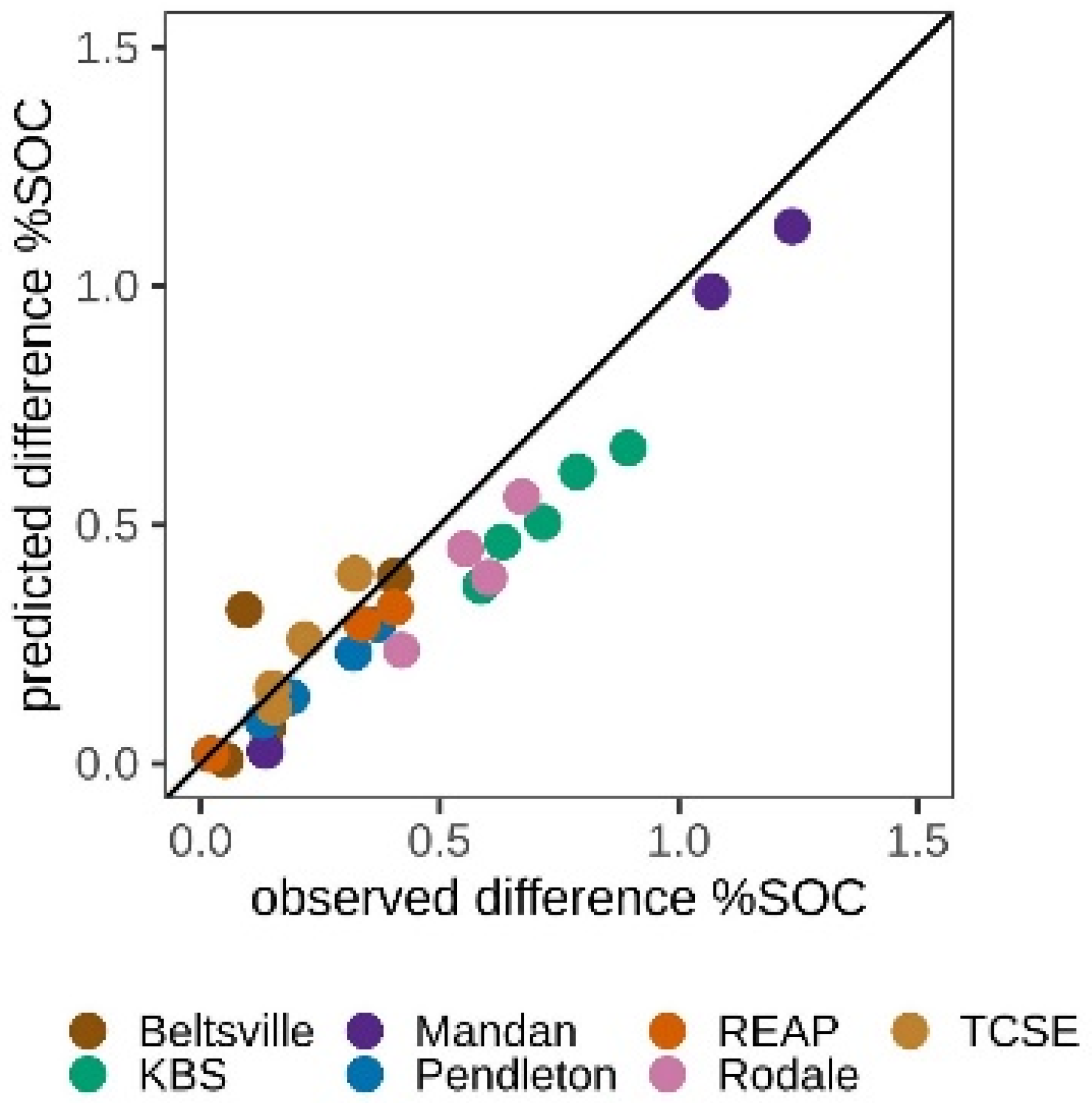
3.3. Detecting Changes in SOC% Across LTR Trials

Overall, the EML predicted SOC% were able to capture similar significant changes due to year, treatment and depth that were seen in a statistical analysis of the observed SOC% data for most of the LTR trials (

Table 4. Results from ANOVA models for each trial.

Trial	Model	Observed SOC% p-Value	m.ES a	EML SOC% p-Value	e.ES b
KBS	Treatment	2.53 × 10−11 ***	0.49	0.0005 ***	0.55
	n	28		28
Lincoln-REAP	Year	0.571	0	0.684	0.01
	Treatment	0.035 *	0.08	0.169	0.17
	Depth	0.009 **	0.41	0.002 ***	0.32
	Year × Treatment	0.290	0.05	0.287	0.05
	Year × Depth	0.674	0	0.941	0.03
	Treatment × Depth	0.774	0.02	0.790	0.02
	Year × Treatment × Depth	0.362	0.04	0.617	0.08
	n	72		72
Lincoln-TCSE	Year	0.563	0	0.252	0.01
	Treatment	0.000 ***	0.17	0.003 **	0.11
	Depth	1.84 × 10−11 ***	0.38	4.01 × 10−7 ***	0.24
	Year × Treatment	0.944	0	0.960	0
	Year × Depth	0.838	0	0.925	0
	Treatment × Depth	0.853	0	0.936	0
	Year × Treatment × Depth	0.925	0	0.916	0
	n	54		54
Rodale	Treatment	0.019 *	0.51	0.001 **	0.47
	n	32		32
Mandan	Year	4.94 × 10−5 ***	0.31	0.0001 ***	0.34
	Treatment	0.031 *	0.08	0.068 +	0.11
	Depth	2.50 × 10−15 ***	0.79	4.07 × 10−15 ***	0.79
	Year × Treatment	0.881	0.01	0.491	0
	Year × Depth	6.72 × 10−5 ***	0.20	0.003 **	0.33
	Treatment × Depth	0.929	0	0.652	0
	Year × Treatment × Depth	0.424	0	0.831	0.02
	n	48		48
Pendleton	Year	0.001 **	0.10	0.042 *	0.21
	Treatment	5.14 × 10−7 ***	0.41	8.38 × 10−6 ***	0.47
	Year × Treatment	0.147	0.02	0.962	0.15
	n	72		72
Beltsville	Year	0.165	0.08	0.377	0.05
	Treatment	0.004 **	0.31	0.635	0.06
	Year × Treatment	0.121	0.25	0.498	0.15
	n	56		56

N = total number of samples, m.ES ^a observed, e.ES ^b EML effective size calculated among treatments (units SOC%). ES values ~ 0.2 small effect, ~0.5 medium effect and ~0.8 large effect. Lincoln-TCSE, Lincoln-REAP, Mandan 3-way ANOVA. Beltsville, Pendleton, 2-way ANOVA, Rodale 1-way ANOVA and KBS repeated measures ANOVA. For KBS, sample years were used as repeated measurements across treatments. Bold indicates where EML data captured significant differences among years, treatment and depths also captured in the observed data. Underlined indicates observed and EML show differing significant results. The least significant difference (LSD) for ANOVA model using treatment for each trial is shown in Table S4. significance level p values were assigned as *** <0.001, ** <0.01, * <0.05, and + <0.10

). However, there were two cases (Lincoln REAP and Beltsville) where significant treatment effects were captured in the dry combustion data but not the EML predicted SOC% data suggesting that there is some trade-off of increased error associated with the rapid low-cost predictions.

At the Rodale LTR site, both observed and EML-predicted SOC% captured the same differences across the six management practices for the year 2015 (Table 4, Figure 3).

At the KBS trial, the EML predictions were able to detect a significant difference across treatments consistent with those detected in the observed SOC% data (Table 4, Figure S2). Among the treatments at the KBS trials, EML-predicted and observed SOC% trends over time were similar for five of the six treatments (Figure 4) with no significant differences in slopes likely due to the high year-to-year variability seen in a few of the treatments.

Significant differences with depths were detected in observed SOC% at the Lincoln-REAP trial (Table 4) as well as between two contrasting treatments (disk tilled with stubble removed and no-till with stubble retained, Figure 5). The treatment effects were most evident in the upper (10 cm) soil depths (Figure 5). However, EML-predicted SOC% across treatments, while following the same trend but at lower absolute values (Figure 5), was not able to capture the observed significant relationship across treatments (Table 4). Similarly, the observed SOC% from the Beltsville treatments showed significant differences among trials but the same trends could not be reproduced with EML-based estimates of SOC% (Figure S3, Table 4).

The Mandan LTR site showed significant changes over years and depths (Table 4) detected by observed and EML-predicted SOC%. Here, changes in SOC% within the upper 0–7.5 cm depth were detected in both observed and EML-predicted data between high and moderate grazing treatments over the 13 years (Table 4, Figure 6). The effects of the treatment on SOC% were not seen in the second depth increment (7.5–15 cm).

At the Lincoln-TCSE trial, observed and EML-predicted SOC% detected significant change across treatments and depths (Table 4). Differences among treatments at Lincoln-TCSE within years 1999 and 2011 (Figure S4) were detected, particularly between no-till and plow. Within years at the Pendleton trials, differences were detected in 2014 between no till (NTA) fertilizer treatments (Figure S5).

Given that the EML predictions were biased towards lower SOC% values (Table 2), we were interested in investigating whether or not the magnitude of the trial induced change in SOC% was also biased low. In Figure 7, the difference in SOC% between the highest SOC% treatment and the other treatments at each LTR trial, or over time in the case of Mandan, was calculated using the observed and EML predicted SOC% data. Across the 28 main comparisons at the seven sites, there was a small bias (0.07%) towards the EML predictions estimating a smaller difference than found in the observed data.

4. Discussion

4.1. How Well Can Spectroscopy Predict Soil Organic Carbon?

In this study we applied a national MIR spectral library to newly scanned samples in a different laboratory to test the ability of MIR spectroscopy to predict changes in SOC% over time for seven LTR sites. Across all LTR sites, we found that the spectroscopy-based predictions provided accurate estimates of SOC% with CCC = 0.92, RMSE = 0.24% and RPD = 3.40 (Figure 2, Table 2). While these overall performance metrics are quite good, there was a systematic underprediction using spectroscopy-based estimates of SOC% with the mean EML predictions being 0.23% lower than the mean observed SOC% (Table S3).

A more subtle test of the performance of the spectroscopy-based estimates was revealed by the goodness-of-fit at each LTR site individually where the underlying soil type was similar and alternative management strategies were driving much of the difference in SOC%. The average RMSE across all seven LTR sites was 0.18 ± 0.06% (95% CI) with an average RPD of 2.84 ± 0.57 (95% CI). The two trials where only one soil depth was collected (KBS and Rodale) had lower but still good performance with RPD values of 1.82 and 2.37, respectively (Table 2), likely due to a much narrower range in SOC% and lower sample size. Based on CCC, Pendleton and Rodale had the lowest performance suggesting slightly different reasons for lack of fit across the sites with some sites having higher accuracy at the cost of precision and others higher precision at the cost of accuracy.

Overall, these findings compare well with previously published estimates of spectroscopy-based model performance for SOC%. Soriano-Disla et al. [9] reported the median R² of 20 studies predicting SOC% was 0.93. The performance for prediction of SOC% using the KSSL MIR spectral library with advanced ML methods results in unbiased predictions with R² > 0.98 [11,15,16]. While the model performance for some of the individual LTR sites (Table 2) is on the lower end of the range in the recent literature, comparing the model performance presented in this work with these previous findings is not necessarily a fair comparison. This current work is a much more nuanced test of spectroscopy-based estimation of SOC% for three reasons: (1) each LTR site is dominated by one soil type so much of the variance in SOC% was due to management induced changes in SOC%; (2) no local samples were added to the calibration set; and (3) the predictions were made on spectra collected on a different instrument than the training library was developed on.

The addition of a small number of samples with analytical data that are representative of the target area to be predicted, often termed spiking, has been shown to greatly increase model performance [8,44]. For example, Seidel et al. [45] found that spiking the European LUCAS VNIR spectral library with as few as 15 samples tripled the RPD primarily due to the elimination of strong bias without the spiked local samples. Similarly, Lobsey et al. [46] found large improvements in performance after spiking a global VNIR spectral library with only 20 local samples. In this present study using a national MIR spectral library, we found that the use of memory-based learning applied to a national MIR spectral library resulted in performance levels without spiking that were as good as these two examples after spiking. It is possible that spiking would improve the local accuracy especially at the worst performing LTR sites in this study.

The need to account for differences in instruments and scanning conditions has been recognized for some time [47] and is recently gaining greater attention. Here, we have used a calibration transfer function developed by [17] to correct the Woodwell spectra to better match the KSSL spectral library. For a subset of 240 samples that were scanned at both Woodwell and the KSSL, we found that the additional uncertainty introduced by scanning on a secondary instrument and applying a calibration transfer function was an increase in RMSE of 0.03% and a reduction in R² of 0.02. For comparison, Dangal and Sanderman, [17] found that without calibration transfer the RMSE of a diverse set of soil samples increased from 0.71 to 1.84% but the calibration transfer function was able to bring the RMSE down to 1.26%.

We found a clear bias towards underprediction, mostly confined to samples with SOC% < 1.0, with the samples scanned at Woodwell compared to on the primary instrument at the KSSL. Table 3 indicated that there was negligible bias when the samples were scanned on the primary instrument but the bias was 0.25% when scanned at Woodwell. In our previous work [17], bias improved with calibration transfer but was not eliminated for most soil properties. This is an important finding and warrants further investigation into the causes of the bias, especially at low SOC values, and into ways of overcoming the bias. Other calibration transfer approaches such as spectral space transformation might overcome this issue [18].

The spectroscopy-based SOC% estimates (Figure 2) were quite good especially given that the observed SOC% data were generated in different laboratories than used in building the KSSL library. There is growing recognition that variability in the analytical data used in model building is at least as important to account for as variability in the spectra themselves [7,48]. The difference in the slopes of the observed versus predicted regression lines at each trial (Table 2) suggests that there may be a systematic bias between the local SOC% method and the SOC% measurements at the KSSL. Although, the fact that there was no bias when the samples were scanned at the KSSL suggests that some of this site-to-site bias may have been caused by the calibration transfer process. Despite SOC% determination by dry combustion being widely recognized as more accurate and reproducible than wet chemical methods (i.e., [49]) or estimation from loss-on-ignition [50], results from the Soil Science Society of America’s North American Proficiency Testing Program (NAPT) suggest non-negligible inter-laboratory differences in SOC% determined by dry combustion. For the 20 standard soil samples analyzed for SOC% in 2020 by about 15 different labs (https://www.naptprogram.org/content/laboratory-results, accessed on 20 March 2021), the mean of the median absolute deviation was 0.10% with a range from 0.21 to 0.30%. This reported inter-laboratory variance in SOC% is slightly lower but of similar magnitude to the reported mean absolute error (MAE) ranging from 0.15 to 0.39% across the seven LTR sites (Table 2). Future work with spectroscopy should include routine inclusion in proficiency testing programs to better understand the absolute performance of the method relative to dry combustion for quantifying SOC.

4.2. Can Spectroscopy Detect Changes in Soil Organic Carbon Due to Management?

Detecting statistically significant change in SOC% due to shifts in agricultural management over time is difficult due to a combination of the naturally spatial heterogeneous nature of SOC% distribution in the soil [51,52] and the small expected annual changes in SOC% relative to baseline levels [53,54]. Replicated and randomized field trials such as the seven LTR trials used in this study try to minimize the influence of spatial heterogeneity to enable even small but real management impacts to be more clearly observed [55,56]. In this study, we were interested in understanding if MIR spectroscopy-based estimates of SOC% would introduce enough additional uncertainty to make detecting real but small changes in SOC% impossible at the same sampling intensity.

The findings in this study indicate that the same conclusions would be drawn from these LTR trials regardless of the use of laboratory or spectroscopy-based estimates of SOC% in five of the seven trials at a significance level of 0.1 (Table 4). At the KBS main cropping system experiment, the linear slopes of change over time were similar using the two sources of SOC% data (Figure 4) and the relative ranking of SOC% levels across treatments were also the same (Figure S2). The same relative ranking and significant differences in SOC% levels regardless of using lab-based or spectroscopy-based data were also seen across Rodale treatments (Figure 3). At the Lincoln-TCSE trial, there was a significant tillage effect (Table 4) with the no-till treatments having higher SOC% than either disk or mold-board tillage regardless of SOC% method (Figure S4). The trends at the Lincoln-TCSE trial were consistent with results from a different 2011 soil sampling campaign which found that plowed soils had significantly lower SOC% than the no-till treatment in the upper 15 cm [57].

At the one grazed grassland site, Mandan, the same significant differences over time and across treatments were found when using the observed SOC% and spectroscopy-based estimates of SOC% (Figure 6). These estimates aligned with previous investigations at Mandan, where [29] found that near-surface SOC% (0–7.6 cm) increased between 1991 and 2014 from 3.3 to 4.4% under moderate grazing intensity, and from 3.4 to 4.8% under heavy grazing intensity. Similarly, soil profile assessments (0–60 cm) between 1959 and 2003 found soil C accrual rates of 0.39 and 0.41 Mg C ha⁻¹ year⁻¹ for moderate and heavy grazing, respectively [30].

There were two cases where the spectroscopy estimates did not capture the same changes in SOC%, at a significance level of p < 0.10, due to management as was observed in the lab-based SOC% dataset. At both the Lincoln-REAP trial and the Beltsville trial, the trends were in the same direction but the introduction of additional variance coupled with small effect sizes (Table 4) precluded statistical significance (Figure 5 and Figure S3). In both of these cases, it is possible but unclear if an increased sampling effort would have enabled the detection of significant treatment effects. At Beltsville, the overall low SOC% values (mean = 0.89%, Q25 = 0.24%) could be another contributing factor to the discrepancy between the lab and spectroscopy-based results. With low SOC values, even small additional uncertainty can swamp the ability to detect statistical change.

In the last section, we raised the concern that the EML predictions were consistently biased towards lower SOC% values; however, the trial ANOVA tests suggested that change in SOC% can still be detected. More encouragingly, Figure 7 indicated that the magnitude of difference between treatments was mostly preserved with a bias in estimating SOC% change of only 0.07% compared with a bias in estimating SOC% of 0.23% (Table 2).

5. Conclusions

Spectroscopy has an important role to play in carbon monitoring because it can substantially reduce the cost of SOC measurement. Nearly all previous work has tested the performance of soil spectroscopy against spatially distinct soil samples. Here, we tested whether MIR spectroscopy can measure subtle management-induced changes in SOC% in the same soil over time. Across seven LTR sites, the spectroscopy-based results were compared very favorably with traditional dry combustion data, albeit with an average bias of 0.23%, and in most cases, the same statistical trends were found using either the observed or the predicted SOC% data. Improvements in calibration transfer are necessary to eliminate the consistent bias at low SOC% values found in this study. Our findings suggest that large existing MIR spectral libraries can be operationalized in other laboratories for successful carbon monitoring. The reduced cost and increased throughput afforded by soil spectroscopy can allow for greater sample numbers likely overcoming any additional variance introduced by the indirect estimation of SOC.

References

1. Bossio, D.A.; Cook-Patton, S.C.; Ellis, P.W.; Fargione, J.; Sanderman, J.; Smith, P.; Wood, S.; Zomer, R.J.; von Unger, M.; Emmer, I.M.; et al. The Role of Soil Carbon in Natural Climate Solutions. Nat. Sustain. 2020, 3, 391–398. [Google Scholar] [CrossRef]
2. CFI 2018-Carbon Credits (Carbon Farming Initiative—Measurement of Soil Carbon Sequestration in Agricultural Systems) Methodology Determination 2018. Available online: www.legislation.gov.au/Details/F2018L00089 (accessed on 20 March 2021).
3. Smith, P.; Soussana, J.F.; Angers, D.; Schipper, L.; Chenu, C.; Rasse, D.P.; Batjes, N.H.; van Egmond, F.; McNeill, S.; Kuhnert, M.; et al. How to Measure, Report and Verify Soil Carbon Change to Realize the Potential of Soil Carbon Sequestration for Atmospheric Greenhouse Gas Removal. Glob. Chang. Biol. 2020, 26, 219–241. [Google Scholar] [CrossRef] [Green Version]
4. Bellon-Maurel, V.; McBratney, A. Near-Infrared (NIR) and Mid-Infrared (MIR) Spectroscopic Techniques for Assessing the Amount of Carbon Stock in Soils-Critical Review and Research Perspectives. Soil Biol. Biochem. 2011, 43, 1398–1410. [Google Scholar] [CrossRef]
5. Nocita, M.; Stevens, A.; van Wesemael, B.; Aitkenhead, M.; Bachmann, M.; Barthès, B.; Dor, E.B.; Brown, D.J.; Clairotte, M.; Csorba, A.; et al. Soil Spectroscopy: An Alternative to Wet Chemistry for Soil Monitoring. Adv. Agron. 2015, 132, 139–159. [Google Scholar] [CrossRef]
6. Gholizadeh, A.; Luboš, B.; Saberioon, M.; Vašát, R. Visible, near-Infrared, and Mid-Infrared Spectroscopy Applications for Soil Assessment with Emphasis on Soil Organic Matter Content and Quality: State-of-the-Art and Key Issues. Appl. Spectrosc. 2013, 67, 1349–1362. [Google Scholar] [CrossRef] [PubMed]
7. Viscarra Rossel, R.A.; Walvoort, D.J.J.; McBratney, A.B.; Janik, L.J.; Skjemstad, J.O. Visible, near Infrared, Mid Infrared or Combined Diffuse Reflectance Spectroscopy for Simultaneous Assessment of Various Soil Properties. Geoderma 2006, 131, 59–75. [Google Scholar] [CrossRef]
8. Shepherd, K.D.; Walsh, M.G. Development of Reflectance Spectral Libraries for Characterization of Soil Properties. Soil Sci. Soc. Am. J. 2002, 66, 988–998. [Google Scholar] [CrossRef]
9. Soriano-Disla, J.M.; Janik, L.J.; Viscarra Rossel, R.A.; MacDonald, L.M.; McLaughlin, M.J. The Performance of Visible, near-, and Mid-Infrared Reflectance Spectroscopy for Prediction of Soil Physical, Chemical, and Biological Properties. Appl. Spectrosc. Rev. 2014, 49, 139–186. [Google Scholar] [CrossRef]
10. Clairotte, M.; Grinand, C.; Kouakoua, E.; Thébault, A.; Saby, N.P.A.; Bernoux, M.; Barthès, B.G. National Calibration of Soil Organic Carbon Concentration Using Diffuse Infrared Reflectance Spectroscopy. Geoderma 2016, 276, 41–52. [Google Scholar] [CrossRef]
11. Ng, W.; Minasny, B.; Montazerolghaem, M.; Padarian, J.; Ferguson, R.; Bailey, S.; McBratney, A.B. Convolutional Neural Network for Simultaneous Prediction of Several Soil Properties Using Visible/near-Infrared, Mid-Infrared, and Their Combined Spectra. Geoderma 2019, 352, 251–267. [Google Scholar] [CrossRef]
12. Reeves, J.B. Near- versus Mid-Infrared Diffuse Reflectance Spectroscopy for Soil Analysis Emphasizing Carbon and Laboratory versus on-Site Analysis: Where Are We and What Needs to Be Done? Geoderma 2010, 158, 3–14. [Google Scholar] [CrossRef]
13. Griffiths, P.R.; de Haseth, J.A. Fourier Transform Infrared Spectrometry, 2nd ed.; John Wiley & Sons: Hoboken, NJ, USA, 2006. [Google Scholar]
14. Baldock, J.A.; Hawke, B.; Sanderman, J.; MacDonald, L.M. Predicting Contents of Carbon and Its Component Fractions in Australian Soils from Diffuse Reflectance Mid-Infrared Spectra. Soil Res. 2013, 51, 577–595. [Google Scholar] [CrossRef] [Green Version]
15. Dangal, S.; Sanderman, J.; Wills, S.; Ramirez-Lopez, L. Accurate and Precise Prediction of Soil Properties from a Large Mid-Infrared Spectral Library. Soil Syst. 2019, 3, 11. [Google Scholar] [CrossRef] [Green Version]
16. Wijewardane, N.K.; Ge, Y.; Wills, S.; Libohova, Z. Predicting Physical and Chemical Properties of US Soils with a Mid-Infrared Reflectance Spectral Library. Soil Sci. Soc. Am. J. 2018, 82, 722–732. [Google Scholar] [CrossRef] [Green Version]
17. Dangal, S.R.S.; Sanderman, J. Is Standardization Necessary for Sharing of a Large Mid-Infrared Soil Spectral Library? Sensors 2020, 20, 6729. [Google Scholar] [CrossRef] [PubMed]
18. Pittaki-Chrysodonta, Z.; Hartemink, A.E.; Sanderman, J.; Ge, Y.; Huang, J. Evaluating Three Calibration Transfer Methods for Predictions of Soil Properties Using Mid-infrared Spectroscopy. Soil Sci. Soc. Am. J. 2021, 85, 501–519. [Google Scholar] [CrossRef]
19. Feudale, R.N.; Woody, N.A.; Tan, H.; Myles, A.J.; Brown, S.D.; Ferré, J. Transfer of Multivariate Calibration Models: A Review. Chemom. Intell. Lab. Syst. 2002, 64, 181–192. [Google Scholar] [CrossRef]
20. Workman, J.J. A Review of Calibration Transfer Practices and Instrument Differences in Spectroscopy. Appl. Spectrosc. 2018, 72, 340–365. [Google Scholar] [CrossRef] [PubMed]
21. Seybold, C.A.; Ferguson, R.; Wysocki, D.; Bailey, S.; Anderson, J.; Nester, B.; Schoeneberger, P.; Wills, S.; Libohova, Z.; Hoover, D.; et al. Application of Mid-Infrared Spectroscopy in Soil Survey. Soil Sci. Soc. Am. J. 2019, 83, 1746–1749. [Google Scholar] [CrossRef]
22. CAR 2020 Climate Action Reserve 2001–2020. Available online: www.climateactionreserve.org/how/projects/ (accessed on 20 March 2021).
23. Sanderman, J.; Savage, K.; Dangal, S.R.S. Mid-Infrared Spectroscopy for Prediction of Soil Health Indicators in the United States. Soil Sci. Soc. Am. J. 2020, 84, 251–261. [Google Scholar] [CrossRef] [Green Version]
24. Robertson, G.P.; Hamilton, S.K. Long-Term Ecological Research at the Kellogg Biological Station LTER Site: Conceptual and Experimental Framework. In The Ecology of Agricultural Landscapes: Long-Term Research on the Path to Sustainability; Hamilton, S.K., Doll, J.E., Robertson, G.P., Eds.; Oxford University Press: New York, NY, USA, 2015; pp. 1–32. [Google Scholar]
25. Jin, V.L.; Schmer, M.R.; Wienhold, B.J.; Stewart, C.E.; Varvel, G.E.; Sindelar, A.J.; Follett, R.F.; Mitchell, R.B.; Vogel, K.P. Twelve Years of Stover Removal Increases Soil Erosion Potential without Impacting Yield. Soil Sci. Soc. Am. J. 2015, 79, 1169–1178. [Google Scholar] [CrossRef]
26. Follett, R.F.; Vogel, K.P.; Varvel, G.E.; Mitchell, R.B.; Kimble, J. Soil Carbon Sequestration by Switchgrass and No-Till Maize Grown for Bioenergy. Bioenergy Res. 2012, 5, 866–875. [Google Scholar] [CrossRef] [Green Version]
27. Sindelar, A.J.; Schmer, M.R.; Jin, V.L.; Wienhold, B.J.; Varvel, G.E. Long-Term Corn and Soybean Response to Crop Rotation and Tillage. Agron. J. 2015, 107, 2241–2252. [Google Scholar] [CrossRef] [Green Version]
28. Hepperly, P.; Seidel, R.; Pimentel, D.; Hanson, J.; Douds, D. Organic farming enhances soil carbon and its benefits. In Soil Carbon Management; Kimble, J.M., Rice, C.W., Reed, D., Mooney, S., Follett, R.F., Lal, R., Eds.; CRC Press: Boca Raton, FL, USA, 2007; pp. 130–150. [Google Scholar]
29. Sanderson, M.A.; Johnson, H.; Liebig, M.A.; Hendrickson, J.R.; Duke, S.E. Kentucky. Bluegrass Invasion Alters Soil Carbon and Vegetation Structure on Northern Mixed-Grass Prairie of the United States. Invasive Plant Sci. Manag. 2017, 10, 9–16. [Google Scholar] [CrossRef]
30. Liebig, M.A.; Gross, J.R.; Kronberg, S.L.; Phillips, R.L. Grazing Management Contributions to Net Global Warming Potential: A Long-Term Evaluation in the Northern Great Plains. J. Environ. Qual. 2010, 39, 799–809. [Google Scholar] [CrossRef] [PubMed]
31. Gollany, H.T.; DelGrosso, S.J.; Dell, C.J.; Adler, P.R.; Polumsky, R.W. Assessing the Effectiveness of Agricultural Conservation Practices in Maintaining Soil Organic Carbon under Contrasting Agroecosystems and Changing Climate. Soil Sci. Soc. Am. J. 2021, 1–18. [Google Scholar] [CrossRef]
32. Cavigelli, M.A.; Teasdale, J.R.; Conklin, A.E. Long-Term Agronomic Performance of Organic and Conventional Field Crops in the Mid-Atlantic Region. Agron. J. 2008, 100, 785–794. [Google Scholar] [CrossRef] [Green Version]
33. White, K.E.; Cavigelli, M.A.; Conklin, A.E.; Rasmann, C. Economic Performance of Long-Term Organic and Conventional Crop Rotations in the Mid-Atlantic. Agron. J. 2019, 111, 1358–1370. [Google Scholar] [CrossRef]
34. Roudier, P. Clhs: A R Package for Conditioned Latin Hypercube Sampling. 2011. Available online: https://cran.r-project.org/web/packages/clhs/clhs.pdf (accessed on 20 March 2021).
35. R. Core Team (2020). R: A Language and Environment for Statistical Computing; R Foundation for Statistical Computing: Vienna Austria, 2020; Available online: https://www.r-project.org/ (accessed on 20 March 2021).
36. Ramirez-Lopez, L.; Behrens, T.; Schmidt, K.; Stevens, A.; Demattê, J.A.M.; Scholten, T. The Spectrum-Based Learner: A New Local Approach for Modeling Soil Vis-NIR Spectra of Complex Datasets. Geoderma 2013, 195–196. [Google Scholar] [CrossRef]
37. Ramirez-Lopez, L.; Stevens, A. Resemble: Regression and Similarity Evaluation for Memory-Based Learning in Spectral Chemometrics, R Package Version. 2019. Available online: https://cran.r-project.org/web/packages/resemble/resemble.pdf(accessed on 20 March 2021).
38. Microsoft Corporation; Weston, S. DoSNOW: Foreach Parallel Adaptor for the “Snow”. Available online: https://cran.r-project.org/web/packages/doSNOW/doSNOW.pdf (accessed on 20 March 2021).
39. Lin, L.I.-K. A Concordance Correlation Coefficient to Evaluate Reproducibility. Biometrics 1989, 45, 255–268. [Google Scholar] [CrossRef]
40. De Mendiburu, F.; Yaseen, M. Statistical Procedures for Agricultural Research; John Wiley & Sons: Hoboken, NJ, USA, 1984. [Google Scholar]
41. Ben-Shachar, M.; Lüdecke, D.; Makowski, D. Effectsize: Estimation of Effect Size Indices and Standardized Parameters. J. Open Source Softw. 2020, 5, 1–7. [Google Scholar] [CrossRef]
42. Wickham, H. Ggplot2: Elegant Graphics for Data Analysis; Springer: New York, NY, USA, 2016; ISBN 978-3-319-24277-4. [Google Scholar]
43. Ahlmann-Eltze, C. Ggsignif: Significance Brackets for “Ggplot2”. R Package Version 0.6.0. 2019. Available online: https://cran.r-project.org/web/packages/ggsignif/ggsignif.pdf (accessed on 20 March 2021).
44. Brown, D.J. Using a Global VNIR Soil-Spectral Library for Local Soil Characterization and Landscape Modeling in a 2nd-Order Uganda Watershed. Geoderma 2007, 140, 444–453. [Google Scholar] [CrossRef]
45. Seidel, M.; Hutengs, C.; Ludwig, B.; Thiele-Bruhn, S.; Vohland, M. Strategies for the Efficient Estimation of Soil Organic Carbon at the Field Scale with Vis-NIR Spectroscopy: Spectral Libraries and Spiking vs. Local Calibrations. Geoderma 2019, 354, 113856. [Google Scholar] [CrossRef]
46. Lobsey, C.R.; Viscarra Rossel, R.A.; Roudier, P.; Hedley, C.B. Rs-Local Data-Mines Information from Spectral Libraries to Improve Local Calibrations. Eur. J. Soil Sci. 2017, 68, 840–852. [Google Scholar] [CrossRef] [Green Version]
47. Ge, Y.; Morgan, C.L.S.; Grunwald, S.; Brown, D.J.; Sarkhot, D.V. Comparison of Soil Reflectance Spectra and Calibration Models Obtained Using Multiple Spectrometers. Geoderma 2011, 161, 202–211. [Google Scholar] [CrossRef]
48. Viscarra Rossel, R.A.; Jeon, Y.S.; Odeh, I.O.A.; McBratney, A.B. Using a Legacy Soil Sample to Develop a Mid-IR Spectral Library. Soil Res. 2008, 46, 1–16. [Google Scholar] [CrossRef]
49. Walkley, A.; Black, I.A. An Examination of the Degtjareff Method for Determining Soil Organic Matter, and a Proposed Modification of the Chromic Acid Titration Method. Soil Sci. 1934, 37, 29–38. [Google Scholar] [CrossRef]
50. Pribyl, D.W. A Critical Review of the Conventional SOC to SOM Conversion Factor. Geoderma 2010, 156, 75–83. [Google Scholar] [CrossRef]
51. Cambardella, C.A.; Moorman, T.B.; Novak, J.M.; Parkin, T.B.; Karlen, D.L.; Turco, R.F.; Konopka, A.E. Field-Scale Variability of Soil Properties in Central Iowa Soils. Soil Sci. Soc. Am. J. 1994, 58, 1501–1511. [Google Scholar] [CrossRef]
52. Zhang, Y.; Hartemink, A.E. Quantifying Short-Range Variation of Soil Texture and Total Carbon of a 330-Ha Farm. Catena 2021, 201, 105200. [Google Scholar] [CrossRef]
53. Post, W.M.; Kwon, K.C. Soil Carbon Sequestration and Land-Use Change: Processes and Potential. Glob. Chang. Biol. 2000, 6, 317–327. [Google Scholar] [CrossRef] [Green Version]
54. Sanderman, J.; Baldock, J.A. Accounting for Soil Carbon Sequestration in National Inventories: A Soil Scientist’s Perspective. Environ. Res. Lett. 2010, 5, 1–7. [Google Scholar] [CrossRef]
55. Atkinson, A.C.; Bailey, R.A. One Hundred Years of the Design of Experiments on and off the Pages of Biometrika. Biometrika 2001, 88, 53–97. [Google Scholar] [CrossRef]
56. Van Es, H.M.; Gomes, C.P.; Sellmann, M.; van Es, C.L. Spatially-Balanced Complete Block Designs for Field Experiments. Geoderma 2007, 140, 346–352. [Google Scholar] [CrossRef]
57. Jin, V.L.; Wienhold, B.J.; Mikha, M.M.; Schmer, M.R. Cropping System Partially Offsets Tillage-Related Degradation of Soil Organic Carbon and Aggregate Properties in a 30-Yr Rainfed Agroecosystem. Soil Tillage Res. 2021, 209, 104968. [Google Scholar] [CrossRef]
Figure 1. Schematic diagram of workflow for spectra processing and ensemble machine learning (EML) model predictions.
Remotesensing 13 02265 g001
Figure 2. Soil OC% observed versus mean EML predicted SOC% using spectra collected at Woodwell for (a) all trials combined, (b) Beltsville, (c) KBS, (d) Mandan, (e) Pendleton, (f) Lincoln-REAP, (g) Rodale, and (h) Lincoln-TCSE. The LTR data are all observations across years, treatments, and depths (Table 1). Symbols are color coded by observation sample depth. Results of linear model fits (red lines) are found in Table 2. All slopes are significantly different from 1, except h) TCSE (p = 0.79). Vertical lines are 95% confidence intervals for EML predictions. Confidence intervals are tight at low SOC% and not visible across most plotting symbols.
Remotesensing 13 02265 g002
Figure 3. Box plots of observed (a) and EML predicted (b) SOC% for the 2015 Rodale trials. Test across similar management but with till vs no-till. t-test comparison, No significant difference between the same letters. Significance level <0.05. Sample size per treatment, CNVnt, CNVt n = 8 each, LEGnt, LEGt, MNRnt, MNRt n = 4 each (total 32).
Remotesensing 13 02265 g003
Figure 4. KBS trial treatment by sample year. (a) T1, (b) T2, (c) T3, (d) T4, (e) T6, (f) T8. See Table 1 for treatment description. No significant differences in slopes were detected.
Remotesensing 13 02265 g004
Figure 5. Lincoln-REAP trials mean and SE (n = 3) across depth (0–7.5, 7.5–15 and 15–30 cm) and years for observed (a,b) and EML-predicted (c,d) SOC%. Treatments DT— disk till with stover removal, NT—no-till with stover retention.
Remotesensing 13 02265 g005
Figure 6. Boxplot of observed and EML-predicted %SOC for the Mandan trials across years and depths (0–7.5 cm and 7.5–15 cm, n=6 per depth). (a,b) are observed SOC% for high and moderate grazed management. (c,d) are EML-predicted SOC% for high and moderate grazed management practices. No significant difference between the same letters. Significance level < 0.05.
Remotesensing 13 02265 g006
Figure 7. Observed versus EML predicted difference in SOC% between best management treatment and other treatments at each of the seven trials. At Mandan, the difference is between time points, not treatments.
Remotesensing 13 02265 g007