Article

Regional Mapping of Groundwater Potential in Ar Rub Al Khali, Arabian Peninsula Using the Classification and Regression Trees Model

1
GIS and Mapping Laboratory, Civil Engineering Department, College of Engineering, American University of Sharjah, Sharjah P.O. Box 26666, United Arab Emirates
2
Civil and Environmental Engineering Department, United Arab Emirates University, Al-Ain P.O. Box 15551, United Arab Emirates
3
National Water and Energy Center, United Arab Emirates University, Al Ain, Abu Dhabi P.O. Box 15551, United Arab Emirates
*
Author to whom correspondence should be addressed.
Remote Sens. 2021, 13(12), 2300; https://0-doi-org.brum.beds.ac.uk/10.3390/rs13122300
Submission received: 24 April 2021 / Revised: 4 June 2021 / Accepted: 7 June 2021 / Published: 11 June 2021
(This article belongs to the Section Remote Sensing in Geology, Geomorphology and Hydrology)

Abstract

:
Mapping of groundwater potential in remote arid and semi-arid regions underneath sand sheets over a very regional scale is a challenge and requires an accurate classifier. The Classification and Regression Trees (CART) model is a robust machine learning classifier used in groundwater potential mapping over a very regional scale. Ten essential groundwater conditioning factors (GWCFs) were constructed using remote sensing data. The spatial relationship between these conditioning factors and the observed groundwater wells locations was optimized and identified by using the chi-square method. A total of 185 groundwater well locations were randomly divided into 129 (70%) for training the model and 56 (30%) for validation. The model was applied for groundwater potential mapping by using optimal parameters values for additive trees were 186, the value for the learning rate was 0.1, and the maximum size of the tree was five. The validation result demonstrated that the area under the curve (AUC) of the CART was 0.920, which represents a predictive accuracy of 92%. The resulting map demonstrated that the depressions of Mondafan, Khujaymah and Wajid Mutaridah depression and the southern gulf salt basin (SGSB) near Saudi Arabia, Oman and the United Arab Emirates (UAE) borders reserve fresh fossil groundwater as indicated from the observed lakes and recovered paleolakes. The proposed model and the new maps are effective at enhancing the mapping of groundwater potential over a very regional scale obtained using machine learning algorithms, which are used rarely in the literature and can be applied to the Sahara and the Kalahari Desert.

Graphical Abstract

1. Introduction

Groundwater is an important source in land development and human activities such as agriculture and industry. Groundwater is one of the most important resources worldwide, especially in arid and semi-arid regions [1,2,3,4,5,6,7,8]. In arid and semi-arid regions, there has been excessive consumption of groundwater and scarce rainfall due to climate change and population growth [1,2]. These have led to sharp depletions in the groundwater table and the quality. These problems represent the challenge of developing such regions and are clearly demonstrated in the Arabian Peninsula countries, particularly Saudi Arabia and the United Arab Emirates [1]. About 50% of these countries lay within the largest sand sea in the world, which is known as ARAK. It is the largest promising groundwater aquifer in the world and sits on top of a vast amount of fossil water reserves [1,2,3]. The hydrological setting of the ARAK is explored only from oil wells and geophysical reports over a local scale due to its harsh weather, remote location and lack of rock outcrops [2,3]. However, the remote sensing data have proven to be excellent tools for mapping surface and near-surface paleochannels, drainage basins, zones of groundwater potential and for retrieval of soil moisture over a regional scale [4,5,6,7,8]. Groundwater potential zones can be defined as the areas that reserve a considerable amount of groundwater or fossil water [1,2,3]. Locally, a limited number of studies have been applied to map near-surface fluvial channels delineated paleolake beds and the fluvial channels in the Jafurah sand field and the ARAK from the Shuttle Imaging Radar (SIR-C) imageries using manual screen digitizing [9,10]. However, this traditional technique introduces bias and errors [11]. Sultan et al. (2008) [12] automatically mapped the major paleochannels using the Shuttle Radar Topographic Mission (SRTM) DEM. They investigated the evolution of the ARAK aquifer using geochemical information collected from groundwater wells. Several studies have been achieved to model groundwater potential in a GIS environment integrated with Frequency Ratio (FR), Logistic Regression (LR), Weights of Evidence (WofE), Information Value (IV) and Shannon’s Entropy (SE) [9,10,11,12,13,14]. Further studies have been applied to susceptibility map geohazard and groundwater using machine learning such as Boosted Regression Tree (BRT), Classification and Regression Tree (CART), and Random Forest (RF) [15,16,17,18,19,20,21,22,23,24,25,26,27,28,29,30]. The CART has been applied to predict pulmonary tuberculosis in hospitalized patients [31]. The results of these studies show that the CART has a high predictive ability and had better performance than multivariate models [23,27]. The CART saves some computer time and is superior to categorical predictors, so it can be used for mapping groundwater potential over a very regional scale [27]. Therefore, this study aims to explore the effectiveness of the machine learning of mapping over a very regional scale, along with the applicability of the CART for groundwater potential. The CART, which is used widely in the literature provides the basis for important algorithms such as bagged decision, random forest and boosted decision trees [32]. This study is a new application of the CART for mapping groundwater potential over a very regional scale and represents an advanced step to develop predictable regional maps of groundwater potential created using a single machine learning model in an arid region. This study fills the gap in the hydrological information and permits a better understanding of the hydrological setting of the ARAK. Understanding the hydrological setting is important for better hydrological management of the ARAK and exploration of additional sites of groundwater.

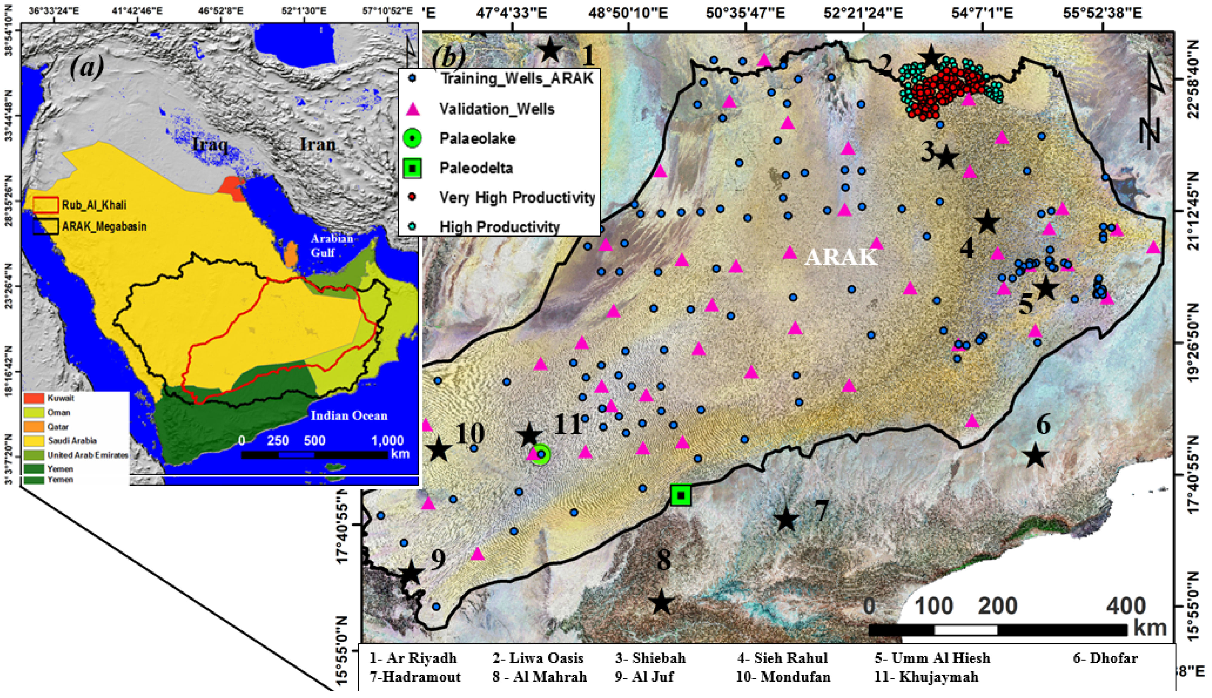
2. Description of the Study Area

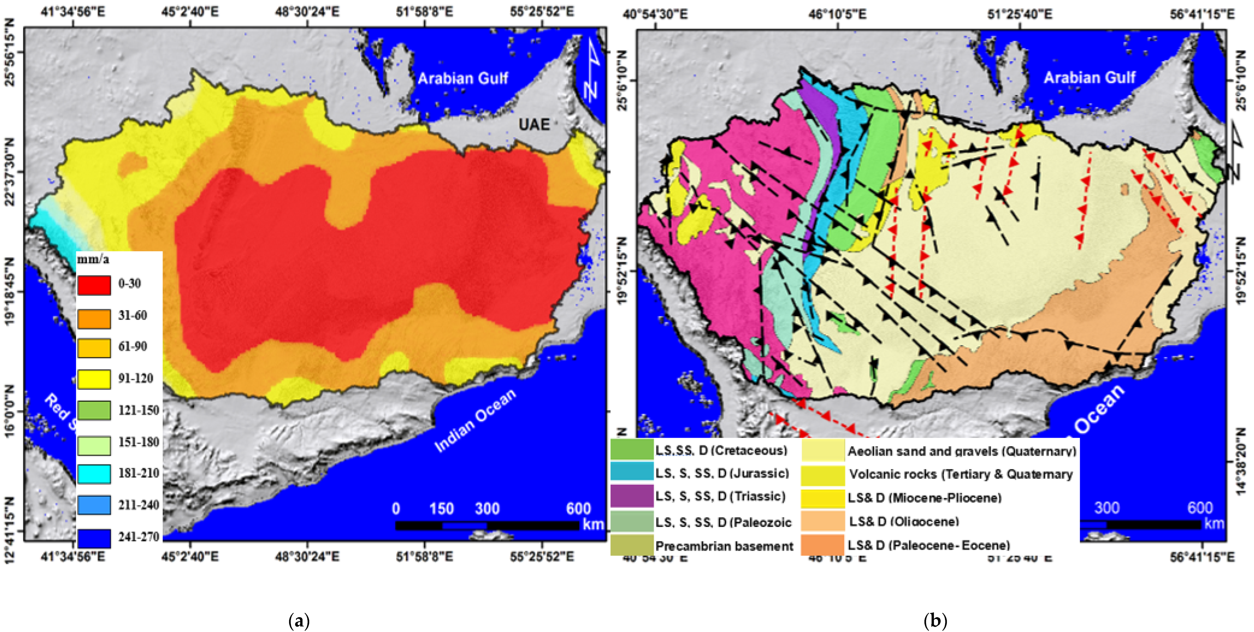
2.1. Geography and Topographic

The study area, which includes Ar Rub Al Khali (the Empty Quarter) mega-basin and its aquifer underneath the sand sheets, stretches from longitude 40°54′15″E to 56°41′20″E and latitude from 14°15′20″N to 25°11′23″N and covers an area of about 557,467 km2 (Figure 1). The ARAK region includes the ARAK aquifer underneath the sand sheets and its adjoining mountainous areas (sources of recharge). The ARAK region occupies an area of about 1,173,973 km2 and its aquifer is covered by the largest sand dune hills deposited during the pluvial and interpluvial periods of the Tertiary and Quaternary [33,34,35,36]. It is one of the largest aquifers in the world underlying sand sea and extending among the Kingdom of Saudi Arabia, the United Arab Emirates, the Sultanate of Oman and the Republic of Yemen (Figure 1).
The ARAK aquifer is located within arid and semiarid regions, inaccessible terrain due to its harsh climatic conditions. It is characterized by a hot dry climate, and temperature ranges from 41 °C to 55 °C during summer and from 15 °C to 27 °C during winter. The monthly rainfall during summer is low and ranges from 0 to 14 mm and could reach above 700 mm during October over the adjoining mountainous areas such as Asser, Hejaz and Juf in the west and southwest (Figure 2a). Other regions such as the Riyad hills (northeast) and Hadramout (south) and Oman (east) mountains experience waves of precipitation varying from 90 to 220 mm that is a function of groundwater recharge, which varies from 0% to 4% [37].
Similar to the Eastern Sahara, the aquifers have received a considerable amount of water during wet periods that prevailed during the Late Pleistocene and Late Quaternary, as indicated by lacustrine, evaporite (sabkha) and playa carbonate deposits and paleochannels that are very closely associated with terminal desiccation of paleolake events [5,28,38,39,40,41,42,43,44,45,46,47]. Topographically, the ARAK aquifer area is surrounded by mountainous areas with elevation ranges from 50 m near the Saudi Arabia and UAE borders to 3500 m in the Aseer mountains (Figure 2b). The ARAK aquifer area is dotted by several paleolakes with depth ranges from 2 to 10 m, produced by cataclysmic rainfall and with no links with rivers, and their bed sediment presents no evidence of regular filling [48,49] (green points in Figure 1b). These features were described as lacustrine calcareous and/or clay and silt. They were observed to be governed by the shallow water table, which endorses evaporation and resulting gypsum, calcite, and anhydrite [49].

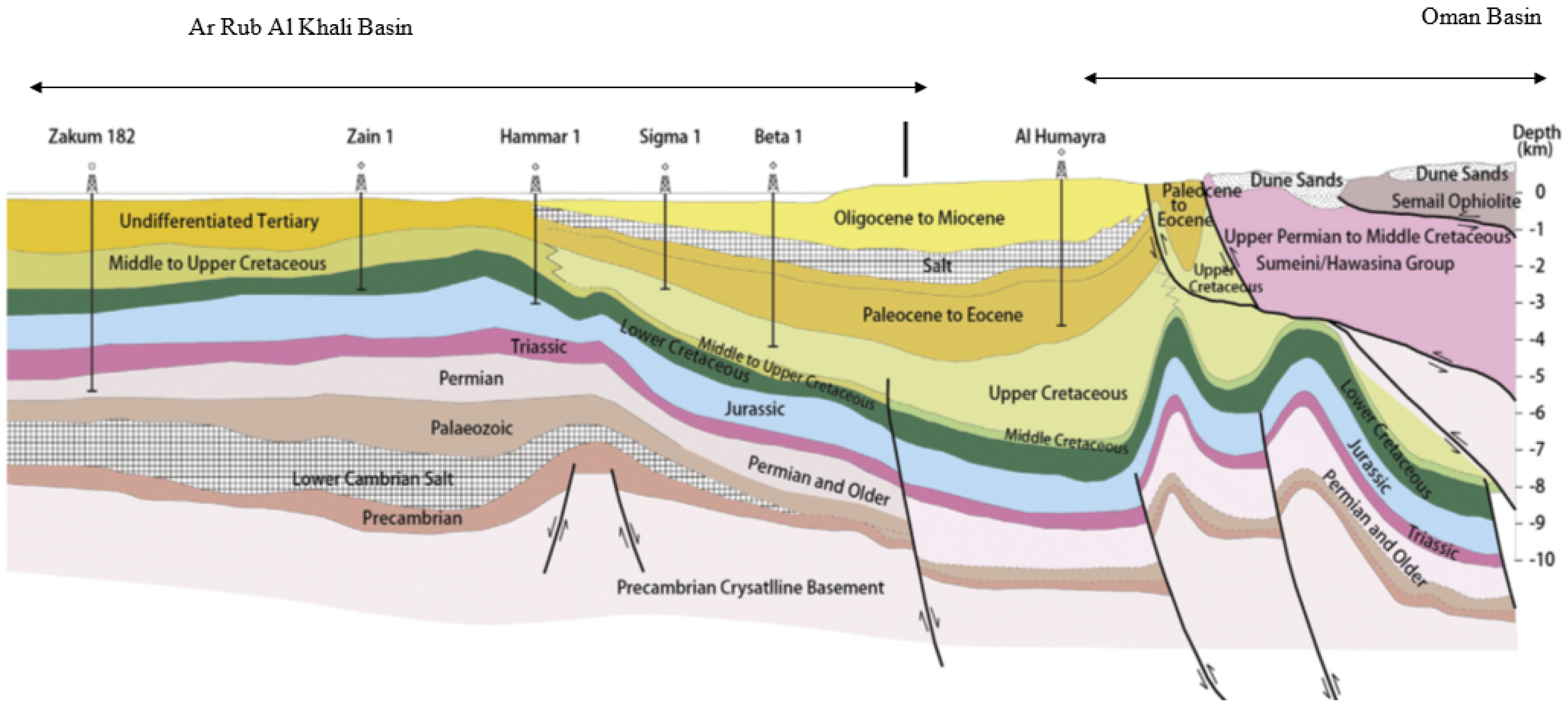
2.2. Geology and Hydrology

The ARAK aquifer area consists of a thick stratigraphic succession of sedimentary rocks belonging to Cambrian to recent and overlying the Precambrian basement of rugged rocks that are cropped out in the Red Sea [50]. Historically, the Arabian Peninsula experienced several tectonic events, creating several regional faults, folds, grabens and hydrological basins (Figure 2b) [3]. These structures are distributed in Wajid, Armad near the state of Qatar, at the foot of the Oman mountains in the east and in Al Juf and Asser mountains in the west and southwest. Other basins and grabens are found near the UAE and Saudi Arabia border [34,40,50,51]. Their directions were found to be in the NW–SE, N–S, NNE–SSW and NE–SW directions (Figure 2b).
These geological structures have led to dipping and thicken stratigraphic succession from the west to the east and reach maximum thickness (5km) in the vicinity of the Arabian Gulf (Figure 3) [12]. These structures, especially faults and syncline folds, are of economic importance and form the largest hydrologic basin in the world [34]. They control relief and topographic slope and created formed traps for oil, gas, and groundwater accumulation [52]. Faults serve as pathways for groundwater and upward and sideward transport of water [52,53,54]. They form depressions, zones of wetness, increase effective porosity, and permeability of hard rocks and zones of flow accumulation [54]. The study of these spatial associations permits a better understanding of the relationship between geological structures and zones of groundwater flow and accumulation. Hydrologically, the aquifer system hosts a vast amount of groundwater in three sedimentary groups.
The first group consists of a Paleozoic sandstone aquifer with thickness varies from 200 to 900m, carbonate aquifer (e.g., limestone and dolomite) with thickness varies 250 m to 600 m. The second group consists of Mesozoic sandstone with thickness ranges from 200 to 900 m. The third group consists of Cenozoic carbonate rocks (dolomite and limestone) with thickness ranges from 250 m to 700 m (Figure 3). Hydrologically, the region comprises two mega aquifer systems—the Upper Mega Aquifer System and the Lower Mega Aquifer System. The Upper Mega Aquifer System comprises a sedimentary succession of Jurassic to tertiary periods. This succession consists of limestone, dolomite, evaporites and sandstone. The major aquifers of the ARAK are from top to the bottom of the Hofuf, Dam, Hadruk, Dammam, Rus, Umm Er Radhuma, Wasia aquifers. Secondary aquifers are the Aruma and the Lower Cretaceous aquifer. From the top to the bottom, the rock conductivity ranges from 1 × 10⁻⁷ m/s in the Hofuf aquifer to 4 × 10⁻⁴ m/s in the Wasia aquifer (Figure 3). Groundwater quality of the shallow aquifer in the region decreases from mountainous areas (sources of recharge) to the low land near the borders of the UAE and Saudi Arabia and Saudi Arabia and Oman [12,14].

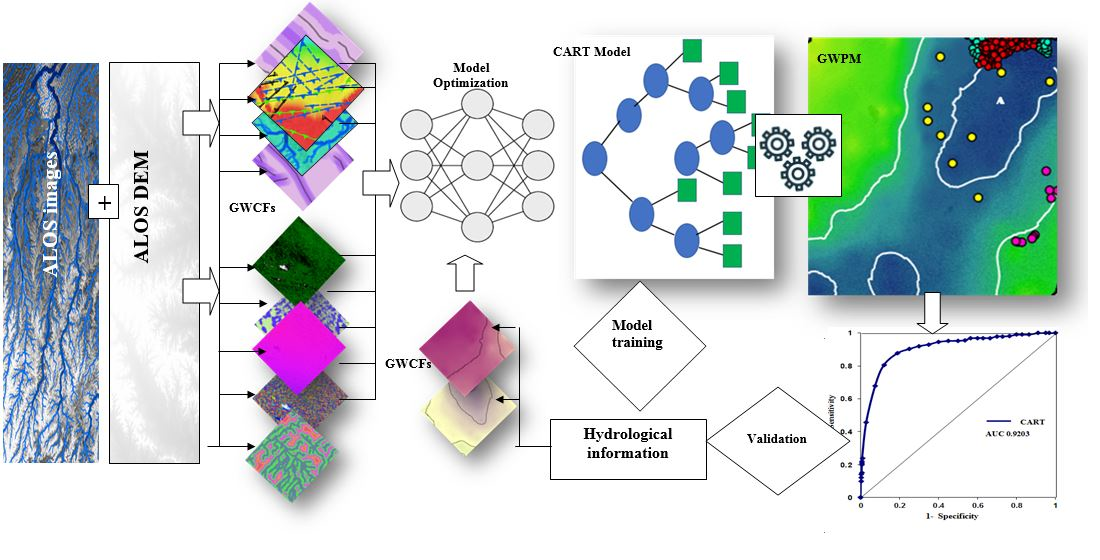
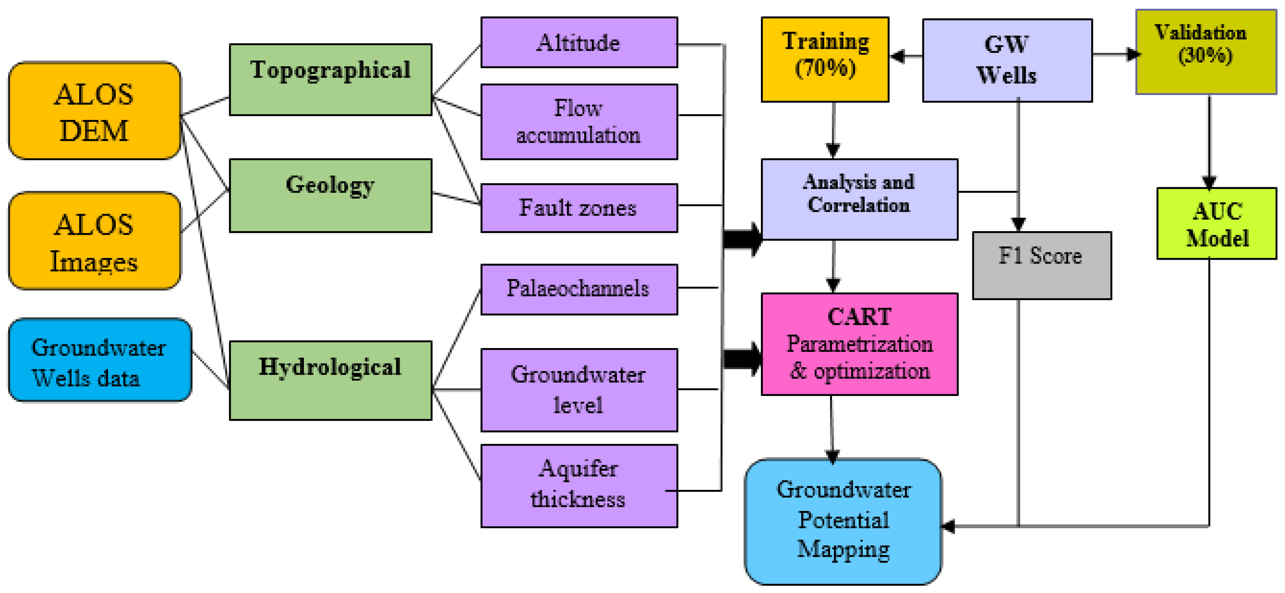
3. Materials and Methods

3.1. Materials and Preprocessing

Five datasets were used in this study. The first dataset was the digital elevation model (DEM) and images of the Phased Array type L-band Synthetic Aperture Radar (PALSAR) of the Advanced Land Observing Satellite (ALOS) with a spatial resolution of 30 m. The ALOS DEM and images were downloaded from the web page of the United States Geological Survey (USGS) (http://gdex.cr.usgs.gov/gdex/, accessed on 17 March 2021) and Japan Aerospace Exploration Agency, Earth Observation Research Center (https://www.eorc.jaxa.jp/ALOS/en/palsar_fnf/data/index.htm/, accessed on 17 March 2021).
We used this type of sensor owing to its ability to penetrate extremely dry sand sheets and imagine near-surface features over a regional scale with low-cost manners [55]. Additionally, the ALOS DEM has the lowest Root Mean Square Error (RMSE) than SRTM DEM [56]. These data were also chosen because it is difficult to create a precise DEM over a regional scale from a topographic map [57]. The second dataset was the SRTM DEM with a spatial resolution of 30 m and downloaded from the webpage of the United States Geologic Survey (USGS) (https://earthexplorer.usgs.gov/, accessed on 17 March 2021).
The third dataset was a collection of ancillary data, such as hydrological information collected from 150 oil groundwater wells drilled by Aramco tapping different rock and formations aquifers [2,31] and groundwater wells in the Oasis of Liwa, UAE, and a geologic map of the study area [40,41,42,43,58]. These datasets were used to construct maps of the aquifer thickness, groundwater table, groundwater quality and train and validate the CART model. A total of 185 groundwater well locations were mapped as points and randomly divided into 129 (70%) for training the model and 56 (30%) for validation [25,26]. Other hydrological information such as paleodelta, paleolake and lakes was also included to validate the resulting GWPM. The present study focuses on topography, hydrological and geology conditioning factors, which are extracted from the ALOS DEM and groundwater wells (Figure 4).

3.2. Construction of Groundwater Conditioning Factors

The most critical aspect in groundwater potential mapping is the selection of proper and suitable conditioning factors. These factors include terrain parameter, geology and hydrology that strongly influenced groundwater flow and accumulation. These factors were chosen based on their level of contribution to groundwater accumulation (Table 1). These major GWCFs can be exploited by the CART model to produce the optimal model [23,27]. Additionally, fault zones affect relief and often connected with valley networks or paleochannels and flow directions and accumulation. Terrain parameters can contribute to groundwater flow and accumulation as well as topographic wetness. Thus, terrain parameters such as altitude, slope, zones of flow accumulation were derived from the ALOS DEM using the raster surface tool implemented in ArcGIS v. 9.2 (Figure 4). In addition to topographic factors, geological structures and hydrological factors were also included. These factors were classified as continuous data such as altitude, slope and zones of flow accumulation and categorical data such as depth to basement. Unfortunately, lithologic and land use/land cover factors are not considered in this study because the ARAK area is characterized by low relief and covered by sand dunes. After that, all factors were regenerated in the ASCII grid format with a 30 m grid. Generally, the change in altitude reflects subsurface fault displacements. In turn, these fault zones control surface water and groundwater flow, landscape, topographic wetness and flow accumulation zones [1,52,53,54]. These faults were extracted using three data sets. First, a set of thematic maps such as altitude, slope, hill shade in all directions (0°, 45°, 90°, 135°, 270° and 315°) were derived from a DEM and faults were extracted based on the abruption change in the altitude map and tone change in shaded relief maps [6,7,8].
To validate the extracted fault zones, all faults were imported into a GIS environment. The validation was performed by draping faults extracted from remote sensing over the geological maps of the region constructed by Greet et al. (2001) [3], Sharland et al. (2001) [40], Johnson and Woldehaimanot (2003) [41] and Allen (2007) [42]. Finally, maps of fault density and distance from faults were calculated and reclassified using Euclidean and reclassify tools implemented in spatial analysis tools ArcGIS v. 9.2 software.
Paleochannels (wadi course) indicate flow direction and sources of recharge and discharge. Thus, surface and near-surface paleochannels were delineated from the ALOS DEM using a hydrological tool (D8 algorithm) implemented in ArcGIS v. 9. Mapping of paleochannels starts by filling the gaps in the DEM followed by producing flow along favoured directions agree with the slope direction (aspect) when it is a multiple of 45°, calculating the steepest slope and downhill slope of each central to one of eight neighbouring pixels and counting all the cells upstream of a proposed cell by the flow acculturation routine.
The major paleochannels were mapped and simulated by defining a threshold value of 400. After that, paleochannels were ordered into four-stream orders. We ordered paleochannels to indicate flooded and wet areas across the ARAK mega-basin. After that, all paleochannels based on flow direction derived from the ALOS DEM using ArcGIS v. 9.2 software. Finally, maps of distance from paleochannels and paleochannels density were calculated and reclassified using Euclidean, density and reclassify tools implemented in spatial analysis tools in ArcGIS v.9.2 software.
To validate the extracted paleochannels, the extracted paleochannels were imported into a GIS environment and draped over those from the Shuttle Radar topographic Mission (SRTM) and PALSAR images and visual inspection was performed by comparing their textural features evident in the Shuttle Radar topographic Mission (SRTM) with a spatial resolution of 30 m and PALSAR images [7,45]. The revealed features were also validated by comparing them with those mapped by Clarck (1989) [28], Dabbagh et al. (1997) [29] and Sultan et al. (2008) [31].

3.3. Analysis and Optimization of the GWCFs

After construction of all groundwater-related factors, it is important to assess the conditioning factors for optimizing and outliers and multi-collinearity issues [16]. The chi-square method was used to detect redundancy and optimize GWCFs. The chi-square statistic can be defined as a measure to quantify the degree of association between two maps. The calculations are based on the number from the area cross-tabulation. It measures the association of one map with another and describes it quantitatively. In this study, a spatial correlation between GWPM and each GWCF was measured. The measurement was performed as an area cross-tabulation, with classes of one map being, the rows, and the other classes of the second map being the columns.
The overall chi-square value represents the overall association between the groundwater wells map (Figure 1b) and each GWCF and the resulting GWPM. A higher value for chi-square indicates a more critical prediction factor and positive relationship between GWCGs and GW well locations. The p-value is assessed against the significant level of 0.05. This process can help to investigate if the CART model is enhancing or introduced a bias in the resulting GWPM.

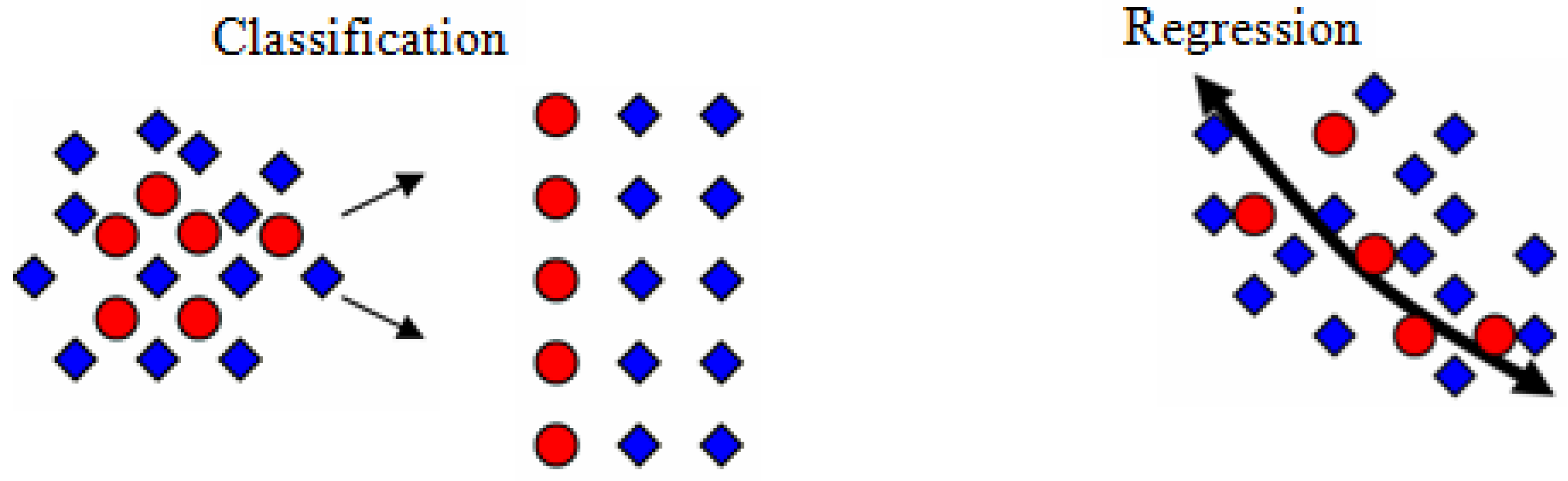
3.4. The Classification and Regression Trees (CART)

To map GWPM, it is important to employ a machine learning algorithm. The Classification and Regression Trees (CART) model is one of the most common algorithms for the classification of data [59]. It is resistant to miss data, and its variables do not need to have a normal distribution. The CART has been successfully applied in several applications such as photogrammetry [60], environmental protection [61], food science and chemistry [62,63], landslide susceptibility mapping [64,65,66], flash flood susceptibility mapping [67], and groundwater potential mapping [68,69].
The CART model is a binary recursive partitioning procedure capable of processing continuous and nominal attributes as targets and predictors and was developed by Friedman (1975) [70] and Breiman et al. (1984) [59]. The CART model is designed as a sequence of trees where the ends are terminal nodes. It comprises of three elements: (i) rules of splitting data at a node based on the value of one variable, (ii) stopping rules for deciding when a branch is terminal and can be split no more, and (iii) a prediction for the target variable in each terminal node (Figure 5).
At the first stage, classification is formed and leads to creating a tree with several branches. The number of branches of any tree depends on the degree of dispersion of data. The size of the tree depends on specific parameters such as the minimum population in the successive nodes, the minimum population of children, the maximum number of levels and the maximum number of nodes [59]. It is worth to not that there is no relationship between the size of the tree and the accuracy of classification.
The precise classification can be completed by reducing the overfitting of the training set. The stage of cutting is created by generating the biggest possible trees and this process lies in decreasing the total number of leaves and tending to increase the accuracy of classification. The final stage is the selection of a tree with a lower number of misclassifications and a higher accuracy. This higher accuracy can be released with the application of cross-validation using Equation (1):
RE (d) = 1/(N∑(i=1) (yi − d(xi))2
where yi is the number of points in the testing set (real variable), xi is the number of points in the testing set (variable classified with d model), N is the number of cases in a testing set. The results of the predicted model were evaluated using a set of testing samples. The measure of the cross-validation Ra(T) is a linear dependence between the complexity of the tree and the cost of misclassifications Equation (2) [59].
Rα (T) = R (T) + α T ↔ α = Rα (T) − R(T) / |T|
where Rα (T) is the cost-complexity measure, R(T) is the cost of misclassifications, |T| is the complexity of tree measures as the number of terminal nodes in the tree, a parameter of tree complexity (assumes values from 0 for a maximal tree to 1 for a minimal tree).

3.5. Application of the CART Model in Mapping Zones of Groundwater Potential

To map zones of groundwater potential, the GWCFs were converted into ASCII format in the ArcGIS environment. The related GWCFs were resampled into a 30 × 30 m grid format. After that, the CART model was fitted in STATISTICA v.7 [71] which widely used for regression classification associated with predicting continuous dependent variables [71]. After that, the CART model was trained using groundwater well locations, and optimal parametrization was performed. The optimal parameters were; the number of additive trees, learning rate and the proportion of sub-sampling. In this study, the optimal parameter values for additive trees were 186, the value for learning rate was 0.1, and the maximum size of the tree was five.
The chosen value may improve the accuracy of the results. Here, the random point’s values have been extracted from each groundwater conditioning factor (GWCF) for the absence and presence of the GWCF by running the CART. The related GWCFs were categorized into continuous and categorical data. The continuous data include topographic slope, topographic curvature, distance from the paleochannels, distance from the faults (Figure 6 and Figure 7).
The faults were classified as categorical data. During the process and prediction, the CART uses GWCFs, and the regression tree divides them into two groups [23,71]. A group in the upper part of the regression and another in the lower part of the regression. By using this classifier, zones of groundwater potentiality were calculated for each pixel in each GWCF. Finally, the produced GWP map was classified into five classes, namely very low, low, moderate, high and very high, using the natural break tool implemented in ArcGIS v. 9.2 software.

3.6. Validation

Locations of groundwater wells and discovered paleolakes and observed lakes are important hydrological information in the assessment and validation of the resulting of groundwater potential map (Elmahdy et al. 2020). This information was collected from groundwater wells, previous works and QuickBird images with a spatial resolution of 0.6m (Figure 2). Here, two validation methods were performed to validate the resulting GWPM. In the first method, all paleochannels and paleolakes by Edgell 2006 [34], Dabbagh, Al-Hinai, and Khan 1997 [29] and Clarck 1989 [28] as well as the observed lakes and paleodelta observed on Google Earth were imported into GIS environment and draped over the produced GWPM and visual comparison was performed. In the second method, the hydrological information (173 groundwater well and lake locations) was divided into 121 (70%) for the CART training and 52 (30%) for the CART validation using the Hawth’s Tool implemented in the ArcGIS v. 10.2 Software (Figure 1b).
The model validation was measured using the area under the curve (AUC) [72,73]. The AUC ranges from 0 to 1: AUC with a value of 1 indicating a good prediction, and a value of 0 indicating the model is not efficient and cannot predict GWP. Both the success and prediction rates were created to assess the accuracy of the GWPM [74]. The value of AUC can be estimated via the following equation [72,73]
AUC = S (TP + STN/(P + N))
where TP (true positive) and TN (true negative) are the numbers of pixels that are correctly classified. P is the total number of pixels with torrential phenomena, and N is the total number of pixels of no groundwater potential.
The ROC was used due to its simplicity, easiness and higher accuracy [64]. The curve has been successfully applied by several geoscience researchers in groundwater potential mapping [11,12,13], and land subsidence susceptibility mapping [23].

Evaluation Criteria

To evaluate the CART performance, standardized based on a pixel by pixel producing numerical values for GWP classes commission, classes omission, total of incorrect pixels, percentage of incorrect pixels, precession, recall, and F1 score [24]. These parameters were calculated based on true-positive (TP), true-negative (TN), false-positive (FP), and false-negative (FN). Accuracy, precision, recall and F1 score were calculated via the following Equations (4)–(8):
Accuracy =TP +( TN ̸ TP) +FP
Kappa = pope ̸̸̸ 1 − pe
where po is the observed agreement ratio and pe is the expected agreement.
Precision = TP/ TP + FP
Recall = TP ̸ TP + FN
F1 = 2 × precision × recall ̸ precision + recall
where TP is the true positive; FP is the false positive; and FN is the false negative.

4. Results

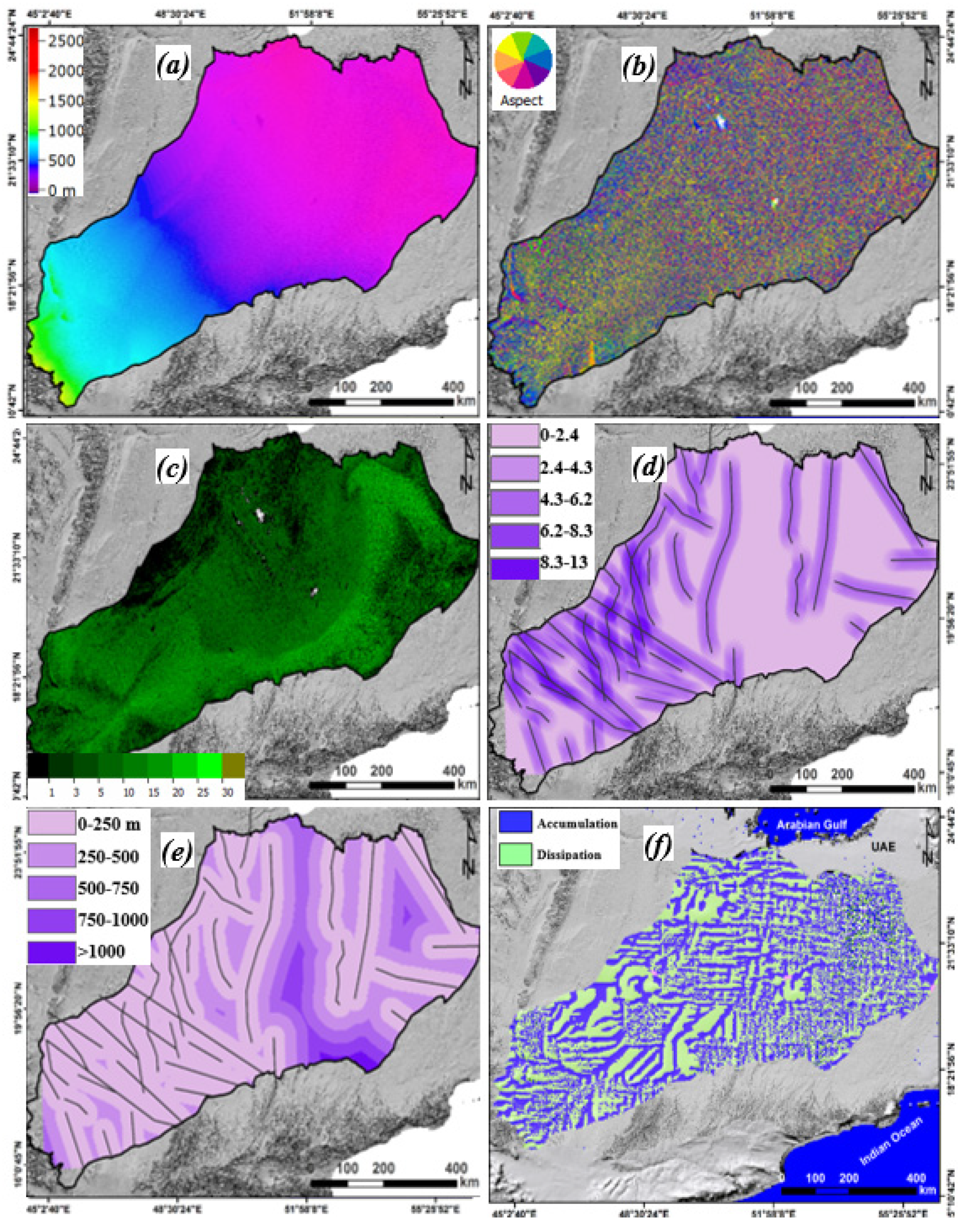
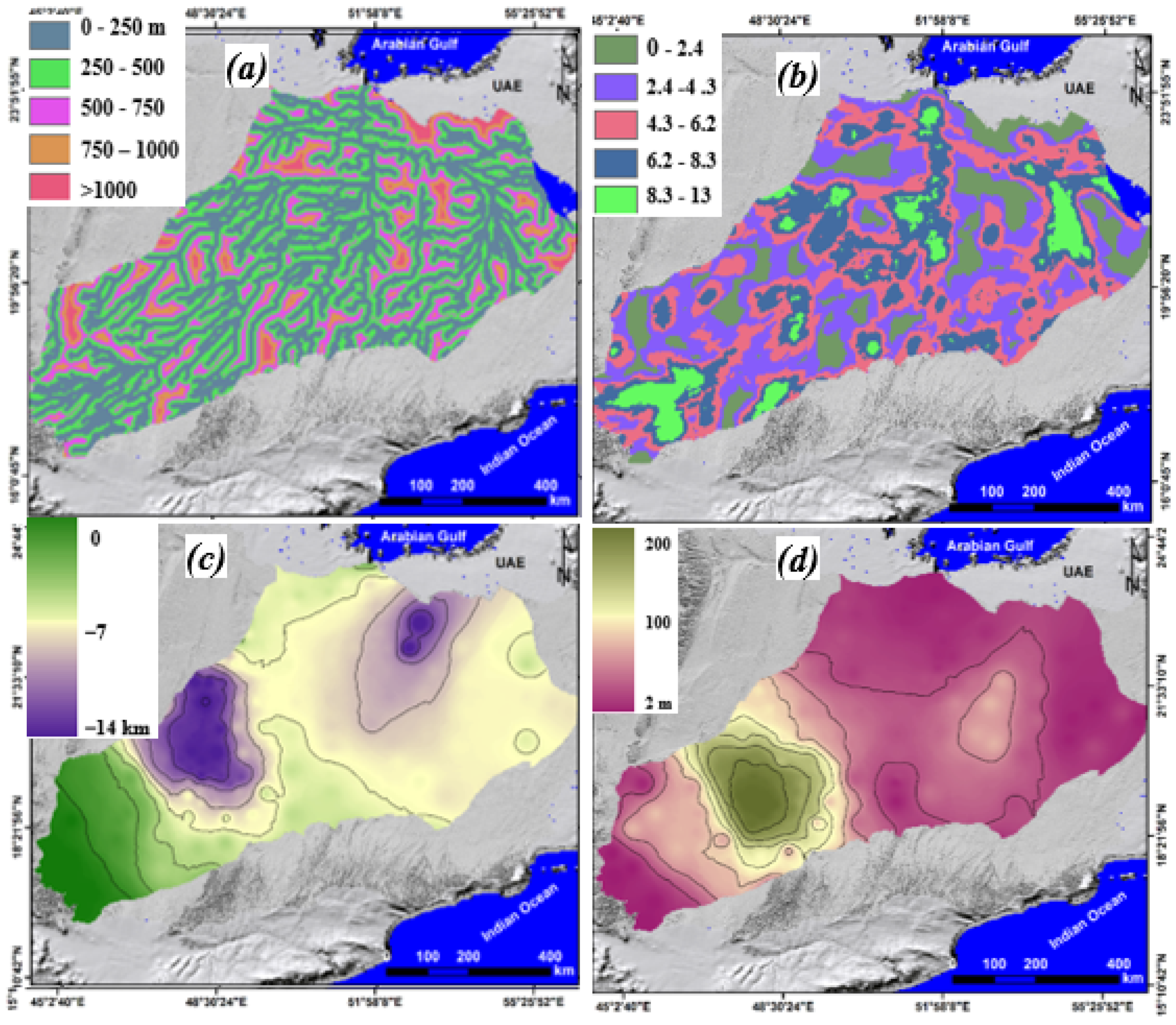
4.1. Spatial Analysis

In this study, chi-square was utilized to represent the spatial association and correlation between GWCFs and groundwater potential. According to Table 1, fault zones and faults density and their association paleochannels and zones of flow accumulation greater regional influence groundwater potential. These factors were observed the best GWCFs followed by altitude, paleochannels density, slope and distance from paleochannels. However, aspect and depth to the bed rock were observed the less significant for groundwater potential mapping in the ARAK area.

4.2. Groundwater Potential Mapping

The map of groundwater potential produced using the CART model is shown in Figure 8. The map shows that there are two zones of high and very high groundwater potentiality in the ARAK. The first zone is deep and located near the borders of Saudi Arabia and Yemen and Saudi Arabia and UAE borders like U in shape (dark blue colour in Figure 8), while the second zone is shallow and located near the borders of Saudi Arabia and Oman (green color in Figure 8).
The deep zone (sedimentary basin) extends from Ad Dawasir, Al Juf, Mondafan, Khujaymah and Sharourah near Saudi Arabia and Yemen borders to the SGSB, Shabita and Shieba near Saudi Arabia and UAE borders (Figure 1b and Figure 8). This zone covers an area of 256,235 km2 (45.2%) of the total area of the ARAK aquifer, which is estimated to be 566,838 km2. Ad Dawasir, Al Juf, Mondafan, Khujaymah and Sharourah areas received a considerable amount of water from Aseer and still receive an additional recharge [12]. The SGSB, Shabita, Shieba received their water via Harada in the east, Ad Dawasir and Al Juf tributaries in the west. We accordingly recovered a strong agreement between this zone and wells of high and very high productivity in Liwa, UAE (a in Figure 8) and the paleolakes in Mondafan and Khuaymah location (blue points in Figure 8).
Most of the high yield groundwater wells (yellow points in Figure 8) and the discovered paleolakes were observed to be located within a high density of paleochannels and fault zones, while the observed lakes were found to be located in the shallow depression of Mutaridah.
The shallow zone (macro-depression) is located in Saih Rawl, Mutaridah and Umm Al Hiesh, near the border with Saudi Arabia and Oman and occupies an area of about 66,223 km2. This zone received a considerable amount of water from three rechargeable sources in the mountains of Oman, Dhofar and Hadramout and still receive an additional recharge [12]. This zone appears as a mega-basin underneath sand sheets, as indicated by the presence of several lakes near the Umm Al Hash area (b in Figure 9) and paleodelta (c in Figure 9) recovered from Google Earth. As seen in Figure 6, this mega-basin (that is a macro-depression) is located at an elevation ranges from 85 to 120 m. The results are consistent with other studies [9,10,12,14,73] and revealed paleolakes and paleochannels from aerial photographs and SIR-C images by Clark (1989) [28] and Dabbagh et al. (1997) [29] (Figure 9d). According to local people, the groundwater of those lakes is rich in sulphur and more saline near Oman Saudi Arabia borders [12]. This may be due to the connection between the aquifers and fault zones which can serve as pathways for upward transport of deep-seated fossil water. In general, the ARAK received a considerable amount of water from the adjoining mountainous areas during the wet periods of the Late Quaternary and the intervening dry periods, as is the case now [12,14].
Fragaszy and McDonnell (2016) [73] investigated the hydrological unique of the Liwa Oasis, UAE and concluded that the groundwater wells productivity in the area is relatively high (20–50 m3/h) and very high (>50 m3/h) (Figure 9a). Crassard et al. (2013) [45] and Sultan et al. (2008) [12] concluded that groundwater table and groundwater quality in the ARAK area gradually decreases from Al Juf in the southwest to Mutaridah depression and the State of Qatar and UAE borders, including Shubaytah and Shaybah, in the northeast (Figure 9d and Figure 10). These areas have experienced significant evaporation, seawater intrusion, dissolution of carbonate rocks and salinization during dry seasons [2,12,14,73]. This salinization has led to increasing groundwater salinity which is directly proportional to δ18O in groundwater [72]. However, their deep aquifer has a higher probability of fresh fossil water as indicated by our results.

4.3. Validation

The CART model was validated using the ROC and the AUC was recalculated. The model exhibited an accuracy of 0.920, which represents a predictive accuracy of 92%. Thus, the validation confirmed a positive match between the reported groundwater well locations and zones predicted using the CART model (Figure 11). One of the main advantages of the CART model is that it is not extensively influenced by outliers in the used conditioning parameters [65,66,67,68,69]. Furthermore, it can employ the same conditioning parameters more than once in different parts of the tree. It incorporates both testing and cross-validation to evaluate the goodness of fit more precisely [23].
The results demonstrated that the CART model was able to map and predict zones of groundwater potential with an F1 score ranging from 0.94-1 (Figure 12). In particular, the values of F1 score, precision and recall for high and very high zones are quite higher than moderate (0.9) and low zones (0.88) across the CART model. Very low zone showed the lowest values (<0.80) for precision, recall, and F1. The CART model demonstrated ability in discriminating between zones of high and low groundwater potential. High and very high potential mapped by the CART has a wider range compared with zones of low and very low potential. The CART model is flexible and more suitable for a wide range of mapping and predicting problems [23].
Qualitative assessment of the resulting GWPM with the result of Fragaszy and McDonnell (2016) [73], Clark (1989) [28], and Dabbagh et al. (1997) [29] (Figure 9d) generally correlates. Thus, we assume that the GWPM obtained (Figure 8) is rather realistic.

5. Discussion

5.1. Spatial Analysis

Unlike other optimizer methods, the chi-square optimizer is able to categorize GWCFs based on their level of contribution to groundwater potential [72]. The results of the optimization depend on the scale and relief of the study area and the number of GWCFs [23]. The results of spatial analysis and correlation showed that factors such as faults and their associations paleochannels and zones of flow accumulation have a very strong influence on groundwater potential, especially in remote arid and semi-arid regions. However, the result appeared to suggest that factors such as aspect and depth to the basement not have a significant level of contribution to groundwater potential. This result is in agreement with another study [14]. Fault zone intersections and fractures are significant features of the groundwater aquifers and the Earth’s crust [54]. These features improve the effective porosity and permeability of the aquifer and abnormally high discharges of springs and groundwater wells [12,52,53]. They affect relief, altitude and landscape that control water flow and accumulation [52,53]. These features control the spatial distribution of paleochannels, zones of flow accumulation [52,53,75]. So, paleochannels, slope and zones of flow accumulation have a higher value for Chi-square after fault zones. Depth to groundwater has a moderate value for Chi-square. There is no surprise since fault zones are often connected with paleochannels and control altitude, slope zones of flow accumulation. Unfortunately, we cannot consider GWCFs such as LULC, lithology and plan curvature have not considered because the region is remote and inaccessible, and the terrain is characterized by a gentle slope covered by sand sheets. In such regions, the use of several GWCFs such as plan curvature, aspect, and LULC may not much affect the results and introduces errors [14,23]. Ozdemir [29,30] exhibited that the lineaments and stream density-related factors had a positive correlation with groundwater potential, while the slope shows a negative correlation.

5.2. The CART Application

In this paper, we applied the CART model to map zones of groundwater potential in an arid region over a very regional scale using a few GWCFs for the first time. These GWCFs include new detailed maps such as paleochannels and zone of flow accumulation. Unfortunately, we cannot conduct a field validation of the resulting maps due to its harsh weather, remote location and lack of rock outcrops [2,3].
We can carry out a comparison of the resulting map (Figure 8) with groundwater well with high yield (yellow points in Figure 8), zones of high and very high productivity in Liwa oasis, UAE [73] (A in Figure 8 and Figure 9a), observed lakes and paleodelta (Figure 9b,c) and paleochannels and Mutaridah depression revealed from aerial photographs and SIR-C images by Clark (1989) [28] and Dabbagh et al. (1997) [29] (Figure 9d). These features are exactly localized on the zone of high and very high potential in the resulting GWPM (Figure 9). This is due to we used similar remote sensing and hydrological data with similar spatial resolution. Further validation using the ROC and the AUC exhibited an accuracy of 0.920, which represents a predictive accuracy of 92%. This value is greatly affected by overfitting and underfitting. This is because overfitting and underfitting are not randomly distributed [66]. In fact, this result highlights a significant decrease of bias and errors through the CART model. This result is in agreement with Elmahdy et al. [23] and Aguiar et al. [27] in which the CART model can reinforce the accuracy of prediction.
Comparing to other machine learning algorithms such as Random Forest (RF) and Boosted Regression Trees (BRT), the CART model showed the highest accuracy [63,69]. The CART, as a classifier, is suitable for numeric data types and generates an invariant for the transformation of independent variables [27,32]. The result showed that the accuracy of the resulting map depends on the precision of the GWCFs and the scale of the study area. This result agrees well with Elmahdy et al. (2020d) [23] and Elmahdy et al. (2020a) [26], who found a positive relationship between the scale and the accuracy of the predicted map. The CART model has been successfully applied to predict pulmonary tuberculosis in hospitalized patients with an accuracy of 79.70% [27].
Pham et al. (2018) [65] concluded that the performance of the CART algorithm is much better than the logistic regression (LR) model. The CART model showed more application than other decision tree models [74]. However, the Kernel Logistic Regression (KLR) model is better than the CART model [66]. So, we assume that the resulting GWPM is somewhat realistic. However, the CART model had some overfitting problems. These problems may be related to poor generalization from training datasets and increased errors for real data. To reduce overfitting, we increased training and change the complexity of the model. Change complexity was performed by changing the network structure (numbers of weight) and parameters (values of the weight) of the model. In this study, the GWCFs used still encompassed small errors and noise. This is because the classes of high and very high groundwater potential are quite similar to those of low and very low groundwater potential.
The results obtained (Figure 8) demonstrate that new maps of paleochannels, flow accumulation zones and GWPM can be used to improve water resources plans and groundwater exploration in an arid region over a very regional scale.
Future work will be carried out to compare the performance of the CART model against random forest (RF) using similar GWCFs. The new maps and the CART model are helpful for water resources and hydrological specialists and a better understanding of the hydrological setting of the ARAK aquifer underneath sand sheets.

6. Conclusions

This study presents the classification and regression trees (CART) model (as an application) to map zones of groundwater potential over a regional scale over a regional scale for the first time with a moderate number of GWCFs. The CART model was chosen based on several studies applied to compare the performance of the CART model against other algorithm applications in the landslides, flash floods and pulmonary tuberculosis in hospitalized patients’ prediction. Different GWCFs have been constructed and used for GWP mapping and investigate the ability of the CART in prediction over a very regional scale with a moderate number of GWCFs. These GWCFs include altitude, aspect, slope, distance from faults, distance from paleochannels, fault density, paleochannels density, flow accumulation zones, depth to basement and groundwater table in conjunction with 185 GW wells for training and validation. The best groundwater potential conditioning factors were fault zones and fault density as they control paleochannels, flow accumulation zones, slope and depth to basement. However, we did not observe any level of contribution of aspect to GWP. Additionally, we cannot generate GWCFs such as plan curvature and land use/ land cover due to the low relief and aridity of the region. These factors are the most suitable for groundwater potential mapping in an arid region covered with sand sheets and may differ from those for mapping in tropical regions. The results reveal that the CART performs well in terrain covered with sand sheets using a moderate number of GWCFs. The CART produced a predictive accuracy of 92%.
Two zones of a higher probability of groundwater potential were mapped using the CART model. The first zone is located in Mundafan, Kujaymah and Wajid near Saudi Arabia and Yemen borders and reserve freshwater. The second zone is located in Shubayta, Shaiba and Mutaridah near Oman, Saudi Arabia and UAE borders. These two zones are the hope of the Arabian Gulf council Countries (AGCC), especially Saudi Arabia and the United Arab Emirates (UAE).
The GWCFs and the CART applied in this study could be applicable to map groundwater potential over a regional scale in similar regions such as the Arabian Sahara in Egypt and Libya. These results greatly help geologists and hydrologists recommend zones for groundwater exploration and fill an important gap between hydrological, geological and paleoenvironmental understanding of the largest and most inaccessible aquifer in the world.

Author Contributions

S.E.: Conceptualization; Data curation; Formal analysis; Investigation; Methodology; Software; Validation; Visualization; Writing—original draft; T.A.: Funding acquisition; Methodology; Project administration; Supervision; Writing—review & editing; M.M.: Funding acquisition; Methodology; Resources; Writing—review & editing. All authors have read and agreed to the published version of the manuscript.

Funding

The research has received funding under financial grant SCRI 18 Grant EN0- 284 and the national water and energy center, United Arab Emirates University through the Asian University Alliance (AUA) program, grants number 31R281-AUA-NWEC-4-2020 and 12R023-AUA-NWEC-4-2020.

Conflicts of Interest

The authors declare no conflict of interest.

References

  1. Elmahdy, S.I.; Mohamed, M.M. Remote sensing and GIS applications of surface and near-surface hydromorphological features in Darfur region, Sudan. Int. J. Remote Sens. 2013, 34, 4715–4735. [Google Scholar] [CrossRef]
  2. Dimock, W.C. A Study of the Water Resources of the Rub Al-Khali in Southern Saudi Arabia; ARAMCO: Ryadh, Saudi Arabia, 1961; p. 183, Unpublished Groundwater Report 22. [Google Scholar]
  3. Geert, K.; Afifi, A.M.; Al-Hajri, S.I.A.; Droste, H.J. Paleozoic stratigraphy and hydrocarbon habitat of the Arabian Plate. GeoArabia 2001, 6, 407–442. [Google Scholar]
  4. Pachur, H.-J.; Rottinger, F. Evidence for a large extended paleolake in the Eastern Sahara as revealed by spaceborne radar lab images. Remote Sens. Environ. 1997, 61, 437–440. [Google Scholar] [CrossRef]
  5. Hoelzmann, P.; Keding, B.; Berke, H.; Kröpelin, S.; Kruse, H.J. Environmental change and archaeology: Lake evolution and human occupation in the Eastern Sahara during the Holocene. Palaeogeogr. Palaeoclimatol. Palaeoecol. 2001, 169, 193–217. [Google Scholar] [CrossRef]
  6. Elmahdy, S.I.; Mohamed, M.M. Remote sensing and geophysical survey applications for delineating near-surface palaeochannels and shallow aquifer in the United Arab Emirates. Geocarto Int. 2015, 30, 723–736. [Google Scholar] [CrossRef]
  7. Elmahdy, S.I.; Mohamed, M.M. Mapping of tecto-lineaments and investigate their association with earthquakes in Egypt: A hybrid approach using remote sensing data. Geomat. Nat. Hazards Risk 2015, 7, 600–619. [Google Scholar] [CrossRef] [Green Version]
  8. Elmahdy, S.I.; Mohamed, M.M. Relationship between geological structures and groundwater flow and groundwater salinity in Al Jaaw Plain, United Arab Emirates; mapping and analysis by means of remote sensing and GIS. Arab. J. Geosci. 2013, 7, 1249–1259. [Google Scholar] [CrossRef]
  9. Clark, A. Lakes of the Rub’ Al-Khali. Aramco World 1989, 40, 28–33. [Google Scholar]
  10. Dabbagh, A.E.; Al-Hinai, K.G.; Khan, M.A. Detection of sand-covered geologic features in the Arabian Peninsula using SIR-C/X-SAR data. Remote Sens. Environ. 1997, 59, 375–382. [Google Scholar] [CrossRef]
  11. Elmahdy, S.I. Hydromorphological mapping and analysis for characterizing darfur paleolake, NW Sudan using remote sensing and GIS. Int. J. Geosci. 2012, 3, 25. [Google Scholar] [CrossRef] [Green Version]
  12. Sultan, M.; Sturchio, N.; Al Sefry, S.; Milewski, A.; Becker, R.; Nasr, I.; Sagintayev, Z. Geochemical, isotopic, and remote sensing constraints on the origin and evolution of the Rub Al Khali aquifer system, Arabian Peninsula. J. Hydrol. 2008, 356, 70–83. [Google Scholar] [CrossRef]
  13. Moghaddam, D.; Rezaei, M.; Pourghasemi, H.R.; Pourtaghie, Z.S.; Pradhan, B. Groundwater spring potential mapping using bivariate statisticalmodel and GIS in the Taleghan watershed, Iran. Arabian J. Geosci. 2015, 8, 913–929. [Google Scholar] [CrossRef]
  14. Mohamed, M.M.; Elmahdy, S.I. Remote sensing and information value (IV) model for regional mapping of fluvial channels and topographic wetness in the Saudi Arabia. GISci. Remote Sens. 2016, 53, 520–541. [Google Scholar] [CrossRef]
  15. Stumpf, A.; Kerle, N. Object-oriented mapping of landslides using Random Forests. Remote Sens. Environ. 2011, 115, 2564–2577. [Google Scholar] [CrossRef]
  16. Stumpf, A.; Kerle, N. Combining Random Forests and object-oriented analysis for landslide mapping from very high-resolution imagery. Procedia Environ. Sci. 2011, 3, 123–129. [Google Scholar] [CrossRef] [Green Version]
  17. Vorpahl, P.; Elsenbeer, H.; Maerker, M.; Schröder, B. How can statistical models help to determine driving factors of landslides? Ecol. Model. 2012, 239, 27–39. [Google Scholar] [CrossRef]
  18. Trigila, A.; Frattini, P.; Casagli, N.; Catani, F.; Crosta, G.; Esposito, C.; Iadanza, C.; Lagomarsino, D.; Mugnozza, G.S.; Segoni, S.; et al. Landslide Susceptibility Mapping at National Scale: The Italian Case Study. Landslide Sci. Pract. 2013, 1, 287–295. [Google Scholar] [CrossRef] [Green Version]
  19. Demšar, U. Knowledge Discovery in the Environmental Sciences: Visual and Automatic Data Mining for Radon Problems in Groundwater. Trans. GIS 2007, 11, 255–281. [Google Scholar] [CrossRef]
  20. Baudron, P.; Alonso-Sarría, F.; García-Aróstegui, J.-L.; Cánovas-García, F.; Martínez-Vicente, D.; Moreno-Brotóns, J. Identifying the origin of groundwater samples in a multi-layer aquifer system with Random Forest classification. J. Hydrol. 2013, 499, 303–315. [Google Scholar] [CrossRef]
  21. Rodriguez-Galiano, V.; Mendes, M.P.; Garcia-Soldado, M.J.; Olmo, M.C.; Ribeiro, L. Predictive modeling of groundwater nitrate pollution using Random Forest and multisource variables related to intrinsic and specific vulnerability: A case study in an agricultural setting (Southern Spain). Sci. Total. Environ. 2014, 476–477, 189–206. [Google Scholar] [CrossRef]
  22. Elmahdy, S.I.; Mohamed, M.M.; Ali, T.A. Automated detection of lineaments express geological linear features of a tropical region using topographic fabric grain algorithm and the SRTM DEM. Geocarto Int. 2021, 36, 76–95. [Google Scholar] [CrossRef]
  23. Elmahdy, S.; Ali, T.; Mohamed, M. Flash Flood Susceptibility Modeling and Magnitude Index Using Machine Learning and Geohydrological Models: A Modified Hybrid Approach. Remote Sens. 2020, 12, 2695. [Google Scholar] [CrossRef]
  24. Elmahdy, S.I.; Ali, T.A.; Mohamed, M.M.; Howari, F.M.; Abouleish, M.; Simonet, D. Spatiotemporal Mapping and Monitoring of Mangrove Forests Changes From 1990 to 2019 in the Northern Emirates, UAE Using Random Forest, Kernel Logistic Regression and Naive Bayes Tree Models. Front. Environ. Sci. 2020, 8, 102. [Google Scholar] [CrossRef]
  25. Elmahdy, S.; Mohamed, M.; Ali, T. Land Use/Land Cover Changes Impact on Groundwater Level and Quality in the Northern Part of the United Arab Emirates. Remote Sens. 2020, 12, 1715. [Google Scholar] [CrossRef]
  26. Elmahdy, S.I.; Mohamed, M.M.; Ali, T.A.; Abdalla, J.E.-D.; Abouleish, M. Land subsidence and sinkholes susceptibility mapping and analysis using random forest and frequency ratio models in Al Ain, UAE. Geocarto Int. 2020, 1–17. [Google Scholar] [CrossRef]
  27. Aguiar, F.S.; Almeida, L.L.; Ruffino-Netto, A.; Kritski, A.L.; Mello, F.C.; Werneck, G.L. Classification and regression tree (CART) model to predict pulmonary tuberculosis in hospitalized patients. BMC Pulm. Med. 2012, 12, 40. [Google Scholar] [CrossRef] [PubMed]
  28. Dixon, B. A case study using SVM, NN and logistic regression in a GIS to predict wells contaminated with Nitrate-N. Hydrogeol. J. 2009, 17, 1507–1520. [Google Scholar] [CrossRef]
  29. Ozdemir, A. GIS-based groundwater spring potential mapping in the Sultan Mountains (Konya, Turkey) using frequency ratio, weights of evidence and logistic regression methods and their comparison. J. Hydrol. 2011, 411, 290–308. [Google Scholar] [CrossRef]
  30. Ozdemir, A. Using a binary logistic regression method and GIS for evaluating and mapping the groundwater spring potential in the Sultan Mountains (Aksehir, Turkey). J. Hydrol. 2011, 405, 123–136. [Google Scholar] [CrossRef]
  31. Manap, M.A.; Nampak, H.; Pradhan, B.; Lee, S.; Sulaiman, W.N.A.; Ramli, M.F. Application of probabilistic-based frequency ratio model in groundwater potential mapping using remote sensing data and GIS. Arab. J. Geosci. 2014, 7, 711–724. [Google Scholar] [CrossRef]
  32. Breiman, L.; Friedman, J.H.; Olshen, R.A.; Stone, C.J. Classification and Regression Trees; Wadsworth: Belmont, CA, USA, 2017. [Google Scholar]
  33. Holm, D.A. Desert Geomorphology in the Arabian Peninsula. Science 1960, 132, 1369–1379. [Google Scholar] [CrossRef]
  34. Edgell, H.S. Arabian Deserts: Nature, Origin and Evolution; Springer Science & Business Media: Berlin, Germany, 2006. [Google Scholar]
  35. Petraglia, M.D.; Alsharekh, A.; Breeze, P.; Clarkson, C.; Crassard, R. Hominin Dispersal into the Nefud Desert and Middle Palaeolithic Settlement along the Jubbah Palaeolake, Northern Arabia. PLoS ONE 2012, 7, e49840. [Google Scholar] [CrossRef]
  36. Patlakas, P.; Stathopoulos, C.; Flocas, H.; Kalogeri, C.; Kallos, G. Regional Climatic Features of the Arabian Peninsula. Atmosphere 2019, 10, 220. [Google Scholar] [CrossRef] [Green Version]
  37. Woods, W.W.; Imes, J.L. How wet is wet? Precipitation constraints on late quaternary climate in the southern Arabian Peninsula. J. Hydrol. 1995, 164, 263–268. [Google Scholar] [CrossRef]
  38. Haynes, C.V. Oyo a Lost Oasis of the Southern Libyan Desert. Geograph. J. 1989, 155, 189–195. [Google Scholar] [CrossRef]
  39. Elmahdy, S.; Ali, T.; Mohamed, M. Hydrological modeling of Ar Rub Al Khali, Arabian Peninsula: A modified remote sensing approach based on the weight of hydrological evidence. Geocarto Int. 2021, 1–20. [Google Scholar] [CrossRef]
  40. Sharland, P.R.; Archer, R.; Casey, D.M.; Davies, R.B.; Hall, S.H.; Heward, A.P.; Horbury, A.D.; Simmons, M.D. Arabian Plate sequence stratigraphy. GeoArabia Spec. Publ. 2001, 2, 371. [Google Scholar]
  41. Johnson, P.R.; Woldehaimanot, B. Development of the Arabian-Nubian Shield: Perspectives on accretion and de-formation in the northern East African Orogen and the assembly of Gondwana. Geol. Soc. Lond. Spec. Publ. 2003, 206, 289–325. [Google Scholar] [CrossRef]
  42. Allen, P.A. The Huqf Supergroup of Oman: Basin development and context for Neoproterozoic glaciation. Earth Sci. Rev. 2007, 84, 139–185. [Google Scholar] [CrossRef]
  43. Stoeser, D.B.; Frost, C.D. Nd, Pb, Sr, and O isotopic characterization of Saudi Arabian Shield terranes. Chem. Geol. 2006, 226, 163–188. [Google Scholar] [CrossRef]
  44. Rosenberg, T.M.; Preusser, F.; Blechschmidt, I.; Fleitmann, D.; Jagher, R.; Matter, A. Late Pleistocene palaeolake in the interior of Oman: A potential key area for the dispersal of anatomically modern humans out-of-Africa? J. Quat. Sci. 2012, 27, 13–16. [Google Scholar] [CrossRef]
  45. Crassard, R.; Petraglia, M.D.; Drake, N.A.; Breeze, P.; Gratuze, B.; Alsharekh, A.; Robin, C.J. Middle Palaeolithic and Ne-olithic occupations around Mundafan palaeolake, Saudi Arabia: Implications for climate change and human dispersals. PLoS ONE 2013, 8, e69665. [Google Scholar] [CrossRef] [PubMed]
  46. Groucutt, H.S.; White, T.S.; Clark-Balzan, L.; Parton, A.; Crassard, R.; Shipton, C.; Alsharekh, A. Human occupation of the Arabian empty quarter during MIS 5: Evidence from Mundafan Al-Buhayrah, Saudi Arabia. Quat. Sci. Rev. 2015, 119, 116–135. [Google Scholar] [CrossRef]
  47. Pike, J.G. The evaporation of grondwater from coastal Playas in the Arabian Gulf. J. Hydrol. 1971, 2, 10–18. [Google Scholar]
  48. Mohamed, M.M.; Elmahdy, S.I. Fuzzy logic and multi-criteria methods for groundwater potentiality mapping at Al Fo’ah area, the United Arab Emirates (UAE): An integrated approach. Geocarto Int. 2017, 32, 1120–1138. [Google Scholar] [CrossRef]
  49. McClure, H. Early paleozoic glaciation in Arabia. Palaeogeogr. Palaeoclim. Palaeoecol. 1978, 25, 315–326. [Google Scholar] [CrossRef]
  50. Dyer, R.A.; Husseini, M. The Western Rub’Al-Khali Infracambrian Graben System. In Middle East Oil Show; Society of Petroleum Engineers: Manama, Bahrain, 1991. [Google Scholar]
  51. Wender, L.E.; Bryant, J.W.; Dickens, M.F.; Neville, A.S.; Al-Moqbel, A.M. Paleozoic Pre-Khuff Hydrocarbon Geology of the Ghawar Area, Eastern Saudi Arabia. GeoArabia 1998, 3, 273–302. [Google Scholar]
  52. Florinsky, I.V. Relationships between topographically expressed zones of flow accumulation and sites of fault intersection: Analysis by means of digital terrain modelling. Environ. Model. Softw. 2000, 15, 87–100. [Google Scholar] [CrossRef]
  53. Elmahdy, S.I.; Mohamed, M.M. Influence of geological structures on groundwater accumulation and groundwater salinity in Musandam Peninsula, UAE and Oman. Geocarto Int. 2013, 28, 453–472. [Google Scholar] [CrossRef]
  54. Poletaev, A.I. Fault Intersections of the Earth Crust; Geoinformmark: Moscow, Russia, 1992. [Google Scholar]
  55. Roth, L.; Elachi, C. Coherent electromagnetic losses by scattering from volume inhomogeneities. IRE Trans. Antennas Propag. 1975, 23, 674–675. [Google Scholar] [CrossRef]
  56. Santillan, J.R.; Makinano-Santillan, M. Vertical accuracy assessment of 30-M Resolution ALOS, ASTER, and SRTM global dems over northeastern Mindano, Philippines. Int. Arch. Photogramm. Remote Sens. Spat. Inf. Sci. 2016, 41, 33–37. [Google Scholar]
  57. Jarvis, A.; Rubiano, J.; Nelson, A.; Farrow, A. Practical Use of SRTM Data in the Tropics: Comparisons with Digital Elevation Models Generated Cartographic Data; International Center for Tropical Agriculture: Cali, Colombia, 2004. [Google Scholar]
  58. Stern, J.R.; Johnson, P. Continental lithosphere of the Arabian Plate: A geologic, petrologic, and geophysical synthesis. Earth-Sci. Rev. 2010, 101, 29–67. [Google Scholar] [CrossRef]
  59. Breiman, L.; Jerome, F.; Charles, J.S.; Richard, A.O. Classification and Regression Trees; Wadsworth Int. Group: Dordrecht, The Netherlands, 1984; Volume 37, pp. 237–251. [Google Scholar]
  60. Belgiu, M.; Drăguţ, L. Random forest in remote sensing: A review of applications and future directions. ISPRS J. Photogramm. Remote Sens. 2016, 114, 24–31. [Google Scholar] [CrossRef]
  61. Bel, L.; Allard, D.; Laurent, J.M.; Cheddadi, R.; Bar-Hen, A. CART algorithm for spatial data: Application to environmental and ecological data. Comput. Stat. Data Anal. 2009, 53, 3082–3093. [Google Scholar] [CrossRef]
  62. Chen, X.; Wang, L.; Qu, J.; Guan, N.-N.; Li, J.-Q. Predicting miRNA–disease association based on inductive matrix completion. Bioinformatics 2018, 34, 4256–4265. [Google Scholar] [CrossRef]
  63. Gregor, J.; Garrett, N.; Gilpin, B.; Randall, C.; Saunders, D. Use of classification and regression tree (CART) analysis with chemical faecal indicators to determine sources of contamination. N. Z. J. Mar. Freshw. Res. 2002, 36, 387–398. [Google Scholar] [CrossRef]
  64. Kamp, U.; Growley, B.J.; Khattak, G.A.; Owen, L. GIS-based landslide susceptibility mapping for the 2005 Kashmir earthquake region. Geomorphology 2008, 101, 631–642. [Google Scholar] [CrossRef]
  65. Pham, B.T.; Prakash, I. Machine Learning Methods of Kernel Logistic Regression and Classification and Regression Trees for Landslide Susceptibility Assessment at Part of Himalayan Area, India. Indian J. Sci. Technol. 2018, 11, 1–10. [Google Scholar] [CrossRef] [Green Version]
  66. Pham, B.T.; Prakash, I.; Bui, D.T. Spatial prediction of landslides using a hybrid machine learning approach based on Random Subspace and Classification and Regression Trees. Geomorphology 2018, 303, 256–270. [Google Scholar] [CrossRef]
  67. Band, S.S.; Janizadeh, S.; Pal, C.S.; Saha, A.; Chakrabortty, R.; Melesse, A.M.; Mosavi, A. Flash Flood Suscep-tibility Modeling Using New Approaches of Hybrid and Ensemble Tree-Based Machine Learning Algorithms. Remote Sens. 2020, 12, 3568. [Google Scholar] [CrossRef]
  68. Duan, H.; Deng, Z.; Deng, F.; Wang, D. Assessment of Groundwater Potential Based on Multicriteria Decision Making Model and Decision Tree Algorithms. Math. Probl. Eng. 2016, 2016, 2064575. [Google Scholar] [CrossRef] [Green Version]
  69. Nguyen, P.T.; Ha, D.H.; Jaafari, A.; Nguyen, H.D.; Van Phong, T.; Al-Ansari, N.; Prakash, I.; Van Le, H.; Pham, B.T. Groundwater Potential Mapping Combining Artificial Neural Network and Real AdaBoost Ensemble Technique: The DakNong Province Case-study, Vietnam. Int. J. Environ. Res. Public Health 2020, 17, 2473. [Google Scholar] [CrossRef] [PubMed] [Green Version]
  70. Friedman, L.A. The Measure of a Successful Information Storage and Retrieval System. In Perspectives in Information Science; Springer: Dordrect, The Netherlands, 1975; pp. 379–408. [Google Scholar]
  71. StatSoft. STATISTICA Data Miner: Integrating R Programs into the Data Miner Environment; StatSoft Business White Paper; GeoSoft, Inc.: Tusla, OK, USA; New York, NY, USA, 2003. [Google Scholar]
  72. Elmahdy, S.I.; Mohamed, M.M. Groundwater of Abu Dhabi Emirate: A regional assessment by means of remote sensing and geographic information system. Arabian J. Geosci. 2015, 8, 11279–11292. [Google Scholar] [CrossRef]
  73. Fragaszy, S.; McDonnell, R. Oasis at a Crossroads: Agriculture and Groundwater in Liwa, United Arab Emirates. IWMI Project Publication: Groundwater Governance in the Arab World–Taking Stock and Addressing the Challenges; USAID: Washington, DC, USA, 2016. [Google Scholar]
  74. Lin, N.; Noe, D.; He, X. Tree-Based Methods and Their Applications. In Springer Handbook of Engineering Statistics; Springer Science and Business Media LLC: London, UK, 2006; pp. 551–570. [Google Scholar]
  75. Ollier, C. Tectonics and Landforms; Longman: London, UK, 1981. [Google Scholar]
Figure 1. Maps of the Arabian Peninsula (a), and RGB 652 band combination of Landsat image of Ar Rub Al Khali mega-basin (black polygon) and Ar Rub Al Khali (ARAK) aquifer underneath sand sheets (red polygon) (b), red and black points highlight city and groundwater well locations, respectively. Green points highlight locations of the discovered paleolakes [2,3].
Remotesensing 13 02300 g001
Figure 2. Maps of rainfall (a) and geology (b) showing the spatial distribution of precipitation and lithological and structural units across the ARAK mega-basin [2,3].
Remotesensing 13 02300 g002
Figure 3. E–W regional geological cross-section across the ARAK region constructed from oil wells showing how the Oman Mountain and sedimentary groups formed and deformed, including the hydrological aquifers in the study area [2,3].
Remotesensing 13 02300 g003
Figure 4. Flowchart of the methodology.
Remotesensing 13 02300 g004
Figure 5. Diagrams represent Classification and Regression Trees (CART).
Remotesensing 13 02300 g005
Figure 6. Maps of altitude (a), aspect (b), slope (c) fault density (d), distance from faults (e), and zones of flow accumulation for the ARAK.
Remotesensing 13 02300 g006
Figure 7. Maps of distance from paleochannels (a), paleochannels density (b), depth to basement (c), and groundwater table (d) for the ARAK aquifer.
Remotesensing 13 02300 g007
Figure 8. Map of groundwater potentiality of the ARAK underneath sand sheets produced using the CART model. Pink points highlight recovered palaleolake locations and A, B and C point locations used for validation of the resulting GWPM.
Remotesensing 13 02300 g008
Figure 9. Maps of zones of high and very productivity in Liwa oasis (a) mapped using groundwater data by Fragaszy and McDonnell (2016) [73], recovered lakes (b) and paleodelta (c), and paleochannels and Mutridah depression mapped from SIR-C image using screen digitizing by clarck (1989) [9] (d).
Remotesensing 13 02300 g009
Figure 10. Interpolated map of the total dissolved solids (TDS) showing the gradual decrease of groundwater quality in the study area.
Remotesensing 13 02300 g010
Figure 11. ROC curve for groundwater potentiality map produced the CART and area under curve (AUC).
Remotesensing 13 02300 g011
Figure 12. F1, precision, and recall scores for the groundwater potential zones mapped using the CART model.
Remotesensing 13 02300 g012
Table 1. Importance of each GWCF calculated using chi-square method.
FactorChi-Squarep-Value
Altitude99.2120.000
Aspect1.0020.321
Depth to basement45.2180.516
Distance from faults65.3410.001
Distance from Palaeochannels65.0540.000
Fault density64.8630.000
Faults337.1870.000
GW Table67.4570.000
Palaeochannels252.5820.000
Palaeochannels density87.2310.000
Slope222.0980.000
Zones of flow accumulation118.4520.000
Publisher’s Note: MDPI stays neutral with regard to jurisdictional claims in published maps and institutional affiliations.

