Article

Multiple Data Products Reveal Long-Term Variation Characteristics of Terrestrial Water Storage and Its Dominant Factors in Data-Scarce Alpine Regions

1
College of Water Resources and Civil Engineering, China Agricultural University, Beijing 100083, China
2
Center for Agricultural Water Research in China, China Agricultural University, Beijing 100083, China
3
Hydro-Climate Extremes Lab (H-CEL), Ghent University, 9000 Ghent, Belgium
4
College of Water Sciences, Beijing Normal University, Beijing 100875, China
5
Beijing Key Laboratory of Urban Hydrological Cycle and Sponge City Technology, Beijing 100875, China
*
Author to whom correspondence should be addressed.
Remote Sens. 2021, 13(12), 2356; https://0-doi-org.brum.beds.ac.uk/10.3390/rs13122356
Submission received: 13 April 2021 / Revised: 7 June 2021 / Accepted: 11 June 2021 / Published: 16 June 2021
(This article belongs to the Special Issue Remote Sensing of Hydrological Processes: Modelling and Applications)

Abstract

:
As the “Water Tower of Asia” and “The Third Pole” of the world, the Qinghai–Tibet Plateau (QTP) shows great sensitivity to global climate change, and the change in its terrestrial water storage has become a focus of attention globally. Differences in multi-source data and different calculation methods have caused great uncertainty in the accurate estimation of terrestrial water storage. In this study, the Yarlung Zangbo River Basin (YZRB), located in the southeast of the QTP, was selected as the study area, with the aim of investigating the spatio-temporal variation characteristics of terrestrial water storage change (TWSC). Gravity Recovery and Climate Experiment (GRACE) data from 2003 to 2017, combined with the fifth-generation reanalysis product of the European Centre for Medium-Range Weather Forecasts (ERA5) data and Global Land Data Assimilation System (GLDAS) data, were adopted for the performance evaluation of TWSC estimation. Based on ERA5 and GLDAS, the terrestrial water balance method (PER) and the summation method (SS) were used to estimate terrestrial water storage, obtaining four sets of TWSC, which were compared with TWSC derived from GRACE. The results show that the TWSC estimated by the SS method based on GLDAS is most consistent with the results of GRACE. The time-lag effect was identified in the TWSC estimated by the PER method based on ERA5 and GLDAS, respectively, with 2-month and 3-month lags. Therefore, based on the GLDAS, the SS method was used to further explore the long-term temporal and spatial evolution of TWSC in the YZRB. During the period of 1948–2017, TWSC showed a significantly increasing trend; however, an abrupt change in TWSC was detected around 2002. That is, TWSC showed a significantly increasing trend before 2002 (slope = 0.0236 mm/month, p < 0.01) but a significantly decreasing trend (slope = −0.397 mm/month, p < 0.01) after 2002. Additional attribution analysis on the abrupt change in TWSC before and after 2002 was conducted, indicating that, compared with the snow water equivalent, the soil moisture dominated the long-term variation of TWSC. In terms of spatial distribution, TWSC showed a large spatial heterogeneity, mainly in the middle reaches with a high intensity of human activities and the Parlung Zangbo River Basin, distributed with great glaciers. The results obtained in this study can provide reliable data support and technical means for exploring the spatio-temporal evolution mechanism of terrestrial water storage in data-scarce alpine regions.

1. Introduction

Terrestrial water storage refers to all forms of water stored at or below the surface, including surface water, groundwater, soil moisture, glaciers, lakes, forest canopy intercepted water, and biomass water, and is of great importance for the terrestrial and global water cycles [1]. Defined as the spatiotemporal evolution of terrestrial water storage, terrestrial water storage change (TWSC) is a crucial indicator of the impact of climate change on the hydrological system [2]. Due to its significant impacts on hydrological and climatic systems, TWSC has been widely used to represent the spatial and temporal evolution characteristics of water balance at global and regional scales [3]. A large number of studies have revealed that TWSC plays an irreplaceable role in detecting the melting of glaciers and snow [4], characterizing the degradation of permafrost and the increase in the thickness of active layers [5], describing the changes in soil moisture and groundwater [6,7,8], and assessing extreme events such as droughts and floods [9,10]. In particular, the response of TWSC to climate change in alpine regions has attracted increasing attention in recent years [11].
As the highest and largest plateau in the world, the Qinghai–Tibet Plateau (QTP), known as the world’s “Third Pole”, is located in southwest China, covering an area of about 2.5 million km2 with an average altitude over 4000 m [12]. In addition, the QTP has the third largest glacier area (about 91,822 km2) in the world and the greatest number and area of lakes in China (with a total area of more than 4.7 × 10⁴ km2) [13], where about 75% of the region is covered by permafrost [14]. Melt water from the QTP provides for the permanent flow of Asia’s major rivers, eventually affecting the livelihood of over 1.3 billion people and various ecosystems fed by river water that originates in this region, so it is also called the “Asian Water Tower” [15]. As one of the most sensitive areas to global climate change, the terrestrial water storage and its changes in the QTP are directly related to the water resource utilization and water security in downstream areas. In recent decades, the global temperature has shown an increasing trend, especially in the QTP where the average temperature has increased by about 0.35 °C per decade over the past 50 years, twice as fast as the global average [16], and the feedback of the QTP to global warming has become more obvious [17]. Such significant temperature rising in the QTP has led to a series of imbalances such as accelerating glacier melting and enhancing precipitation [18], and the water cycle process in the QTP has undergone a dramatic transformation. The shrinking glaciers have led to a decrease in solid water storage in the QTP [19]. In contrast to the changes in the glaciers, more than two-thirds of the lakes in the QTP are expanding, and the overall volume and area of the lakes are showing a significant increase [20]. Runoff in the QTP also shows different degrees of increase, which in turn leads to an increased risk of flooding in the QTP and its surrounding areas. TWSC has significant implications for glacier retreating, snow melting, and permafrost degrading, which further reflects the condition of the water cycle. Therefore, the study of TWSC in the QTP is closely related to the water security of China and surrounding countries, and will enhance the understanding of the water cycle and the evolution of water resources in data-scarce areas [21], as well as provide a reference for the scientific and rational development and utilization of water resources in the QTP.
As a result of high elevation, complex terrain, and inaccessibility, direct meteorological observations are either sparse or nonexistent in many remote parts of QTP, posing a great challenge for investigations of ecohydrological response to climate change [22]. The Gravity Recovery and Climate Experiment (GRACE) satellite that launched in March 2002 has an unprecedented ability to monitor high-precision hydrological signals [23], opening up a new way to obtain TWSC in the QTP. Based on GRACE data, previous studies reveal that TWSC showed a decreasing trend in southern QTP but an increasing trend in north QTP after 2000 [24,25]. Additional investigations suggest that precipitation increases and lake area expansion increased TWSC in the inner QTP during 2002–2016 [26], but temperature increases and glacial retreat decreased TWSC in southern QTP [27]. Few studies have, however, systematically compared and evaluated the TWSC derived from GRACE with those estimated based on different datasets and different methods. In addition, the time series of TWSC derived from GRACE is short, less than 20 years, which makes it difficult to provide a comprehensive and profound analysis of the enhanced water cycle in the QTP over the past decades in the context of global warming. The Yarlung Zangbo River Basin (YZRB) is the most important river for understanding the hydrological cycle in the QTP, because it is not only a source of precipitation in the QTP, but also an important moisture transportation channel from the Indian Ocean to the inner region of the QTP [28]. Therefore, the terrestrial water storage of the YZRB plays a crucial role in the formation and development of the water cycle and climate change in the QTP. Therefore, in this study, the YZRB was selected to represent a typical, data-scarce alpine region in the QTP, and multiple widely used datasets including GRACE, Global Land Data Assimilation System (GLDAS), and the fifth-generation reanalysis product of the European Centre for Medium Range Weather Forecasts (ERA5) combined with the terrestrial water balance method (PER) and the summation method (SS) were adopted to investigate the long-term variation characteristics of TWSC.
In summary, the primary objectives of this study are as follows. Firstly, the four sets of TWSC from 2003 to 2017 are systematically compared and analyzed with the results from GRACE at the temporal and spatial scales. Secondly, long-term (1948–2017) variation characteristics of TWSC in the YZRB are explored. Thirdly, the time-lag effect of monthly TWSC estimations and possible dominant factors of TWSC before and after 2002 are discussed. The results of this study will contribute to understanding the irreplaceable role of TWSC in the terrestrial water cycle and provide reliable information for ecohydrological processes in data-scarce alpine regions.

2. Materials and Methods
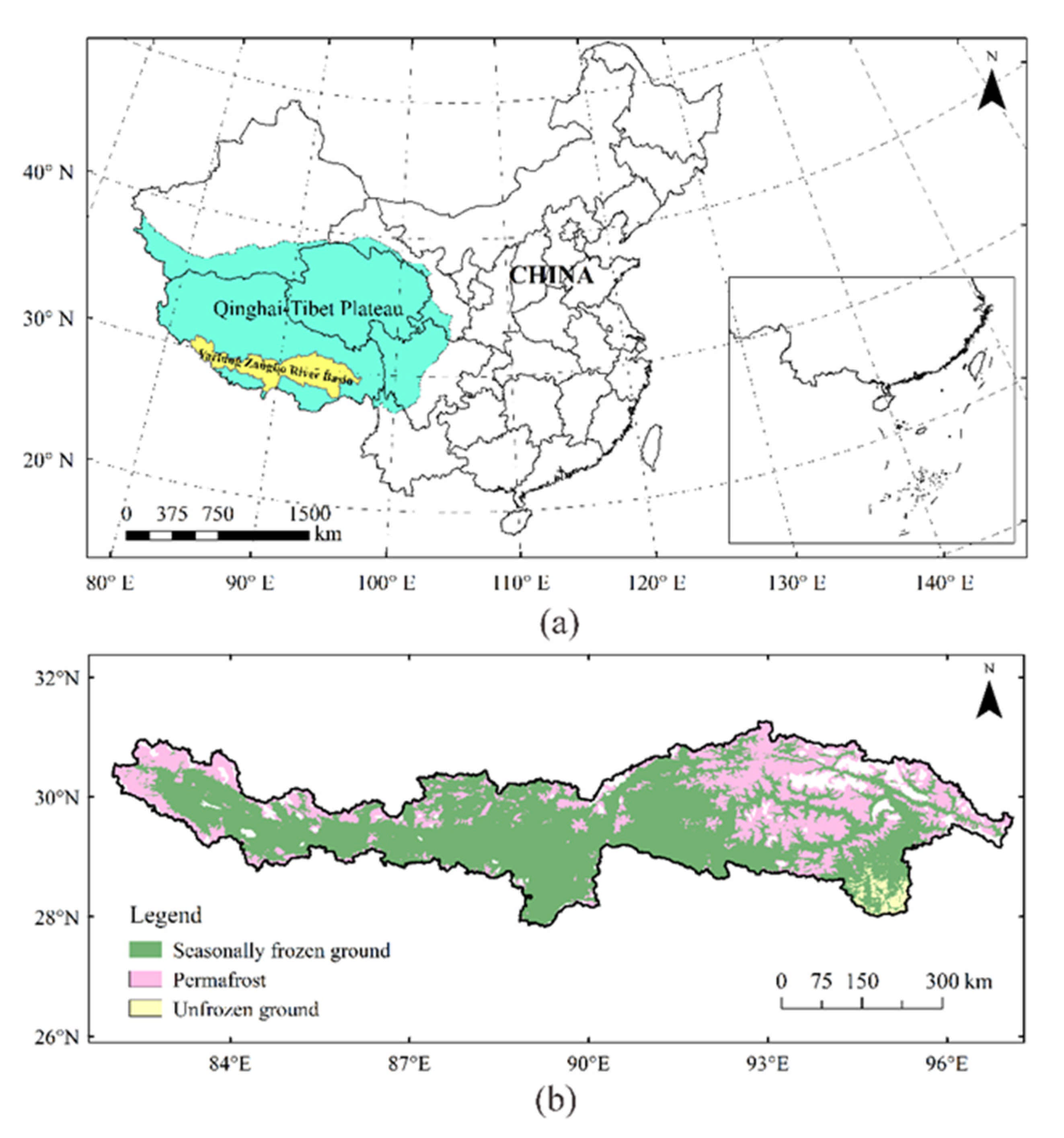
2.1. Study Area

The YZRB is located at 27–32°N and 82–97°E, in the southeast of the QTP and the northern foothills of the Himalayas (Figure 1), with a basin area of about 240,000 km2 and a main stream length of more than 2000 km [29]. The topography of the YZRB is high in the west and low in the east, with large vertical differences in altitude [30]. The YZRB is rich in water resources [31], and the condition of the water resources in the basin is closely related to the water security of Tibet, India, Bangladesh, and other countries in the downstream area. The upstream area of the YZRB has an average altitude of 4600 m above sea level and is mainly distributed with alpine valleys and other landforms [32]; the midstream region is mainly the southern Tibetan valley, which has a warm and semi-arid climate and is an area with a high intensity of human activities [33]; the downstream area includes a highland temperate humid and semi-humid climate zone and a mountainous subtropical humid climate zone with a relatively warm and humid climate [34]. The Yarlung Zangbo River is one of the highest rivers in the world, and due to its special topographic conditions and altitude, the basin presents the characteristics of being sensitive and vulnerable to climate change [35]. Especially in recent decades, the permafrost in the YZRB has been melting, and the active layer has become thicker [36]. At the same time, the glaciers have retreated significantly [37]. All these changes have had a substantial impact on the ecological environment and water resource protection in the basin. Therefore, accurate estimation of TWSC in the YZRB can help enhance the understanding of the mechanisms of hydrology and ecosystem changes in response to human activities as well as climate change at the background of global warming.

2.2. Data

The two datasets used for TWSC estimation in this study are the fifth-generation reanalysis product of the European Centre for Medium-Range Weather Forecasts (ERA5) data and the Global Land Surface Data Assimilation (GLDAS) data. Total precipitation, evapotranspiration, total runoff, soil moisture, and snow water equivalent from these two datasets were used to estimate TWSC, respectively, and the estimated TWSC was then compared with the TWSC derived from GRACE. In addition, before comparisons with GRACE-derived TWSC, the relevant mean of each grid was removed from the TWSC obtained based on ERA5 and GLDAS so that they could be compared with GRACE-derived TWSC.

2.2.1. GRACE Data

The GRACE gravity satellite is a two-satellite system developed by the National Aeronautics and Space Administration (NASA) in cooperation with the German Aerospace Center (DLR) and was successfully launched in March 2002. Since the launch of satellite, the Gravity Recovery and Climate Experiment (GRACE) has provided pioneering observations of global mass flux that have contributed significantly to our understanding of large-scale changes in polar ice, ground water storage, and ocean mass distribution [39,40,41]. In particular, GRACE has been widely used for monitoring terrestrial water storage with excellent performance. Currently, the Center for Space Research (CSR) at the University of Texas, the German Research Centre for Geosciences (GFZ), and the Jet Propulsion Laboratory (JPL) are providing a more mature GRACE product [42]. The GRACE mascon product from JPL RL06M Version 2.0 [43] for the years 2003–2017 (https://grace.jpl.nasa.gov/data/get-data/jpl_global_mascons/ (accessed on 3 May 2020)) with a spatial resolution of 0.5° × 0.5° was used. In this study, the unit of GRACE-derived TWSC is converted to millimeters.

2.2.2. ERA5 Reanalysis Data

The ERA5-Land monthly averaged data used in this study are the latest fifth-generation global atmospheric reanalysis data (ERA5) provided by ECMWF (https://cds.climate.copernicus.eu/cdsapp#!/dataset/reanalysis-era5-land-monthly-means?tab=form (accessed on 11 May 2020)) [44], which have improved spatial resolution to 0.1° × 0.1° compared to the previous version, and their accuracy has also improved compared to ERA-interim.

2.2.3. GLDAS Data

The Global Land Data Assimilation System was jointly developed by the Goddard Space Flight Center (GSFC) of the National Aeronautics and Space Administration (NASA) and the National Environmental Prediction Center (NCEP) of the National Oceanic and Atmospheric Administration (NOAA), which can provide users with multiple data products (https://disc.gsfc.nasa.gov/datasets (accessed on 12 May 2020)) [45]. Currently, the GLDAS provides a large number of land surface data products in combination with four land surface models: Mosaic, NCEP, OSU, Air Force, and Office of Hydrology (NOAH), the Community Land Model (CLM), and the Variable Infiltration Capacity (VIC). These high-quality global land surface data products have been widely used in analysis of TWSC [46], the monitoring of droughts [47], and assessments of climate and hydrological change [48]. Compared to other GLDAS products, the NOAH has a higher spatial resolution and a longer time span. Therefore, the GLDAS_NOAH025_M 2.0 and GLDAS_NOAH025_M 2.1 products (https://disc.gsfc.nasa.gov/datasets?keywords=GLDAS&page=1&temporalResolution=1%20month&spatialResolution=0.25%20%C2%B0%20x%200.25%20%C2%B0 (accessed on 2 July 2020)) were used in this study to estimate the TWSC.

2.3. Methods

The terrestrial water balance method and the summation method were used to estimate the TWSC of the YZRB based on ERA5 and GLDAS, respectively. By generating four sets of TWSC estimation, a quantitative performance evaluation on different datasets and different methods for terrestrial water storage estimation in the YZRB was implemented, by taking the TWSC derived from GRACE as the validation data. Given that the spatial resolution of GRACE-derived TWSC is 0.5° × 0.5°, the TWSC estimated from ERA5 and GLDAS was interpolated to 0.5° × 0.5° based on the bilinear interpolation method to compare it with TWSC derived from GRACE.

2.3.1. The Terrestrial Water Balance Method

The terrestrial water balance method (hereafter called PER) means that, for any given region, the monthly TWSC can be estimated by the following terrestrial water balance equation:
S t t = P t E t R t  
where S(t) is the terrestrial water storage in time t, P(t) (mm) is the total precipitation, E(t) (mm) is the evapotranspiration, and R(t) (mm) is the total runoff (surface runoff and groundwater runoff) in this region [49].

2.3.2. The Summation Method

TWSC can also be expressed in terms of changes in its major constituents, and numerous studies have shown that the TWSC estimated from changes in soil moisture and snow water equivalent is in good agreement with the TWSC inferred from GRACE at both global and basin scales [50,51]. The following equation is an approximation of TWSC by the summation method (hereafter called SS) using changes in soil moisture and snow water equivalent:
S t t =   S o t + S n t t  
where So(t) (mm) and Sn(t) (mm) are the soil moisture and snow water equivalent in a given region and at time t (month), respectively. The reasons for neglecting groundwater and other components are explained in the Appendix A (Figure A1).

2.3.3. Evaluation Metrics

In order to accurately assess the spatial and temporal variability characteristics of TWSC, the following indicators were used in this study. A linear regression model was used to detect temporal variation trends of TWSC and can be expressed as follows [52]:
y = a x + b
where y represents the TWSC, x represents time, a represents the slope, and b represents the intercept. a > 0 indicates an increasing trend of TWSC, while a < 0 indicates a decreasing trend.
The Pearson correlation coefficient was applied to analyze the correlation between different variables:
  R x y = i = 1 n x i x ¯ y i y ¯ i = 1 n x i x ¯ 2 i = 1 n y i y ¯ 2
where x i and y i are two series of paired data, n is the number of data pairs, and x ¯ and y ¯ are the average values of each set of data, respectively. R x y represents the consistency between the two variables, ranging from −1 to 1. R x y > 0 means the two have a positive correlation, R x y < 0 means the two have a negative correlation, and a larger absolute value of R x y means a greater correlation between the two series of paired data [53]. The significance level for the linear trend and correlation coefficient was 0.05 in this study.
Additionally, it is not enough to describe only the characteristics of basin-averaged TWSC, and grid-based calculation has great potential for describing the spatial differences of TWSC [54]. In order to reflect the spatial heterogeneity of TWSC more accurately, the linear trends of TWSC and correlation coefficients during 2003–2017 were further calculated in each grid.
Non-parametric statistics are usually much less affected by the presence of outliers and other forms of non-normality. The Mann–Kendall test is a non-parametric test recommended by the World Meteorological Organization that can objectively reflect the trends of time series and has been widely used in the analysis of climatological and hydrological time series data [55,56]. It is resistant to the influence of extremes and performs well with skewed variables and can handle missing values [57]. For time series data Xt = (x1, x2, …, xn), the statistic Zc is calculated as follows:
Z c = s 1 D s s > 0 0 s = 0 s + 1 D s s < 0
s = i = 1 n 1 j = i + 1 n s g n ( x j x i ) , 1 < i < j < n
β = m e d i a n x j x i j i
where xi and xj are the sequential data values, n is the length of the time series, D(s) represents the variance of s, a positive value of β indicates an “upward trend”, and a negative value of β indicates a “downward trend”. When |Zc| > Z(1−α/2) is satisfied, where α is the significance level, there is a statistically significant trend. In this study, the Mann–Kendall test was used to detect the trend of long-term (1948–2017) variation characteristics of TWSC and its components at a significance level of 0.01.
It has been indicated that wavelet analysis can be used to reveal the break point, change, and distribution of periodic variation in the different time scales of the hydrological time series [58]. Therefore, the Morlet wavelet and the wavelet variance were used to reflect the long-term variation characteristics of TWSC and identify abrupt change in this study. For the wavelet function ψ t L 2 R , the continuous wavelet format is defined as:
ψ a , b t = a 1 / 2 ψ a b a a , b R ,   a 0
For the discrete series x(kΔt), (k = 1, 2, …, N), the wavelet transform coefficient can be expressed as follows:
W f a , b = a 1 / 2 Δ t k = 1 N f k Δ t ψ ¯ k Δ t b a
The wavelet variance Var(a) can be calculated as follows [59]:
V a r a = W f a , b 2 d b  
where a is the scale parameter, b is a parameter for horizontal shift, ψa,b(t) is the mother wavelet, Wf (a, b) is the wavelet transform coefficient, and Δt is the sample time interval.

3. Results

3.1. Performance Evaluation of Different TWSC Estimations

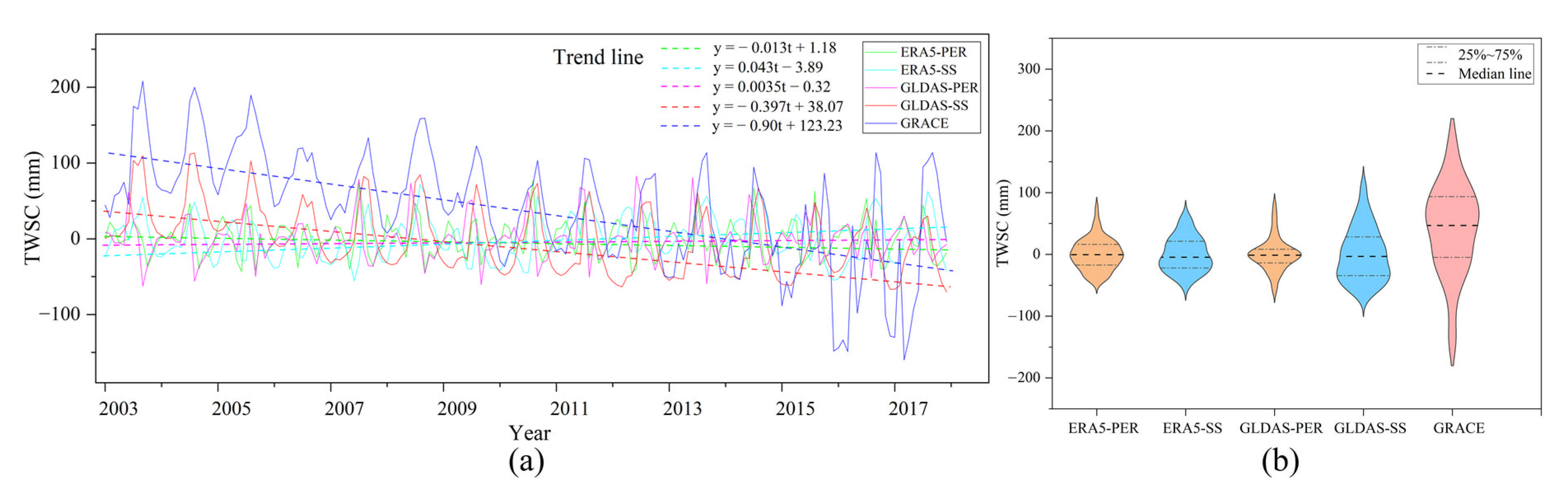
3.1.1. Comparative Analysis of Temporal Characteristics of TWSC

Figure 2 shows the monthly variation trend (a) and changing magnitude (b) of TWSC from 2003 to 2017 estimated by ERA5 and GLDAS with the PER method and the SS method, which were compared with the TWSC derived from GRACE. As shown in Figure 2a, the TWSC of the YZRB derived from GRACE decreased at a rate of 0.9 mm/month during 2003–2017, which is equivalent to 246 million ton/year. The results of ERA5-PER and ERA5-SS decreased at a rate of 0.013 mm/month and increased at a rate of 0.043 mm/month, respectively, while the results of GLDAS-PER and GLDAS-SS increased at a rate of 0.0035 mm/month and decreased at 0.397 mm/month, respectively. It can be seen that there is a large variability in TWSC estimated by different datasets and different methods, among which the trend of GLDAS-SS is most consistent with the results derived from GRACE.
As shown in Figure 2b, the variation amplitudes of ERA5-PER and ERA5-SS are −44.77~77.15 mm and −50.04~71.81 mm, respectively, while those of GLDAS-PER and GLDAS-SS are −62.22~82.97 mm and −69.54~113.36 mm, all of which are somewhat different from the TWSC amplitude from GRACE (−159.23~208.19 mm). The variation amplitude of GLDAS-SS is much closer to that of GRACE compared to the other three sets of TWSC. In addition, we further calculated the correlation coefficients between four sets of TWSC and GRACE-derived TWSC, which are −0.034 (ERA5-PER), 0.36 (ERA5-SS), −0.12 (GLDAS-PER), and 0.75 (GLDAS-SS). It can be seen that the monthly variation of TWSC estimated by the SS method correlates better with GRACE than that of PER. In summary, GLDAS-SS is more consistent with the GRACE-derived TWSC in terms of monthly-scale variation trends and amplitudes.
To further evaluate the performance of TWSC estimations based on ERA5 and GLDAS with PER and SS methods, the multi-year monthly average variation of TWSC from 2003–2017 was compared with the TWSC derived from GRACE. As shown in Figure 3a, GLDAS-SS shows the most similar monthly variation pattern to GRACE in terms of the range of variation and the months in which the peaks and valleys occur. GRACE reaches its maximum and minimum values in September and January with values of 114.09 and −15.81 mm, respectively. GLDAS-SS reaches the maximum and minimum values of 64.01 and −33.50 mm in August and February, respectively. Moreover, GRACE-derived TWSC shows a significant time-lag of about 2 months compared to TWSC estimated by the PER method. As shown in Figure 3b, the correlation coefficients between the two estimations of TWSC based on ERA5 and TWSC derived from GRACE are −0.028 and 0.73, respectively, while the correlation coefficients between the two estimations of TWSC based on GLDAS and TWSC derived from GRACE are −0.16 and 0.95, respectively. Obviously, compared to the PER method, the multi-year monthly average variation of TWSC estimated by the SS method displays a better correlation with that of TWSC derived from GRACE.
With the combination of results indicated by the monthly variation trend and amplitude, GLDAS-SS is most consistent with TWSC derived from GRACE in terms of the temporal characteristics.

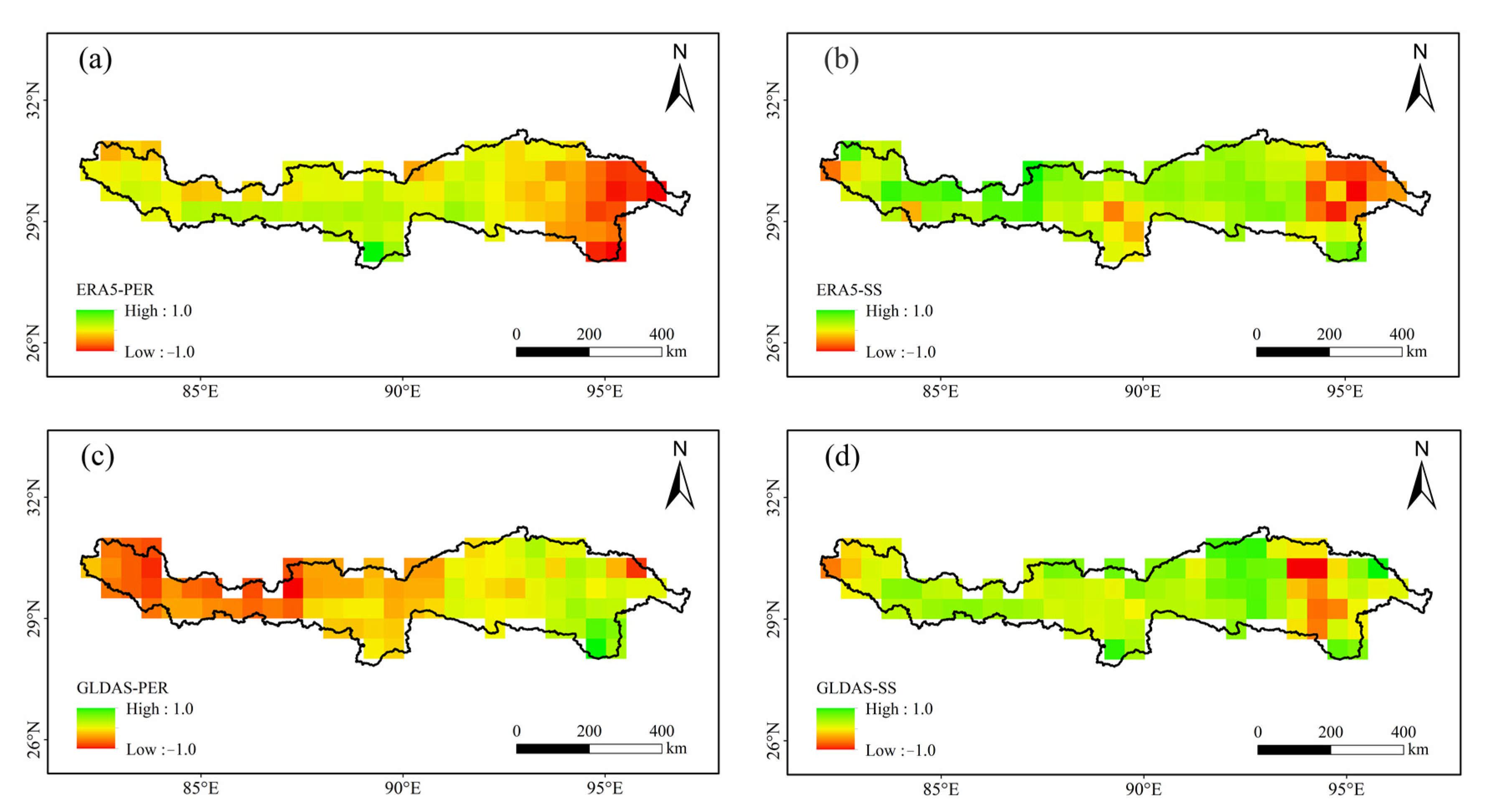
3.1.2. Comparative Analysis on Spatial Characteristics of TWSC

Figure 4 shows the spatial distribution of the correlation coefficients between four TWSC estimations and GRACE-derived TWSC. The correlation coefficients of ERA5-PER and ERA5-SS are lower in the downstream Nyang River basin and higher in the upstream and midstream regions, with maximum values of 0.37 and 0.67, respectively. Different from results obtained by ERA5, the correlation coefficient between GLDAS-PER and GRACE is much lower over the whole basin, especially in the upstream, the lowest value being −0.31, and only slightly high in areas below Nyingchi, with a maximum value of 0.21. Although the TWSC estimation based on GLDAS using the PER method shows poor performance in the YZRB, the correlation coefficient of GLDAS-SS is relatively higher in most parts of the basin, with more than 61.3% of the area higher than 0.5 and a maximum value of 0.82, while the areas with lower correlation coefficients are mainly concentrated in the downstream Nyang River basin. In addition, the TWSC estimated by the SS method performed better than the PER method both based on ERA5 and GLDAS. It is noteworthy that areas with poor correlations are mainly concentrated in the downstream Nyang River basin, where the largest glacier of Parlung Zangbo is distributed [60]. The elevation variation of snowline height in this region exceeds 2000 m [61], which is influenced by the special altitude and topography, causing a large uncertainty of remotely sensed monitoring and data assimilation. Therefore, it is difficult for the TWSC estimated by GLDAS to accurately reflect the terrestrial water storage in this region. Consistent with the results of the comparative analysis on temporal variation characteristics, the TWSC estimated by the SS method based on GLDAS shows the best spatial correlation with the results derived from GRACE.
Performance evaluation of TWSC estimations based on ERA5 and GLDAS with PER and SS methods indicates that TWSC estimated by the SS method is more consistent than the PER method in both temporal and spatial patterns with TWSC derived from GRACE. With regard to the effect of different data sources from ERA5 and GLDAS, TWSC estimated by the SS method based on GLDAS is most consistent with the results from GRACE. Therefore, the SS method based on GLDAS is more suitable for the estimation of TWSC in the YZRB, which provides an important reference for the accurate description of terrestrial water storage change in alpine regions.

3.2. Long-Term Variations of TWSC in the YZRB from 1948 to 2017

3.2.1. Temporal Variation Characteristics

As shown in Figure 5, TWSC in the YZRB showed a significantly increasing trend (p < 0.01) during 1948–2017, but an abrupt change to a decreasing trend occurred in 2002. Specifically, TWSC in the YZRB showed a significantly increasing trend with a rate of 0.0236 mm/month before 2002 (p < 0.01) and a significantly decreasing trend with a rate of 0.397 mm/month after 2002 (p < 0.01). This is consistent with the results of Liu et al. [62] in a study of the dry and wet transition characteristics of the YZRB; the YZRB showed an overall wetting trend from 1982 to 2015, but the basin showed a significant aridity trend after the turn of the 21st century.
To further validate the time when the abrupt change in TWSC occurred, wavelet analysis was adopted to explore the long-term periodic variation of TWSC in the YZRB during 1948–2017. As shown in Figure 6a, there are more complex periodic oscillations in TWSC as the time scale decreases. In terms of large-scale cycles, corresponding to the upper part of the time-frequency distribution chart, there is a large-scale oscillation cycle of TWSC of about 42 years, but given that the total length of the time series is 70 years, a large-scale cycle of about 42 years should not be taken into consideration. As to the mesoscale cycle, corresponding to the middle part of the wavelet coefficient contour plot, a mesoscale oscillation cycle of about 24 years is shown, with about three peaks and valleys. For the small-scale cycle, corresponding to the lower part of the wavelet coefficient contour plot, a small-scale oscillation cycle of about 5 years during 1948–1975 and about 8 years during 1976–2017 is shown. In addition, the wavelet variance map shown in Figure 6b indicates that the dominant cycle of the annual variation of terrestrial water storage during 1948–2017 is 35 years. Nevertheless, TWSC presents opposite values before and after 2002 at different time scales, further demonstrating that TWSC experienced mutation around 2002.

3.2.2. Spatial Variation Characteristics

As shown in Figure 7a, TWSC of the YZRB showed an increasing trend from upstream to downstream during 1948–2017, with a minimum value of 10.26 mm in the western part of the upper YZRB and a maximum value of 38.36 mm in the southeastern part of the downstream. The terrestrial water storage in the middle reaches remained basically unchanged with a slightly increasing tendency. By combining the temporal variation characteristics of TWSC (Figure 6), the significantly increasing trend of TWSC in the YZRB was mainly ascribed to the increase in terrestrial water storage in the middle and lower reaches. A “dry gets wetter, wet gets drier” paradigm was identified, which is in contrast with the widely accepted “dry gets drier, wet gets wetter” paradigm. As shown in Figure 7b, only 18.96% of the total basin area showed an increasing trend, while 81.04% of the basin exhibited a decreasing trend, mainly distributed in wet regions, including the “One River and Two Tributaries” regions (the middle reaches of the Yarlung Zangbo River and its two longest tributaries, the Lhase River and the Nianchu River) and the southeastern downstream regions. In addition, the initial “dry gets drier, wet gets wetter” paradigm has been challenged by many other studies. For example, it has been found that only 10.8% of the global land area shows a robust “dry gets drier, wet gets wetter” pattern, compared to 9.5% of global land area with the opposite pattern, i.e., “dry gets wetter, and wet gets drier” [63]. Consistent with the pattern of “wet gets drier”, increases in aridity are also found in humid tropical Africa, Indonesia, and coastal regions of South America [64].
In order to explicitly explore the spatial variation characteristics of TWSC from 1948 to 2017, the spatial distribution of the multi-year average TWSC and its trend in the YZRB before and after 2002 were further studied. As shown in Figure 8a, the terrestrial water storage in the upstream area of the YZRB decreased during 1948–2002, while the terrestrial water storage in the middle and lower reaches of the YZRB increased; however, Figure 8b illustrates that most of the middle and lower reaches experienced a decreasing trend of TWSC during 1948–2002, indicating a transition from wet to dry in the YZRB, especially in the humid southeastern downstream regions. Due to the continuously decreasing trend of TWSC in the midstream and southeastern downstream regions during 1948–2002, the negative values of TWSC in most areas of the YZRB occurred after 2002 (Figure 8c), causing a more serious threat of drought. Fortunately, the trend of drying was greatly alleviated after 2002. As shown in Figure 8d, TWSC showed an increasing trend in most regions of the YZRB except for the southeastern part of the downstream, which is mainly attributed to the considerable water consumption from the greening of vegetation [65].
It is necessary to emphasize that there is an obvious transition from wet to dry indicated by the changes in terrestrial water storage occurring in the middle reaches from 1948 to 2017. The most obvious land-use changes were observed in the middle reaches of the YZRB, where dense populations and cities led to more human activities [66]. Cuo et al. further revealed that human activities induced 2-fold residential area and 5-fold tree nursery area expansions during 1979–2015 at the expense of cropland, dense forest, and grassland [67], which consumed more water and could result in a serious challenge for water resources in the YZRB. In addition, as the primary type of human activities on the QTP, grazing is believed to have caused severe grassland degradation or even desertification [68], which was responsible for the drying trend in the middle reaches.

4. Discussion

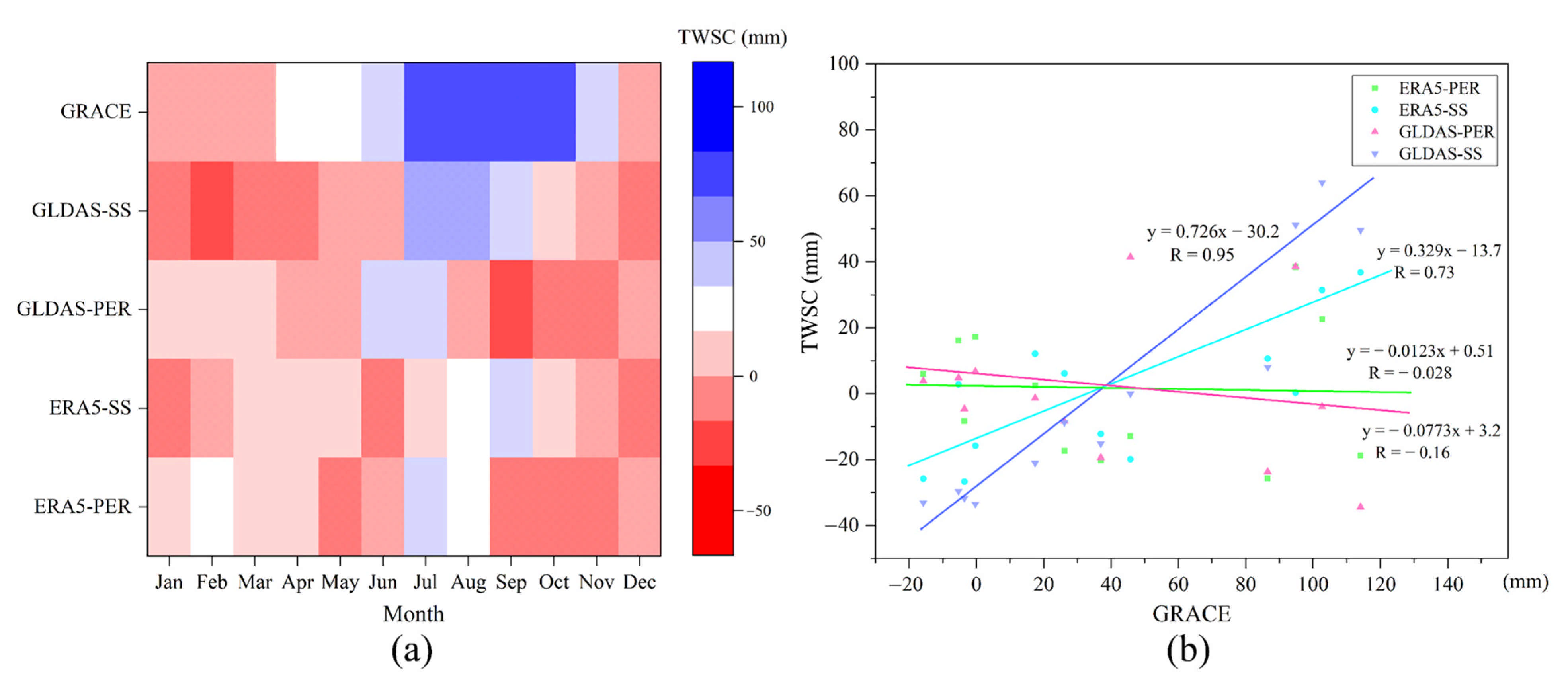
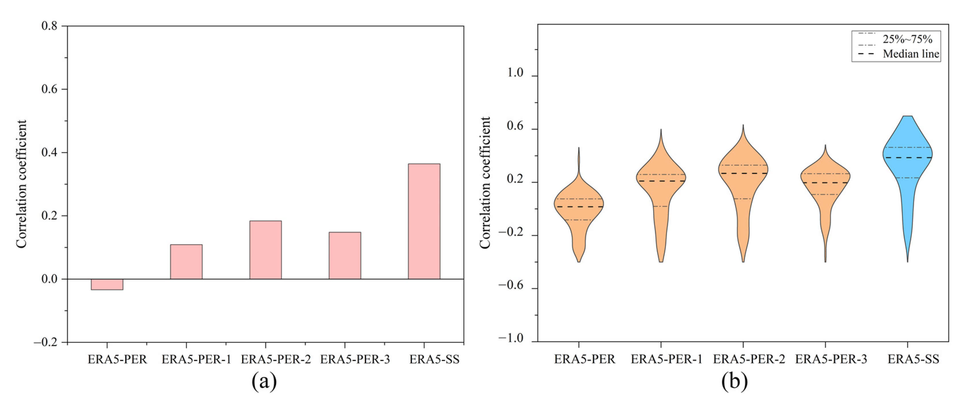
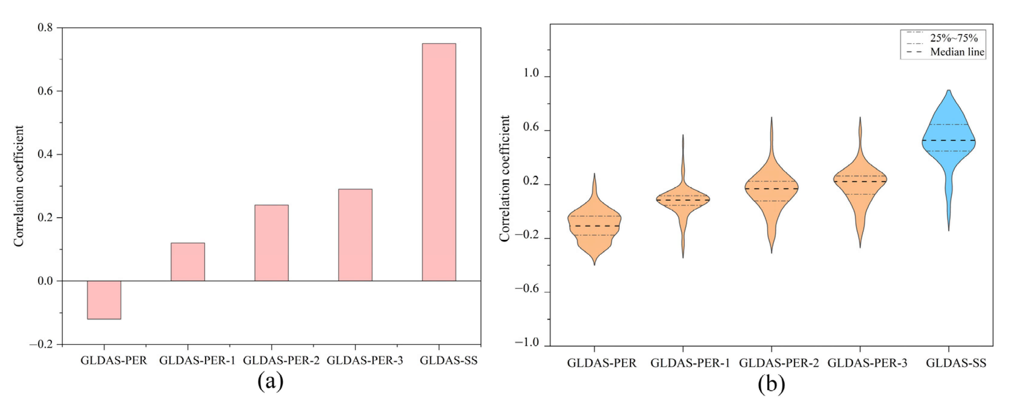
4.1. Time-Lag Effect of Monthly TWSC Estimations

The time-lag effect has been demonstrated in many previous studies on TWSC estimation [69,70] and cannot be neglected when improving the estimation accuracy for TWSC. Similarly, as shown in Figure 3a, GRACE-derived TWSC also showed a significant time-lag correlation with TWSC estimated by the PER method based on ERA5 and GLDAS. Given that TWSC estimated by the SS method performed better than the PER method in both temporal and spatial patterns, the differences in the time-lag correlation between the monthly TWSC estimated by the PER method and GRACE-derived TWSC from 2003 to 2017 were further investigated.
Figure 9 shows the analysis results of the time-lag effect of TWSC estimated by the PER method based on ERA5. Based on the ERA5, the correlation coefficient between the TWSC estimated by the PER method with zero time lag and GRACE-derived TWSC is −0.03, while the correlation coefficients are 0.11, 0.18, and 0.15 with 1-month, 2-month, and 3-month lags, respectively. Apparently, the correlation coefficient of TWSC reaches a maximum value of 0.18 at a time-lag of 2 months, which is still smaller than that of 0.36 estimated by the SS method, indicating that the PER method has limitations in estimating TWSC in the YZRB. As shown in Figure 9b, the amplitude of the correlation coefficient estimated by the PER method based on ERA5 is closest to that estimated by the SS method at a lag of 2 months, which is consistent with the time lag in the study of Zhou et al. [71]. The basin-averaged values of the correlation coefficients are −0.01, 0.14, 0.19, and 0.16 with zero, 1-month, 2-month, and 3-month lags, respectively, with the highest values at 2-month lag, which are all lower than the basin-averaged value of 0.33 for the TWSC estimated by the SS method.
The time-lag effect of monthly TWSC estimated by the PER method could be attributed to the time consumed from precipitation to runoff, soil moisture, and groundwater [72]. For example, infiltration and recharge to groundwater tend to cause a delay in TWSC. In addition, the time-lagged response of TWSC is dependent on prevailing climatic conditions, an abundance of surface water bodies and vegetation density, topographical factors, and many others [73]. It is interesting to note that hydrologic variables always peak earlier than TWSC; for example, monthly TWSC performs a good correlation with precipitation with a time lag of about 2 months [74]. Therefore, it is the time-lag effect of the PER method that leads to the lack of agreement in estimating TWSC.
In a similar way, based on GLDAS, the time-lag effect of TWSC estimated by the PER method was analyzed. As shown in Figure 10a, the correlation coefficient between the TWSC estimated by the PER method with zero lag and the GRACE-derived TWSC is −0.12, while the correlation coefficients are 0.12, 0.24, and 0.29 with 1-month, 2-month, and 3-month lags, respectively. Different from the results based on ERA5, the correlation coefficient reaches a maximum value of 0.29 at the 3-month lag of TWSC, but it is still much lower than that of 0.75 estimated by the SS method. As shown in Figure 10b, the amplitude of the correlation coefficient calculated by the PER method based on GLDAS is closest to that estimated by the SS method based on GLDAS with a time lag of 3 months. The basin-averaged values of the correlation coefficients are −0.10, 0.08, 0.15, and 0.19 with zero, 1-month, 2-month, and 3-month lags, respectively, with a maximum value of 0.19 at the 3-month lag, which is still lower than that estimated by the SS method based on GLDAS with a value of 0.53. In addition, it is crucial to emphasize that the correlation between the TWSC estimated based on GLDAS and the GRACE-derived TWSC performs better than that based on ERA5, according to Figure 9 and Figure 10.
As indicated in Figure 10b and Figure 11b, the amplitude of the time-lagged correlation coefficients calculated at each one based on the grid is obvious, which can further reveal the spatial heterogeneity of TWSC in the YZRB caused by its significant elevation variation. With a wide range of elevations from 147 m to over 7000 m above sea level, TWSC responds differently to hydrological and climatic conditions at various elevations. Considerable investigations have confirmed that elevation-dependent warming results in vegetation, glaciers, and snow cover, presenting distinctive properties at different altitudes [75,76], which in turn leads to a significant impact on the spatial distribution of TWSC. For example, in the YZRB, when the altitude is higher than 3250 m, the NDVI begins to decline gradually, and the NDVI gradually becomes stable as the elevation approaches 6000 m [77]. In addition, the elevation dependence of the warming rate has a significant implication for QTP water resources and environmental changes, since most glaciers and snow surfaces are located 5000 m above sea level [78]. All these findings account for the spatial heterogeneity of TWSC due to its significant elevation variation.

4.2. Possible Dominant Factors of TWSC

The TWSC of GLDAS-SS is most consistent with the GRACE-derived TWSC in the YZRB and indicates a long-term variation of TWSC from 1948 to 2017. In addition, two critical hydrological variables in alpine regions, soil moisture and snow water equivalent, are available through the SS method, which enables a more accurate attribution analysis of TWSC and makes up for the limitations of the short time series and insufficient spatial data in previous studies.
Since TWSC showed an opposite trend before and after 2002, and to investigate possible dominant factors of TWSC, the year of 2002 was taken as the turning point. As shown in Figure 11, the variation patterns of the soil moisture change and the snow water equivalent change around 2002 were consistent with that of TWSC, further implying the important role of glaciers, snow, and permafrost in alpine region water storage [79]. Specifically, the soil moisture showed a significantly increasing trend with a rate of 0.0144 mm/month during 1948–2002 (p < 0.01) and a significantly decreasing trend with a rate of 0.394 mm/month during 2003–2017 (p < 0.01). The snow water equivalent showed a significantly increasing trend with a rate of 0.0092 mm/month during 1948–2002 (p < 0.01) and a significantly decreasing trend with a rate of 0.0024 mm/month during 2003–2017 (p < 0.01). Based on the method developed by Su et al., calculating the contribution of different components to the changes in terrestrial water storage on the QTP [80], the contributions of the changes in soil moisture and snow water equivalent to TWSC before and after 2002 was quantified in this study. During 1948–2002, the contributions of changes in soil moisture and snow water equivalent to TWSC were 61% and 39%, respectively, while a much more significant domination of soil moisture was identified during 2003–2017; that is, the contributions of changes in soil moisture and snow water equivalent to TWSC were 99% and 1%, respectively.
A more significant contribution of soil moisture change to TWSC after 2002 could be attributed to the degradation of permafrost and melting of snow resulting from rapid warming since the beginning of the 21st century. Climate warming has increased the temperature of permafrost over the QTP, leading to the melting of soil ice in the layers overlying the permafrost as well as the thickening of the active layer [81]. The influence of seasonally frozen ground has been more pronounced than that of permafrost [82]. During the warm season, the stored solid water from seasonally frozen ground can be released, but when the cold season comes, water transforms from liquid to solid stored in soil, further resulting in more significant seasonal changes in soil moisture. Additionally, the increase in seasonally frozen ground will enhance infiltration and the groundwater reservoir capability, thus increasing discharge from soil moisture [83], which in turn causes a more remarkable effect on TWSC. Furthermore, it has been confirmed that the effect of elevation-dependent warming is present at relatively low-elevation ranges but absent when the elevation continues to rise [84]. With the melting of snow and ice at lower altitudes, the snowline gradually retreats over the QTP [85]. In addition, there is less impact on the melting of most glaciers and snow located at elevations above 4800 m [86], accounting for the sharp decrease in the contribution of snow water equivalent changes to the TWSC during 2003–2017 in the YZRB.
The spatial analysis of TWSC further confirms the dominant role of soil moisture, especially during 2003–2017. As shown in Figure 12, the spatial distribution of soil moisture is more consistent with that of TWSC. After 2002, the areas where TWSC and soil moisture decreased were gradually expanding from upstream to downstream, with the most obvious changes in the middle reaches. The areas with reduced TWSC and soil moisture increased by 16.21% and 36.71%, respectively, mainly distributed in the “One River and Two Tributaries” area with a high intensity of human activities, which once again confirmed the important impact of human activities on terrestrial water storage. TWSC and soil moisture in most of the midstream remained unchanged during 1948–2002 but decreased during 2003–2017. The areas where soil moisture decreased during 1948–2002 and 2003–2017 were mainly distributed in the upper reaches, and the areas where soil moisture increased were mainly concentrated in the lower reaches. This may be the result of the relatively high density of vegetation cover in the downstream area due to the relatively low elevation and high temperature, which promotes the water-holding capacity of the soil in the downstream area [87]. The areas where the snow water equivalent decrease during 1948–2002 were mainly concentrated in the upper reaches, and most of the middle and lower reaches mainly showed an increasing trend. In addition, increased snow water equivalent mitigated the drying tendency caused by decreased soil moisture in the eastern part of the upstream and Parlung Zangbo region before 2002. The overall spatial distribution of snow water equivalent in most areas of the YZRB during 2003–2017 was similar to that during 1948–2002, except for the downstream Parlung Zangbo glacier region, which showed a significantly decreasing trend. In contrast to the significantly decreasing trend, both soil moisture and TWSC showed an increasing trend in the Parlung Zangbo glacier region during 2003–2017, further implying the dominant role of soil moisture.

5. Conclusions

In this study, monthly data of ERA5 and GLDAS from 2003 to 2017 were used to estimate TWSC in the YZRB, with the PER method and the SS method. Based on the TWSC derived from GRACE, the performance assessment and time-lag effect of different data sources and methods over the YZRB were conducted, and the SS method based on GLDAS was used to further investigate the spatial and temporal characteristics of terrestrial water storage in the YZRB from 1948 to 2017 and its dominant factors. Conclusions are summarized as follows:
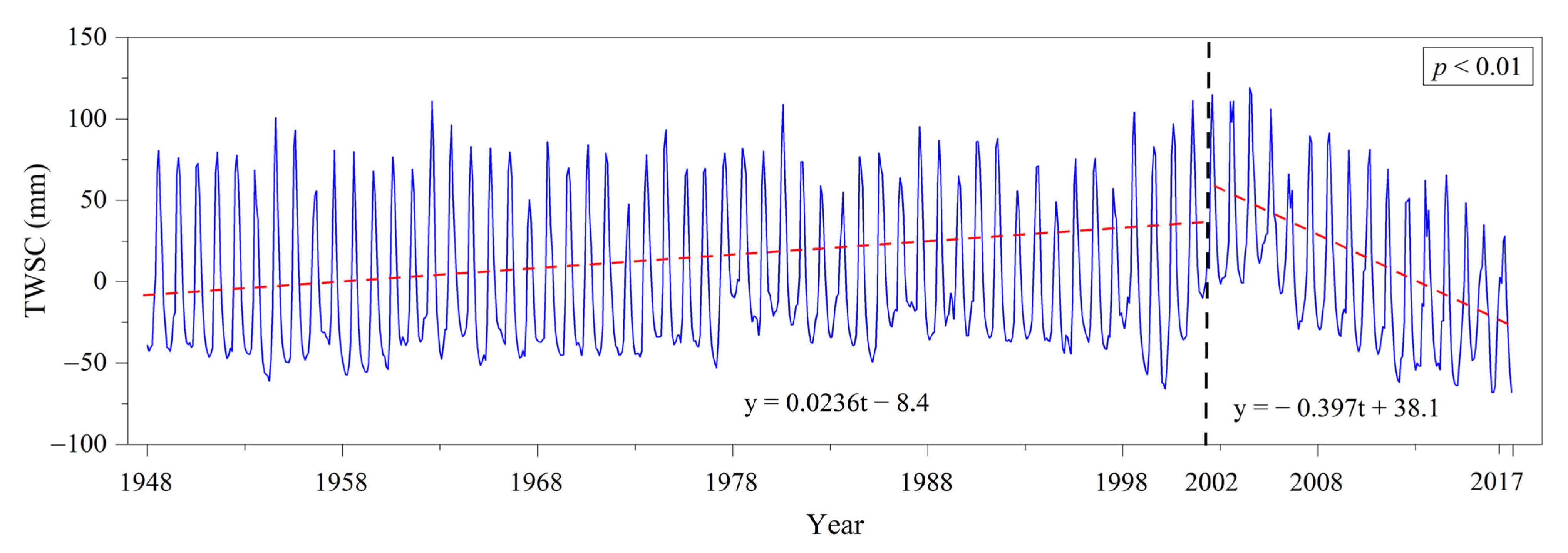
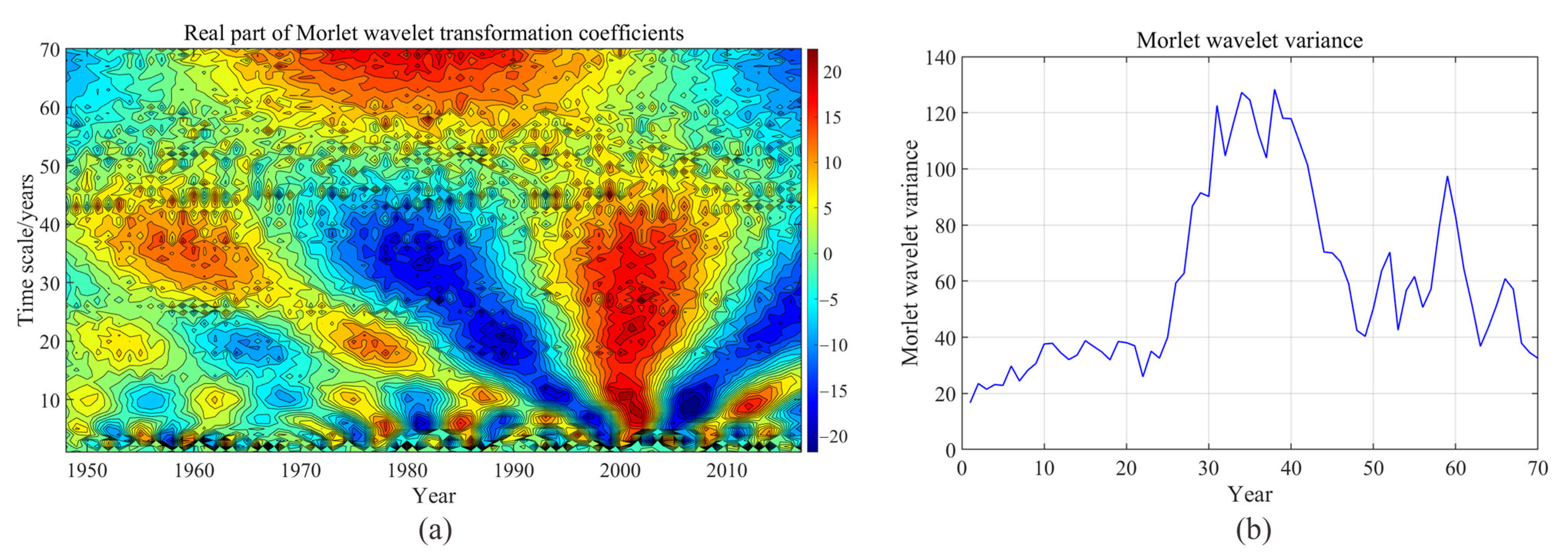
  • The results of the spatial and temporal variations of the four sets of TWSC estimated by combining two datasets and two methods revealed that a 2-month lag and a 3-month time lag exist between the GRACE-derived TWSC and the TWSC estimated by the PER method based on ERA5 and GLDAS, respectively. In addition, the TWSC based on the SS method and GLDAS is most consistent with the results of GRACE, which was further adopted for investigation of the long-term variation characteristics of TWSC in the YZRB by using the Mann–Kendall nonparametric test and wavelet analysis, indicating that an abrupt change in TWSC from increasing to decreasing occurred around 2002, and the dominant cycle of TWSC during 1948–2017 was 35 years.
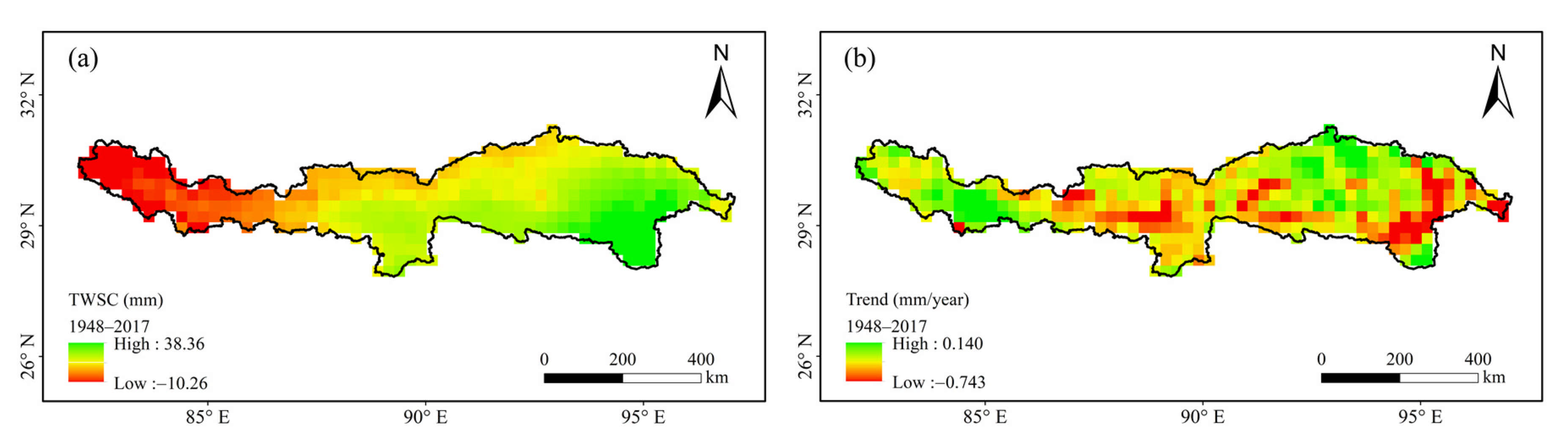
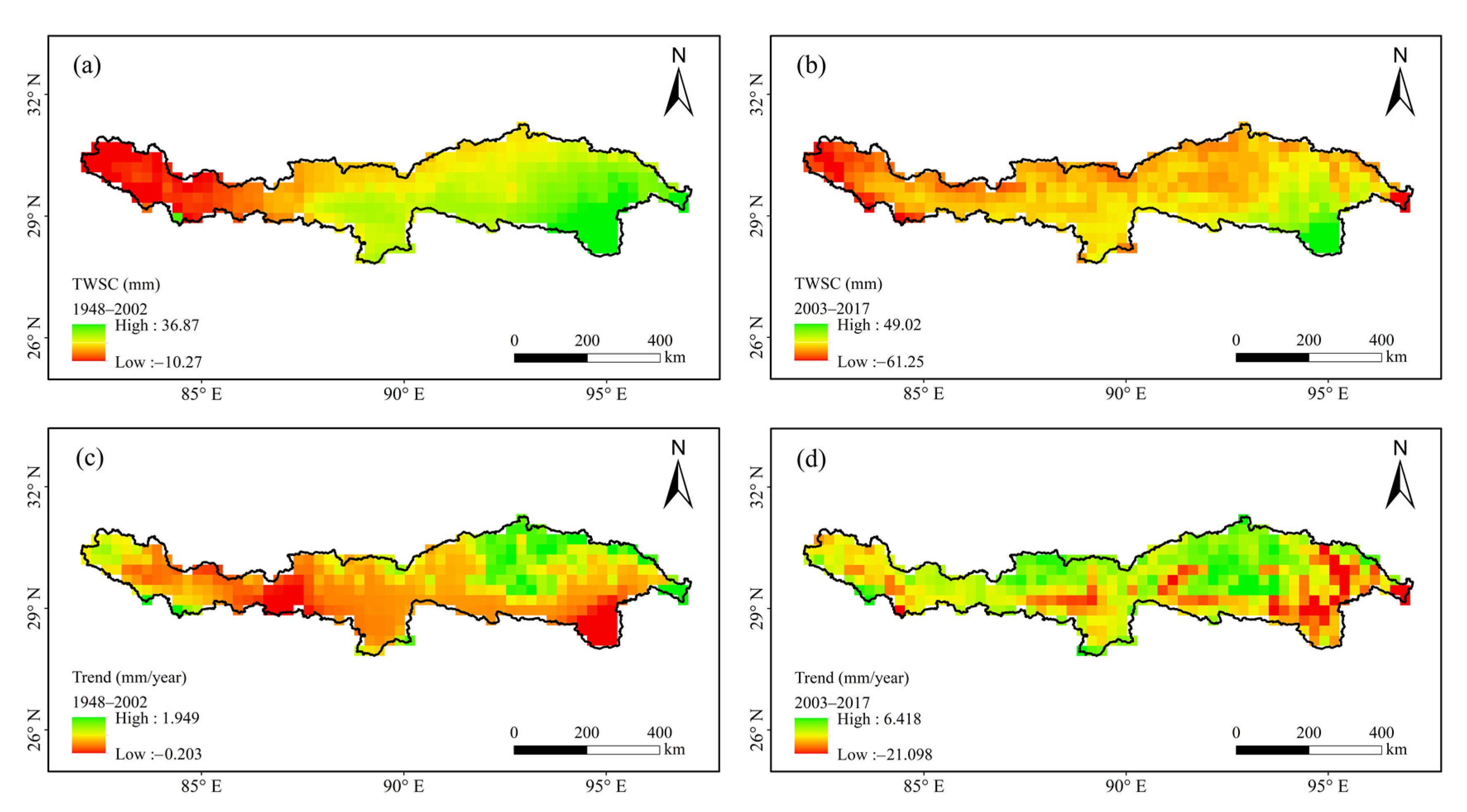
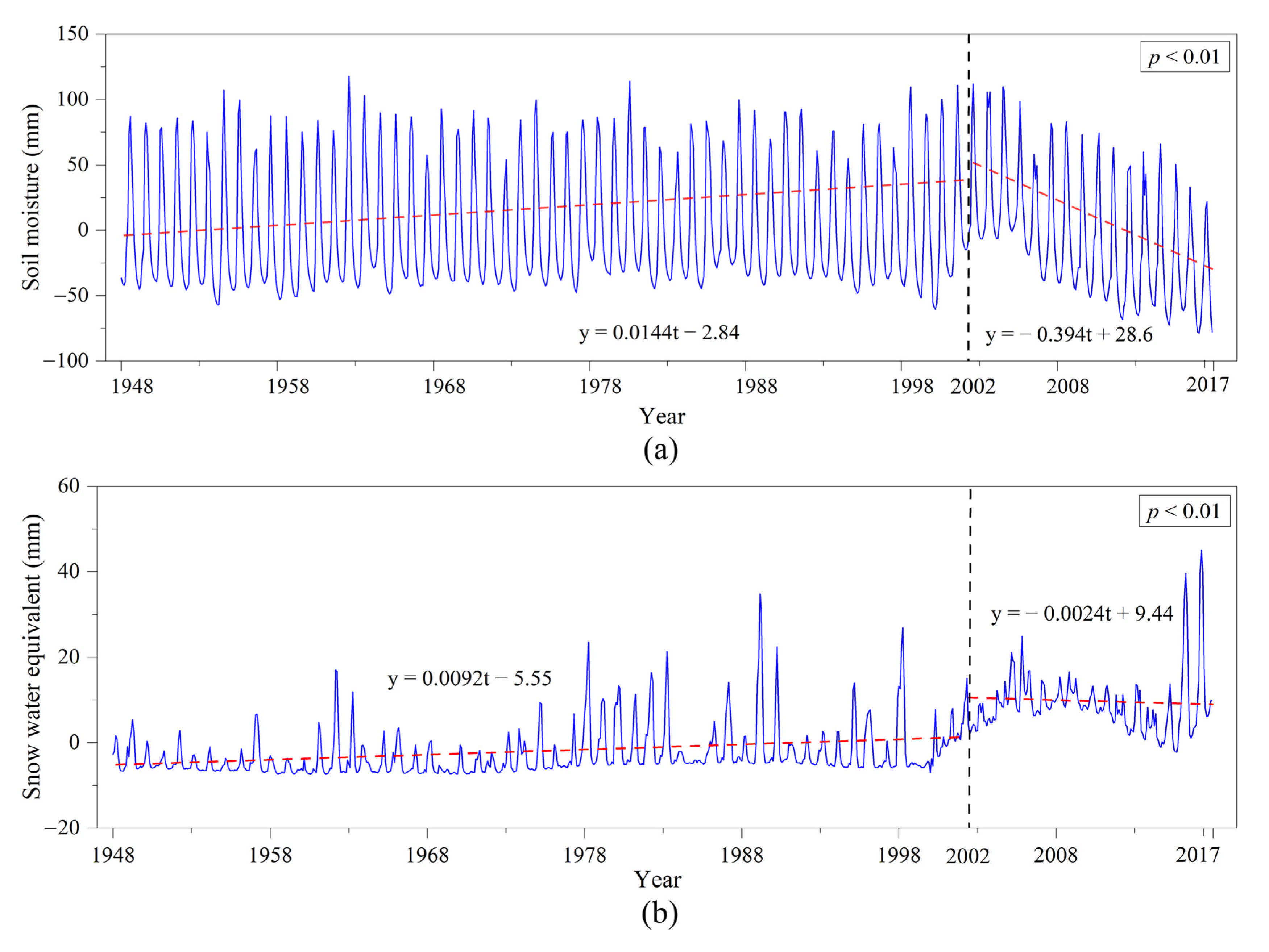
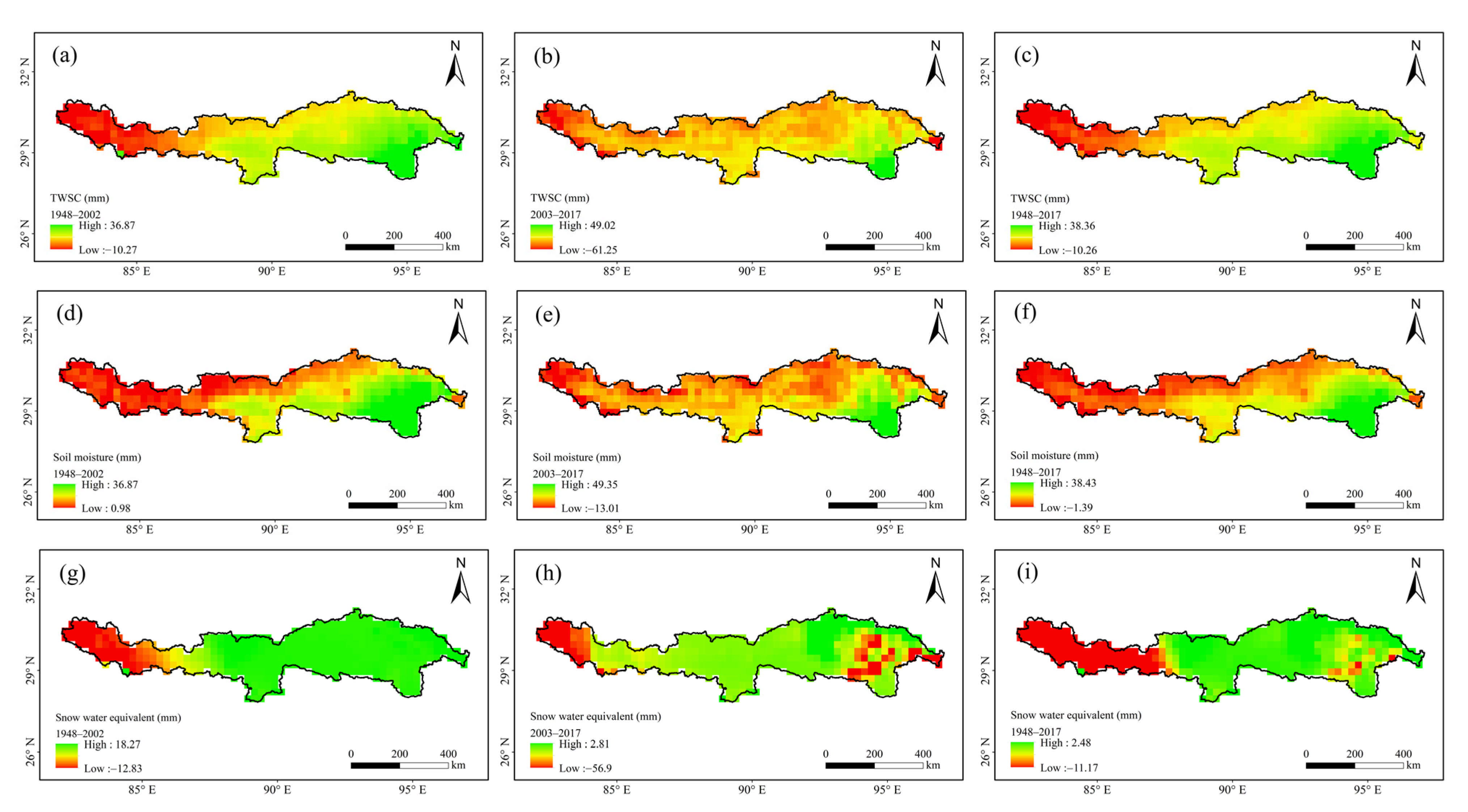
  • During 1948–2017, the change in soil moisture played a dominant role in TWSC over the YZRB, especially after 2002. TWSC, soil moisture, and snow water equivalent changes all showed opposite trends around 2002, i.e., an increasing trend before 2002 and a decreasing trend after 2002. In terms of spatial distribution, TWSC, soil moisture, and snow water equivalent changes all show obvious spatial heterogeneity, mainly reflected in the “One River and Two Tributaries” area, with a high intensity of human activities, and the Parlung Zangbo region, where glaciers are concentrated.
  • The elevation-dependent warming caused by the complex topography of the YZRB not only resulted in the spatial heterogeneity of TWSC, mainly through affecting the distribution of vegetation, glaciers, and snow, but also led to a rapid reduction in the contribution of snow water equivalent change to TWSC after 2002.
Despite the fact that the SS method based on GLDAS data exhibits the best overall agreement with GRACE, groundwater is not taken into account in the SS method. Therefore, the neglect of groundwater information could have contributed to the lack of agreement between the estimates and GRACE. In the future, considering the uneven distributions of groundwater might improve estimation accuracy. The findings in this study can provide an important reference for investigations of the ecohydrological cycle over the YZRB and will be crucial for evaluating the sustainability of water resources of data-scarce alpine regions.

Author Contributions

Conceptualization, L.L.; methodology, L.L. and X.W.; software, X.W.; validation, X.W. and L.L.; formal analysis, L.L. and X.W.; investigation, Q.N. and X.W.; resources, L.L.; data curation, X.W. and H.L.; writing—original draft preparation, L.L and X.W.; writing—review and editing, L.L. and H.L.; visualization, Q.N., X.W. and H.L.; supervision, L.L.; project administration, L.L. and Z.X.; funding acquisition, L.L. and Z.X. All authors have read and agreed to the published version of the manuscript.

Funding

This research was jointly supported by the National Natural Science Foundation of China (51961145104, 52079138, and 91647202), the 2115 Talent Development Program of China Agricultural University (00109019), and National Training Program of Innovation and Entrepreneurship for Undergraduates (2018bj105).

Institutional Review Board Statement

Not applicable.

Informed Consent Statement

Not applicable.

Data Availability Statement

Not applicable.

Acknowledgments

Thanks for GRACE data provided by Jet Propulsion Laboratory, ERA5 reanalysis data provided by the European Centre for Medium Range Weather Forecasts, and GLDAS data provided by the National Aeronautics and Space Administration and National Oceanic and Atmospheric Administration.

Conflicts of Interest

The authors declare no conflict of interest.

Appendix A

Two sensitivity analyses were designed. One (a) is considering changes in groundwater, surface water, and plant canopy interception and the other (b) is only considering change in groundwater. The results of the sensitivity analysis confirm that the performance of (a) and (b) is similar to the results that only soil moisture and snow water equivalent are included by (c), and the basin-averaged values of the correlation coefficient have not been improved as illustrated in (d). The comparison of the results is shown in Figure A1. Furthermore, the changes in snow and permafrost are more obvious in the YZRB, so the changes in snow water equivalent and soil moisture deserve more attention. Therefore, it is reasonable to ignore groundwater and other components.
Figure A1. Results of sensitivity analysis on influencing factors of TWSC based on GLDAS-SS. (a) represents the spatial distribution of correlation coefficient between GLDAS-SS-derived TWSC (taking soil moisture, snow water equivalent, surface water, groundwater, and plant canopy interception into account) and GRACE-derived TWSC; (b) represents the spatial distribution of correlation coefficient between GLDAS-SS-derived TWSC (taking soil moisture, snow water equivalent, and groundwater into account) and GRACE-derived TWSC; (c) represents the spatial distribution of correlation coefficient between GLDAS-SS-derived TWSC (taking soil moisture and snow water equivalent into account as defined in SS method in this study) and GRACE-derived TWSC; (d) illustrates the comparison results among (ac).
Remotesensing 13 02356 g0a1

References

  1. Hirschi, M.; Seneviratne, S.I.; Hagemann, S.; Schär, C. Analysis of seasonal terrestrial water storage variations in regional climate simulations over Europe. J. Geophys. Res. Space Phys. 2007, 112, 112. [Google Scholar] [CrossRef] [Green Version]
  2. Deng, H.; Chen, Y. Influences of recent climate change and human activities on water storage variations in Central Asia. J. Hydrol. 2017, 544, 46–57. [Google Scholar] [CrossRef]
  3. Yeh, P.J.-F.; Famiglietti, J. Regional terrestrial water storage change and evapotranspiration from terrestrial and atmospheric water balance computations. J. Geophys. Res. Space Phys. 2008, 113, 113. [Google Scholar] [CrossRef]
  4. Deng, H.; Chen, Y.; Li, Q.; Lin, G. Loss of terrestrial water storage in the Tianshan mountains from 2003 to 2015. Int. J. Remote. Sens. 2019, 40, 8342–8358. [Google Scholar] [CrossRef]
  5. Xu, M.; Ye, B.; Zhao, Q.; Zhang, S.; Wang, J. Estimation of water balance in the source region of the Yellow River based on GRACE satellite data. J. Arid. Land 2013, 5, 384–395. [Google Scholar] [CrossRef]
  6. Xiang, L.; Wang, H.; Steffen, H.; Wu, P.; Jia, L.; Jiang, L.; Shen, Q. Groundwater storage changes in the Tibetan Plateau and adjacent areas revealed from GRACE satellite gravity data. Earth Planet. Sci. Lett. 2016, 449, 228–239. [Google Scholar] [CrossRef] [Green Version]
  7. Massoud, E.; Liu, Z.; Shaban, A.; Hage, M. Groundwater Depletion Signals in the Beqaa Plain, Lebanon: Evidence from GRACE and Sentinel-1 Data. Remote. Sens. 2021, 13, 915. [Google Scholar] [CrossRef]
  8. Massoud, E.C.; Purdy, A.J.; Miro, M.E.; Famiglietti, J. Projecting groundwater storage changes in California’s Central Valley. Sci. Rep. 2018, 8, 1–9. [Google Scholar] [CrossRef]
  9. Sinha, D.; Syed, T.H.; Famiglietti, J.; Reager, J.T.; Thomas, R.C. Characterizing Drought in India Using GRACE Observations of Terrestrial Water Storage Deficit. J. Hydrometeorol. 2017, 18, 381–396. [Google Scholar] [CrossRef]
  10. Massoud, E.; Turmon, M.; Reager, J.; Hobbs, J.; Liu, Z.; David, C.H. Cascading Dynamics of the Hydrologic Cycle in California Explored through Observations and Model Simulations. Geoscience 2020, 10, 71. [Google Scholar] [CrossRef] [Green Version]
  11. Zhang, G.; Yao, T.; Xie, H.; Yang, K.; Zhu, L.; Shum, C.; Bolch, T.; Yi, S.; Allen, S.; Jiang, L.; et al. Response of Tibetan Plateau lakes to climate change: Trends, patterns, and mechanisms. Earth-Sci. Rev. 2020, 208, 103269. [Google Scholar] [CrossRef]
  12. Chen, H.; Yang, G.; Peng, C.; Zhang, Y.; Zhu, D.; Zhu, Q.; Hu, J.; Wang, M.; Zhan, W.; Zhu, E.; et al. The carbon stock of alpine peatlands on the Qinghai–Tibetan Plateau during the Holocene and their future fate. Quat. Sci. Rev. 2014, 95, 151–158. [Google Scholar] [CrossRef]
  13. Zhang, G.; Yao, T.; Xie, H.; Kang, S.; Lei, Y. Increased mass over the Tibetan Plateau: From lakes or glaciers? Geophys. Res. Lett. 2013, 40, 2125–2130. [Google Scholar] [CrossRef]
  14. Cheng, G.; Jin, H. Permafrost and groundwater on the Qinghai-Tibet Plateau and in northeast China. Hydrogeol. J. 2012, 21, 5–23. [Google Scholar] [CrossRef]
  15. Immerzeel, W.W.; Van Beek, L.P.H.; Bierkens, M.F.P. Climate change will affect the Asian Water Towers. Science 2010, 328, 1382–1385. [Google Scholar] [CrossRef]
  16. Yao, T. Tackling on environmental changes in Tibetan Plateau with focus on water, ecosystem and adaptation. Sci. Bull. 2019, 64, 417. [Google Scholar] [CrossRef] [Green Version]
  17. Yang, M.; Wang, X.; Pang, G.; Wan, G.; Liu, Z. The Tibetan Plateau cryosphere: Observations and model simulations for current status and recent changes. Earth-Sci. Rev. 2019, 190, 353–369. [Google Scholar] [CrossRef]
  18. Zhu, L.; Xie, M.; Wu, Y. Quantitative analysis of lake area variations and the influence factors from 1971 to 2004 in the Nam Co basin of the Tibetan Plateau. Chin. Sci. Bull. 2010, 55, 1294–1303. [Google Scholar] [CrossRef]
  19. Yao, T.; Thompson, L.; Yang, W.; Yu, W.; Gao, Y.; Guo, X.; Yang, X.; Duan, K.; Zhao, H.; Xu, B.; et al. Different glacier status with atmospheric circulations in Tibetan Plateau and surroundings. Nat. Clim. Chang. 2012, 2, 663–667. [Google Scholar] [CrossRef]
  20. Zhang, G.; Yao, T.; Xie, H.; Zhang, K.; Zhu, F. Lakes’ state and abundance across the Tibetan Plateau. Chin. Sci. Bull. 2014, 59, 3010–3021. [Google Scholar] [CrossRef]
  21. Syed, T.H.; Famiglietti, J.; Rodell, M.; Chen, J.; Wilson, C.R. Analysis of terrestrial water storage changes from GRACE and GLDAS. Water Resour. Res. 2008, 44, 44. [Google Scholar] [CrossRef]
  22. Lei, Y.; Yao, T.; Yang, K.; Sheng, Y.; Kleinherenbrink, M.; Yi, S.; Bird, B.W.; Zhang, X.; Zhu, L.; Zhang, G. Lake seasonality across the Tibetan Plateau and their varying relationship with regional mass changes and local hydrology. Geophys. Res. Lett. 2017, 44, 892–900. [Google Scholar] [CrossRef] [Green Version]
  23. Tapley, B.D.; Watkins, M.M.; Flechtner, F.; Reigber, C.; Bettadpur, S.; Rodell, M.; Sasgen, I.; Famiglietti, J.S.; Landerer, F.W.; Chambers, D.P.; et al. Contributions of GRACE to understanding climate change. Nat. Clim. Chang. 2019, 9, 358–369. [Google Scholar] [CrossRef] [PubMed]
  24. Guo, J.; Mu, D.; Liu, X.; Yan, H.; Sun, Z. Water Storage Changes over the Tibetan Plateau Revealed by GRACE Mission. Acta Geophys. 2016, 64, 463–476. [Google Scholar] [CrossRef] [Green Version]
  25. Wang, J.; Chen, X.; Hu, Q.; Liu, J. Responses of terrestrial water storage to climate variation in the Tibetan Plateau. J. Hydrol. 2020, 584, 124652. [Google Scholar] [CrossRef]
  26. Deng, H.; Pepin, N.C.; Liu, Q.; Chen, Y. Understanding the spatial differences in terrestrial water storage variations in the Tibetan Plateau from 2002 to 2016. Clim. Chang. 2018, 151, 379–393. [Google Scholar] [CrossRef] [Green Version]
  27. Moiwo, J.P.; Yang, Y.; Tao, F.; Lu, W.; Han, S. Water storage change in the Himalayas from the Gravity Recovery and Climate Experiment (GRACE) and an empirical climate model. Water Resour. Res. 2011, 47, 47. [Google Scholar] [CrossRef] [Green Version]
  28. Xu, Z.; Cheng, L.; Luo, P.; Liu, P.; Zhang, L.; Li, F.; Liu, L.; Wang, J. A Climatic Perspective on the Impacts of Global Warming on Water Cycle of Cold Mountainous Catchments in the Tibetan Plateau: A Case Study in Yarlung Zangbo River Basin. Water 2020, 12, 2338. [Google Scholar] [CrossRef]
  29. Sun, W.; Wang, Y.; Fu, Y.H.; Xue, B.; Wang, G.; Yu, J.; Zuo, D.; Xu, Z. Spatial heterogeneity of changes in vegetation growth and their driving forces based on satellite observations of the Yarlung Zangbo River Basin in the Tibetan Plateau. J. Hydrol. 2019, 574, 324–332. [Google Scholar] [CrossRef]
  30. Li, X.; Liu, L.; Li, H.; Wang, S.; Heng, J. Spatiotemporal soil moisture variations associated with hydro-meteorological factors over the Yarlung Zangbo River basin in Southeast Tibetan Plateau. Int. J. Clim. 2020, 40, 188–206. [Google Scholar] [CrossRef]
  31. Shen, M.; Wang, S.; Li, Y.; Tang, M.; Ma, Y. Pattern of Turbidity Change in the Middle Reaches of the Yarlung Zangbo River, Southern Tibetan Plateau, from 2007 to 2017. Remote Sens. 2021, 13, 182. [Google Scholar] [CrossRef]
  32. Shen, W.; Li, H.; Sun, M.; Jiang, J. Dynamics of aeolian sandy land in the Yarlung Zangbo River basin of Tibet, China from 1975 to 2008. Glob. Planet. Chang. 2012, 86-87, 37–44. [Google Scholar] [CrossRef]
  33. Li, H.; Li, Y.; Gao, Y.; Zou, C.; Yan, S.; Gao, J. Human Impact on Vegetation Dynamics around Lhasa, Southern Tibetan Plateau, China. Sustainability 2016, 8, 1146. [Google Scholar] [CrossRef] [Green Version]
  34. Li, H.; Shen, W.; Zou, C.; Jiang, J.; Fu, L.; She, G. Spatio-temporal variability of soil moisture and its effect on vegetation in a desertified aeolian riparian ecotone on the Tibetan Plateau, China. J. Hydrol. 2013, 479, 215–225. [Google Scholar] [CrossRef]
  35. Wang, X.; Zhong, X.; Liu, S.; Liu, J.; Wang, Z.; Li, M. Regional assessment of environmental vulnerability in the Tibetan Plateau: Development and application of a new method. J. Arid. Environ. 2008, 72, 1929–1939. [Google Scholar] [CrossRef]
  36. Cheng, G.; Zhao, L.; Li, R.; Wu, X.; Sheng, Y.; Hu, G.; Zou, D.; Jin, H.; Li, X.; Wu, Q. Characteristic, changes and impacts of permafrost on Qinghai-Tibet Plateau. Chin. Sci. Bull. 2019, 64, 2783–2795. [Google Scholar] [CrossRef] [Green Version]
  37. Matsuo, K.; Heki, K. Time-variable ice loss in Asian high mountains from satellite gravimetry. Earth Planet. Sci. Lett. 2010, 290, 30–36. [Google Scholar] [CrossRef]
  38. Zou, D.; Zhao, L.; Sheng, Y.; Chen, J.; Hu, G.; Wu, T.; Wu, J.; Xie, C.; Wu, X.; Pang, Q.; et al. A new map of permafrost distribution on the Tibetan Plateau. Cryosphere 2017, 11, 2527–2542. [Google Scholar] [CrossRef] [Green Version]
  39. Chambers, D.P. Observing seasonal steric sea level variations with GRACE and satellite altimetry. J. Geophys. Res. Space Phys. 2006, 111, 111. [Google Scholar] [CrossRef]
  40. Velicogna, I. Increasing rates of ice mass loss from the Greenland and Antarctic ice sheets revealed by GRACE. Geophys. Res. Lett. 2009, 36, 36. [Google Scholar] [CrossRef] [Green Version]
  41. Luthcke, S.B.; Sabaka, T.; Loomis, B.; Arendt, A.; McCarthy, J.; Camp, J. Antarctica, Greenland and Gulf of Alaska land-ice evolution from an iterated GRACE global mascon solution. J. Glaciol. 2013, 59, 613–631. [Google Scholar] [CrossRef]
  42. Watkins, M.M.; Wiese, D.N.; Yuan, D.-N.; Boening, C.; Landerer, F.W. Improved methods for observing Earth’s time variable mass distribution with GRACE using spherical cap mascons. J. Geophys. Res. Solid Earth 2015, 120, 2648–2671. [Google Scholar] [CrossRef]
  43. Wiese, D.N.; Yuan, D.-N.; Boening, C.; Landerer, F.W.; Watkins, M.M. JPL GRACE Mascon Ocean, Ice, and Hydrology Equivalent Water Height Release 06 Coastal Resolution Improvement (CRI) Filtered Version 1.0. Ver. 1.0. PO.DAAC, CA, USA. 2018. Available online: http://0-dx-doi-org.brum.beds.ac.uk/10.5067/TEMSC-3MJC6 (accessed on 1 June 2020).
  44. Hersbach, H.; Bell, B.; Berrisford, P.; Hirahara, S.; Horányi, A.; Muñoz-Sabater, J.; Nicolas, J.; Peubey, C.; Radu, R.; Schepers, D.; et al. The ERA5 global reanalysis. Q. J. R. Meteorol. Soc. 2020, 146, 1999–2049. [Google Scholar] [CrossRef]
  45. Rodell, M.; Houser, P.; Jambor, U.; Gottschalck, J.; Mitchell, K.; Meng, C.-J.; Arsenault, K.; Cosgrove, B.; Radakovich, J.; Bosilovich, M.; et al. The Global Land Data Assimilation System. Bull. Am. Meteorol. Soc. 2004, 85, 381–394. [Google Scholar] [CrossRef] [Green Version]
  46. Jiang, Z.; Hsu, Y.-J.; Yuan, L.; Huang, D. Monitoring time-varying terrestrial water storage changes using daily GNSS measurements in Yunnan, southwest China. Remote Sens. Environ. 2021, 254, 112249. [Google Scholar] [CrossRef]
  47. Han, Z.; Huang, Q.; Huang, S.; Leng, G.; Bai, Q.; Liang, H.; Wang, L.; Zhao, J.; Fang, W. Spatial-temporal dynamics of agricultural drought in the Loess Plateau under a changing environment: Characteristics and potential influencing factors. Agric. Water Manag. 2021, 244, 106540. [Google Scholar] [CrossRef]
  48. Moghim, S. Impact of climate variation on hydrometeorology in Iran. Glob. Planet. Chang. 2018, 170, 93–105. [Google Scholar] [CrossRef]
  49. Güntner, A.; Stuck, J.; Werth, S.; Döll, P.; Verzano, K.; Merz, B. A global analysis of temporal and spatial variations in continental water storage. Water Resour. Res. 2007, 43, 5416. [Google Scholar] [CrossRef]
  50. Rodell, M.; Famiglietti, J.; Chen, J.; Seneviratne, S.I.; Viterbo, P.; Holl, S.; Wilson, C.R. Basin scale estimates of evapotranspiration using GRACE and other observations. Geophys. Res. Lett. 2004, 31, 31. [Google Scholar] [CrossRef] [Green Version]
  51. Deng, S.; Liu, S.; Mo, X. Assessment of Three Common Methods for Estimating Terrestrial Water Storage Change with Three Reanalysis Datasets. J. Clim. 2020, 33, 511–525. [Google Scholar] [CrossRef]
  52. Li, H.; Liu, L.; Shan, B.; Xu, Z.; Niu, Q.; Cheng, L.; Liu, X.; Xu, Z. Spatiotemporal Variation of Drought and Associated Multi-Scale Response to Climate Change over the Yarlung Zangbo River Basin of Qinghai–Tibet Plateau, China. Remote Sens. 2019, 11, 1596. [Google Scholar] [CrossRef] [Green Version]
  53. Li, H.; Liu, L.; Xu, Z. Greening Implication Inferred from Vegetation Dynamics Interacted with Climate Change and Human Activities over the Southeast Qinghai–Tibet Plateau. Remote Sens. 2019, 11, 2421. [Google Scholar] [CrossRef] [Green Version]
  54. Zhang, Y.; Pan, M.; Wood, E.F. On Creating Global Gridded Terrestrial Water Budget Estimates from Satellite Remote Sensing. Surv. Geophys. 2016, 37, 249–268. [Google Scholar] [CrossRef]
  55. Sharma, S.; Saha, A.K. Statistical analysis of rainfall trends over Damodar River basin, India. Arab. J. Geosci. 2017, 10, 319. [Google Scholar] [CrossRef]
  56. Gocic, M.; Trajkovic, S. Analysis of changes in meteorological variables using Mann-Kendall and Sen’s slope estimator statistical tests in Serbia. Glob. Planet. Chang. 2013, 100, 172–182. [Google Scholar] [CrossRef]
  57. Mishra, A.K.; Özger, M.; Singh, V.P. Trend and persistence of precipitation under climate change scenarios for Kansabati basin, India. Hydrol. Process. 2009, 23, 2345–2357. [Google Scholar] [CrossRef]
  58. Liu, D.; Liu, X.; Li, B.; Zhao, S.; Li, X. Multiple time scale analysis of river runoff using wavelet transform for Dagujia River Basin, Yantai, China. Chin. Geogr. Sci. 2009, 19, 158–167. [Google Scholar] [CrossRef] [Green Version]
  59. Li, R.; Huang, H.; Yu, G.; Yu, H.; Bridhikitti, A.; Su, T. Trends of Runoff Variation and Effects of Main Causal Factors in Mun River, Thailand During 1980–2018. Water 2020, 12, 831. [Google Scholar] [CrossRef] [Green Version]
  60. Chen, R.; Zhou, S.; Li, Y.; Deng, Y. Glacial geomorphology of the Parlung Zangbo Valley, southeastern Tibetan Plateau. J. Maps 2015, 12, 716–724. [Google Scholar] [CrossRef]
  61. Yao, T.; Li, Z.; Yang, W.; Guo, X.; Zhu, L.; Kang, S.; Wu, Y.; Yu, W. Glacial distribution and mass balance in the Yarlung Zangbo River and its influence on lakes. Chin. Sci. Bull. 2010, 55, 2072–2078. [Google Scholar] [CrossRef]
  62. Liu, L.; Niu, Q.; Heng, J.; Li, H.; Xu, Z. Transition Characteristics of the Dry-Wet Regime and Vegetation Dynamic Responses over the Yarlung Zangbo River Basin, Southeast Qinghai-Tibet Plateau. Remote Sens. 2019, 11, 1254. [Google Scholar] [CrossRef] [Green Version]
  63. Greve, P.; Orlowsky, B.; Mueller, B.; Sheffield, J.; Reichstein, M.; Seneviratne, S.I. Global assessment of trends in wetting and drying over land. Nat. Geosci. 2014, 7, 716–721. [Google Scholar] [CrossRef]
  64. Greve, P.; Seneviratne, S.I. Assessment of future changes in water availability and aridity. Geophys. Res. Lett. 2015, 42, 5493–5499. [Google Scholar] [CrossRef] [Green Version]
  65. Li, H.; Jiang, J.; Chen, B.; Li, Y.; Xu, Y.; Shen, W. Pattern of NDVI-based vegetation greening along an altitudinal gradient in the eastern Himalayas and its response to global warming. Environ. Monit. Assess. 2016, 188, 1–10. [Google Scholar] [CrossRef]
  66. Liu, Z.; Yao, Z.; Huang, H.; Wu, S.; Liu, G. LAND USE AND CLIMATE CHANGES AND THEIR IMPACTS ON RUNOFF IN THE YARLUNG ZANGBO RIVER BASIN, CHINA. Land Degrad. Dev. 2012, 25, 203–215. [Google Scholar] [CrossRef]
  67. Cuo, L.; Li, N.; Liu, Z.; Ding, J.; Liang, L.; Zhang, Y.; Gong, T. Warming and human activities induced changes in the Yarlung Tsangpo basin of the Tibetan plateau and their influences on streamflow. J. Hydrol. Reg. Stud. 2019, 25, 100625. [Google Scholar] [CrossRef]
  68. Wang, S.; Duan, J.; Xu, G.; Wang, Y.; Zhang, Z.; Rui, Y.; Luo, C.; Xu, B.; Zhu, X.; Chang, X.; et al. Effects of warming and grazing on soil N availability, species composition, and ANPP in an alpine meadow. Ecology 2012, 93, 2365–2376. [Google Scholar] [CrossRef]
  69. Huang, Q.; Zhang, Q.; Xu, C.-Y.; Li, Q.; Sun, P. Terrestrial Water Storage in China: Spatiotemporal Pattern and Driving Factors. Sustainability 2019, 11, 6646. [Google Scholar] [CrossRef] [Green Version]
  70. Perez, A.M.C.; Blanco, A.C. Combination of MODIS Vegetation Indices, GRACE Terrestrial Water Storage Changes, and In-Situ Measurements for Drought Assessment in Cagayan River Basin, Philippines. J. Nat. Resour. Dev. 2017, 45–55. [Google Scholar] [CrossRef]
  71. Zhou, Y.; Jin, S.; Tenzer, R.; Feng, J. Water storage variations in the Poyang Lake Basin estimated from GRACE and satellite altimetry. Geodesy Geodyn. 2016, 7, 108–116. [Google Scholar] [CrossRef] [Green Version]
  72. Awange, J.; Gebremichael, M.; Forootan, E.; Wakbulcho, G.; Anyah, R.; Ferreira, V.; Alemayehu, T. Characterization of Ethiopian mega hydrogeological regimes using GRACE, TRMM and GLDAS datasets. Adv. Water Resour. 2014, 74, 64–78. [Google Scholar] [CrossRef] [Green Version]
  73. Moghim, S. Assessment of Water Storage Changes Using GRACE and GLDAS. Water Resour. Manag. 2020, 34, 685–697. [Google Scholar] [CrossRef]
  74. Ndehedehe, C.; Awange, J.; Agutu, N.; Kuhn, M.; Heck, B. Understanding changes in terrestrial water storage over West Africa between 2002 and 2014. Adv. Water Resour. 2016, 88, 211–230. [Google Scholar] [CrossRef] [Green Version]
  75. Guo, D.; Sun, J.; Yang, K.; Pepin, N.; Xu, Y. Revisiting Recent Elevation-Dependent Warming on the Tibetan Plateau Using Satellite-Based Data Sets. J. Geophys. Res. Atmos. 2019, 124, 8511–8521. [Google Scholar] [CrossRef] [Green Version]
  76. Tao, J.; Xu, T.; Dong, J.; Yu, X.; Jiang, Y.; Zhang, Y.; Huang, K.; Zhu, J.; Dong, J.; Xu, Y.; et al. Elevation-dependent effects of climate change on vegetation greenness in the high mountains of southwest China during 1982–2013. Int. J. Clim. 2017, 38, 2029–2038. [Google Scholar] [CrossRef]
  77. Han, X.; Zuo, D.; Xu, Z.; Cai, S.; Gao, X. Analysis of vegetation condition and its relationship with meteorological variables in the Yarlung Zangbo River Basin of China. Proc. Int. Assoc. Hydrol. Sci. 2018, 379, 105–112. [Google Scholar] [CrossRef] [Green Version]
  78. Qin, J.; Yang, K.; Liang, S.; Guo, X. The altitudinal dependence of recent rapid warming over the Tibetan Plateau. Clim. Chang. 2009, 97, 321–327. [Google Scholar] [CrossRef]
  79. Chen, X.; Long, D.; Hong, Y.; Zeng, C.; Yan, D. Improved modeling of snow and glacier melting by a progressive two-stage calibration strategy with GRACE and multisource data: How snow and glacier meltwater contributes to the runoff of the Upper Brahmaputra River basin? Water Resour. Res. 2017, 53, 2431–2466. [Google Scholar] [CrossRef]
  80. Meng, F.; Su, F.; Li, Y.; Tong, K. Changes in Terrestrial Water Storage During 2003–2014 and Possible Causes in Tibetan Plateau. J. Geophys. Res. Atmos. 2019, 124, 2909–2931. [Google Scholar] [CrossRef]
  81. Wu, X.; Nan, Z.; Zhao, S.; Zhao, L.; Cheng, G. Spatial modeling of permafrost distribution and properties on the Qinghai-Tibet Plateau. Permafr. Periglac. Process. 2018, 29, 86–99. [Google Scholar] [CrossRef]
  82. Cuo, L.; Zhang, Y.; Bohn, T.J.; Zhao, L.; Li, J.; Liu, Q.; Zhou, B. Frozen soil degradation and its effects on surface hydrology in the northern Tibetan Plateau. J. Geophys. Res. Atmos. 2015, 120, 8276–8298. [Google Scholar] [CrossRef] [Green Version]
  83. Niu, L.; Ye, B.; Li, J.; Sheng, Y. Effect of permafrost degradation on hydrological processes in typical basins with various permafrost coverage in Western China. Sci. China Earth Sci. 2010, 54, 615–624. [Google Scholar] [CrossRef]
  84. Pepin, N.; Deng, H.; Zhang, H.; Zhang, F.; Kang, S.; Yao, T. An Examination of Temperature Trends at High Elevations Across the Tibetan Plateau: The Use of MODIS LST to Understand Patterns of Elevation-Dependent Warming. J. Geophys. Res. Atmos. 2019, 124, 5738–5756. [Google Scholar] [CrossRef] [Green Version]
  85. You, Q.; Chen, D.; Wu, F.; Pepin, N.; Cai, Z.; Ahrens, B.; Jiang, Z.; Wu, Z.; Kang, S.; AghaKouchak, A. Elevation dependent warming over the Tibetan Plateau: Patterns, mechanisms and perspectives. Earth-Sci. Rev. 2020, 210, 103349. [Google Scholar] [CrossRef]
  86. Guo, D.; Yu, E.; Wang, H. Will the Tibetan Plateau warming depend on elevation in the future? J. Geophys. Res. Atmos. 2016, 121, 3969–3978. [Google Scholar] [CrossRef] [Green Version]
  87. Zhang, Z.; Chang, J.; Xu, C.-Y.; Zhou, Y.; Wu, Y.; Chen, X.; Jiang, S.; Duan, Z. The response of lake area and vegetation cover variations to climate change over the Qinghai-Tibetan Plateau during the past 30 years. Sci. Total. Environ. 2018, 635, 443–451. [Google Scholar] [CrossRef]
Figure 1. Location of the Yarlung Zangbo River Basin (YZRB) (a) and distribution of permafrost in the YZRB (b) obtained from the National Tibetan Plateau Data Center (http://data.tpdc.ac.cn/zh-hans/ (accessed on 12 January 2020)), which was based on the new map of permafrost distribution on the Qinghai–Tibet Plateau (QTP) (Zou, Zhao, and Sheng, 2017) [38].
Remotesensing 13 02356 g001
Figure 2. Comparison of the variation trend (a) and amplitude (b) of TWSC based on ERA5 and GLDAS with the results derived from GRACE from 2003 to 2017. ERA5-PER represents TWSC estimated by the PER method based on ERA5; ERA5-SS represents TWSC estimated by the SS method based on ERA5; GLDAS-PER represents TWSC estimated by the PER method based on GLDAS; GLDAS-SS represents TWSC estimated by the SS method based on GLDAS; GRACE represents the TWSC derived from GRACE. The dashed line in Figure 2a represents the corresponding trend line.
Remotesensing 13 02356 g002
Figure 3. Comparison of multi-year monthly average value of TWSC based on ERA5 and GLDAS with the results of GRACE (a) and correlation coefficients (b). ERA5-PER represents the multi-year monthly average TWSC estimated by the PER method based on ERA5; ERA5-SS represents the multi-year monthly average value of TWSC estimated by the SS method based on ERA5; GLDAS-PER represents the multi-year monthly average value of TWSC estimated by the PER method based on GLDAS; GLDAS-SS represents the multi-year monthly average value of TWSC estimated by the SS method based on GLDAS; GRACE represents the multi-year monthly average value of TWSC derived from GRACE.
Remotesensing 13 02356 g003
Figure 4. Spatial distribution of the correlation coefficients between TWSC based on ERA5 and GLDAS and results derived from GRACE. ERA5-PER (a) represents the correlation coefficients between TWSC estimated by the PER method based on ERA5 and results from GRACE; ERA5-SS (b) represents the correlation coefficients between TWSC estimated by the SS method based on ERA5 and results from GRACE; GLDAS-PER (c) represents the correlation coefficients between TWSC estimated by the PER method based on GLDAS and results from GRACE; GLDAS-SS (d) represents the correlation coefficients between TWSC estimated by the SS method based on GLDAS and results from GRACE. The unit is “1”.
Remotesensing 13 02356 g004
Figure 5. Monthly variation of TWSC in the YZRB from 1948 to 2017. The vertical dashed line represents the dividing year of 2002.
Remotesensing 13 02356 g005
Figure 6. Wavelet analysis results of TWSC in the YZRB from 1948 to 2017. Time–frequency distribution of the real part (a) of the Morlet wavelet transform coefficients (red represents a high value of TWSC, and blue represents a low value of TWSC). Wavelet variance map (b) (the year corresponding to the peak value is regarded as the main cycle).
Remotesensing 13 02356 g006
Figure 7. Spatial distribution of multi-year average value of TWSC (a) and variation trend of multi-year average of TWSC (b) in the YZRB from 1948 to 2017.
Remotesensing 13 02356 g007
Figure 8. Spatial distribution of multi-year average value of TWSC (a,b) and variation trends of multi-year average of TWSC (c,d) before and after 2002, respectively.
Remotesensing 13 02356 g008
Figure 9. Time-lag effect of TWSC (a) and range of correlation coefficients (b) estimated by the PER method based on ERA5. ERA5-PER represents the correlation coefficient between TWSC estimated by the PER method based on ERA5 and results from GRACE; ERA5-PER-1 represents the correlation coefficient between TWSC estimated by the PER method based on ERA5 with a lag of 1 month and results from GRACE; ERA5-PER-2 represents the correlation coefficient between TWSC estimated by the PER method based on ERA5 with a lag of 2 months and results from GRACE; ERA5-PER-3 represents the correlation coefficient between TWSC estimated by the PER method based on ERA5 with a lag of 3 months and results from GRACE; ERA5-SS represents the correlation coefficient between TWSC estimated by the SS method based on ERA5 and results from GRACE.
Remotesensing 13 02356 g009
Figure 10. Time-lag effect of TWSC (a) and range of correlation coefficients (b) estimated by the PER method based on GLDAS. GLDAS-PER represents the correlation coefficient between TWSC estimated by the PER method based on GLDAS and results from GRACE; GLDAS-PER-1 represents the correlation coefficient between TWSC estimated by the PER method based on GLDAS with a lag of 1 month and results from GRACE; GLDAS-PER-2 represents the correlation coefficient between TWSC estimated by the PER method based on GLDAS with a lag of 2 months and results from GRACE; GLDAS-PER-3 represents the correlation coefficient between TWSC estimated by the PER method based on GLDAS with a lag of 3 months and results from GRACE; GLDAS-SS represents the correlation coefficient between TWSC estimated by the SS method based on GLDAS and results from GRACE.
Remotesensing 13 02356 g010
Figure 11. Monthly variation of soil moisture (a) and snow water equivalent (b) from 1948 to 2017. The vertical dashed line represents the dividing year of 2002.
Remotesensing 13 02356 g011
Figure 12. Spatial distribution of TWSC (ac), soil moisture (df), and snow water equivalent (gi) from 1948 to 2017.
Remotesensing 13 02356 g012
Publisher’s Note: MDPI stays neutral with regard to jurisdictional claims in published maps and institutional affiliations.

