
Real-Time Parameter Estimation of a Dual-Pol Radar Rain Rate Estimator Using the Extended Kalman Filter


School of Civil, Environmental and Architectural Engineering, College of Engineering, Korea University, 145, Anam-ro, Seongbuk, Seoul 02841, Korea
*
Author to whom correspondence should be addressed.
Remote Sens. 2021, 13(12), 2365; https://0-doi-org.brum.beds.ac.uk/10.3390/rs13122365
Submission received: 3 May 2021
/
Revised: 10 June 2021
/
Accepted: 15 June 2021
/
Published: 17 June 2021
(This article belongs to the Special Issue Radar Remote Sensing: Retrieval Algorithms and Applications for Characterizing Precipitation)
Abstract
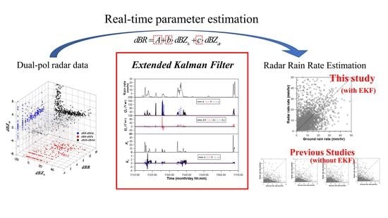
:The extended Kalman filter is an extended version of the Kalman filter for a non-linear problem. This study applies this extended Kalman filter to the real-time estimation of the parameters of the dual-pol radar rain rate estimator. The estimated parameters are also compared with those based on the least squares method. As an application example, this study considers four storm events observed by the Beaslesan radar in Korea. The findings derived include, first, that the parameters of the radar rain rate estimator obtained by the extended Kalman filter are totally different from those by the least squares method. In fact, the parameters obtained by the extended Kalman filter are found to be more reasonable, and are similar to those reported in previous studies. Second, the estimated rain rates based on the parameters obtained by the extended Kalman filter are found to be similar to those observed on the ground. Even though the parameters estimated by applying the least squares method are quite different from previous studies as well as those based on the extended Kalman filter, the resulting radar rain rate is found to be quite similar to that based on the extended Kalman filter. In conclusion, the extended Kalman filter can be a reliable method for real-time estimation of the parameters of the dual-pol radar rain rate estimator. The resulting rain rate is also found to be of sufficiently high quality to be applicable for other purposes, such as various flood warning systems.
1. Introduction
Significant advances in the field of hydrology have been made by introducing the meteorological radar [1]. In particular, high-resolution continuous systematic data are of great use in rainfall-runoff analysis [2]. The distributed rainfall-runoff model can directly use this systematic data for various analyses, such as flood inundation and flash flood [3,4,5]. This trend is the same in Korea, where flash floods in mountain areas with steep and complex terrain structure are of serious concern [6]. For the radar rain rate to secure more accurate quality, the use of radar data must be located at the center of the flash flood warning system [7].
Radar rain rate is estimated by analyzing the reflected electro-magnetic wave (i.e., reflectivity) from the rain drops within the atmosphere. Generally, a power function is used to convert the radar reflectivity into the radar rain rate. The so-called Z-R relation (i.e., Z = ARb) of the single-pol radar is to link the horizontal reflectivity (Z) and the ground rain rate (R). Z = 200R1.6 by Marshall and Palmer (1948) is one of the most famous equations of this kind [8]. However, the two parameters A and b are found to vary locally, as well as to depend on the storm type [9]. Generally, these parameters are determined by analyzing the observed data from both radar and rain gauge, which is one of the key parts of quantitative precipitation estimation (QPE).
Many studies have been conducted on parameter estimation of the Z-R relation. Most fundamental studies are based on the analysis of drop size distribution (DSD), whose result could directly be used to estimate the parameters [8,10,11,12,13]. It is also possible to find other studies to estimate the parameters directly by analyzing the radar reflectivity and rain gauge data. For example, Harter (1990) determined the parameters statistically based on the concept of least squares [14]. Rosenfeld et al. (1994) proposed a probability matching method (PMM) by comparing corresponding two cumulative probability distributions, those of radar reflectivity and ground rain rate [15].
However, the variation of DSD was another cause of preventing the optimal estimation of the parameters. Basically, it was impossible to determine a unique set of parameters for a given region, or even for a given storm event. The parameters vary storm by storm [16], and even change much within a single storm event [17,18,19]. It is also possible that the DSD can change within the atmosphere due to various reasons, such as collision and evaporation [20,21,22]. The simple application of a given Z-R relation can, thus, produce a significant number of errors in the estimation of the rain rate. In fact, this is a reason why real-time parameter estimation of the Z-R relation has been tried for operational radar rain rate estimation [23,24,25,26,27,28].
There have been many studies on the real-time parameter estimation of the Z-R relation [7,20,21,22,29,30,31,32]. For example, Kotarou et al. (1995) proposed real-time estimation of parameter A (after fixing parameter b) of the Z-R relation to remove the mean-field bias of the radar rain rate in Japan [31]. A similar approach was also applied to the radar QPE in Korea [22]. Rendon et al. (2011; 2013) also reported a similar approach of real-time estimation of parameter A around the South Florida Water Management District (SFWMD) [20,21]. On the other hand, Alfieri et al. (2010) estimated both parameters at the same time, and evaluated them for different temporal resolutions from 1 to 24 h [7]. Obviously, more stable (i.e., smoothly changing) parameters could be obtained when considering longer temporal resolution.
Interestingly, most of these studies were limited to the single-pol radar. Even for the dual-pol radar, the previous studies considered only the horizontal reflectivity due to its dynamic range wider than other variables [7,20,21]. This was mainly due to the fact that the effect of the horizontal reflectivity is large even in the dual-pol radar [33]. Additionally, limiting the number of parameters by two could make the problem simpler. Furthermore, even though the problem is for the real-time estimation of the parameters, the Kalman filter has never been considered. This might be due to the radar rain rate estimator being a power function, a non-linear function. Simply put, it cannot be directly applied to the Kalman filter. On the other hand, the Kalman filter has been a popular tool applied for the real-time estimation of the G/R ratio, i.e., the problem of mean-field bias correction [34,35,36,37,38,39]. The G/R ratio is estimated by the ratio between the ground rain rate (G) and the radar rain rate (R) [35,37]. The G/R ratio is generally modeled by a linear autoregressive model [18,21,36,40].
The purpose of this study is to evaluate the application of the extended Kalman filter for the real-time estimation of the parameters of the dual-pol radar rain rate estimator. In fact, the extended Kalman filter is an extended version of the Kalman filter for a non-linear problem. In principle, the problem for the dual-pol case is the same as that for the single-pol case. However, due to the increase of the number of parameters, the problem becomes a bit more complicated. As more parameters are involved, their reasonable estimation can be a key issue, especially when this kind of optimization technique is applied. As an example, this study considers the storm events observed by the Beaslesan radar in Korea.
2. Methodology
2.1. Rain Rate Estimator of the Dual-Pol Radar
The dual-pol radar collects and analyzes the radar echo from the rain drops within the atmosphere to produce various radar parameters. These radar parameters are also directly used to estimate the rain rate, which is called the quantitative rain rate estimation. The relation between the rain rate and the radar parameters is used in this step, which is called the rain rate estimator. The rain rate estimator is generally derived by statistically analyzing the rain rate data observed on the ground, and the radar parameters derived by the radar. The horizontal reflectivity, differential reflectivity, and specific differential phase are among those frequently used in those rain rate estimators. The quality of a rain rate estimator is, thus, dependent on the selected radar parameters.
This study considers the rain rate estimator based on the horizontal reflectivity and the differential reflectivity. This type of rain rate estimator is the most general one for the S-band dual-pol radar. As a type of power function, the rain rate estimator contains three parameters α, b, and c, which are generally determined before its application to the operation purpose:
where R represents the rain rate [mm/h], Zh is the horizontal reflectivity [mm6/m3], and Zdr is the differential reflectivity [no dimension]. R, Zh, and Zdr can also be represented using the dB (decibel) unit, which is based on the log-transformation, i.e., dBZ = 10log10(Z).
After the first attempt by Chandrasekar and Bringi (1988) [41], many studies of parameter estimation have been reported. The results of these studies also vary, depending on the geographical location and storm type. However, most of the estimated parameters are found to be within a narrow range. For example, parameter A, which is the log-tranformed α, has been estimated to be around −20, and parameter b to be around 0.9. Additionally, more than one half of the parameter estimation results provide parameter c to be around −1. Table 1 summarizes all the parameters from a total of 11 previous cases.
2.2. Kalman Filter
Kalman (1960) proposed a methodology for a real-time forecasting method based on the assumption of a linear system [53]. This so-called Kalman filter, once built by analyzing all available data up to the time point k-1, can produce an optimal sequential estimator from the following time point k. It is no longer necessary to analyze the entire data again to renew the filter, even though a new observation is provided. Additionally, as the whole procedure is expressed in the time domain, the Kalman filter is known to be easy to follow and handle. This is one reason why the Kalman filter has become so popular in the problem of real-time correction and forecasting [54,55].
The Kalman filter is based on the state-space model, which is composed of a system equation and a measurement equation [56]. In the case that a time series model is given, it should also be transformed into a state–space model. First, the system equation is a linear equation expressing the state vector xk at the current time step k by the state vector xk−1 at the previous time step k−1 and the white noise wk. That is:
where is a transition matrix to transform the state vector xk−1 into xk. The white noise wk is assumed to follow the Gaussian distribution with its mean zero and covariance Qk.
As the state vector xk cannot be directly observed in a real problem, a measurement equation is necessary. The measurement equation also linearly links the state vector xk and the measurement vector yk, along with another white noise vk [53]:
where Hk is a transition matrix to transform the state vector xk into the measurement vector yk and vk is also assumed to follow the Gaussian distribution with its mean zero and covariance Rk.
The principle of the Kalman Filter is to estimate the state variable using the error information about the predicted and the new measurement. When a new measurement is collected, the state variable is revised by comparing the uncertainty levels of the prediction and the measurement. The revised state variable is then used as the initial value for the prediction of the state variable at the next time step [35,57]. The uncertainty levels of the prediction and the measurement are summarized by the system error covariance Qk and the measurement error covariance Rk.
The state-space model can be derived using the time series model for the measurements of the state variable. The system error covariance and the measurement error covariance can also be derived using the time series model. The structure of the time series model, as well as the model parameters, including the residual variance, affect the error covariance of the state-space model. The derived state-space model is directly used for the Kalman filter application.
The Kalman filter is a set of mathematical equations (Table 2). These Kalman filter equations include a prediction of the state variable, an update of the error covariance of the predicted value, a calculation of the Kalman gain, an optimal estimation of the state variable, and an update of the error covariance of the optimal estimate, which are repeated at every time step [53,57]. Here, the negative sign (−) indicates the previous step before the update and the positive sign (+) the next step after the update.
Among these Kalman filter equations, the Kalman gain is very noticeable. Table 2 shows that the Kalman gain is related to the state estimate error covariance and the measurement error covariance. That is, the Kalman gain is a weighting factor deciding the relative weights of the state estimate and the measurement to decide the new state estimate. The Kalman gain also plays a key role balancing the uncertainty of the prediction and the measurement. The Kalman gain, as in Table 2, reflects the change of the state estimate error covariance Pk(−) and the measurement error covariance Rk. The state estimate error covariance Pk(−) is also dependent upon the system error covariance Qk. In the case that the system error covariance Qk is large, the state estimate error covariance Pk(−) also becomes large, leading to the Kalman gain being close to 1.0. On the other hand, in the case that the measurement error covariance Rk is large, as Rk becomes larger than Qk, indicating the uncertainty of measurement is larger than that of the system estimate, the Kalman gain approaches 0.0. That is, a higher state uncertainty should lead to a larger Kalman gain, and hence, a bigger update. In this case, the new measurement dominates the state estimates in the next time step. More detailed information about the Kalman filter can be found in Kalman (1960), Gelb (1974), and Box et al. (2015) [53,56,57].
2.3. Extended Kalman Filter
As the Kalman filter was originally developed based on the assumption of a linear system, an additional modification is necessary to apply it to a nonlinear system. Schmidt (1970) proposed a methodology for this purpose, called the extended Kalman filter, which is based on a linearization of the given nonlinear system (Simon, 2006) [58,59]. For example, the general form of the nonlinear state-space model is expressed as follows:
where uk is a controlling input vector, which is considered if needed. Both the system equation f(xk, uk) and the measurement equation h(xk) are nonlinear, and need to be transformed to be linear. In most studies, the Jacobian matrix is used as a linearization method. The Jacobian matrix is especially useful when the system is defined to be partial differentiable. The Jacobian matrices of the nonlinear functions f(xk, uk) and h(xk) are as follows:
Equations (6) and (7) represent the linearization procedure of the nonlinear system equation and the nonlinear measurement equation. The resulting Fk and Hk are assumed to be transition matrices of the linear system and measurement equations. Even though the linearization procedure is introduced in the extended Kalman filter, its theoretical background is exactly the same as that of the Kalman filter. The linearization procedure is simply to transform the relation between the independent variable and the dependent variable to be linear, to make the Kalman filter applicable. Table 2 also compares the Kalman filter and the extended Kalman filter.
3. Derivation of the Model
3.1. State-Space Model for Dual-Pol Radar Rain Rate Estimator
This study referred to Adamowski and Muir (1989) for the derivation of the state-space model [60]. They showed an example case for the single-pol radar rain rate estimator. The system equation was assumed to follow a random walk, and the measurement equation was made to follow the structure of the logarithmically transformed rain rate estimator. The error covariance matrix of the system equation was determined by the parameters of the rain rate estimator, while that of the measurement equation was updated every time step.
This study used the same idea of Adamowski and Muir (1989) to develop the state-space model for the rain rate estimator of the dual-pol radar [60]. In more detail, first, the basic equation form of the rain rate estimator of the dual-pol radar is given by Equation (1). By taking 10log10 of both sides, a new linear equation can be obtained in decibel (dB):
where dBR, dBZh, and dBZdr are the measurement variables, while A, b, and c are the state variables.
The system equation is assumed to be a random walk, which is as follows:
where xk is a state vector at time step k and wk is a system error following the Gaussian distribution with its mean zero and covariance Qk. Equation (9) can also be represented by a matrix form, which is directly applied to the Kalman filter:
where wA, wb, and wc represent the error of the state variables A, b, and c. The error covariance matrix is composed of the variances , , and and co-variances , , and of the state variables A, b, and c. That is:
The measurement equation is derived from Equation (5). First, the measurement dBR is expressed by a function of state variables A, b, and c as follows:
where vk represents the error term following the Gaussian distribution with its mean zero and covariance Rk. The function h(A, b, c)k, a function of state variables A, b, and c, is given as follows:
The function h(A, b, c)k transforms the state variable in the measurement equation into the measurement variable dBR. The Jacobian matrix is used as a transition Hk, which is nothing but the partial derivative of the function h(A, b, c)k by the state variables A, b, and c. The Jacobian matrix of Equation (13) is derived as follows:
Finally, the measurement equation is derived as follows:
The above equation considers the derived transition matrix, state variables, and measurement error.
3.2. Error Covariance and Initial Condition of the Extended Kalman Filter
In the application of the Kalman filter, the error covariance and the initial condition should be determined beforehand. In particular, appropriate determination of the error covariance of the system equation and that of the measurement equation is a key step for the successful application of the Kalman filter [61,62,63,64]. This may also be the most difficult step in the application of the Kalman filter [65]. It is, thus, not surprising that many studies have focused on this issue.
A practical method can be found in Wang et al. (1987), which assumed the error covariance of the system equation to be the mean square difference between the observed and the simulated [66]. Several other studies applied an adaptive algorithm to consider the uncertainty in the estimation of the error covariance at the current time step [67]. Their method was based on Sage and Husa (1969), where the error covariance in the previous time step was additionally considered in the estimation of the error covariance at the present time step [68]. Francois et al. (2003) proposed a slightly different method, which assumed that the error covariance was defined as the variation of the measurement [69]. The variation of the measurement was quantified by the error covariance of the measurement time series.
In fact, the error covariance is determined differently according to the methods mentioned above. In fact, the method used in this study is basically similar to Sage and Husa (1969) [68]. This method was advantageous, as the size of the data was big. Additionally, the update of the error covariance in this study was done by considering the variation of the state variable and measurement during the last five steps, which was available without any computation burden. Hence, the method used in this study may also be similar to that of Francois et al. (2003) [69].
The initial condition required for the Kalman filter application is the state variable , error covariance of the state estimate P0, measurement error covariance R0, and system error covariance Q0. First, the initial condition of the state variable was assumed to be the parameters proposed by Chandrasekar and Bringi (1988) [41]. This initial condition is one of the most popular options to be considered. Second, the uncertainty of the state variable was assumed to be the variance of the parameter determined based on the least squares method.
4. Application, Results, and Discussion
4.1. Study Area and Data
4.1.1. Radar and Rain Gauges Located at Study Area
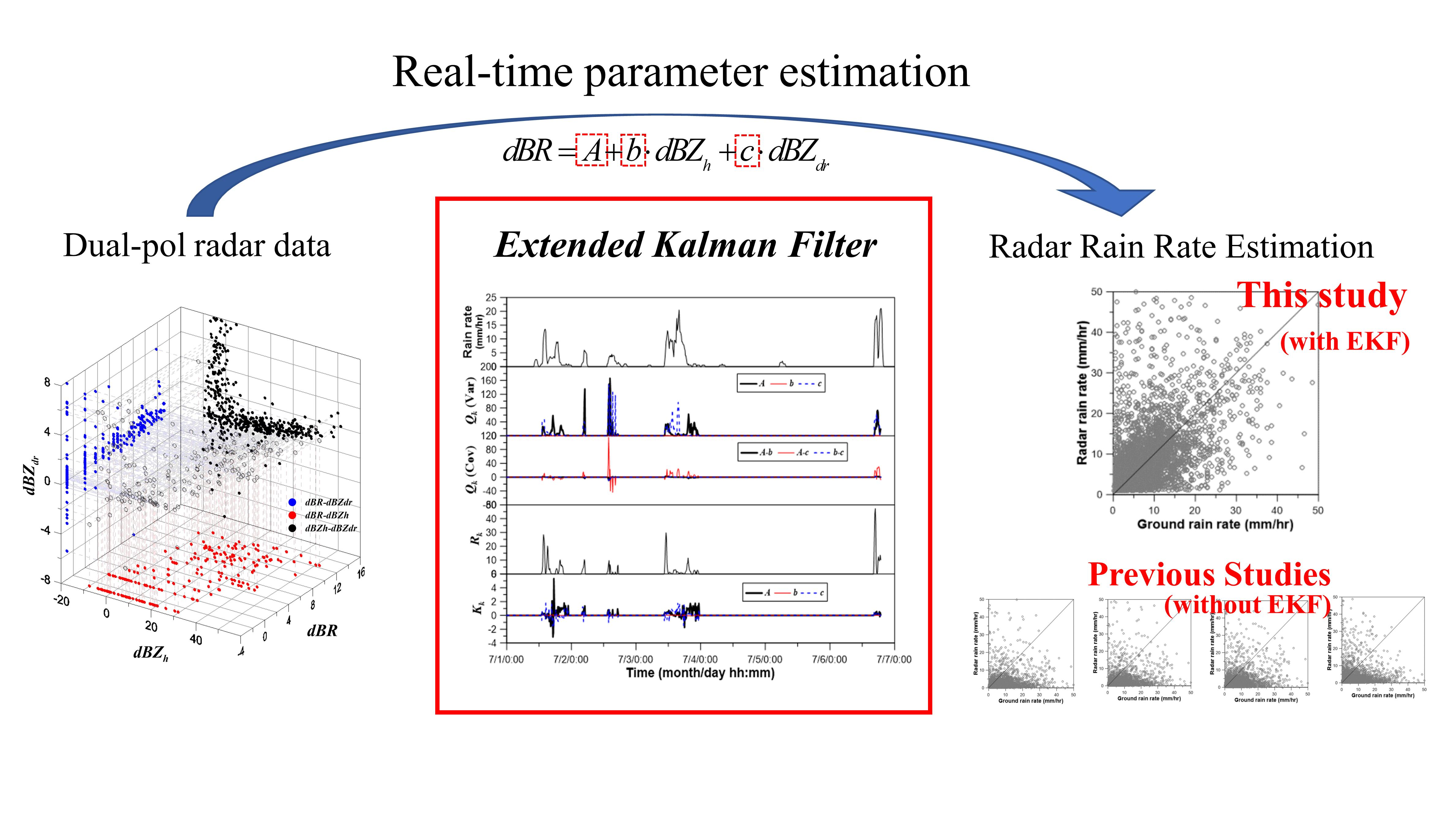
This study used the data collected by the Beaslesan radar in Korea. As a dual-pol S-band radar located at the top of Mt. Beaslesan (El. 1057 m), it was introduced in 2009. This radar covers the southern part of the Korean Peninsula. After three years of test operation, the data collected by the Beaslesan radar were opened to the public. During the dry period, the Beaslesan radar watches the area within a 250 km radius, but when rain drops are detected, the observation area is narrowed down to a 100 km radius. The beam width is 0.95°, and the lowest observation angle ranges (−0.5 to 1.59°), mainly due to different terrain blockage. This study also used this lowest angle data. The temporal resolution of the radar data is 2.5 min, and the spatial resolution is 125 m × 125 m. Figure 1 provides the location of the Beaslesan radar, along with its observation range.
The rain gauge data used in this study are those collected by 10 automatic weather stations (AWSs) located within a 100 km radius from the Beaslesan radar. These rain gauges are located at Gayasan (No. 311), Jinyoung (No. 673), Sunsan (No. 806), Euiheung (No. 807), Hwangseong (No. 811), Gimchun (No. 822), Hwabuk (No. 841), Dooseo (No. 900), Danjang (No. 922), and Shinpo (No. 936). Figure 1 also shows the locations of these 10 rain gauges. These rain gauges have produced the 1 min data since early 1990s, except the Gayasan and Jinyoung rain gauges, which were introduced in 2001 and 2009, respectively. The rain gauge data can be obtained from the data center of the Korean Meteorological Administration [70].
4.1.2. Rain Gauge and the Corresponding Radar Data for the Storm Events Used in This Study
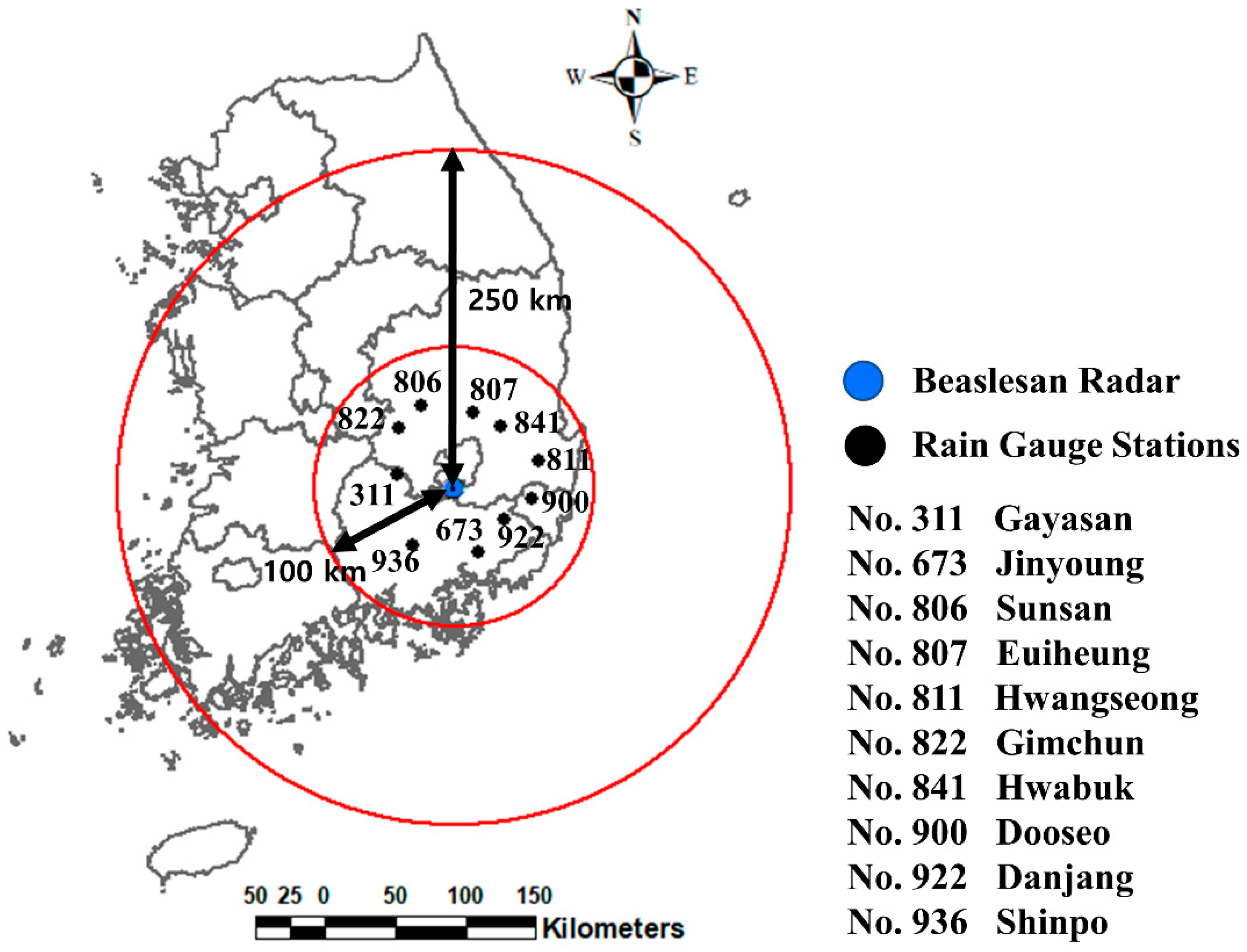
In this study, relatively long rainfall events were selected to show the advantage of using the extended Kalman filter. After reviewing the various rainfall events observed, this study selected four events occurred in 2016, 2018, 2019, and 2020. These rainfall events lasted for at least three days; additionally, the rainfall amount of each event was rather large. Figure 2 shows the time series of ground rainfall data, averaged with 10 AWS measurements and accumulated for every 10 min. Additionally, the basic statistics of these four events are summarized in Table 3. The events in 2016 and 2020 were frontal, and the events in 2018 and 2019 were caused by a typhoon. The event in 2019 was very intense, with a total rainfall of 203.9 mm and a maximum rain rate of 22.8 mm/h recorded on October 2 (22:00). On the other hand, the event in 2020 lasted four days, with a total rainfall of just 167.8 mm. In this study, the time interval of the data was set to be 10 min for both the rain gauge and the radar data.
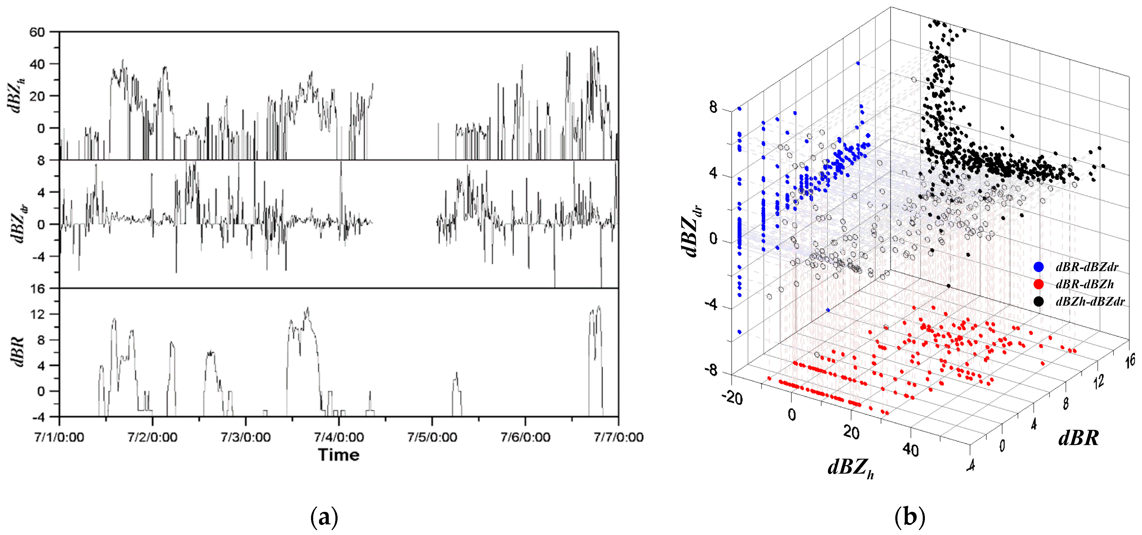
Figure 3 shows the time series plots and scatter plots of rain rate data collected at the Shinpo rain gauge (No. 936) in 2016, and radar data collected at the same location. The radar data include the horizontal reflectivity and the differential reflectivity, and the unit of data is dB (decibel). As can be seen in the time series plots (Figure 3a), the horizontal reflectivity in the dB unit (i.e., dBZh) ranges about (−10–50), while the differential reflectivity (i.e., dBZdr) ranges about (−8–8). The range of the rain rate in the dB unit (i.e., dBR) is about (−4–14). The data concentration around the −3 dBR value is mainly due to the minimum detectable rain rate of the rain gauge being 0.5 mm/h. The trend of dBR was found to be similar to that of dBZh, but when the rain rate was high, dBZdr seemed to approach zero.
Figure 3b shows that a somewhat weak but positive relation could be found between dBZh and dBR. The theoretically obvious positive relation was not so clear in this scatter plot, as the variation was too high. On the other hand, the relation between dBZdr and dBR was more obvious. That is, as dBR increases, dBZdr seems to converge to zero; but when dBR is rather low, the variation was still high. In fact, this relation was also found in other studies, such as Lee (2006), Chen et al. (2017), and Gou et al. (2019) [48,71,72]. The relation between dBZdr and dBZh was more interesting. A very strong and positive correlation could be found between dBZdr and dBZh. When removing the variation where dBZh is around zero, their relation seems very solid. The reason for this strong correlation could be explained by the positive relation between rainfall intensity and the characteristics of the raindrops (i.e., the drop size and drop shape). As dBZh increases from 0 to 50, dBZdr moves from 0 to 1.5.
4.2. Case of Shinpo Rain Gauge (No. 936) and the Corresponding Radar Data for the Event Occurred in 2016
4.2.1. Initial Condition and Result
For the rain gauge data collected at the Shinpo rain gauge (No. 936), the corresponding radar data were used in this application example. As the zero values for both rain rate and radar reflectivity could not be transformed into dB units, only the data pairs with positive values were considered in this application of the extended Kalman filter. Simply, in the case the rain rate is zero, the application of the extended Kalman filter was skipped.
The initial conditions of the state variable and state estimate error covariance P0 were set up as explained earlier. The initial conditions of the state variable were assumed to follow Chandrasekar and Bringi (1988) (i.e., A = −26.20, b = 0.94, and c = −1.08) [41], and that of the state estimate error covariance was assumed to be the error covariance of these three state variables estimated by applying the least squares method. The system error covariance Qk and the measurement error covariance Rk vary at every time step, whose values were determined by considering both the current and previous information. In this study, a total of six different datapoints (i.e., data collected at the previous five time steps and the current data) were considered in the estimation of the system and measurement error covariance.
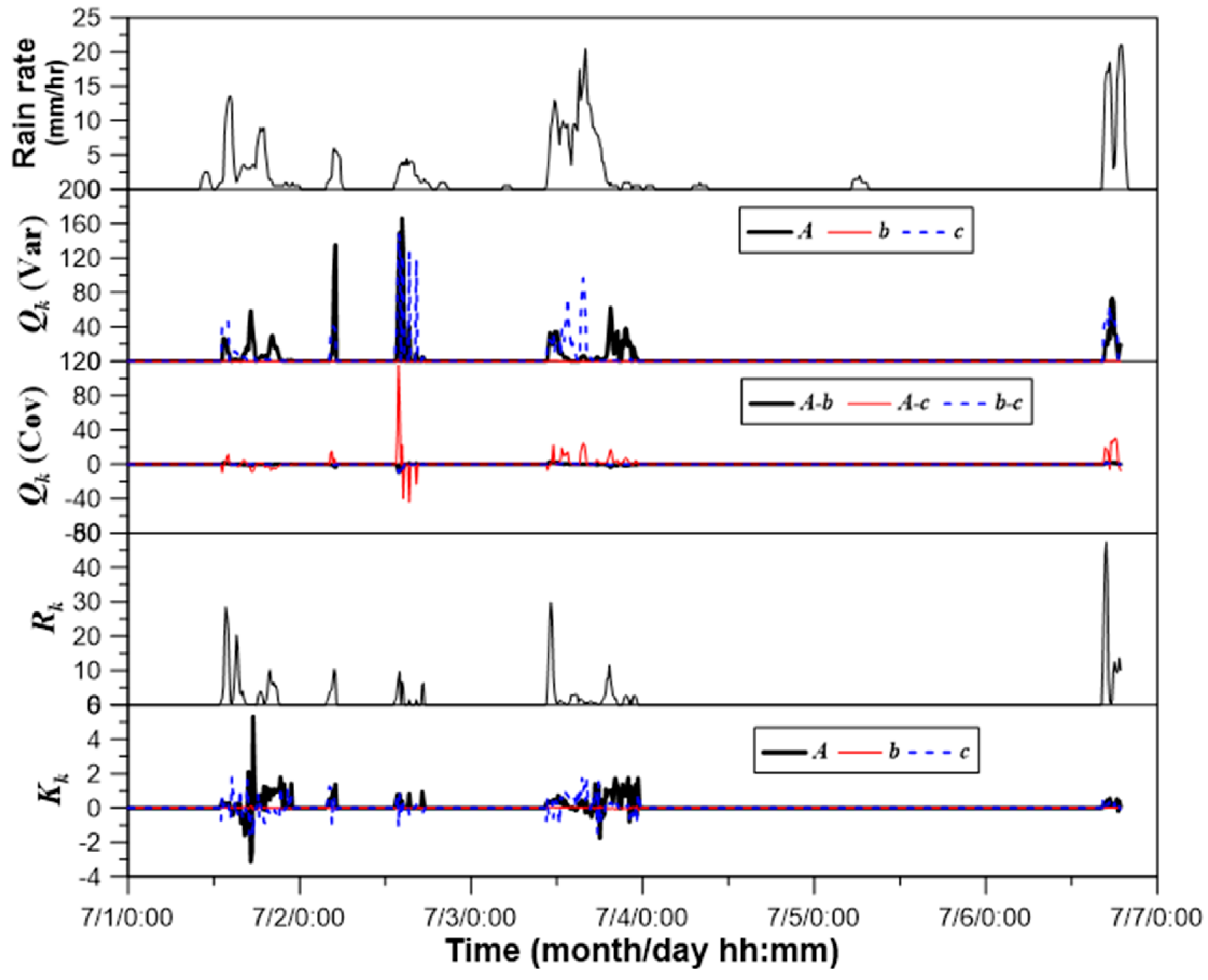
Figure 4 shows the temporal change of the variance-covariance of the state variable, variance of the measurement, and Kalman gain. First, the variance of parameter A was found to be much higher than that of parameters b and c. Obviously, the change of the estimate of parameter A was also much higher than those of parameters b and c. This change was also found to be dependent on the rain rate measured on the ground. This dependency is especially clear where the change of rain rate was rather high. The variance and covariance of the parameters sharply increased as the rain rate became higher, and decreased fast as the rain rate became smaller. On the other hand, the change of the variance-covariance became unnoticeable where the rain rate remained steady. The variability of the ground rain rate is considered in the estimation of measurement error variance, whose trend is also similar to the ground rain rate. This result indicates how the variance of the rain rate measured on the ground affects the Kalman gain, and ultimately the state variable estimate. The Kalman gain of parameter A was determined to be close to 1.0; on the other hand, those of parameters b and c were estimated to be near 0.0.
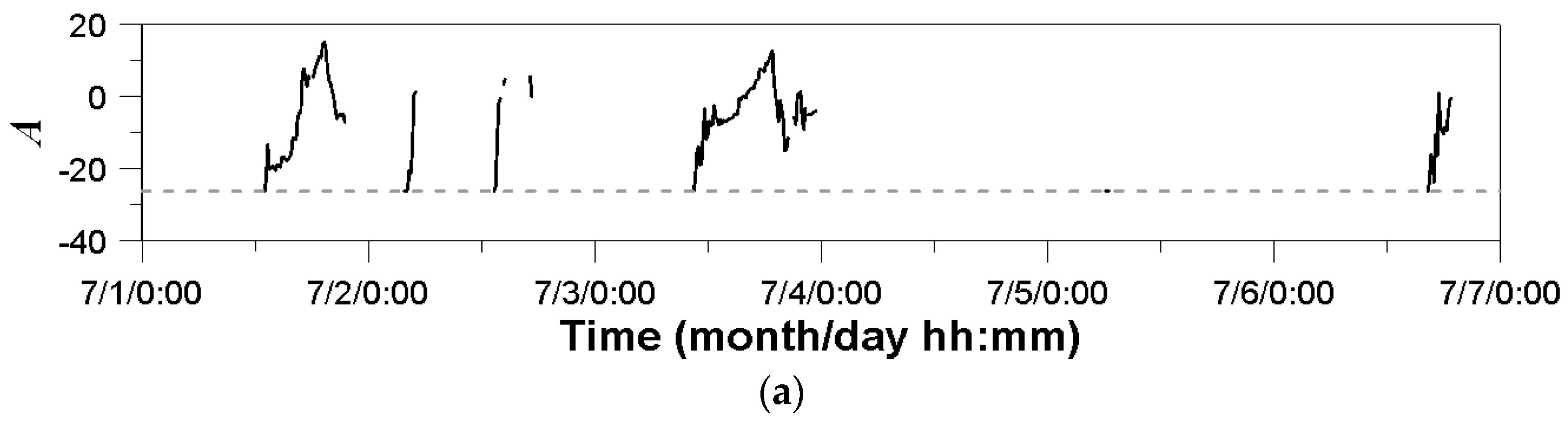
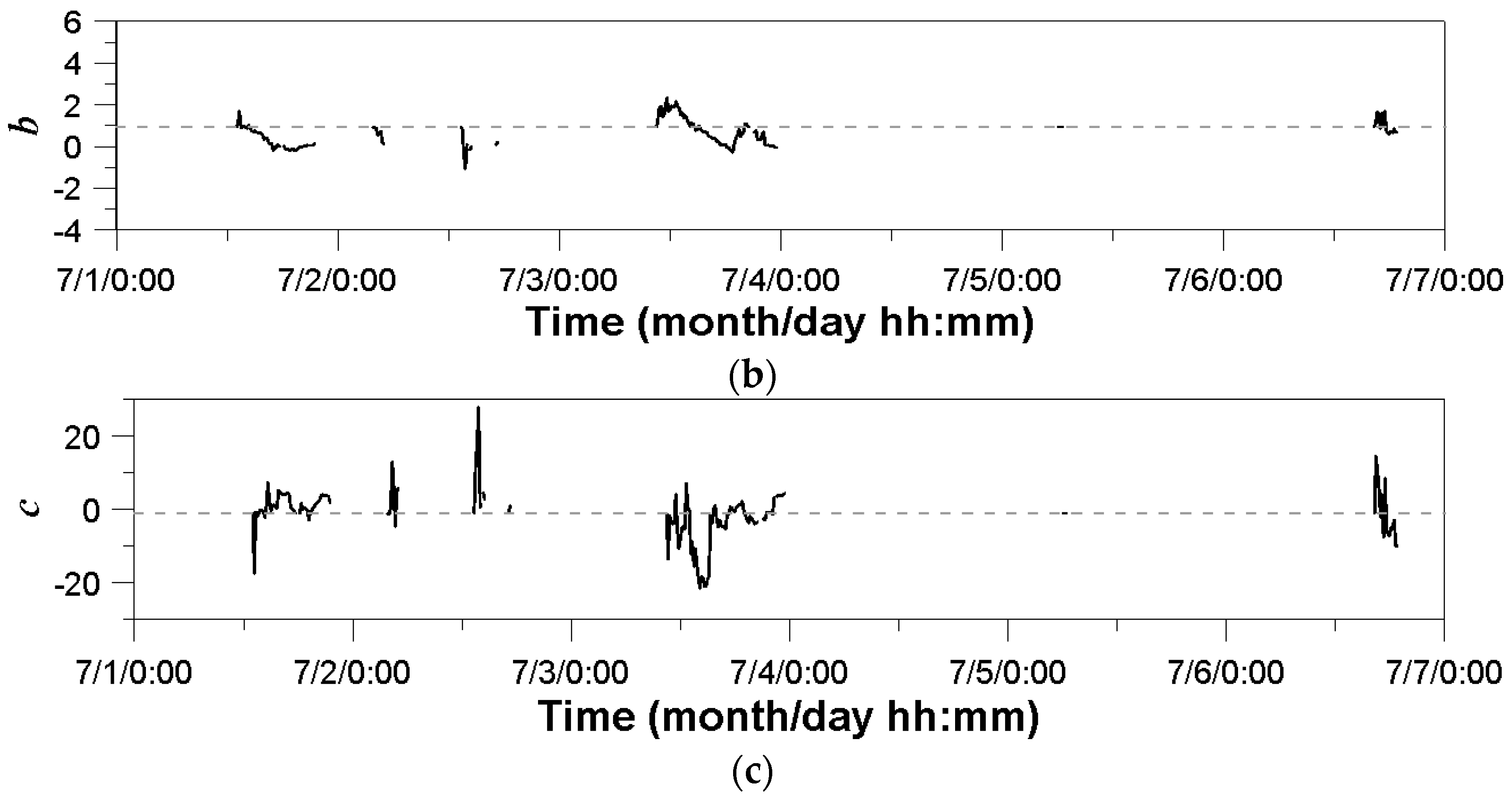
Figure 5 shows the real-time estimation result of parameters. First, the dashed horizontal line in Figure 5 represents the initial condition of the parameters based on Chandrasekar and Bringi (1988) [41]. Whenever the rainfall is newly detected after the rain ends, the same initial condition was repeatedly applied in this example case. The parameters vary over the period of the application example. In particular, the variation of parameter A was found to be higher than those of the other two parameters. Some studies have reported a divergence in the estimation of state variables [73,74,75], but that did not occur in this study. The estimates of these state variables were all found to be within reasonable ranges to confirm the stable application of the extended Kalman filter in this study.
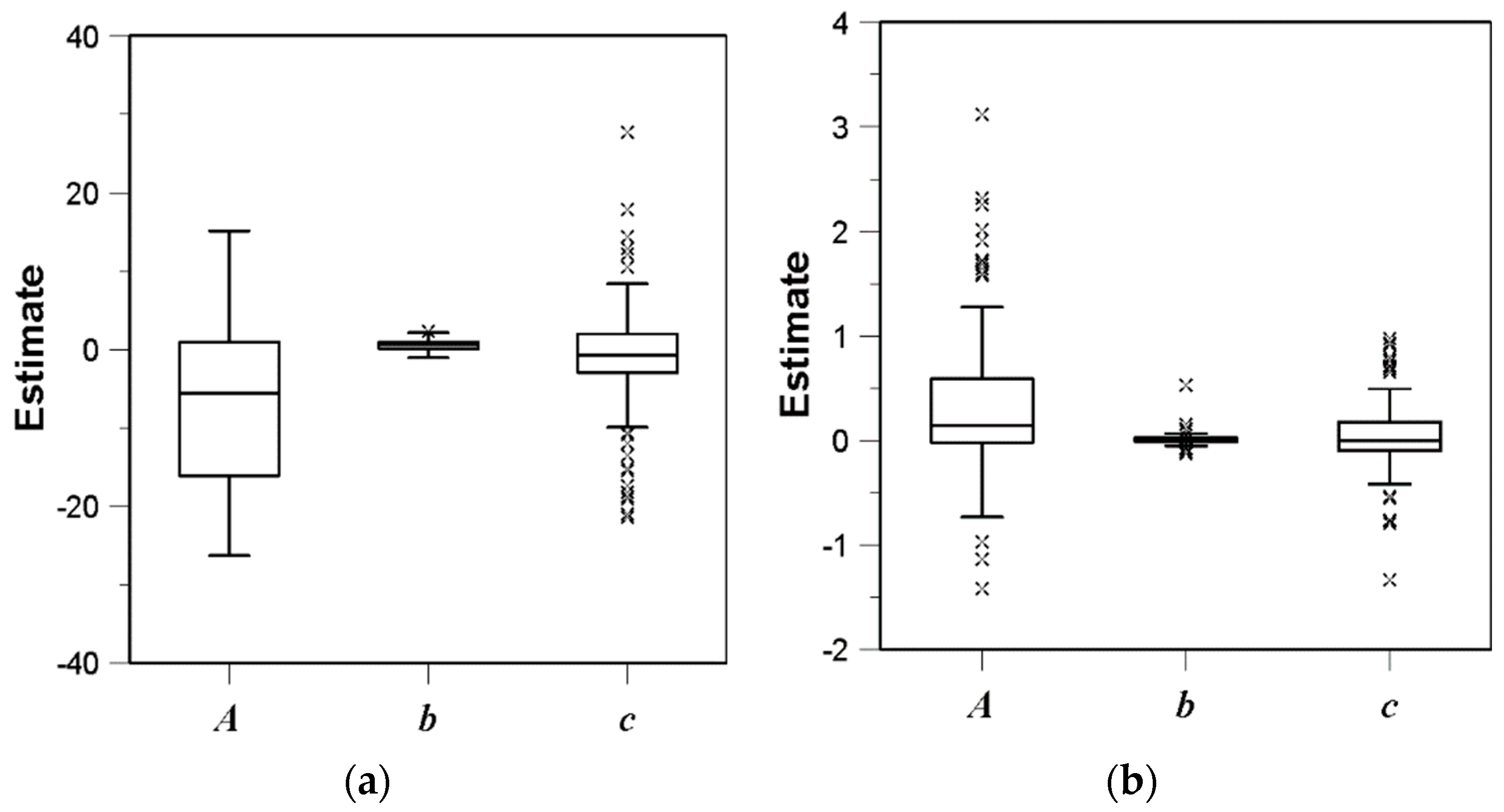
Additionally, this study compared the parameter estimates with their box-whisker plots (Figure 6a). The range of parameter A was larger than those of parameters b and c; on the other hand, the number of outliers of parameter c was found to be larger than those of the other two parameters. Parameters A and c seemed to be much affected by the large variation of rain rate. In fact, this result was also directly related to the Kalman gain determined (Figure 6b). The box-whisker plots of the three Kalman gains corresponding to the three parameters show exactly the same characteristics of the three parameters. The variation of the Kalman gain for parameter A was highest, while those for parameters b and c were smaller.
4.2.2. Comparison with the Least Squares Method
The application result of the extended Kalman filter was compared with the conventional least squares method. The least squares method may be the most common method for parameter estimation of the rain rate estimator [42,44,76,77]. The same least squares method was also applied in real time to the same data in this study, whose result was then compared with that of the extended Kalman filter. Exactly the same data under the same condition were considered in the estimation of the parameters based on the least squares method. The only difference in the application of the least squares method is the amount of data considered in the real-time application. That is, only the data during the previous one hour (i.e., 6 data) were considered in the application of the extended Kalman filter, but somewhat longer data during the previous three hours (i.e., 18 data) were considered in the application of the least squares method. This was simply to reserve a sufficient amount of data to make the application of the least squares method stable. As more data were used for the application of the least squares method, it might have some advantage over the application of the extended Kalman filter.
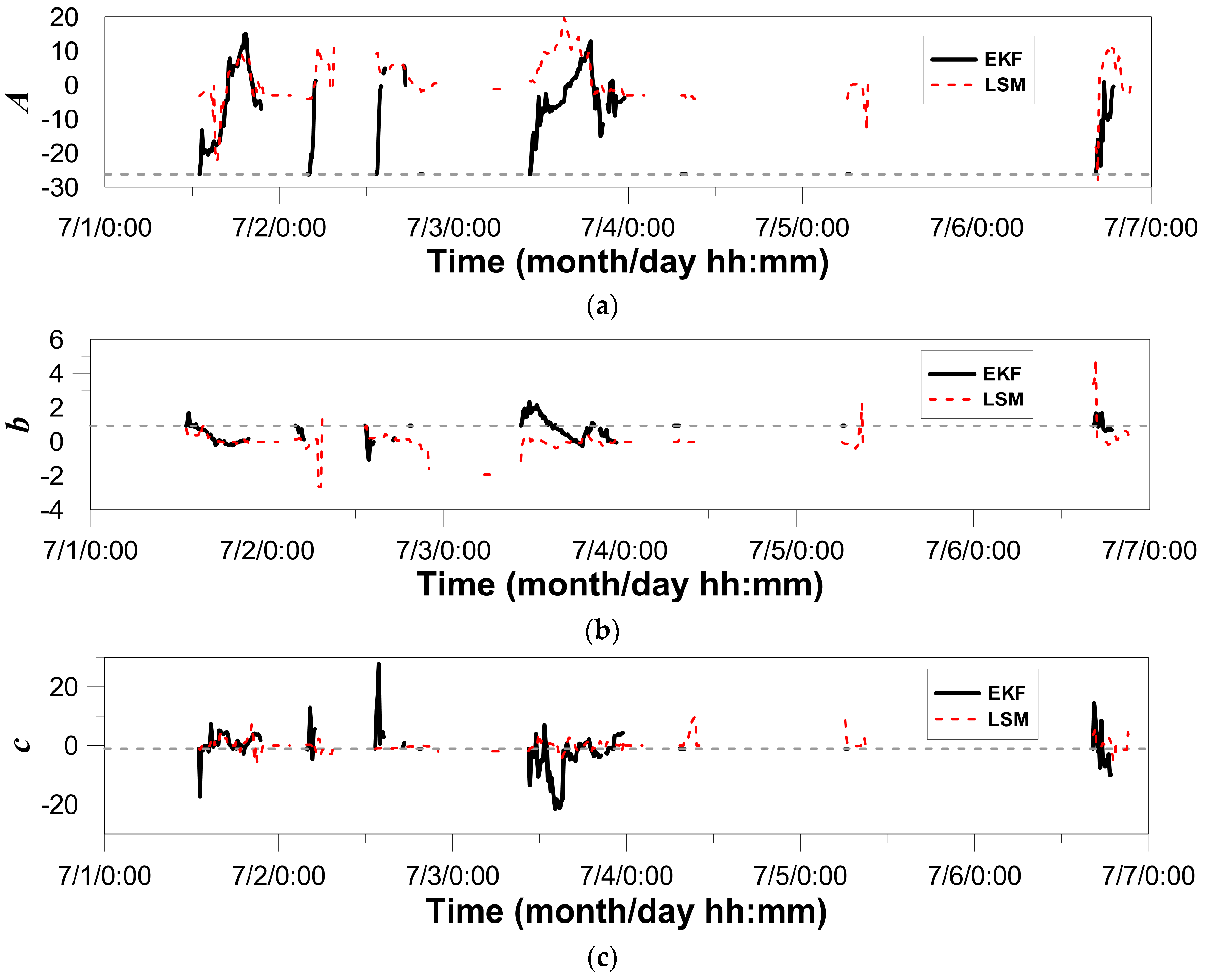
Figure 7 compares the behavior of the parameters estimated by applying the extended Kalman filter, and that by applying the least squares method. In this figure, the horizontal dashed line represents the initial condition [41], the same as in Figure 5. First of all, the variation of the parameters based on the extended Kalman filter was found to be higher than that based on the least squares method. In particular, the difference of parameter A was large. Parameter A, estimated by the least squares method, was found to be far out of the reasonable range based on previous studies (Table 1). It was the same for parameter b. Only the estimate of parameter c was somewhat similar to those in the previous studies.
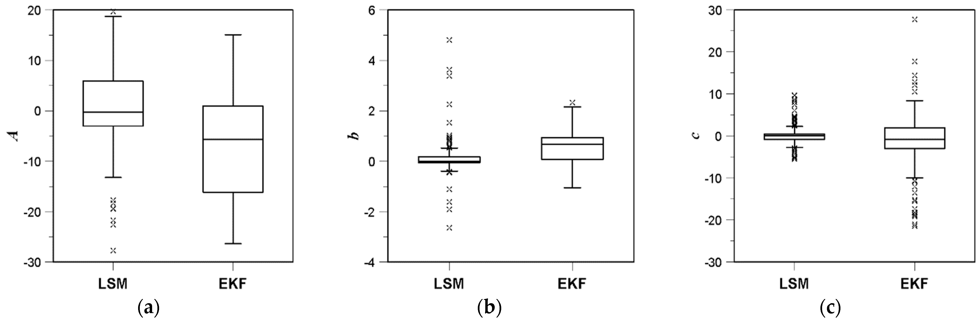
The difference of the parameters estimated by these two different methods can also be summarized by the box-whisker plot (Figure 8). The range of parameter A based on the least squares method was around (−5–5); on the other hand, the range based on the extended Kalman filter was around (−20–0). The range of parameter b based on the least squares method was around (0–0.2), but the range based on the extended Kalman filter was around (0.2–1.0). Additionally, the result of the paired T-test for each parameter also showed that the two parameter sets are very different. For example, the p-value of the paired T-test for the parameter A was less than 0.001 (t-value 13.03, n = 174). Similar result was also derived for the parameter b and c (p-value was less than 0.001 and 0.005, respectively).
Under the assumption that the parameters in Table 1 are rather reasonable, the parameters estimated by applying the extended Kalman filter seem to have more physical meaning. The parameters based on the least squares method are all out of the range of those in the previous studies. That is, the least squares method does not reproduce the physical parameters, but just an optimal set of parameters with minimum sum of differences between estimated and observed data.
The parameters A, b, and c are all affected by the rain drop shape and drop size; thus, they must have some physical meaning [78]. As the drop size increases, the shape becomes more horizontally oriented (i.e., the horizontal axis becomes longer than the vertical axis). As a result, the horizontal reflectivity becomes much stronger than the vertical reflectivity. As the rainfall intensity is proportional to the drop size, it is normal that the parameter b is positive (i.e., proportional to the horizontal reflectivity). On the other hand, the parameter c can be negative to consider the vertical reflectivity. In fact, the parameter c is the exponent of the differential reflectivity, which is the ratio of horizontal reflectivity to the vertical reflectivity. The parameters derived from the extended Kalman filter showed these physical characteristics clearer than those from the least squares method.
However, the variation of the parameters estimated by applying the extended Kalman filter was higher than those by applying the least squares method. This seems to be because the amount of data considered in the real-time estimation with the extended Kalman filter is smaller than that with the least squares method. Among those three parameters, the variation of parameter A was highest, while the other two parameters were smaller. The number of outliers was highest in the estimate of parameter c and smallest in the estimates of parameter A.
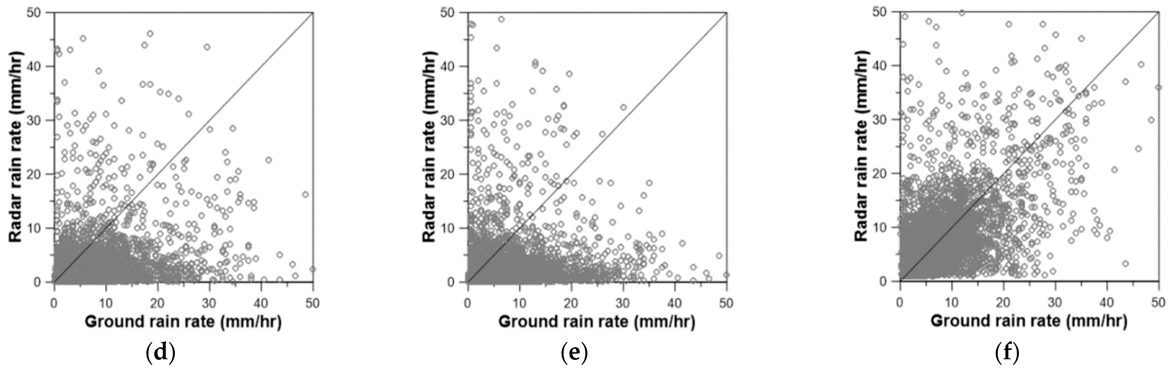
4.2.3. Radar Rain Rate vs. Ground Rain Rate
In this part of the study, the rain rate based on the estimated parameters by the extended Kalman filter were compared with that based on the parameters by the least squares method. Additionally, the rain rate estimated by applying the parameters in Chandrasekar and Bringi (1988), Chandrasekar (1990), Lee (2006), and Kwon et al. (2015) were considered in this comparison [41,43,48,51]. In particular, the parameters in Chandrasekar and Bringi (1988) are those used as initial conditions in the application of the extended Kalman filter [41].
Figure 9 shows the scatter plot that compares the ground rain rate with the radar rain rate estimated by applying the rain rate estimator. The radar rain rate varies depending on the parameters used, as mentioned in the previous paragraph. As the ground rain rate is the assumed truth, it must be better that the data points that are located around the one-to-one line. The amount of bias, as well as the randomness, can be evaluated by examining this scatter plot. For example, if the slope is far smaller than one, the radar rain rate is assumed to be underestimated. On the other hand, the overestimated radar rain rate will make the slope higher than one. Rather large deviation around the one-to-one line indicates instability of the radar rain rate. There could be various reasons, which in any event deteriorate the quality of radar data.
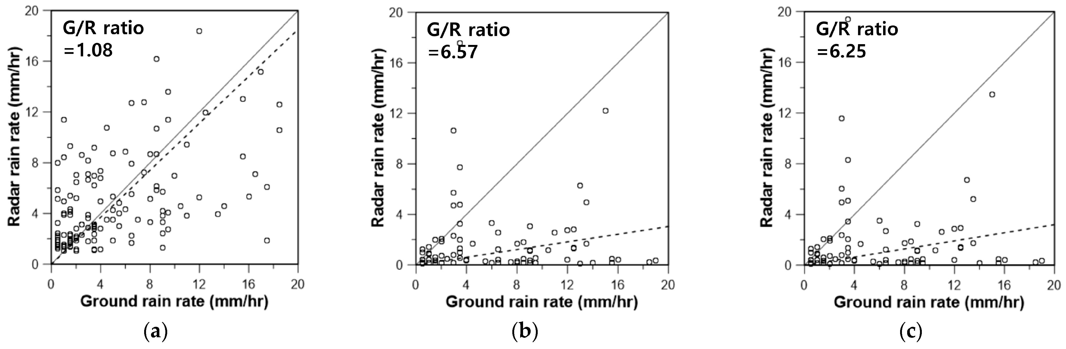
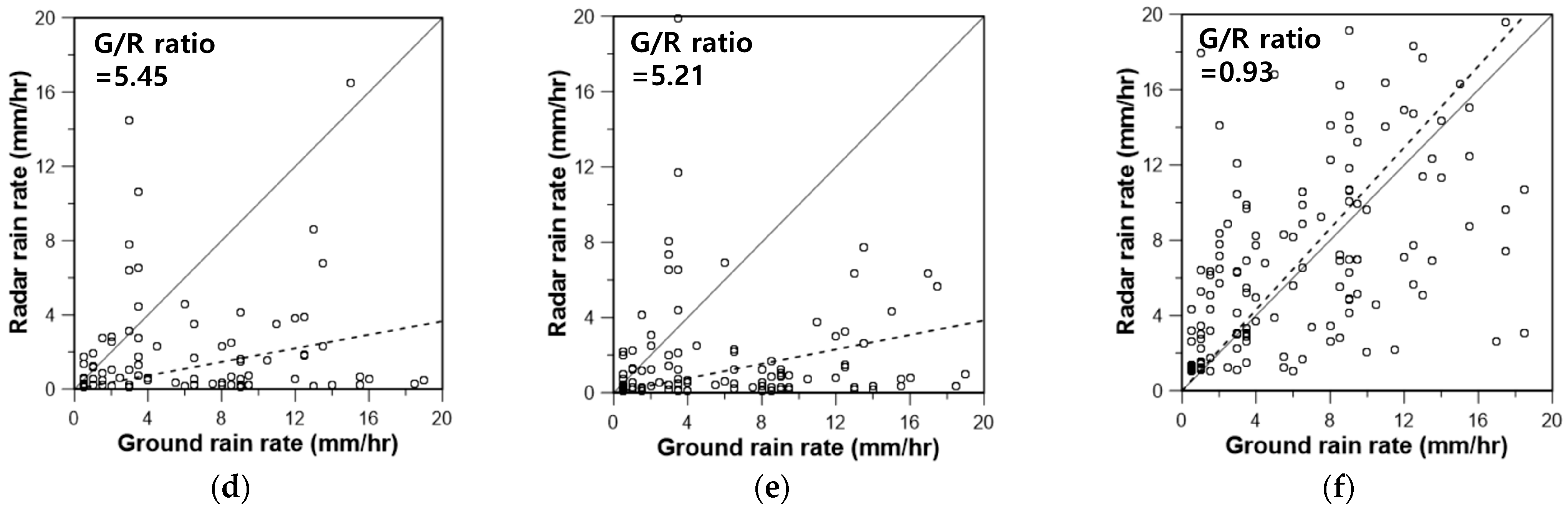
Figure 9 shows these problems of the radar rain rate. Most of the rain rate estimators provided underestimated values. In particular, the estimators in Chandrasekar and Bringi (1988) and Chandrasekar et al. (1990) provided smaller rain rates than those in Lee (2006) and Kwon et al. (2015) [41,43,48,51]. The rain rate estimator using the parameters based on the least squares method and the extended Kalman filter was much better than these four cases. In particular, the bias has been almost corrected to locate the pair of radar rain rate and ground rain rate around the one-to-one line However, the mean deviation from the one-to-one line was found to be much smaller in the application of the extended Kalman filter than that of the least squares method. Extremely deviated cases were also restricted in the application of the extended Kalman filter.
This difference can also be confirmed by comparing the so-called G/R ratio, which represents the ratio between the ground rain rate and the radar rain rate. The G/R ratio was 6.57 in the case where the radar rain rate estimator by Chandrasekar and Bringi (1988) was applied, and 6.25 in the case where the one by Chandrasekar et al. (1990) was applied [41,43]. It was somewhat smaller at 5.45 for Lee (2006), and 5.21 for Kwon et al. (2015) [48,51]. However, when the radar rain rate estimator based on the least squares method was applied, the G/R ratio became much smaller at 0.93. Finally, the G/R ratio estimated for the case of applying the extended Kalman filter was just 1.08. Obviously, this result emphasizes that real-time bias correction is still necessary, even in the application of the dual-pol radar. The difference can be significant, even in the case of using the conventional least squares method. However, much more advantage can be expected when using the extended Kalman filter. As already remarked in the previous section, the fact that the estimated parameter values using the extended Kalman filter could all lie within their reasonable ranges is another important advantage.
4.3. Case of Considering All Rain Gauges and the Corresponding Radar Data
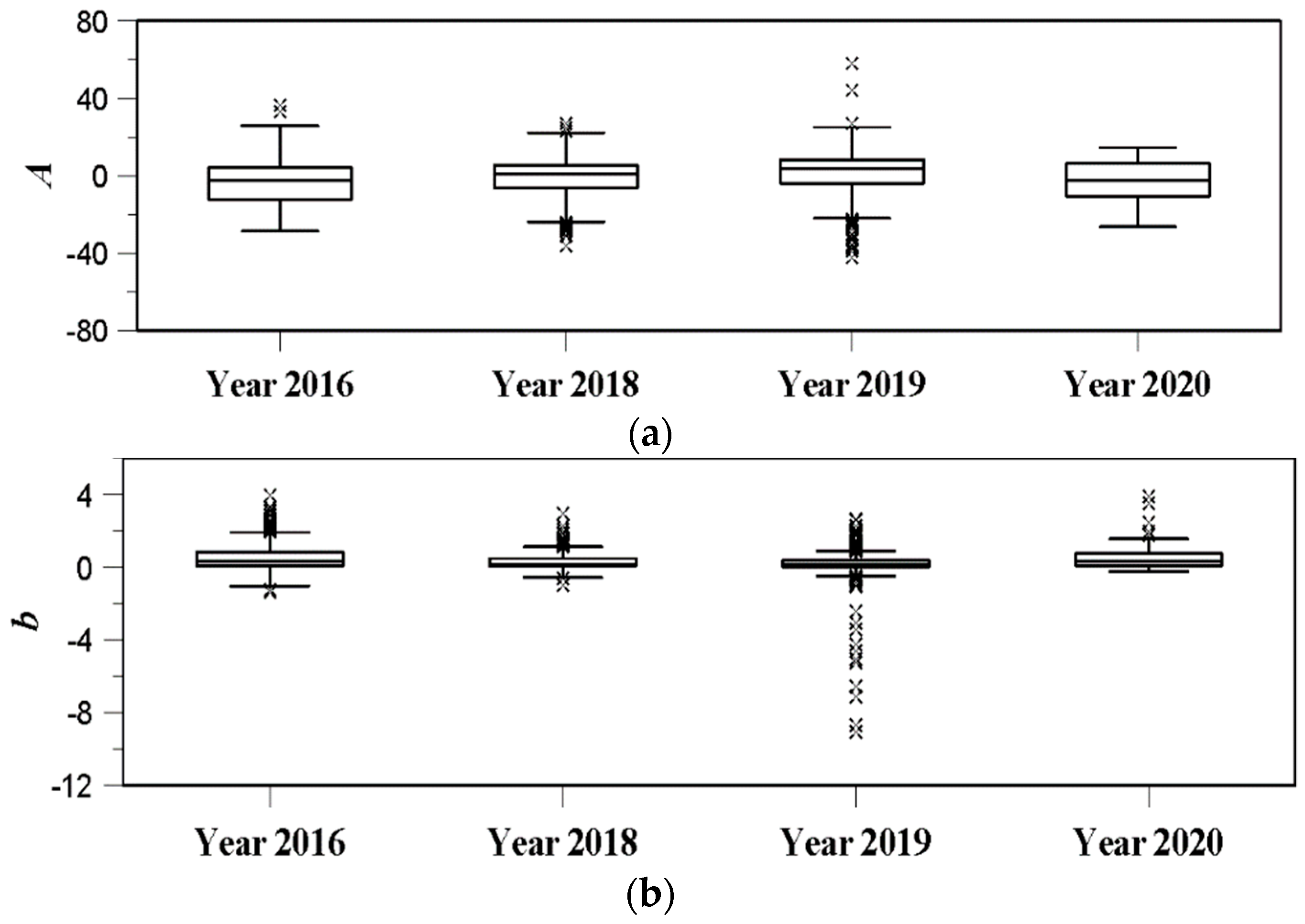
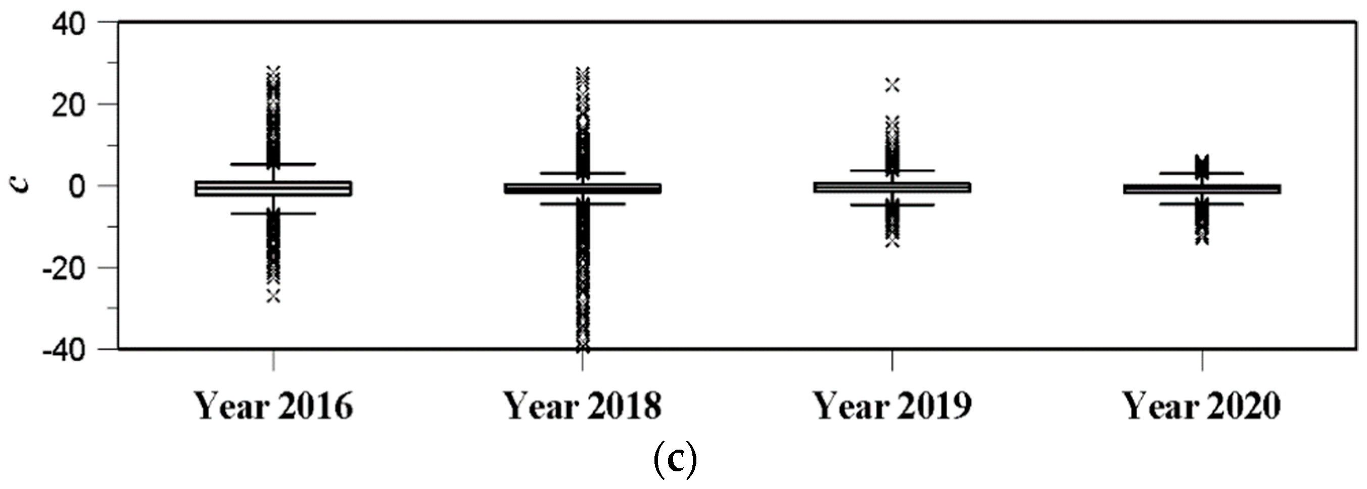
Figure 10 compares the result of parameter estimation using the extended Kalman filter for all rain gauges, including the Shinpo rain gauge (No. 936). The result of parameter estimation for four storm events was summarized by box-whisker plot. First, the application of the extended Kalman filter provided similar results in all AWS locations. Parameter A was estimated to be within the range (−25–5). Parameter b was within the range (0.2–1.2), and parameter c was within the range (−3–0). These results are very similar to those in Table 1. However, it was also noticeable that parameter c had rather many outliers compared with parameters A and b. If comparing the rainfall events, the interquartile range of the parameters for the rainfall events in 2016 and 2020 was found to be relatively wide with just a few outliers. The rainfall events in these years were longer and milder than the other two years. That is, the rainfall events in 2018 and 2019 were rather small but intense. As a result, the derived box-whisker plot showed a rather small inter-quartile range but many outliers. The application result of the least squares method was also found to be similar to that in the previous section (the results are not included in this figure). Basically, the estimated parameters were all out of reasonable range, except for parameter c.
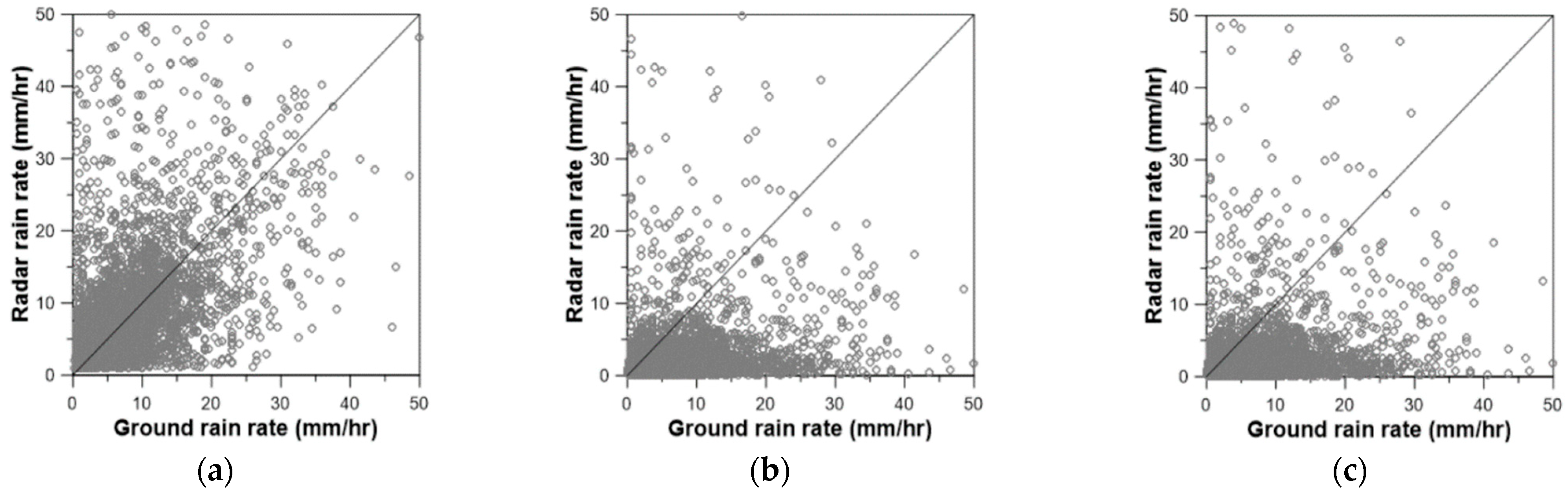
The estimated parameters were then applied to the radar rain rate estimator to estimate the rain rate, which were also compared with those based on the least squares method and other radar rain rate estimators. The data considered in Figure 11 are all 10 AWS locations, including Shinpo (No. 936), for four storm events. The comparison result was basically the same as that of the Shinpo rain gauge (No. 936) only. The comparison results with the radar rain rate estimator by Chandrasekar and Bringi (1988), Chandrasekar et al. (1990), Lee (2006), and Kwon et al. (2015) showed an underestimation problem [41,43,48,51]. This underestimation problem was somewhat alleviated in the use of the least squares method and the extended Kalman filter. However, it was not easy to distinguish the quality of the application results of the extended Kalman filter from that of the least squares method. This result was, in fact, quite disappointing as the parameters estimated by the least squares method were all out of reasonable ranges. As the parameters in this study are non-linearly correlated, simple application of an optimization technique may result in somewhat meaningless parameters. It is ironic, however, that the application of meaningless parameters can produce a good-looking result. With the result that the extended Kalman filter gives somewhat reasonable ranges of the estimated parameters, the authors argue that the parameters estimated based on the extended Kalman filter are physical, as well as consistent with previous studies. This result could not be obtained by simply applying the least squares method.
The above results in Figure 11 can also be confirmed by deriving the G/R ratio. Table 4 summarizes the G/R ratios of those cases in Figure 11 for each storm event. First, the G/R ratio in the application of the extended Kalman filter was estimated to be 1.01, which indicates a good radar rate estimation. The G/R ratio in the application of the least squares method was estimated to be 1.02, which is similar to that of the extended Kalman filter, while those in the applications of Chandrasekar and Bringi (1988) and Chandrasekar et al. (1990) were higher than 4.0 [41,43]. Additionally, the G/R ratios in the applications of Lee (2006) and Kwon et al. (2015) were higher than 2.0 [48,51].
5. Summary and Conclusions
This study applied an extended Kalman filter for real-time estimation of the parameters of the dual-pol radar rain rate estimator. The extended Kalman filter is an extended version of the Kalman filter for a non-linear problem. Additionally, the dual-pol radar contains more parameters than the single-pol radar, which makes it a rather more complicated problem than the single-pol case. As more parameters are involved, their reasonable estimation can be a key issue, especially when this kind of optimization technique is applied. This study considered four storm events that were observed by the Beaslesan radar in Korea. The results are summarized as follows.
First, the state-space model for the dual-pol radar rain rate estimator was derived. In this study, the rain rate estimator based on the horizontal reflectivity and the differential reflectivity was considered. In the rain rate estimator, dBR, dBZh, and dBZdr were set to be measurement variables, while A, b, and c were set to be state variables. Additionally, the initial condition of the state variable was assumed to be the parameters proposed by Chandrasekar and Bringi (1988) [41]. The update of the error covariance in this study was made by considering the variation of the state variable and the measurement during the last five steps, which was available without any computation burden.
Second, the application results of the extended Kalman filter were found to be very different from those of the least squares method. All the parameters estimated by applying the extended Kalman filter were found to be similar to those reported in previous studies. However, the parameters based on the least squares method were all irrational, totally different from the previous studies. Basically, the least squares method produced a set of parameters with least root mean square error, not the physical parameters.
Third, the rain rates estimated by applying the parameters based on the extended Kalman filter were found to be superior to those based on the previous studies. The result showed an advantage of using the real-time estimated parameters. However, it was also found that the least squares method could produce similar quality rain rate data to those of the extended Kalman filter. This result was also confirmed by the comparison of the G/R ratios. This result was, in fact, somewhat disappointing from the fact that the application of meaningless parameters derived by an optimization technique could produce quite good rain rate data. However, it must be an important characteristic of a non-linear system. That is, there can be many different parameter sets which can produce the same result.
In conclusion, it was found that the extended Kalman filter can be a good method for real-time estimation of the parameters of the dual-pol radar rain rate estimator. In particular, the estimated parameters were all reasonable, which was the most important difference from those estimated by applying the least squares method parameter values for the radar rain rate estimator. The resulting rain rates based on the extended Kalman filter was also of sufficiently high quality to be applicable for flood warning systems.
Author Contributions
Data curation, W.N.; Formal analysis, W.N.; Methodology, C.Y.; Supervision, C.Y.; Visualization, W.N.; Writing—original draft, W.N. and C.Y.; Writing—review and editing, W.N. and C.Y. All authors have read and agreed to the published version of the manuscript.
Funding
This work was supported by the Korea Environment Industry & Technology Institute (KEITI) through the Water Management Research Program, funded by the Korea Ministry of Environment (MOE) (127559), and the National Research Foundation of Korea (NRF) grant funded by the Korea government (MSIT) (No. NRF-2021R1A5A1032433).
Institutional Review Board Statement
Not applicable.
Informed Consent Statement
Not applicable.
Data Availability Statement
Not applicable.
Conflicts of Interest
The authors declare no conflict of interest.
References
- Habib, E.; Malakpet, C.G.; Tokay, A.; Kucera, P.A. Sensitivity of streamflow simulation to temporal variability and estimation of Z-R relationships. J. Hydrol. Eng. 2008, 13, 1177–1186. [Google Scholar] [CrossRef]
- Legates, D.R. Real-time calibration of radar precipitation estimates. Prof. Geogr. 2000, 52, 235–246. [Google Scholar] [CrossRef]
- Michelson, D.B.; Koistinen, J. Gauge-radar network adjustment for the baltic sea experiment. Phys. Chem. Earth (B) 2000, 25, 915–920. [Google Scholar] [CrossRef]
- Brown, P.E.; Diggle, P.J.; Lord, M.E.; Young, P.C. Space-time calibration of radar rainfall data. J. Royal Stat. Soc. Appl. Stat. 2001, 50, 221–242. [Google Scholar] [CrossRef]
- Costa, M.; Alpuim, T. Adjustment of state space models in view of area rainfall estimation. Environmetrics 2010, 22, 530–540. [Google Scholar] [CrossRef] [Green Version]
- Yoo, C.; Ha, E.; Kim, B.; Kim, K.; Choi, J. Sampling error of areal average rainfall due to radar partial coverage. J. Korea Water Resour. Assoc. 2008, 41, 545–558. [Google Scholar] [CrossRef] [Green Version]
- Alfieri, L.; Claps, P.; Laio, F. Time-dependent Z-R relationship for estimating rainfall fields from radar measurements. Nat. Hazard. Earth Sys. Sci. 2010, 10, 149–158. [Google Scholar] [CrossRef] [Green Version]
- Marshall, J.S.; Palmer, W.M.K. The distribution of raindrop with size. J. Atmos. Sci. 1948, 5, 165–166. [Google Scholar] [CrossRef]
- Krajewski, W.F.; Smith, J.A. Radar hydrology: Rainfall estimation. Adv. Water Resour. 2002, 25, 1387–1394. [Google Scholar] [CrossRef]
- Twomey, S. On the measurement of precipitation intensity by radar. J. Meteorol. 1952, 10, 66–67. [Google Scholar] [CrossRef] [Green Version]
- Blanchard, D.C. Raindrop size distribution in Hawaiian rains. J. Meteorol. 1953, 10, 457–473. [Google Scholar] [CrossRef] [Green Version]
- Jones, D.M.A. Rainfall Drop-Size Distribution and Radar Reflectivity; Illinois State Water Survey: Champaign, IL, USA, 1956. [Google Scholar]
- Battan, L.J. Radar Observation of the Atmosphere; The University of Chicago Press: Chicago, IL, USA, 1973. [Google Scholar]
- Harter, R.M. An Estimation of Rainfall Amounts Using Radar-Derived Z-R Relationships. Master’s Thesis, Purdue University, West Lafayette, IN, USA, 1990. [Google Scholar]
- Rosenfeld, D.; Wolff, D.B.; Amitai, E. The window probability matching method for rainfall measurements with radar. J. Appl. Meteorol. 1994, 33, 682–693. [Google Scholar] [CrossRef] [Green Version]
- Steiner, M.; Smith, J.A. Reflectivity, rain rate, and kinetic energy flux relationships based on raindrop spectra. J. Appl. Meteorol. 2000, 39, 1923–1940. [Google Scholar] [CrossRef]
- Uijlenhoet, R.; Steiner, M.; Smith, J.A. Variability of raindrop size distributions in a squall line and implications for radar rainfall estimation. J. Hydrol. 2003, 4, 43–61. [Google Scholar] [CrossRef]
- Kim, J.; Yoo, C. Use of a dual Kalman filter for real-time correction of mean field bias of radar rain rate. J. Hydrol. 2014, 519, 2785–2796. [Google Scholar] [CrossRef]
- Kim, J.; Yoo, C.; Lim, S.; Choi, J. Usefulness of relay-information-transfer for radar QPE. J. Hydrol. 2015, 531, 308–319. [Google Scholar] [CrossRef]
- Rendon, S.H.; Vieux, B.E.; Pathak, C.S. Deriving radar specific Z-R relationships for hydrologic operations. In Proceedings of the World Environmental and Water Resources Congress 2011: Bearing Knowledge for Sustainability, Palm Springs, CA, USA, 22–26 May 2011; pp. 4682–4687. [Google Scholar]
- Rendon, S.H.; Vieux, B.E.; Pathak, C.S. Continuous forecasting and evaluation of derived Z-R relationships in a sparse rain gauge network using NEXRAD. J. Hydrol. Eng. 2013, 18, 175–182. [Google Scholar] [CrossRef]
- Jung, S.H.; Kim, K.E.; Ha, K.J. Real-time estimation of improved radar rainfall intensity using rainfall intensity measured by rain gauges. Asia-Pac. J. Atmos. Sci. 2005, 41, 751–762. [Google Scholar]
- Hudlow, M.D. Technological developments in real-time operational hydrologic forecasting in the United States. J. Hydrol. 1988, 102, 69–92. [Google Scholar] [CrossRef]
- Borga, M.; Anagnostou, E.N.; Frank, E. On the use of real-time radar rainfall estimates for flood prediction in mountainous basins. J. Geophys. Res. Atmos. 2000, 105, 2269–2280. [Google Scholar] [CrossRef]
- Young, C.B.; Bradley, A.A.; Krajewski, W.F.; Kruger, A.; Morrissey, M.L. Evaluating NEXRAD multisensor precipitation estimates for operational hydrologic forecasting. J. Hydrometeorol. 2000, 1, 241–254. [Google Scholar] [CrossRef] [Green Version]
- Krajewski, W.F.; Kruger, A.; Singh, S.; Seo, B.C.; Smith, J.A. Hydro-NEXRAD-2: Real-time access to customized radar-rainfall for hydrologic applications. J. Hydroinform. 2013, 15, 580–590. [Google Scholar] [CrossRef]
- Chen, H.; Chandrasekar, V. The quantitative precipitation estimation system for Dallas–Fort Worth (DFW) urban remote sensing network. J. Hydrol. 2015, 531, 259–271. [Google Scholar] [CrossRef] [Green Version]
- Krajewski, W.F.; Ceynar, D.; Demir, I.; Goska, R.; Kruger, A.; Langel, C.; Mantilla, R.; Niemeier, J.; Quintero, F.; Seo, B.; et al. Real-time flood forecasting and information system for the state of Iowa. Bull. Am. Meteorol. Soc. 2017, 98, 539–554. [Google Scholar] [CrossRef]
- Anagnostou, E.N.; Krajewski, W.F. Real-time radar rainfall estimation. Part I: Algorithm formulation. J. Atmos. Oceanic Technol. 1999, 16, 189–197. [Google Scholar] [CrossRef]
- Anagnostou, E.N.; Krajewski, W.F. Real-time radar rainfall estimation. Part II: Case study. J. Atmos. Oceanic Technol. 1999, 16, 198–205. [Google Scholar] [CrossRef]
- Kotarou, T.; Takumi, N.; Takaaki, Y. Operational calibration of raingauge radar by 10-minute telemeter rainfall. In Proceedings of the 3rd International Symposium on Hydrological Applications of Weather Radars, Sao Paulo, Brazil, 20–23 August 1995; pp. 75–81. [Google Scholar]
- Seo, B.C.; Krajewski, W.F.; Kruger, A.; Domaszczynski, P.; Smith, J.A.; Steiner, M. Radar-rainfall estimation algorithms of Hydro-NEXRAD. J. Hydroinform. 2011, 13, 277–291. [Google Scholar] [CrossRef]
- Schneebeli, M.; Berne, A. An extended Kalman filter framework for polarimetric X-band weather radar data processing. J. Atmos. Ocean. Technol. 2012, 29, 711–730. [Google Scholar] [CrossRef]
- Ahnert, P.R.; Krajewski, W.F.; Jonson, E.R. Kalman filter estimation of radar-rainfall field bias. In Proceedings of the 23rd Conference on Radar Meteorology, AMS, Boston, MA, USA, 22–26 September 1986; pp. JP33–JP37. [Google Scholar]
- Lin, D.S.; Krajewski, W.F. Recursive methods of estimating radar-rainfall field bias. In Proceedings of the 24th Radar Meteorology conference, Tallahassee, FL, USA, 27–31 March 1989; pp. 648–651. [Google Scholar]
- Smith, J.A.; Krajewski, W.F. Estimation of the mean field bias of radar rainfall estimates. J. Appl. Meteorol. 1991, 30, 397–412. [Google Scholar] [CrossRef] [Green Version]
- Lee, Y.H.; Singh, V.P. Application of the Kalman filter to the Nash model. Hydrol. Process. 1998, 12, 755–767. [Google Scholar] [CrossRef]
- Seo, D.J.; Breidenbach, J.P.; Johnson, E.R. Real-time estimation of mean field bias in radar rainfall data. J. Hydrol. 1999, 223, 131–147. [Google Scholar] [CrossRef]
- Yoo, C.; Kim, J.; Chung, J.H.; Yang, D.M. Mean field bias correction of the very short range forecast rainfall using the Kalman filter. J. Korean Soc. Hazard Mitig. 2011, 11, 17–28. [Google Scholar] [CrossRef] [Green Version]
- Chumchean, S.; Seed, A.; Sharma, A. Correcting of real-time radar rainfall bias using a Kalman filtering approach. J. Hydrol. 2006, 317, 123–137. [Google Scholar] [CrossRef]
- Chandrasekar, V.; Bringi, V.N. Error structure of multiparameter radar and surface measurements of rainfall. Part I: Differential reflectivity. J. Atmos. Oceanic Technol. 1988, 5, 783–795. [Google Scholar] [CrossRef] [Green Version]
- Aydin, K.; Zhao, Y.; Seliga, T.A. Rain-induced attenuation effects on C-band dual-polarization meteorological radars. Geosci. Remote Sens. Lett. 1989, 27, 57–66. [Google Scholar] [CrossRef]
- Chandrasekar, V.; Bring, V.N.; Balakrishana, N.; Zrnic, D.S. Error structure of multiparameter radar and surface measurements of rainfall. Part III: Specific differential phase. J. Atmos. Oceanic Technol. 1990, 7, 621–629. [Google Scholar] [CrossRef] [Green Version]
- Aydin, K.; Giridhar, V. C-band dual-polarization radar observables in rain. J. Atmos. Sci. 1992, 9, 383–390. [Google Scholar] [CrossRef] [Green Version]
- Gorgucci, E.; Chandrasekar, V.; Scarchilli, G. Radar and surface measurement of rainfall during CaPE: 26 July 1991 case study. J. Appl. Meteor. 1995, 34, 1570–1577. [Google Scholar] [CrossRef]
- Bringi, V.N.; Chandrasekar, V. Polarimetric Doppler Weather Radar, Principles and Applications; Cambridge University Press: New York, NY, USA, 2001. [Google Scholar]
- Ryzhkov, A.V.; Giangrade, S.E.; Schuur, T.J. Rainfall estimation with a polarimetric prototype of WSR-88D. J. Appl. Meteor. 2005, 44, 502–515. [Google Scholar] [CrossRef] [Green Version]
- Lee, G.W. Sources of errors in rainfall measurements by polarimetric radar: Variability of drop size distributions, observational noise, and variation of relationships between R and polarimetric parameters. J. Atmos. Oceanic Technol. 2006, 23, 1005–1028. [Google Scholar] [CrossRef]
- Cifelli, R.; Chandrasekar, V.; Lim, S.; Kennedy, P.C.; Wang, Y.; Rutledge, S.A. A new dual-polarization radar rainfall algorithm: Application in Colorado precipitation events. J. Atmos. Oceanic Technol. 2011, 28, 352–364. [Google Scholar] [CrossRef] [Green Version]
- WRC. Development and Application of Cross Governmental Dual-pol. Radar Harmonization; Weather Radar Center: Seoul, Korea, 2014. [Google Scholar]
- Kwon, S.; Lee, G.; Kim, G. Rainfall estimation from an operational S-band dual-polarization radar: Effect of radar calibration. J. Meteor. Soc. Japan. 2015, 93, 65–79. [Google Scholar] [CrossRef] [Green Version]
- Zhang, Y.; Liu, L.; Wen, H.; Wu, C.; Zhang, Y. Evaluation of the polarimetric-radar quantitative precipitation estimates of an extremely heavy rainfall event and nine common rainfall events in Guangzhou. Atmosphere 2018, 9, 330. [Google Scholar] [CrossRef] [Green Version]
- Kalman, R.E. A new approach to linear filtering and prediction problems. Trans. ASME J. Basic Eng. 1960, 82, 35–45. [Google Scholar] [CrossRef] [Green Version]
- Park, S.W. Real-Time Flood Forecasting by Transfer Function Types Model and Filtering Algorithm. Ph.D. Thesis, Dongguk University, Seoul, Korea, 1993. [Google Scholar]
- Jang, S.G. Combining Forecast Methods of Chungju Dam Streamflow using Kalman Filter. Master’s Thesis, Seoul National University, Seoul, Korea, 2002. [Google Scholar]
- Box, G.E.P.; Jenkins, G.M.; Reinsel, G.C.; Ljung, G.M. Time Series Analysis: Forecasting and Control; John Wiley & Sons: Hoboken, NJ, USA, 2015. [Google Scholar]
- Gelb, A. Applied Optimal Estimation; The MIT Press: Cambridge, MA, USA, 1974. [Google Scholar]
- Schmidt, S.F. Computational Techniques in Kalman filtering, in Theory and Applications of Kalman Filtering; NATO Advisory Group for Aerospace Research and Development: London, UK, 1970; Volume 139, pp. 219–292. [Google Scholar]
- Simon, D. Optimal State Estimation: Kalman, H Infinity, and Nonlinear Approaches; John Wiley & Sons: Hoboken, NJ, USA, 2006. [Google Scholar]
- Adamowski, K.; Muir, J. A Kalman filter modelling of space-time rainfall using radar and raingauge observations. Can. J. Civil Eng. 1989, 16, 767–773. [Google Scholar] [CrossRef]
- O’Connell, P.E.; Clarke, R.T. Adaptive hydrological forecasting—A review. Hydrolog. Sci. J. 1981, 26, 179–205. [Google Scholar]
- Hebson, C.; Wood, E.F. Partitioned state and parameter estimation for real-time flood forecasting. Appl. Math. Comput. 1985, 17, 357–374. [Google Scholar] [CrossRef]
- Seo, B.H.; Gang, G.W. A hydrologic prediction of streamflows for flood forecasting and warning system. J. Korea Water Resour. Assoc. 1985, 18, 153–161. [Google Scholar]
- Chou, C.M.; Wang, R.Y. Application of wavelet-based multi-model Kalman filters to real-time flood forecasting. Hydrol. Process. 2004, 18, 987–1008. [Google Scholar] [CrossRef]
- Eigbe, U.; Beck, M.B.; Hirano, W.F. Kalman filtering in groundwater flow modelling: Problems and prospects. Stoch. Hydrol. Hydraul. 1998, 12, 15–32. [Google Scholar] [CrossRef]
- Wang, G.T.; Yu, Y.S.; Wu, K. Improved flood routing by ARMA modelling and the Kalman filter technique. J. Hydrol. 1987, 93, 175–190. [Google Scholar]
- Wang, C.H.; Bai, Y.L. Algorithm for real time correction of stream flow concentration based on Kalman filter. J. Hydrol. Eng. 2008, 13, 290–296. [Google Scholar] [CrossRef]
- Sage, A.; Husa, G.W. Adaptive filtering with unknown prior statistics. In Proceedings of the Joint Automatic Control Conference, Washington, DC, USA, 7–9 May 1969; Volume 7, pp. 760–769. [Google Scholar]
- Francois, C.; Quesney, A.; Ottle, C. Sequential assimilation of ERS-1 SAR data into a coupled land surface-hydrological model using an extended Kalman filter. J. Hydrometeorol. 2003, 4, 473–487. [Google Scholar] [CrossRef]
- Korea Meteorological Administration KMA. 2019. Available online: http://www.data.kma.go.kr (accessed on 27 June 2019).
- Chen, H.; Lim, S.; Chandrasekar, V.; Jang, B.J. Urban hydrological applications of dual-polarization X-band radar: Case study in Korea. J. Hydrol. Eng. 2017, 22, E5016001. [Google Scholar] [CrossRef]
- Gou, Y.; Ma, Y.; Chen, H.; Yin, J. Utilization of a C-band polarimetric radar for severe rainfall event analysis in complex terrain over eastern China. Remote Sens. 2019, 11, 22. [Google Scholar] [CrossRef] [Green Version]
- Murty, Y.V.V.S.; Smolinski, W.J. Design and implementation of a digital differential relay for a 3-phase power transformer based on Kalman filtering theory. IEEE Trans. Power Del. 1988, 3, 525–533. [Google Scholar] [CrossRef]
- Leung, H.; Zhu, Z.; Ding, Z. An aperiodic phenomenon of the extended Kalman filter in filtering noisy chaotic signals. IEEE Trans. Signal Process. 2000, 48, 1807–1810. [Google Scholar] [CrossRef]
- Macias, J.A.; Gomez, A. Self-tuning of Kalman filters for harmonic computation. IEEE Trans. Power Del. 2006, 21, 501–503. [Google Scholar] [CrossRef]
- Sachidananda, M.; Zrnic, D.S. Rain rate estimates from differential polarization measurements. J. Atmos. Oceanic Technol. 1987, 4, 588–598. [Google Scholar] [CrossRef] [Green Version]
- Brandes, E.A.; Zhang, G.; Vivekanandan, J. Experiments in rainfall estimation with a polarimetric radar in a subtropical environment. J. Appl. Meteor. 2002, 41, 674–685. [Google Scholar] [CrossRef] [Green Version]
- Gorgucci, E.; Scarchilli, G.; Chandrasekar, V.; Bringi, V.N. Rainfall estimation from polarimetric radar measurements: Composite algorithms immune to variability in raindrop shape–size relation. J. Atmos. Oceanic Technol. 2001, 18, 1773–1786. [Google Scholar] [CrossRef]
Figure 1.
Location of Beaslesan radar in Korea and 10 rain gauges selected in this study within the radar umbrella.
Figure 1.
Location of Beaslesan radar in Korea and 10 rain gauges selected in this study within the radar umbrella.

Figure 2.
Time series plots of mean rain rate observed at 10 rain gauge stations located within the Beaslesan radar umbrella during (a) 1–6 July 2016, (b) 25–28 August 2018, (c) 1–3 October 2019, and (d) 22–25 July 2020.
Figure 2.
Time series plots of mean rain rate observed at 10 rain gauge stations located within the Beaslesan radar umbrella during (a) 1–6 July 2016, (b) 25–28 August 2018, (c) 1–3 October 2019, and (d) 22–25 July 2020.

Figure 3.
Time series plots and scatter plots of rain rate observed at the Shinpo rain gauge station (No. 936) for the storm event that occurred in 2016 and the corresponding radar data: (a) time series plots, (b) three-dimensional scatter plot.
Figure 3.
Time series plots and scatter plots of rain rate observed at the Shinpo rain gauge station (No. 936) for the storm event that occurred in 2016 and the corresponding radar data: (a) time series plots, (b) three-dimensional scatter plot.

Figure 4.
Rain rate, variance and covariance of state variables, measurement error covariance, and behavior of Kalman gain at the Shinpo rain gauge station (No. 936).
Figure 4.
Rain rate, variance and covariance of state variables, measurement error covariance, and behavior of Kalman gain at the Shinpo rain gauge station (No. 936).

Figure 5.
Resulting time series plots of parameters at the Shinpo rain gauge station (No. 936) estimated by applying the extended Kalman filter: (a) parameter A, (b) parameter b, (c) parameter c.
Figure 5.
Resulting time series plots of parameters at the Shinpo rain gauge station (No. 936) estimated by applying the extended Kalman filter: (a) parameter A, (b) parameter b, (c) parameter c.


Figure 6.
Box-whisker plots of the parameters and Kalman gains at the Shinpo rain gauge station (No. 936) estimated by applying the extended Kalman filter: (a) parameters, (b) Kalman gains.
Figure 6.
Box-whisker plots of the parameters and Kalman gains at the Shinpo rain gauge station (No. 936) estimated by applying the extended Kalman filter: (a) parameters, (b) Kalman gains.

Figure 7.
Comparison of time series plots of estimated parameters at the Shinpo rain gauge station (No. 936) by applying the extended Kalman filter (EKF) and the least squares method (LSM): (a) parameter A, (b) parameter b, (c) parameter c.
Figure 7.
Comparison of time series plots of estimated parameters at the Shinpo rain gauge station (No. 936) by applying the extended Kalman filter (EKF) and the least squares method (LSM): (a) parameter A, (b) parameter b, (c) parameter c.

Figure 8.
Comparison of box-whisker plots of the estimated parameters at the Shinpo rain gauge station (No. 936) by applying the extended Kalman filter (EKF) and the least squares method (LSM): (a) parameter A, (b) parameter b, (c) parameter c.
Figure 8.
Comparison of box-whisker plots of the estimated parameters at the Shinpo rain gauge station (No. 936) by applying the extended Kalman filter (EKF) and the least squares method (LSM): (a) parameter A, (b) parameter b, (c) parameter c.

Figure 9.
Comparison of the ground rain rate and radar rain rate at the Shinpo rain gauge station (No. 936) by applying the parameters of radar rain rate estimator in this study (EKF and LSM) and several other studies: (a) EKF, (b) Chandrasekar and Bringi (1988) [41], (c) Chandrasekar et al. (1990) [43], (d) Lee (2006) [48], (e) Kwon et al. (2015) [51], (f) LSM.


Figure 10.
Comparison of box plots for three estimated parameters at 10 rain gauge stations for four storm events by applying the extended Kalman filter: (a) parameter A, (b) parameter b, (c) parameter c.
Figure 10.
Comparison of box plots for three estimated parameters at 10 rain gauge stations for four storm events by applying the extended Kalman filter: (a) parameter A, (b) parameter b, (c) parameter c.


Figure 11.
Same as Figure 9, but for all 10 rain gauge stations of four storm events: (a) EKF, (b) Chandrasekar and Bringi (1988) [41], (c) Chandrasekar et al. (1990) [43], (d) Lee (2006) [48], (e) Kwon et al. (2015) [51], (f) LSM.


Table 1.
Various parameter sets of the dual-pol radar rain rate estimator reported worldwide.
| References | Parameters | ||
|---|---|---|---|
| A | b | c | |
| Chandrasekar and Bringi (1988) [41] | −26.20 | 0.94 | −1.08 |
| Aydin et al. (1989) [42] | −26.78 | 0.96 | −1.17 |
| Chandrasekar et al. (1990) [43] | −27.03 | 0.97 | −1.08 |
| Aydin and Giridhar (1992) [44] | −26.25 | 0.95 | −1.17 |
| Gorgucci et al. (1995) [45] | −20.00 | 0.92 | −0.37 |
| Bringi and Chandrasekar (2001) [46] | −21.74 | 0.71 | −3.43 |
| Ryzhkov et al. (2005) [47] | −17.99 | 0.74 | −1.03 |
| Lee (2006) [48] | −24.79 | 0.94 | −1.13 |
| Cifelli et al. (2011) [49] | −21.74 | 0.93 | −3.43 |
| WRC (2014) [50] | −20.91 | 0.91 | −4.25 |
| Kwon et al. (2015) [51] | −22.10 | 0.95 | −5.55 |
| Zhang et al. (2018) [52] | −20.76 | 0.93 | −0.41 |
Table 2.
Comparison of the Kalman filter and extended Kalman filter algorithms.
| Steps | Kalman Filter | Extended Kalman Filter |
|---|---|---|
| Initial values | , , , | , , , |
| State estimate prediction | ||
| State estimate error covariance prediction | ||
| Kalman gain | ||
| State estimate update | ||
| State estimate error covariance update | ||
Table 3.
Basic characteristics of the four storm events used in this study.
| No. | Duration | Type | Total Rainfall (mm) | Maximum Rainfall Intensity (mm/h) |
|---|---|---|---|---|
| 1 | 1–6 July 2016 | Frontal | 177.8 | 10.4 |
| 2 | 25–28 August 2018 | Typhoon | 190.1 | 13.1 |
| 3 | 1–3 October 2019 | Typhoon | 203.9 | 22.8 |
| 4 | 22–25 July 2020 | Frontal | 167.8 | 12.8 |
Table 4.
G/R ratios of the radar rain rate depending on different radar rain rate estimators.
| No. | Year | EKF | Chandrasekar and Bringi (1988) [41] | Chandrasekar et al. (1990) [43] | Lee (2006) [48] | Kwon et al. (2015) [51] | LSM |
|---|---|---|---|---|---|---|---|
| 1 | 2016 | 1.02 | 5.06 | 4.70 | 5.00 | 3.96 | 1.07 |
| 2 | 2018 | 1.04 | 3.08 | 2.91 | 2.34 | 1.23 | 0.95 |
| 3 | 2019 | 1.00 | 5.99 | 5.62 | 4.96 | 9.45 | 1.04 |
| 4 | 2020 | 0.97 | 3.77 | 3.67 | 2.75 | 1.85 | 1.04 |
| Mean | 1.01 | 4.27 | 4.02 | 3.48 | 2.48 | 1.02 | |
Publisher’s Note: MDPI stays neutral with regard to jurisdictional claims in published maps and institutional affiliations. |
© 2021 by the authors. Licensee MDPI, Basel, Switzerland. This article is an open access article distributed under the terms and conditions of the Creative Commons Attribution (CC BY) license (https://creativecommons.org/licenses/by/4.0/).
Share and Cite
MDPI and ACS Style
Na, W.; Yoo, C. Real-Time Parameter Estimation of a Dual-Pol Radar Rain Rate Estimator Using the Extended Kalman Filter. Remote Sens. 2021, 13, 2365. https://0-doi-org.brum.beds.ac.uk/10.3390/rs13122365
AMA Style
Na W, Yoo C. Real-Time Parameter Estimation of a Dual-Pol Radar Rain Rate Estimator Using the Extended Kalman Filter. Remote Sensing. 2021; 13(12):2365. https://0-doi-org.brum.beds.ac.uk/10.3390/rs13122365
Chicago/Turabian StyleNa, Wooyoung, and Chulsang Yoo. 2021. "Real-Time Parameter Estimation of a Dual-Pol Radar Rain Rate Estimator Using the Extended Kalman Filter" Remote Sensing 13, no. 12: 2365. https://0-doi-org.brum.beds.ac.uk/10.3390/rs13122365
Note that from the first issue of 2016, this journal uses article numbers instead of page numbers. See further details here.