
Insights from the P Wave Travel Time Tomography in the Upper Mantle Beneath the Central Philippines


Abstract
:
1. Introduction
2. Data and Methods
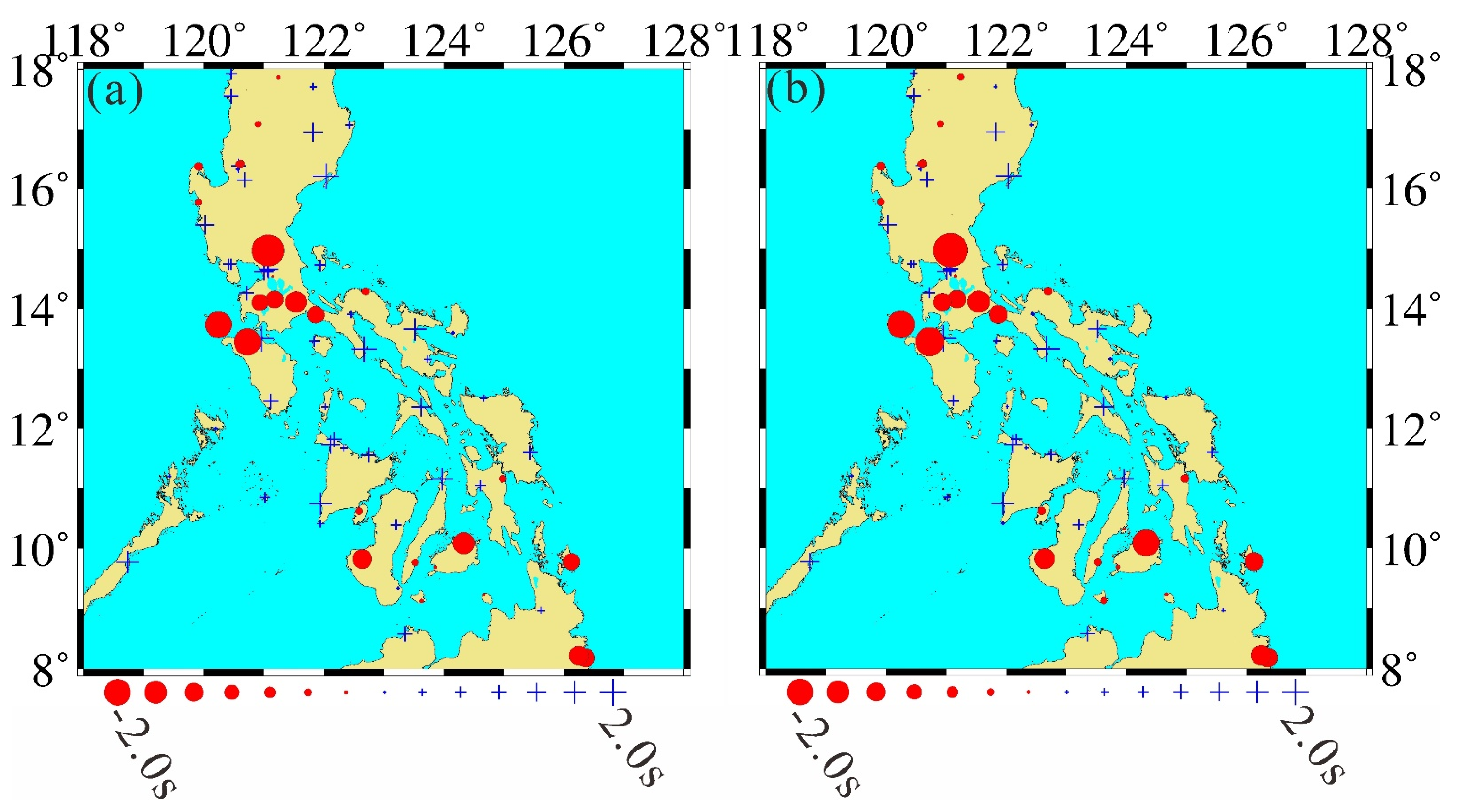
2.1. Data
2.2. Crust Correction
- (1)
- (2)
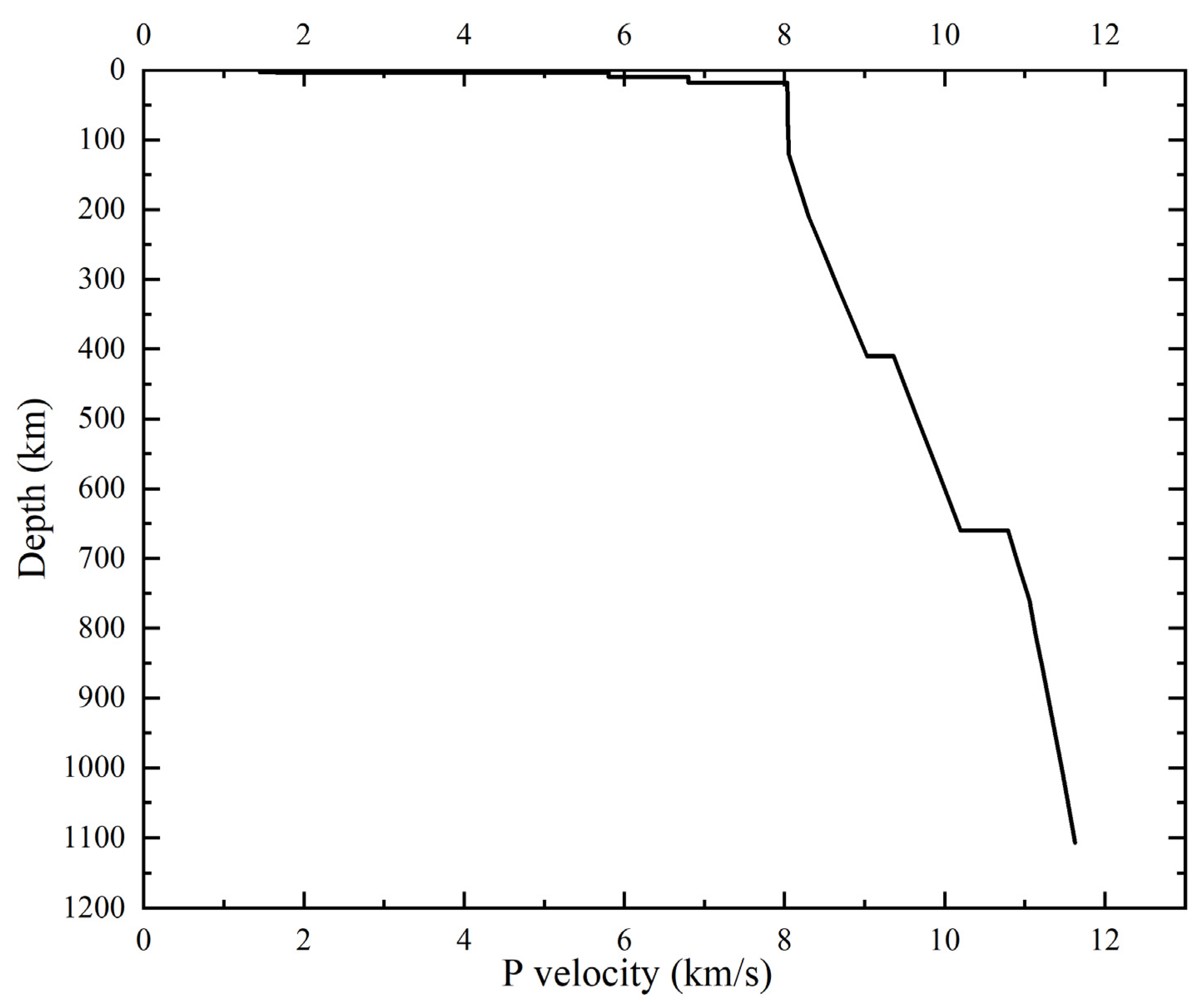
- Calculating travel time and travel time residuals in 1-D and 3-D crust models, respectively. In this paper, the average depth of the Moho surface of 30 km is taken as the thickness of the crust, the crust contains upper, middle and lower layers. The calculation formula is as follows:where δTcrust represents the relative travel time residuals in the crust, T indicates the travel time in the crust, h indicates the thickness of each layer in the crust, θ represents the incident angle of rays at each interface and V denotes the velocity in each layer. The 3-D and 1-D subscripts indicate 3D crust model and 1-D model, respectively.
- (3)
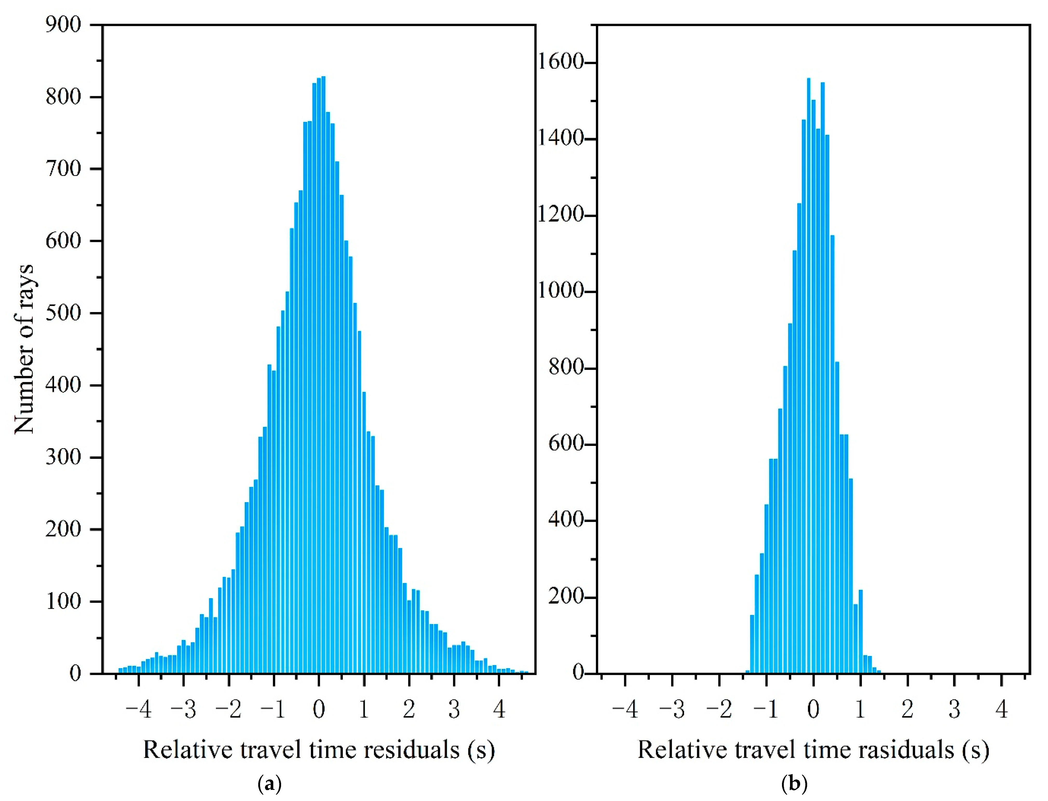
- The real data used in the tomographic calculation are the measured travel time minus the theoretical travel time and then minus the travel time residuals in the crust. The expression of the formula is as follows:where t represents the relative travel time residuals, Tobs indicates the measured travel time and Tcal the theoretical travel time.
2.3. Methods
3. Resolution Tests and Results
3.1. Resolution Tests
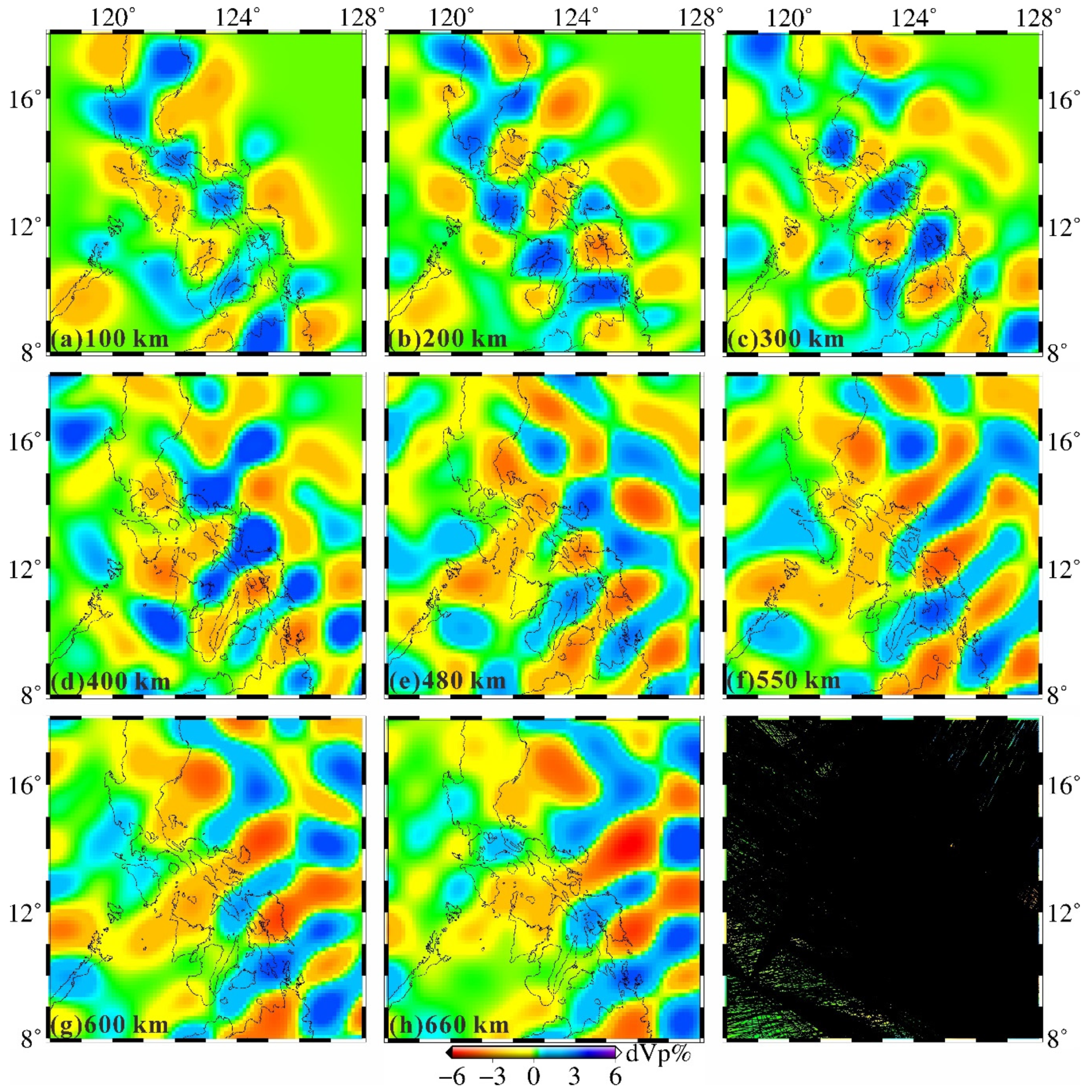
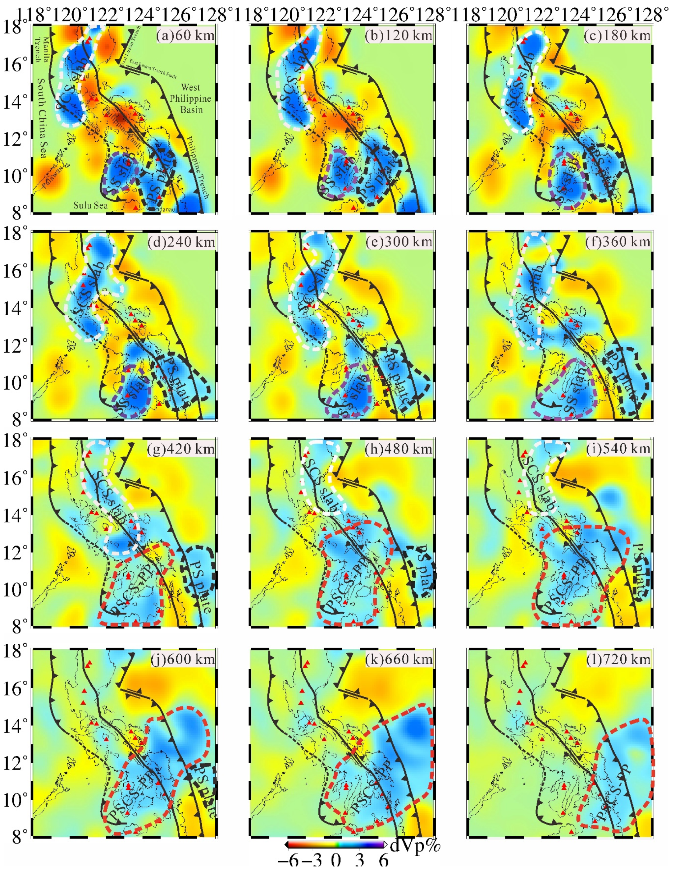
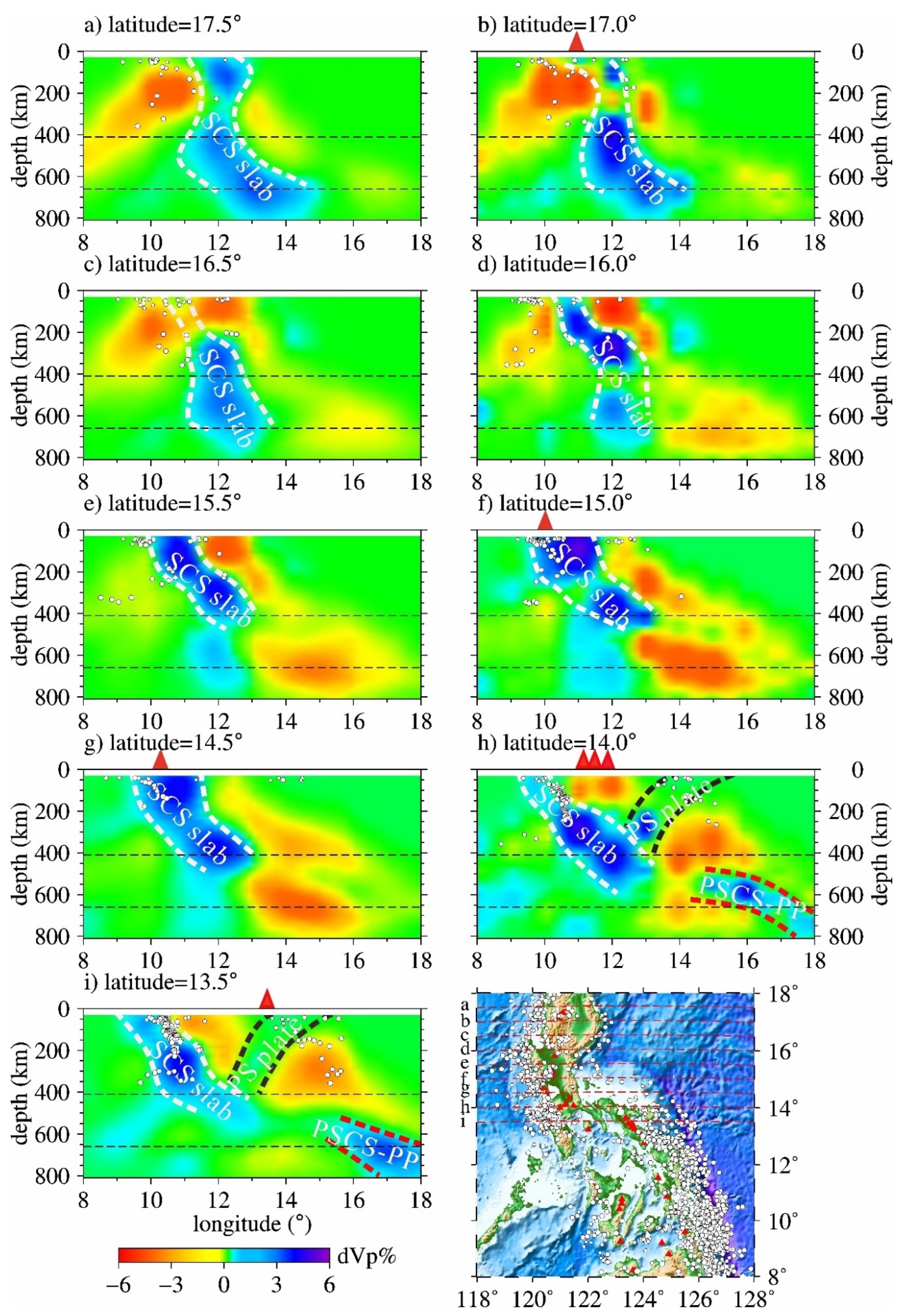
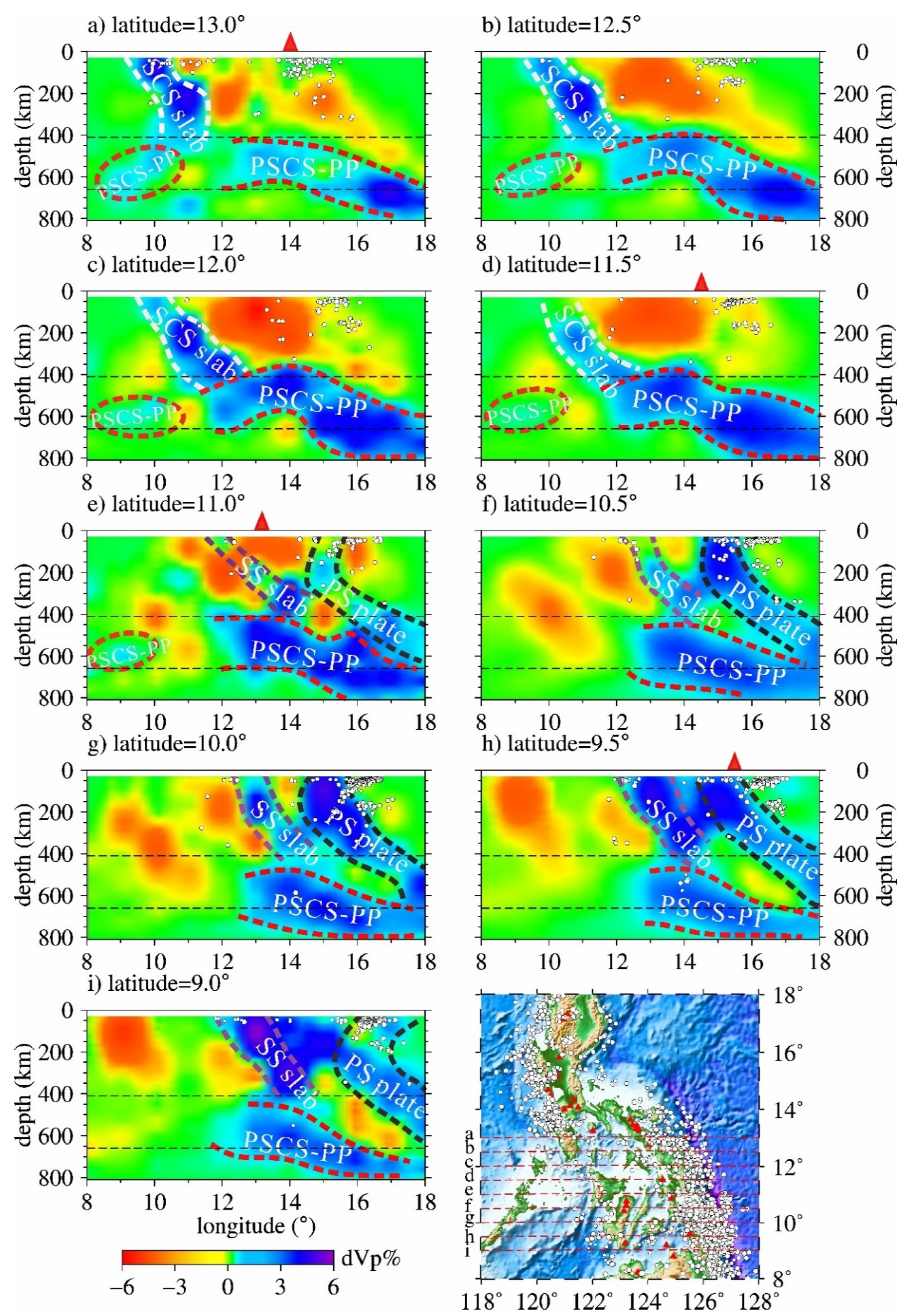
3.2. Results
4. Discussion
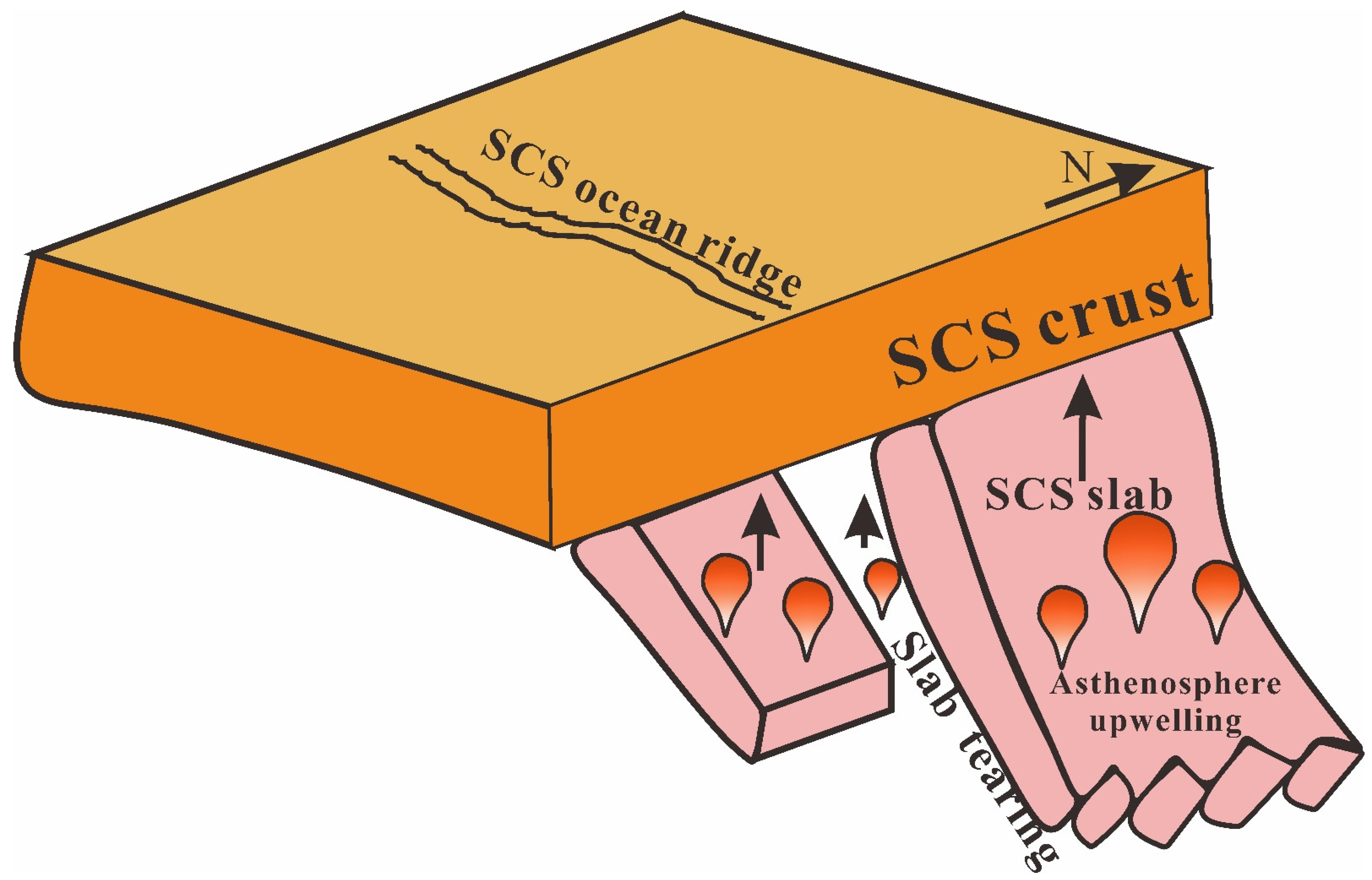
4.1. Subduction of South China Sea
4.2. Subduction of Proto-South China Sea
4.3. Subduction of Philippine Sea and Sulu Sea
5. Conclusions
Author Contributions
Funding
Data Availability Statement
Acknowledgments
Conflicts of Interest
References
- Bautista, B.C.; Bautista, M.L.P.; Oike, K.; Wu, F.T.; Punongbayan, R.S. A new insight on the geometry of subducting slabs in northern Luzon, Philippines. Tectonophysics 2001, 339, 279–310. [Google Scholar] [CrossRef]
- Aurelio, M.A. Shear partitioning in the Philippines: Constraints from Philippine Fault and global positioning system data. Island Arc 2008, 9, 584–597. [Google Scholar] [CrossRef]
- Taylor, B.; Hayes, D.E. Origin and History of the South China Sea Basin; American Geophysical Union (AGU): Washington, DC, USA, 1983; pp. 23–56. [Google Scholar]
- Tapponnier, P.; Lacassin, R.; Leloup, P.H.; Schärer, U.; Dalai, Z.; Haiwei, W.; Xiaohan, L.; Shaocheng, J.; Lianshang, Z.; Jiayou, Z. The Ailao Shan/Red River metamorphic belt: Tertiary left-lateral shear between Indochina and South China. Nat. Cell Biol. 1990, 343, 431–437. [Google Scholar] [CrossRef]
- Morley, C.; Morley, C. A tectonic model for the Tertiary evolution of strike–slip faults and rift basins in SE Asia. Tectonophysics 2002, 347, 189–215. [Google Scholar] [CrossRef]
- Chung, S.-L.; Sun, S.-S.; Tu, K.; Chen, C.-H.; Lee, C.-Y. Late Cenozoic basaltic volcanism around the Taiwan Strait, SE China Sea: Product of lithosphere1asthenosphere interaction during continental extension. Chem. Geol. 1994, 112, 1–20. [Google Scholar] [CrossRef]
- Tang, Q.; Chan, Z. Crust and upper mantle structure and its tectonic implication in the SCS and adjacent regions. J. Asian Earth Sci. 2013, 62, 510–525. [Google Scholar] [CrossRef]
- Sibuet, J.-C.; Yeh, Y.-C.; Lee, C.-S. Geodynamics of the South China Sea. Tectonophysics 2016, 692, 98–119. [Google Scholar] [CrossRef] [Green Version]
- Huang, C.-Y.; Wang, P.; Yu, M.; You, C.-F.; Liu, C.-S.; Zhao, X.; Shao, L.; Zhong, G.; Yumul, G.P. Potential role of strike-slip faults in opening up the South China Sea. Natl. Sci. Rev. 2019, 6, 891–901. [Google Scholar] [CrossRef]
- Hall, R. Cenozoic geological and plate tectonic evolution of SE Asia and the SW Pacific: Computer-based reconstructions, model and animations. J. Asian Earth Sci. 2002, 20, 353–431. [Google Scholar] [CrossRef]
- Fan, J.-K.; Wu, S.-G.; Spence, G. Tomographic evidence for a slab tear induced by fossil ridge subduction at Manila Trench, South China Sea. Int. Geol. Rev. 2014, 57, 998–1013. [Google Scholar] [CrossRef]
- Fan, J.; Zhao, D.; Dong, D.; Zhang, G. P-wave tomography of subduction zones around the central Philippines and its geo-dynamic implications. J. Asian Earth Sci. 2017, 146, 76–89. [Google Scholar] [CrossRef]
- Fan, J.; Zhao, D. Evolution of the Southern Segment of the Philippine Trench: Constraints from Seismic Tomography. Geochem. Geophys. Geosyst. 2018, 19, 4612–4627. [Google Scholar] [CrossRef]
- Tan, H.; Wang, Z. Seismic velocity imaging and tectonic characteristic of the bidirectional subducting slabs under Philipppine Archipelago. Chin. J. Geophys. 2018, 61, 4887–4990. (In Chinese) [Google Scholar]
- Tan, H.; Wang, Z. The Vp and Vs tomography of Taiwan, China-Philippine Archipelago and its tectonic implications. Earthq. Res. China 2018, 34, 473–483. [Google Scholar]
- Fan, J.; Zhao, D. P-wave anisotropic tomography of the central and southern Philippines. Phys. Earth Planet. Inter. 2019, 286, 154–164. [Google Scholar] [CrossRef]
- Rangin, C.; Spakman, W.; Pubellier, M.; Bijwaard, H. Tomographic and geological constraints on subduction along the eastern Sundaland continental margin (South-East Asia). Bull. Soc. Geol. Fr. 1999, 170, 775–788. [Google Scholar]
- Clift, P.; Lee, G.H.; Duc, N.A.; Barckhausen, U.; Van Long, H.; Zhen, S. Seismic reflection evidence for a Dangerous Grounds miniplate: No extrusion origin for the South China Sea. Tectonics 2008, 27, TC3008. [Google Scholar] [CrossRef]
- Hall, R.; Spakman, W. Mantle structure and tectonic history of SE Asia. Tectonophysics 2015, 658, 14–45. [Google Scholar] [CrossRef] [Green Version]
- Wu, J.; Suppe, J. Proto-South China Sea Plate Tectonics Using Subducted Slab Constraints from Tomography. J. Earth Sci. 2018, 29, 1304–1318. [Google Scholar] [CrossRef] [Green Version]
- Shi, H.; Li, T.; Zhang, R.; Zhang, G.; Yang, H. Imaging of the Upper Mantle Beneath Southeast Asia: Constrained by Teleseismic P-wave Tomography. Remote Sens. 2020, 12, 2975. [Google Scholar] [CrossRef]
- Lin, Y.; Colli, L.; Wu, J.; Schuberth, B.S.A. Where Are the Proto-South China Sea Slabs? SE Asian Plate Tectonics and Mantle Flow History From Global Mantle Convection Modeling. J. Geophys. Res. Solid Earth 2020, 125, 125. [Google Scholar] [CrossRef]
- International Seismological Centre (2021), On-line Bulletin. Available online: http://www.isc.ac.uk/iscbulletin/search/ (accessed on 1 May 2021).
- Zhao, D.; Hasegawa, A.; Kanamori, H. Deep structure of Japan subduction zone as derived from local, regional, and teleseismic events. J. Geophys. Res. Space Phys. 1994, 99, 22313–22329. [Google Scholar] [CrossRef]
- Li, Z.; Roecker, S.; Kim, K.; Xu, Y.; Hao, T. Moho depth variations in the Taiwan orogen from joint inversion of seismic arri-val time and Bouguer gravity data. Tectonophysics 2014, 632, 151–159. [Google Scholar] [CrossRef]
- Li, X.; Hao, T.; Li, Z. Upper mantle structure and geodynamics of the Sumatra subduction zone from 3-D teleseismic P-wave tomography. J. Asian Earth Sci. 2018, 161, 25–34. [Google Scholar] [CrossRef]
- Obayashi, M.; Suetsugu, D.; Fukao, Y. PP-Pdifferential travel time measurement with crustal correction. Geophys. J. Int. 2004, 157, 1152–1162. [Google Scholar] [CrossRef] [Green Version]
- Tian, Y.; Hung, S.-H.; Nolet, G.; Montelli, R.; Dahlen, F.A. Dynamic ray tracing and travel time corrections for global seismic tomography. J. Comput. Phys. 2007, 226, 672–687. [Google Scholar] [CrossRef]
- Jiang, G.M.; Zhao, D.P.; Zhang, G.B. Crustal correction in teleseismic tomography and its application. Chin. J. Geophys. 2009, 52, 1508–1514. [Google Scholar]
- Kennett, B.L.N.; Engdahl, E.R.; Buland, R. Constraints on seismic velocities in the Earth from travel times. Geophys. J. Int. 1995, 122, 108–124. [Google Scholar] [CrossRef]
- Laske, G.; Masters, G.; Ma, Z.; Pasyanos, M. Update on CRUST1. 0-A 1-degree global model of Earth’s crust. EGU Gen. Assem. Conf. Abstr. 2013, 15, 2658. [Google Scholar]
- Rawlinson, N.; De Kool, M.; Sambridge, M. Seismic wavefront tracking in 3D heterogeneous media: Applications with multi-ple data classes. Explor. Geophys. 2006, 37, 322–330. [Google Scholar] [CrossRef]
- Rawlinson, N.; Kennett, B.L.N. Teleseismic tomography of the upper beneath the southern Lachlan Orogen, Australia. Phys. Earth Planet. Int. 2008, 167, 84–97. [Google Scholar] [CrossRef]
- Kennett, B.N.L.; Sambridge, M.; Williamson, P.R. Subspace methods for large scale inverse problems involving multiple pa-rameter classes Geophys. J. Int. 1988, 94, 237–247. [Google Scholar]
- Sethian, J.A.; Popovici, A.M. 3-D traveltime computation using the fast marching method. Geophysics 1999, 64, 516–523. [Google Scholar] [CrossRef]
- Macpherson, K.A.; Hidayat, D.; Goh, S.H. Receiver function structure beneath four seismic stations in the Sumatra region. J. Asian Earth Sci. 2012, 46, 161–176. [Google Scholar] [CrossRef]
- Dickson, W.R.; Snyder, W.S. Deometry of subducted slabs related to San Andreas transform. Geology 1979, 87, 609–627. [Google Scholar] [CrossRef]
- Thorkelson, D.J.; Taylor, R.P. Cordilleran slab window. Geology 1989, 17, 833–836. [Google Scholar] [CrossRef]
- Richards, S.; Lister, G.; Kennett, B. A slab in depth: Three-dimensional geometry and evolution of the Indo-Australian plate. Geochem. Geophys. Geosyst. 2007, 8, Q12003. [Google Scholar] [CrossRef] [Green Version]
- Chen, Y.; Li, W.; Yuan, X.; Badal, J.; Teng, J. Tearing of the Indian lithospheric slab beneath southern Tibet revealed by SKS-wave splitting measurements. Earth Planet. Sci. Lett. 2015, 413, 13–24. [Google Scholar] [CrossRef]
- Rao, C.V.D.; Santosh, M.; Zhang, S.-H. Neoproterozoic massif-type anorthosites and related magmatic suites from the East-ern Ghats Belt, India: Implications for slab window magmatism at the terminal stage of collisional orogeny. Precambrian Res. 2014, 240, 60–78. [Google Scholar] [CrossRef]
- Syuhada, S.; Hananto, N.D.; Abdullah, C.I.; Puspito, N.T.; Anggono, T.; Febriani, F.; Soedjatmiko, B. Lithospheric mantle anisotropy from local events beneath the Sunda–Banda arc transition and its geodynamic implications. Acta Geophys. 2020, 68, 1565–1593. [Google Scholar] [CrossRef]
- He, Q.Y.; Hao, T.F.; Xing, J.; Li, X.B.; Li, C.W. Study of intracrustal density structure in the Sumatra subduction zone region. J. Geophys. 2021, 64, 569–581. [Google Scholar]
- Tang, Q.Q.; Zhan, W.H.; Li, J.; Feng, Y.C.; Yao, Y.T.; Sun, J.; Li, Y.H. Plate window tectonics reflected by volcanic activity on the eastern margin of the South China Sea. Mar. Geol. Quat. Geol. 2017, 37, 119–126. [Google Scholar]
- Peacock, S.M.; Van Keken, P.E.; Holloway, S.D.; Hacker, B.R.; Abers, G.A.; Fergason, R.L. Thermal structure of the Costa Rica—Nicaragua subduction zone. Phys. Earth Planet. Inter. 2005, 149, 187–200. [Google Scholar] [CrossRef]
- Brandes, C.; Winsemann, J. From incipient island arc to doubly-vergent orogen: A review of geodynamic models and sedi-mentary basin-fills of southern Central America. Island Arc 2018, 27, e12255. [Google Scholar] [CrossRef]
- Barckhausen, U.; Engels, M.; Franke, D.; Ladage, S.; Pubellier, M. Evolution of the South China Sea: Revised ages for breakup and seafloor spreading. Mar. Pet. Geol. 2014, 58, 599–611. [Google Scholar] [CrossRef]
- Ru, K.; John, D. Pigott Episodic Rifting and Subsidence in the South China Sea: ERRATUM. AAPG Bull. 1987, 71, 119. [Google Scholar]
- Yao, B.; Zeng, W.; Hayes, D.E.; Spangler, S. The Geological Memoir of South China Sea Surveyed Jointly by China and USA; China University of Geosciences: Wuhan, China, 1994. [Google Scholar]
- Zahirovic, S.; Seton, M.; Müller, R.D. The Cretaceous and Cenozoic tectonic evolution of Southeast Asia. Solid Earth 2014, 5, 227–273. [Google Scholar] [CrossRef] [Green Version]
- Zhou, D.; Sun, Z. Plate evolution in the Pacific domain since Late Mesozoic and its inspiration to tectonic research of East Asia margin. J. Trop. Oceanogr. 2017, 36, 1–19. [Google Scholar]
- Yumul, G.P., Jr.; Dimalanta, C.B.; Tamayo, R.A., Jr.; Maury, R.C. Collision, subduction and accretion events in the Phil-ippines: A synthesis. Isl. Arc 2003, 12, 77–91. [Google Scholar] [CrossRef]
- Fischer, M.C.S. Hutchison 1989. Geological Evolution of South-East Asia. Oxford Monographs on Geology and Geophysics no. 13. xv + 368 pp. Oxford: Clarendon Press. Price £65.00 (hard covers). 0 19 854439 1. Geol. Mag. 1990, 127, 185. [Google Scholar] [CrossRef]
- Zhao, S.; Li, X.J.; Yao, Y.J.; Xie, X.N.; Xiao, S.Y.; He, X.; Deng, Y.T.; Shi, M.L.; Zhou, M. Orogenic events in southern South China Sea and their relationship with the subduction of the Proto South China Sea. Mar. Geol. Quat. Geol. 2019, 39, 147–162. [Google Scholar]
- Bondár, I.; Storchak, D.A. Improved location procedures at the International Seismological Centre. Geophys. J. Int. 2011, 186, 1220–1244. [Google Scholar] [CrossRef] [Green Version]
- Willemann, R.J.; Storchak, D.A. Data Collection at the International Seismological Centre. Seis. Res. Lett. 2001, 72, 440–453. [Google Scholar] [CrossRef] [Green Version]
- Wessel, P.; Smith, W.H.F. New, improved version of generic mapping tools released. Eos Trans. Am. Geophys. Union 1998, 79, 579. [Google Scholar] [CrossRef]


Publisher’s Note: MDPI stays neutral with regard to jurisdictional claims in published maps and institutional affiliations. |
© 2021 by the authors. Licensee MDPI, Basel, Switzerland. This article is an open access article distributed under the terms and conditions of the Creative Commons Attribution (CC BY) license (https://creativecommons.org/licenses/by/4.0/).
Share and Cite
Shi, H.; Li, T.; Sun, R.; Zhang, G.; Zhang, R.; Kang, X. Insights from the P Wave Travel Time Tomography in the Upper Mantle Beneath the Central Philippines. Remote Sens. 2021, 13, 2449. https://0-doi-org.brum.beds.ac.uk/10.3390/rs13132449
Shi H, Li T, Sun R, Zhang G, Zhang R, Kang X. Insights from the P Wave Travel Time Tomography in the Upper Mantle Beneath the Central Philippines. Remote Sensing. 2021; 13(13):2449. https://0-doi-org.brum.beds.ac.uk/10.3390/rs13132449
Chicago/Turabian StyleShi, Huiyan, Tonglin Li, Rui Sun, Gongbo Zhang, Rongzhe Zhang, and Xinze Kang. 2021. "Insights from the P Wave Travel Time Tomography in the Upper Mantle Beneath the Central Philippines" Remote Sensing 13, no. 13: 2449. https://0-doi-org.brum.beds.ac.uk/10.3390/rs13132449