The Dynamical Structure of a Warm Core Ring as Inferred from Glider Observations and Along-Track Altimetry

Abstract

This study investigates the vertical structure of the dynamical properties of a warm-core ring in the Gulf of Mexico (Loop Current ring) using glider observations. We introduce a new method to correct the glider’s along-track coordinate, which is, in general, biased by the unsteady relative movements of the glider and the eddy, yielding large errors on horizontal derivatives. Here, we take advantage of the synopticity of satellite along-track altimetry to apply corrections on the glider’s position by matching in situ steric height with satellite-measured sea surface height. This relocation method allows recovering the eddy’s azimuthal symmetry, precisely estimating the rotation axis position, and computing reliable horizontal derivatives. It is shown to be particularly appropriate to compute the eddy’s cyclo-geostrophic velocity, relative vorticity, and shear strain, which are otherwise out of reach when using the glider’s raw traveled distance as a horizontal coordinate. The Ertel potential vorticity (PV) structure of the warm core ring is studied in details, and we show that the PV anomaly is entirely controlled by vortex stretching. Sign reversal of the PV gradient across the water column suggests that the ring might be baroclinically unstable. The PV gradient is also largely controlled by gradients of the vortex stretching term. We also show that the ring’s total energy partition is strongly skewed, with available potential energy being 3 times larger than kinetic energy. The possible impact of this energy partition on the Loop Current rings longevity is also discussed.

1. Introduction

During the past two decades, gliders (autonomous underwater vehicles) have become widespread, reliable, flexible, and cost-effective measurement platforms [1,2,3,4]. They were shown to be appropriate for measuring most oceanic features and processes on a variety of time and space scales, including high-frequency internal waves [5], intense surface boundary currents [6], mesoscale and submesoscale eddies [7,8,9,10], fine-scale thermohaline stirring [11], or turbulent mixing [12].

Because gliders only use buoyancy and lift to move, they are slow vehicles, and the subsequent lack of synopticity is their Achilles’ heel. The limits of glider measurements were extensively discussed by the authors of [3], who showed that their slow speed can result in the contamination of spatial structures by high frequency temporal variability, such as internal waves. They suggested that low-pass filtering scales smaller than O[30 km] was necessary to avoid this contamination when representing the measured variables in isobaric coordinates, as is necessary when computing geostrophic velocity and other derived variables. Recently, the authors of [9] showed that gliders slowness could also produce significant bias in geostrophic velocity estimates, even when applying an appropriate low-pass filter, when sampling quickly evolving structures such as fast-drifting eddies. As a glider crosses an eddy traveling in the opposite direction, the radius of the eddy is underestimated, while it is overestimated in the case of a glider crossing an eddy drifting in the same direction. As the horizontal coordinate available to compute density gradients is the glider’s traveled distance, this results in an overestimation or underestimation of geostrophic velocity. This error was shown to sometimes reach nearly $50\%$ in the case of Loop Current rings (LCR) in the Gulf of Mexico (GoM) [9].

LCRs are large anticyclonic eddies detaching from the Loop Current and transporting warm and salty subtropical underwater from the Caribbean to the western GoM [13,14,15] (Figure 1). They are close cousins of other well-known warm-core rings detaching from the Gulf Stream [16,17], Kuroshio [18,19], North Brazil current [20], and the Agulhas current [21,22]. Warm-core rings generally consist of a core of nearly homogeneous and anomalously high temperature (also known as the thermostad) surrounded by an annulus of high azimuthal velocity at their periphery [23]. Because they are long-lived, coherent, and carry large amounts of heat, warm-core rings can impact oceanic basins thermohaline properties [22,24], and understanding their thermohaline and dynamical properties is crucial.

While the vertical thermohaline structure of Loop Current rings was described in detail [9,10,11,14,25], little is known of their dynamical properties, such as their Ertel’s potential vorticity (PV) structure or the distribution and partition of energy density in their cores. However, the longevity of LCRs and their ability to transport tracers over long distances largely depend on their coherence and their stability properties, which depend on the relative importance of strain and vorticity, and on their PV distribution, respectively.

The present work is a follow-up of the work in [9] on the vertical structure of a Loop Current ring using glider observations. Here, we focus on the dynamical properties of a recently formed LCR, and pay particular attention to its PV structure. Our analysis is based on the use of a new method based on along-track altimetry to compensate for the lack of synopticity of the glider measurements across a fast-drifting eddy. The glider survey and the altimetry data are described in Section 2, while the correction method is presented in detail in Section 3. In Section 4, we describe the vertical structure of the LCR in terms of velocity, relative vorticity, shear strain, Okubo–Weiss parameter (OW), and PV. All terms contributing to the PV anomaly (PVA) are described in detail, and the distribution of the available potential energy density (APED) and kinetic energy density (KED) is also presented. The efficiency and relevancy of the correction method, as well as the vertical dynamical structure of the LCR are discussed in Section 5.

2. Data

2.1. The Glider Survey

In situ data were collected across a recently detached LCR in the central GoM between 05/08 and 03/09/2016, using a Kongsberg Sea Glider. The vehicle oscillated between the surface and a maximum depth of 1000 m, at mean horizontal and vertical speeds of 0.15 $\mathrm{m}{\mathrm{s}}^{-1}$. It was equipped with an unpumped CTD probe (Seabird CTsail) with a sampling frequency of 0.15 Hz, resulting in effective average horizontal and vertical resolutions of 2000 m and 2 m, respectively. However, large variability of the flow speed as the glider crossed the eddy resulted in large variability of the absolute horizontal speed, and thus of the horizontal resolution (500 m to 7 km). The glider’s trajectory is shown in Figure 2a along with successive edge-contours of the LCR inferred from gridded satellite altimetry. The glider crossed the LCR through its center, and its trajectory was essentially orthogonal to sea surface height (SSH) contours. A detailed description of the glider survey is available in [9]. As the glider’s exact underwater position cannot be directly measured, we approximate each dive as a vertical profile located at the median position between diving and surfacing.

2.2. Satellite Altimetry

All altimetry products used in this study are AVISO absolute dynamic topography. The relocation method relies on individual along-track satellite observations, while eddy detection is performed using a multi-satellite merged gridded product. The along-track observations offer a synoptic view of SSH along a given trajectory (full-eddy crossing in about one minute), with high resolution (7 km), while the gridded SSH fields offer a coarser (0.25${}^{\circ }$ resolution), but 2-dimensional view, that allow us to approximately detect the eddy’s edge and center.

We used the eddy detection algorithm in [24], which defines the edge of the eddy as the maximum circulation contour, which is the ADT contour along which the path integral of geostrophic velocity is maximum. The center of the eddy is then simply defined as the center of mass of this contour. Although AVISO provides filtered along-track observations, we used the original unfiltered ADT data, that we low-pass filtered using the local first Rossby radius as a cut-off wavelength (45 km [26]).

3. Methods

3.1. The Relocation Method

LCRs drift at an average speed of 0.05 $\mathrm{m}{\mathrm{s}}^{-1}$, but can eventually reach up to 0.1 $\mathrm{m}{\mathrm{s}}^{-1}$ [9,27]. The slow speed of the gliders, along with the relatively quick evolution of LCRs can result in synopticity issues. In particular, the use of the glider’s traveled distance as the reference horizontal coordinate was shown to yield significant errors when computing gradients [9]. For instance, if a glider is navigating across an eddy in the opposite direction of the eddy’s drift, glider-inferred distances will be shortened and the gradients will be overestimated, while a glider navigating in the same direction as the eddy’s drift will induce an overestimation of distances and an underestimation of gradients [9]. Variability of the eddy’s drift speed, along with the variability of the glider’s horizontal speed as it navigates through more or less intense currents, result in a chaotic horizontal coordinate when using the glider’s traveled distance as a reference. The authors of [9] proposed a correction factor for glider-derived geostrophic velocity $U_g$ computed for an eddy drifting at a speed $U_e$ as $C_f=U_g/(U_g-U_e)$. They estimated that, for the LCR discussed in the present paper, the correction factor varies from 0.5 to 1.4, yielding an error in the geostrophic velocity magnitude ranging between −50% and +40%.

Reliable computation of the geostrophic and cyclogeostrophic velocities, as well as relative vorticity and strain, or any gradient-based variable, should ideally be performed in a frame of reference drifting with the eddy, or the transect should be performed quasi-instantaneously, which is obviously impossible.

On the other hand, satellites, which measure Sea Surface Height (SSH), are able to cross an LCR in a matter of one minute, and along-track SSH profiles provide a fully synoptic description. In this work, we take advantage of the synopticity of the surface observations by satellite altimeters to relocate the glider observations in a new frame of reference. Figure 2b shows a selected series of satellite tracks that crossed the LCR during its drift in the central and western GoM, and Figure 2c shows the corresponding along-track SSH profiles across the LCR.

To relocate the glider observations in a synoptic frame of reference, first we select one satellite track that is most closely parallel to the glider transect and crosses the eddy through its center at the approximate same time as the glider. Then, we compute the in situ steric height referenced to 1000 dbar for each glider dive, under the assumption that this pressure level can be considered as the level of no motion (flat geopotential). The steric height ${\eta }_g$ is defined as

$${\eta }_g={\rho }_0{\int }_{-H}^0(\rho {\left(z\right)}^{-1}-{\rho }_0^{-1})dz,$$

(1)

where $\rho$ is a density profile obtained during a glider dive, and ${\rho }_0$ is an arbitrary reference density. We then search, for each glider’s dive, the data point in the along-track altimetry that most closely matches the glider’s steric height, and relocate the glider dive to that point (Figure 3b).

As both satellite altimetry and in situ steric height are relative measurements which require a level of reference, it is necessary to define a common reference. To do so, we define the zero SSH level as the mode of the SSH distribution in the GoM. For altimeter-derived SSH (${\eta }_a$), the mode of the distribution is computed using all available altimetry data in the 2014–2018 period. For the glider-derived SSH (steric height), we use the steric height of all available ARGO profiles. The ARGO dataset consists of 3995 validated profiles acquired in the GoM, sampling down to depths greater than 1000 m, with a minimum vertical resolution of 10 m. The dataset, as well as the probability density functions of satellite SSH and in situ steric height are fully described in [9]. To validate the comparability of ADT and in situ 0–1000 dbar steric height, we compared the steric height of all ARGO profiles with the local ADT from the gridded product. Despite the coarse resolution of the grid (0.25${}^{\circ }$), and the time aliasing issues of gridded ADT (related to the interpolation of along-track data in both time and space), the correlation between the closest grid-point ADT value and in situ steric height is high (coefficient of determination of 0.93). To compensate for time-aliasing issues and the lack of synopticity of gridded ADT from our validation, we also computed the closest-matching ADT value in a radius of 50 km from the in situ profile. In that case, the correlation becomes excellent, with a coefficient of determination of 0.99, suggesting that the 1000–0 dbar steric height is a goof proxy for SSH, and that the errors are mostly caused by interpolation-related spatial uncertainties in the gridded ADT product, that do not occur in along-track observations.

Figure 3 compares a cross-eddy steric height profile computed from glider data, an SSH profile from a gridded altimeter product, estimated along the glider track, and the selected along-track altimeter SSH profile.

Comparing the along track satellite SSH and the glider’s steric height (Figure 3a) reveals the spatial bias induced by the slow and irregular sampling of the glider. While the instantaneous SSH profile of the eddy, as observed by along-track altimetry, closely matches a Gaussian distribution, the glider’s representation tends to flatten the SSH distribution near the center of the eddy, and to overestimate the eddy’s size.

Note that although the glider’s track crossed the eddy’s center (as estimated from the gridded altimetry product), its trajectory is not exactly straight and not always strictly parallel to the SSH gradient. As the along-track thermohaline gradients are the only available information, the geostrophic currents computed from the raw (uncorrected) glider observations only provide the across-track velocity component. If the glider’s track is not strictly parallel to the thermohaline gradient, then there exists an along-track velocity component, which the glider is not able to measure, and the computed velocity is biased. However, here, as we relocate the glider’s observations along a straight satellite track passing through the eddy’s center, and is by definition essentially parallel to the SSH gradients, this bias is eliminated.

Hereafter, all fields are computed by relocating the glider’s dives to the closest matching SSH point in the along-track SSH profile shown in Figure 3a.

3.2. Validation

To validate the relocation methods, we simulated four different glider surveys across an idealized stable and circular anticyclonic eddy drifting on the $\beta$-plane. The eddy’s SSH signature is chosen to be a generalized Gaussian function:

$$\begin{array}{c}\hfill {\eta }_e\left(r\right)={\eta }_0{e}^{-\frac{{\left|r\right|}^3}{R^3}},\end{array}$$

(2)

where ${\eta }_e$ is the eddy’s SSH, ${\eta }_0$ is the maximum SSH at the eddy’s centre, r is the radial coordinate, and R is the eddy’s radius. The vertical structure of the eddy was chosen to represent a typical warm-core ring, with vertically homogeneous temperature and salinity anomalies in the core (Figure 4). Note that the particular structure of the eddy has little importance, as the purpose is only to validate a method that should be indifferent to the choice of the eddy’s vertical structure.

The mean virtual glider speed is set to 0.15 m s${}^{-1}$, with a random fluctuation ranging between −0.075 m s${}^{-1}$ and +0.075 m s${}^{-1}$. The eddy is drifting south-west at a speed of 0.07 m s${}^{-1}$. The first two experiments consist in an ideal straight-line sampling along the exact trajectory of the eddy’s center. One is performed in the opposite direction to the eddy’s drift (hereafter updrift survey; Figure 5a), and the other in the direction of the eddy’s drift (hereafter downdrift survey; Figure 5b)). We also simulate a manually piloted glider survey, starting at about 100 km south of the eddy’s initial position, and aiming towards the eddy’s center as estimated from incomplete SSH information (a random uncertainty of 50 km on the eddy’s location was added and the maps are only updated every 3 days) (hereafter typical survey; Figure 5c). Finally, a second manually piloted experiment is simulated, using the same virtual piloting conditions as the typical survey, but using a spiraling approach strategy (hereafter spiral survey; Figure 5d).

Figure 6a compares the different SSH profiles computed as the local steric height along the simulated glider surveys for the four experiments, along with the true synoptic SSH profile (instantaneous measurement). The Radial distance is computed as the distance traveled by the glider, centred at the location of the SSH maximum. As expected, the updrift survey yields an underestimation of the eddy’s size, while the downdrift survey yields an overestimation. The typical survey, whose sampling direction is essentially updrift slightly underestimate the eddy’s size, but, most importantly, the Gaussian eddy’s shape appears to be irregular. The spiraling survey is an extreme example of the bias introduced by the sampling strategy: the eddy appears over three times larger than it really is and some random variability is also evident. The resulting surface geostrophic velocity is shown on Figure 6b. As expected from the bias in the horizontal along-track coordinate, the updrift and downdrift surveys exhibit smaller and larger velocity maxima, respectively, along with artificial variability associated with the random sampling speed. In the case of the typical survey, with an irregular trajectory and velocity of the glider, the velocity maximum is underestimated on one side of the eddy and overestimated on the other, and spurious small scale variability is added. The spiral survey clearly underestimates the velocity and the maxima are unidentifiable because of the high noise level and underestimated gradients.

Virtual observations of all four simulated surveys were corrected using the relocation method. Comparison of uncorrected and corrected azimuthal velocity sections are shown in Figure 7. The difference between the corrected and uncorrected velocity fields is also shown in the right-hand side panels. In all cases, the method, which relocates each vertical profile into a synoptic frame of reference precisely recovers the eddy’s true vertical structure.

3.3. Theoretical Framework

In this work, the Ertel’s Potential Vorticity (PV) structure of the LCR is described in detail. Following the work in [28], PV is defined as

$$q=\frac{1}{\sigma }\mathit{\omega }·\mathbf{\nabla }\sigma ,$$

(3)

where q is PV, $\sigma$ is potential density, and $\mathit{\omega }$ is the absolute vorticity vector. Using the assumptions of a purely azimuthal flow, and of azimuthal symmetry of the eddy, and expressing the vertical density gradient in terms of the squared Brunt–Väisälä frequency ($N^2=-g{\partial }_z\sigma /\sigma$, where g is the gravity acceleration), PV can be rewritten as

$$q=\frac{1}{g}(f+\zeta )N^2-\frac{1}{\sigma }{\partial }_z{u}_{\varphi }{\partial }_r\sigma ,$$

(4)

where f is the Coriolis frequency, r is the radial coordinate, and $u_{\varphi }$ is the azimuthal velocity. $u_{\varphi }$ is computed using the gradient wind balance (cyclogeostrophy), following the work in [29]:

$$u_{\varphi }(r,z)=\frac{2u_{\varphi }^g(r,z)}{1\pm \sqrt{1+4u_{\varphi }^g(r,z)/fr}},$$

(5)

where $u_{\varphi }^g(r,z)$ is the geostrophic velocity, defined as

$$u_{\varphi }^g(r,z)=u_{\varphi }^g(r,0)-\frac{g}{f{\rho }_0}{\int }_z^0{\partial }_r\rho (r,\tilde{z})d\tilde{z}.$$

(6)

where ${\rho }_0$ is a mean density, $\rho (r,z)$ is in situ density, $\tilde{z}$ is an integration variable, and the geostrophic velocity at the surface is computed from the along-track altimetry profile as

$$u_{\varphi }^g(r,0)=\frac{g}{f}{\partial }_r{\eta }_a$$

(7)

Using the azimuthal symmetry assumption, relative vorticity $\zeta$ is defined as

$$\zeta =\frac{1}{r}{\partial }_r\left(r{u}_{\varphi }\right),$$

(8)

Although PV is a scalar, we will refer to the two terms of Equation (4) as the vertical (first term), and baroclinic (second term) PV components.

We will also estimate and discuss the PV anomaly (PVA), which is the difference between PV and the ambient PV at rest along isopycnal surfaces:

$$\begin{array}{ccc}\hfill q^{*}\left(\sigma \right)& =& q\left(\sigma \right)-\frac{f}{g}{\overline{N}}^2\left(\sigma \right).\hfill \end{array}$$

(9)

In this work, the reference PV is computed on an f-plane using the Coriolis frequency at 25.5${}^{\circ }$N, and the mean stratification profile was computed using GoM’s ARGO float dataset described in Section 3.1. The float profiles were selected to be representative of Gulf Common water (GCW), which we define as the profiles whose steric height lies within half a standard deviation from the mode of the GoM’s SSH distribution.

By decomposing the squared Brunt–Väisälä frequency into a mean and a perturbation part ($N^2=\overline{N^2}+N_a^2$), we can decompose PVA into four terms [10]:

$$\begin{array}{ccc}\hfill q^{*}& =& \frac{1}{g}(f{N}_a^2+\zeta {\overline{N}}^2+\zeta N_a^2-\frac{g}{{\sigma }_0}{\partial }_z{u}_{\varphi }{\partial }_r\sigma ).\hfill \end{array}$$

(10)

The first term is driven by stratification variations and will be referred to as the stretching term. The second term is driven by vertical relative vorticity variations and will be referred to as the relative vorticity term. The third term is driven by the product of relative vorticity and the Brunt–Väisälä frequency anomaly, and will be referred to as the nonlinear term. Finally, the last term which remains the same as in Equation (4) will be referred to as the baroclinic PV term.

It is also of interest to compare the potential enstrophy associated with each term to quantify precisely the relative importance of each term in the PVA equation. Here, we define potential enstrophy as the volume integral of the squared PVA over the entire eddy’s volume:

$$\begin{array}{ccc}\hfill Z& =& {\int }_0^{2\pi }{\int }_0^R{\int }_{-H}^{0}q{}^{*2}dzrdrd\theta .\hfill \end{array}$$

(11)

The ratio of the vorticity term’s potential enstrophy to the vortex stretching term’s potential enstrophy is a dynamical equivalent to a squared Burger number, measuring the relative importance of stratification and rotation. It will be referred to as $B_q$.

We will also discuss the Okubo–Weiss parameter ($OW$) [30], which is a measure of the relative importance of strain and relative vorticity:

$$\begin{array}{c}\hfill OW=S_s^2+S_n^2-{\zeta }^2,\end{array}$$

(12)

where $S_s$ and $S_n$ are the shear and normal strain, respectively. Under the assumptions of a non-divergent azimuthally symmetric and purely azimuthal flow, the authors of [31] showed that $OW$ can be simply expressed as

$$\begin{array}{c}\hfill OW=-4\frac{1}{r}{\partial }_r{u}_{\varphi }^2.\end{array}$$

(13)

where $OW$ is negative in vorticity dominated region, while it is positive in strain-dominated regions. The sign change in $OW$ thus delimits the coherent core of the eddy and the dispersive strain crown [31,32].

We also estimate the energy contained within the eddy, and its partition between available potential energy (APE) and kinetic energy (KE), as well as the distribution of energy density across the eddy. APE was defined by [33] as “the difference between the total potential energy and the minimum total potential energy which could result from any adiabatic redistribution of mass”, and is a measure of “ the amount of energy available for conversion into kinetic energy under adiabatic flow”. APE density (APED) is defined as the APE per unit volume. Various formulations, with different degrees of approximation, were proposed to estimate APED. Here, we use [34]’s exact and positive definite definition for incompressible stratified fluids:

$$\begin{array}{c}\hfill E_p(r,z,\delta )=-g{\int }_0^{\delta }\tilde{\delta }\frac{d\overline{\rho }(r,z-\tilde{\delta })}{dz}d\tilde{\delta },\end{array}$$

(14)

where g is the gravity acceleration, $\overline{\rho }\left(z\right)$ is the reference density profile, $\delta$ is the difference between the depth of a given density measurement, and that of the the same density in the reference profile, and $\tilde{\delta }$ is an integration variable. By definition, the reference density profile is the profile with the minimum possible potential energy, which would occur if all isopycnal surfaces were flattened. It is built by redistributing adiabatically all density measurements of the ARGO database described in Section 3.1 and in [9], following the procedure in [35]. Note, however, that the constructed minimum potential energy profile exhibits little difference with the typical mean GCW water profile below 30 m (not shown).

Kinetic energy density (KED) is defined as

$$\begin{array}{c}\hfill E_k(r,z)=\frac{1}{2}{\rho }_0{u}_{\varphi }^2(r,z),\end{array}$$

(15)

and the total energy density (TED) is the sum of APED and KED.

The total energy (TE), available potential energy (APE) and kinetic energy (KE) are the volume integral of TED, APED, and KED, respectively:

$$\begin{array}{ccc}\hfill [TE,APE,KE]& =& {\int }_0^{2\pi }{\int }_0^R{\int }_{-H}^0[TED,APED,KED]dzrdrd\theta \hfill \end{array}$$

(16)

The ratio of kinetic energy to available potential energy is also a dynamical equivalent of the Burger number [36], and will be referred to as $B_e$.

Finally, although the thermohaline structure of the LCR is not the topic of this paper, we estimated its total heat anomaly, for comparison purpose with [9]. Following the work in [37], the total heat content anomaly is defined as

$$\begin{array}{ccc}\hfill Q& =& {\int }_{-\pi }^{\pi }{\int }_0^{P_b}{\int }_0^R{C}_p{T}^{\prime }rdr\frac{dp}{g}d\theta ,\hfill \end{array}$$

(17)

where $P_b$ is the pressure at the bottom of the eddy (1000 dbar here), $T^{\prime }$ is the temperature anomaly in isobaric coordinates (using the ARGO-based reference vertical temperature profile), R is the eddy’s radius, and P is pressure.

4. Results

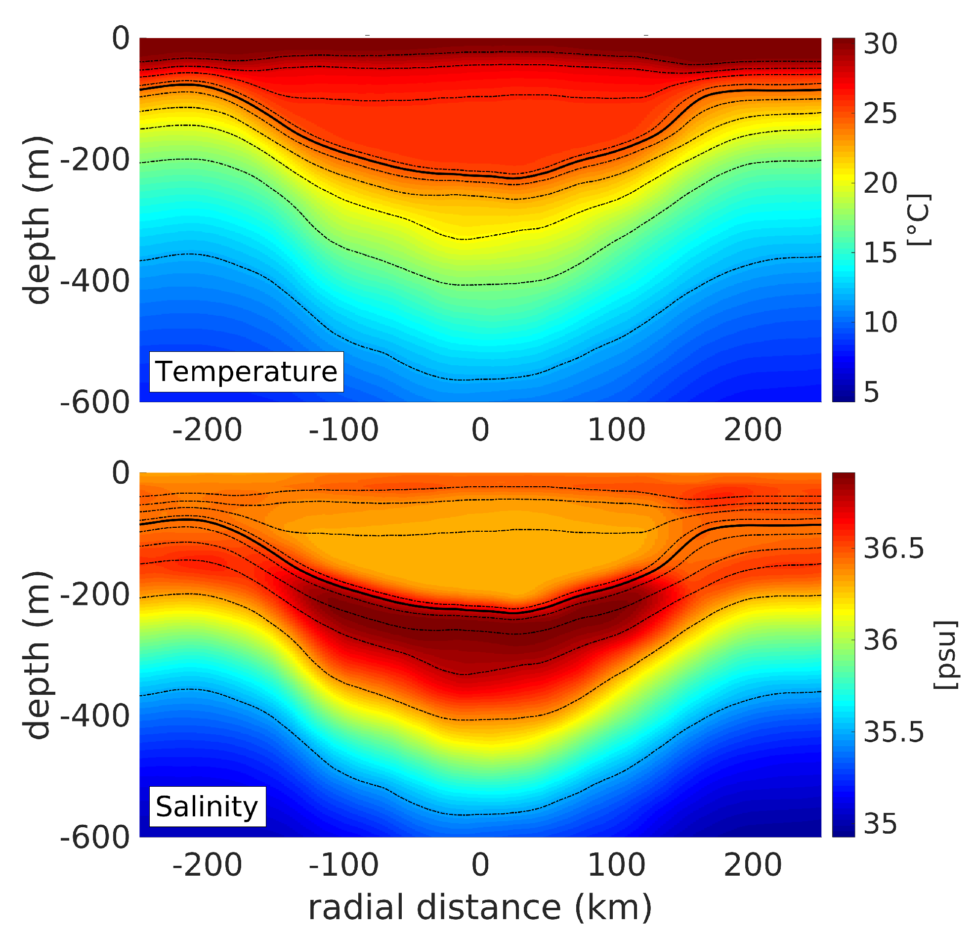
4.1. Thermohaline Structure

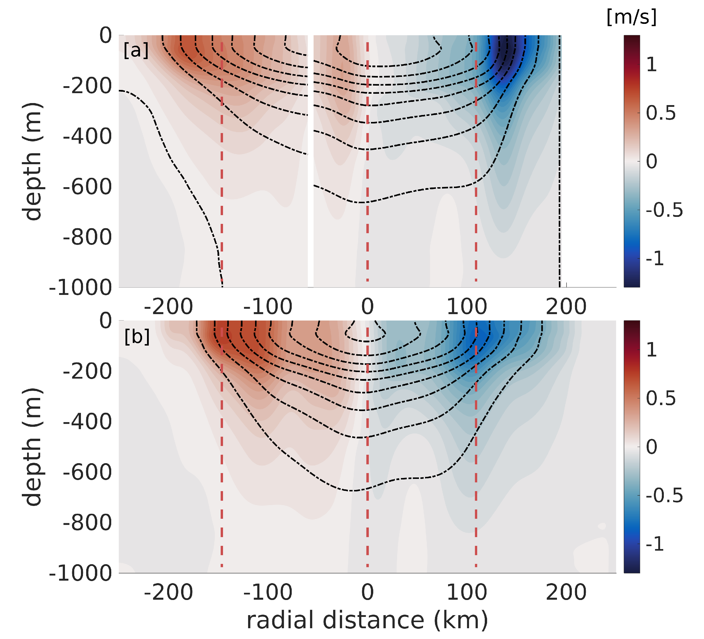
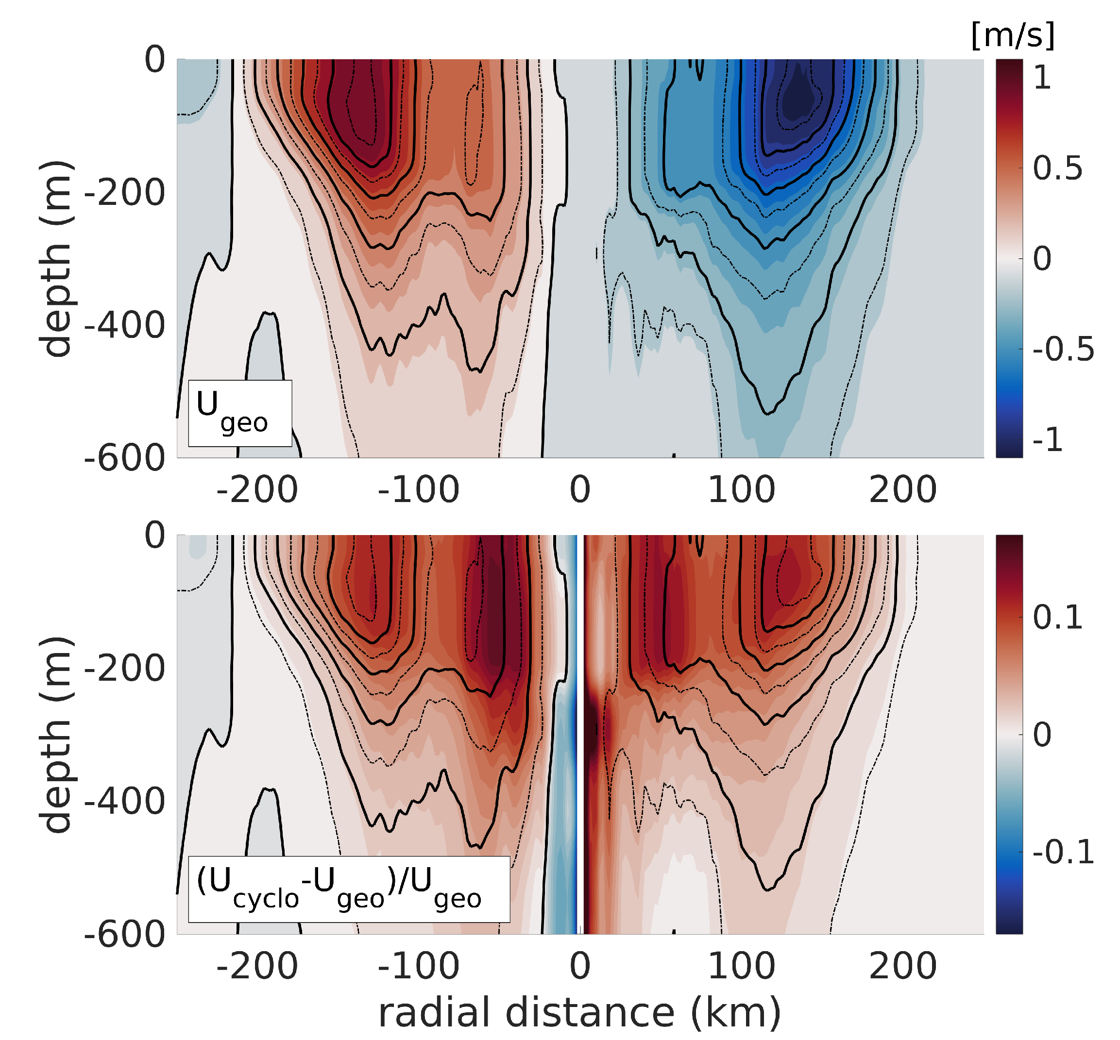
The vertical thermohaline structure of the LCR was described in detail in [9] and is only briefly recalled here. Figure 8 shows temperature and salinity sections across the LCR in relocated coordinates. The eddy is characterized by a warm and thick body of homogeneous temperature between 50 and 200 m. This thermostat splits the thermocline into an upper and a lower layer above and below the eddy core. The salinity structure is more complex, with a pancake-shaped high salinity core (≥36.9 psu) located in the lower part of the thermocline and a fresher homogeneous core above. The potential density structure is dominated by the temperature contribution: the isopycnals are deflected downward under the eddy core and are nearly parallel to the isotherms. The 25-isopycnal (1025 $\mathrm{kg}{\mathrm{m}}^{-3}$) delimits the lower edge of the thermostat and the frontier between the high and low salinity cores.

4.2. Velocity

The raw and corrected geostrophic velocity fields are compared in Figure 9. The former is computed using the original glider’s along-track coordinate, while the latter uses the altimetry-relocated coordinates described in Section 3.1. The original velocity field exhibits a strong asymmetry, with a positive velocity maximum of 0.55 $\mathrm{m}{\mathrm{s}}^{-1}$ at 180 km from the eddy center between the surface and 200 m, and a negative maximum of −1.25 $\mathrm{m}{\mathrm{s}}^{-1}$ at 140 km from the center. A secondary positive velocity maximum is evident at ~30 km from the rotation axis. The corrected velocity field is more symmetric, with similar maximal absolute values of ≈0.8 $\mathrm{m}{\mathrm{s}}^{-1}$ on both sides of the eddy. The secondary positive velocity maximum appears to be a spurious effect of the slow glider measuring a drifting eddy, and disappears when using the altimetry-relocation method. The diameter of the eddy (distance between both maxima) decreases from 320 km to 260 km when the relocation method is applied, meaning that the raw along-track glider coordinate is overestimating the eddy’s size by ≈23%.

The asymmetry of the original velocity field and the uncertainty on the exact position of the eddy’s center makes computing the cyclogeostrophic velocity in the glider’s along-track coordinate unreliable, because of the $1/r$ dependence in Equation (5). This constraint disappears in the symmetric velocity field computed from the relocated observations. A section of cyclogeostrophic velocity, as well as the relative difference in magnitude between geostrophic and cyclogeostrophic velocity, are shown in Figure 10. The cyclogeostrophic velocity reaches 1 $\mathrm{m}{\mathrm{s}}^{-1}$ on both sides of the eddy. The correction from geostrophic velocity consists in an increase of about $15\%$. Within two grid points from the rotation axis, the $1/r$ term in Equation (5) explodes while the azimuthal velocity is not strictly zero, yielding a spurious correction. Note that this effect is ubiquitous of computing gradient-wind balance with observations and is only localized at the rotation axis, so that it does not affect the important patterns of the velocity field.

4.3. Relative Vorticity and Strain

The vertical structure of the LCR’s relative vorticity is shown in Figure 11a. To avoid contamination by the velocity artifacts near the rotation axis discussed above, the first 3 grid points from the rotation axis were removed and vorticity was linearly re-interpolated to fill the gap. The eddy’s core is evident as an homogeneous negative relative vorticity bowl reaching −0.18f over the 25-isopycnal. Below, the vertical shear of azimuthal velocity results in a decrease of relative vorticity with depth, and relative vorticity is about 10 times smaller at 600 m than in the core. A surface intensified crown of positive relative vorticity surrounds the eddy’s core, consistent with the decrease of azimuthal velocity on the outer edge of the velocity maxima. The area of positive vorticity coincides with a well defined crown of intense shear strain (Figure 11b), reaching values of 0.2f on the outer flanks of the velocity maxima, at 140 to 170 km from the rotation axis. The strain crown is also near-surface intensified. Contours of the Okubo–Weiss parameter are also plotted in Figure 11, showing a sign reversal at the velocity maxima, negative values in the eddy core, and positive values outside, as expected from vorticity and strain dominated regions, respectively.

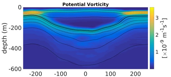
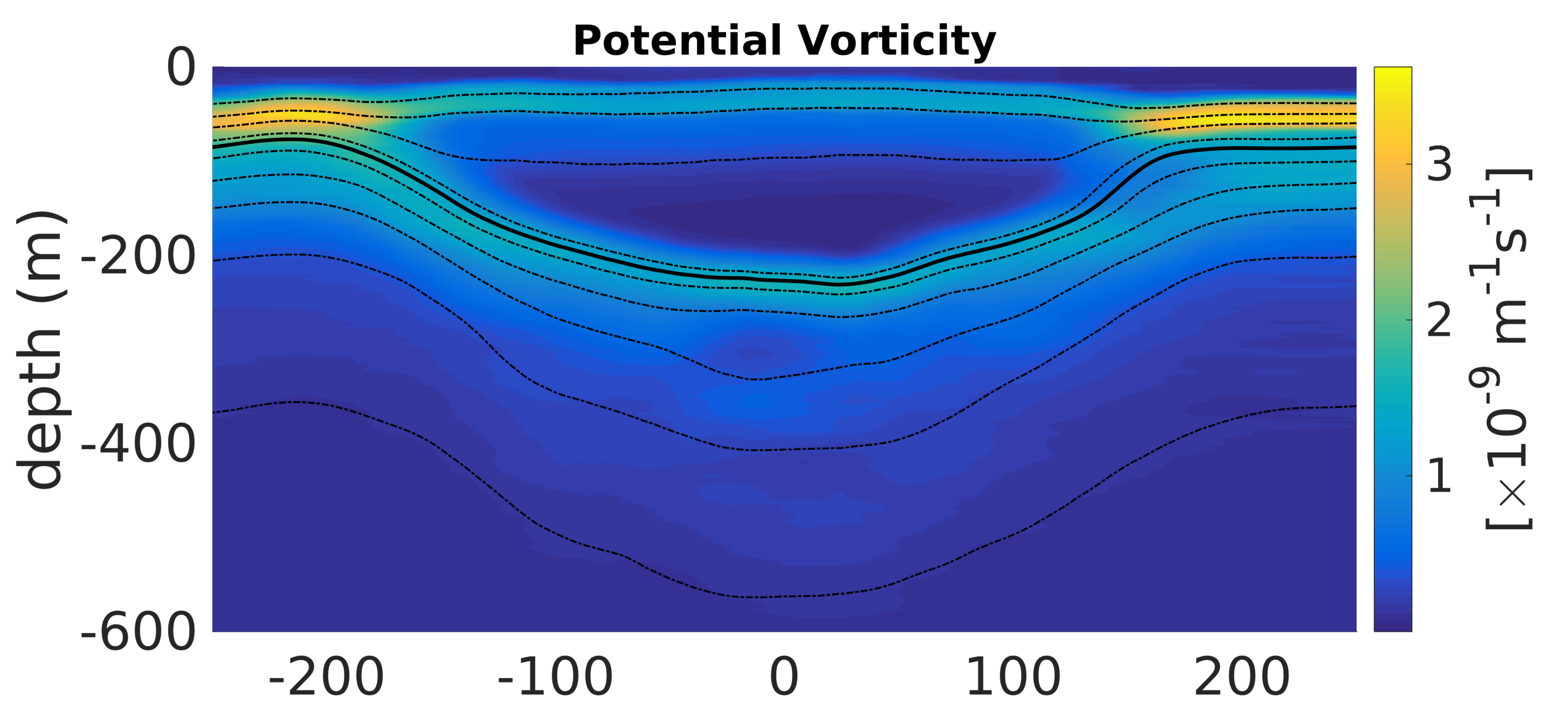
4.4. Potential Vorticity Structure

Figure 12 shows a vertical section of the vertical and baroclinic terms of Ertel’s PV. Outside of the LCR, vertical PV is maximum in the pycnocline and decreases with depth, consistent with a decrease in stratification. This vertical PV maximum separates into an upper and a lower branch, above and below the eddy’s core, consistent with the splitting of the pycnocline into a surface and deep pycnocline. The eddy’s core is characterized by a body of extremely low and homogeneous vertical PV (≈10${}^{-10}{\mathrm{m}}^{-1}{\mathrm{s}}^{-1}$), confined between the 25-isopycnal and the surface pycnocline and coincident with the location of the thermostat. The baroclinic term of Ertel’s PV is negligible everywhere (two orders of magnitude smaller than the vertical term), except in the pycnocline, on the outer edges of the core where two patches of higher PV are evident. This intensified baroclinic PV is associated with intense vertical shear and horizontal density gradients below the velocity maxima.

To quantify the respective contributions of relative vorticity, stratification and baroclinic PV in the PV signature of the LCR, the PVA was computed and decomposed into 4 terms (see details in Section 3.3). Vertical PVA and its three components are shown in Figure 13. The eddy core is evident as an homogeneous negative PVA bowl between the mixed layer and the lower pycnocline materialized by the 25-isopycnal (Figure 13a). The stretching term exhibits the exact same pattern and magnitude, while the vorticity term (Figure 13c) is 4 to 5 times smaller. The nonlinear term (Figure 13d) has an opposite contribution to PVA and consists in a positive PVA bowl above the lower pycnocline, whose shape and size closely match the vorticity term. Figure 14 shows vertical profiles of PVA averaged over the inner-core of the eddy ($r\in$ (0–100) km) and over the peripheral region ($r\in$ (100–150) km). The stretching term entirely dominates PVA in both regions. The vorticity term, despite having a non-negligible contribution to PVA is mostly compensated by the nonlinear term, which has a similar vertical distribution and magnitude, but an opposite sign. As expected, the contribution of the baroclinic term is larger near the outer edge than in the inner core, but however remains negligible. The potential enstrophy associated with the stretching, vorticity, nonlinear, and baroclinic terms normalized by the total potential enstrophy is of 0.94, 0.04, 0.02, and 0.006, respectively. The associated enstrophy Burger number is $B_q=0.2$.

Most oceanic eddies are subject to baroclinic instability and LCRs were shown to exhibit elliptic patterns [27], which is reminiscent of azimuthal mode 2 unstable modes, commonly associated with baroclinic instability [38,39,40]. The Charney–Stern equivalent criterion for baroclinic instability in circular vortices is that the radial PV gradient must change sign somewhere in the water column [41]. Figure 15 shows a vertical section of the along-isopycnal PV gradient and the respective contributions of the gradients of vortex stretching, relative vorticity, and nonlinear term. The PV gradient is maximal at the edges of the LCR, near the velocity maxima. On both edges, a sign reversal of the PV gradient is evident at ~140 km from the rotation axis between 100 and 200 m depth, in the pycnocline. Several sign reversals with lesser amplitudes are also evident in the central core of the LCR within the pycnocline. Examination of the vortex stretching, relative vorticity, and nonlinear term gradients on Figure 15b–d suggests that the PV gradient reversal is essentially driven by the vortex stretching gradient, since the relative vorticity gradient does not changes sign along the vertical direction, and the sign reversals observed in the gradient of the non-linear term below the central part of the eddy core are associated with gradients that are one order of magnitude smaller than vortex stretching gradients. Vertical profiles of the PV gradient and its components averaged over three areas of evident sign reversal are shown in Figure 16. Examination of these profiles confirms that the sign change of the PV gradient over the vertical is driven by vortex stretching, and that relative vorticity gradients do not change sign, and are mostly compensated by gradients of the nonlinear term anyway. Again, the baroclinic term has a negligible contribution here.

4.5. Energetics

As understanding the contribution of vortex stretching and relative vorticity is important to understand LCR’s dynamics, assessing the distribution of energy density across the eddy and its partition between kinetic and potential energy is of interests. Figure 17a–c shows sections of available potential energy density (APED), kinetic energy density (KED), and total energy density (TED), respectively. Total energy density is concentrated in the eddy core at the base of the thermostat, above the lower pycnocline, and decreases dramatically with depth. There is little energy density in the LCR’s mixed layer. Available potential energy appears to largely dominate over kinetic energy, with maxima of 2000 and 500 $\mathrm{J}{\mathrm{m}}^{-3}$ located in the core and at the periphery, respectively. The contribution of kinetic energy to total energy is only barely noticeable around the near-surface velocity maxima, at about 140 km from the rotation axis. The total energy of the LCR is of $1.9\times {10}^{16}$ J from which kinetic energy accounts for $5.1\times {10}^{15}$ J and available potential energy for $1.4\times {10}^{16}$ J, resulting in an Energy Burger number of $B_e=0.36$.

5. Discussion

5.1. The Relocation Method

In this observational study, we introduced a new method to compensate for the lack of synopticity of glider surveys when sampling fast-drifting eddies. By taking advantage of the synopticity of along-track altimetry data, this method allows to relocate gliders dives in a synoptic frame of reference. The method shares some similarity with the commonly used composite method [42,43,44], which consists of detecting a number of eddies using altimetry and to use all available in situ data, relocated in non-dimensional radial coordinate, to build climatological means of eddies vertical structure. However, rather than reconstructing smooth vertical sections averaged over tens or hundreds of eddies, here, we use one single along-track SSH profile acquired simultaneously with the glider survey, to relocate precisely each glider’s dive. The relocation method thus aims to reconstruct one single, truly synoptic picture of the eddy. The major advantage of this method, beyond recovering the true spatial scales of the sampled structure, is to recover a reliable horizontal coordinate to compute radial gradients that are otherwise strongly contaminated by fluctuations of the glider’s velocity and eddy’s drift speed. Using the relocation method, the eddy also recovers its azimuthal symmetry and its rotation axis can easily be identified. These criteria are crucial when attempting to compute cyclogeostrophic velocity and relative vorticity from in situ data, especially in the vicinity of the rotation axis.

It is, however, important to acknowledge some limitations of the method. First, the spatial resolution of along-track altimetry remains coarser than the glider’s (7 km vs. ≈2 km), so that some details of the eddy’s structure are lost in the process. It should, however, be mentioned that, to compute geostrophic velocity from glider data (or from any in situ hydrographic transect), it is crucial to filter the observations to a scale of O(30 km) [3]. The low-pass filtering effect of relocating the glider profiles on a smoother altimetry profile is thus not much different than that necessary when interpolating the glider data on a regular grid to compute geostrophic velocity. In any case, we should be clear about the fact that the resolution of the relocated glider transect does not allow us to access the details level necessary to study sub-mesoscale frontal processes such as symmetric instability. For instance, the baroclinic PV component might be underestimated here, in comparison with raw glider data. The relevancy of the method thus depends on the desired balance between accuracy of the horizontal coordinate and level of details.

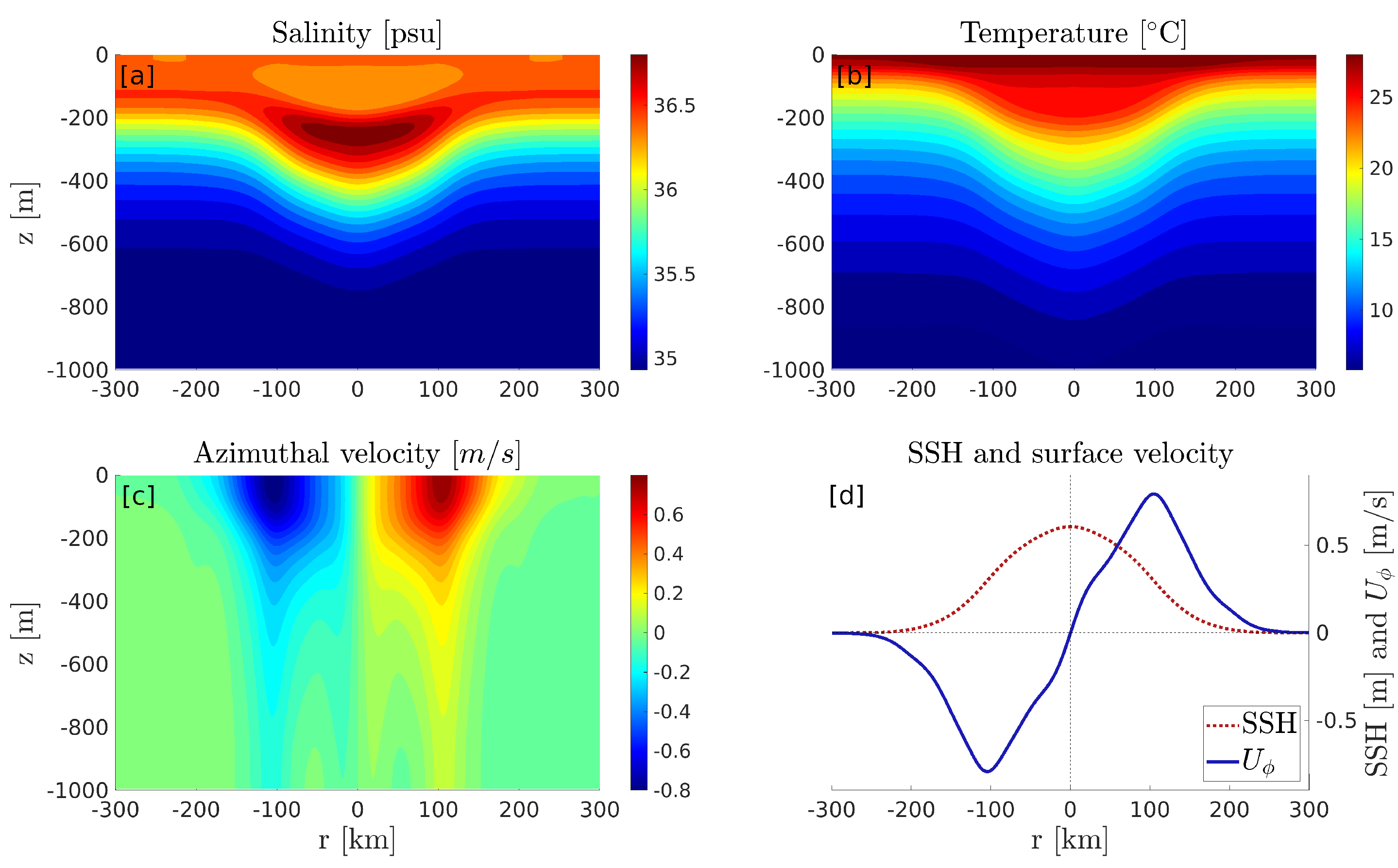
5.2. The LCR’s Vertical Structure

One of the most striking feature of LCR’s vertical structure is the clear dominance of the vortex stretching contribution to PVA over that of relative vorticity. While this might sound surprising, given the intense currents associated with LCRs (velocity maxima $>1\mathrm{m}{\mathrm{s}}^{-1}$), the unusually large size of these eddies yields only modest values of relative vorticity (<$0.2f$ here). Most importantly, the exceptionally weak stratification in the eddy’s core, that is referred to as the thermostad or pycnostad drives intense isopycnal Brunt-Väisälä frequency anomalies, responsible for large vortex stretching anomalies. Note that, not only is the stretching term about 5 times larger than the relative vorticity term ($B_q\approx 0.2$), but the nonlinear term also largely cancels the effect of the vorticity term, as the Brunt–Väisälä frequency anomaly is of the same order of magnitude as the mean (near-zero $N^2$ within the eddy’s core), and of opposite sign. This results in the stretching term being nearly equal to the full PVA, which means that, on the f-plane and at the scales considered here (O[$R_d$]), the Brunt–Väisälä frequency is a close proxy for Ertel’s PV, and can be considered as a nearly conservative tracer in the absence of diabatic processes. This could have convenient applications in the case of trying to infer PV with hydrographic data in the absence of a reliable velocity reference (e.g., no information on the level of no motion), or when using uncertain horizontal coordinates (poor synopticity as in the case of a slow glider measuring a fast-drifting eddy). Again, it is important to note that we are considering scales of motion of the order of the Rossby radius or larger, i.e., scales at which geostrophic velocity can be inferred from the density distribution [3]. At smaller scales, one should expect an important contribution of sub-mesoscale processes, associated with sharp fronts and high Rossby number eddies embedded in the large LCR [10], and locally significant contributions of the relative vorticity and baroclinic PV terms.

Similar to the skewed contributions of the PVA terms, we found a strong asymmetry in the partition of energy between APE and KE. While equipartition is expected in geostrophic turbulence’s mesoscale eddies, here, APE largely dominates over KE (≈3 times larger), with an energy Burger number $B_e$ of 0.36. This low value of $B_e$ is consistent with previous estimates [45] in an LCR (0.25), and more generally, is consistent with most measured warm-core rings (0.17 in a Gulf stream ring [23,46], 0.18 in an Aghulas ring [21], and 0.4 to 1 in Brazil current rings [20]). LCRs (and warm-core rings in general) are thus not only remarkable by their intense currents, but also by their large reservoirs of available potential energy, which could possibly contribute to their longevity: even if kinetic energy dissipated through shear instability or interaction with the surrounding geostrophic turbulence at the edges of the eddy, the APE reservoir could provide the necessary energy to maintain their circulation. The authors of [23,45], however, showed that this APE excess, relative to KE, was a characteristics of young rings, and that APE decays with time, possibly converging towards equipartition of energy for old rings.

Note that the APE reservoir seems to be located in a safe place: as shown in the depth averaged profiles of energy density in Figure 18, APE density is concentrated within the core of the eddy, where the OW parameter is negative and tracers are expected to be well conserved [31,32]. One should however note that, since the Charney–Stern criterion is verified in this eddy, baroclinic instability is to be expected, and could be an efficient way to transform the eddy’s APE into eddy kinetic energy (EKE), thus diminishing the reservoir. Linear stability analysis and numerical modeling works by [47,48,49] previously showed that, despite being long-lived, warm-core rings were unstable structures. Splitting of LCRs in the central GoM was reported in [50], resulting in the decay and death of the eddies. Low wavenumber baroclinic instability could very well be a possible process for the splitting of LCRs, prematurely ending their long life cycle. Although this is beyond the scope of this observational study, linear stability analysis and numerical modeling of LCRs, similar to [47,48,49], but using the observed vertical structure reported here, would be necessary to go beyond these speculations.

The large APE reservoir in the LCR is essentially related to the homogeneous warm anomaly within its core. LCR’s heat input towards the inner GoM was recently estimated by [24], using a combination of in situ observations and satellite altimetry. Between 1993 and 2017, LCRs carried 16.5 ZJ into the GoM, which would be equivalent to a yearly mean surface heat flux of 14 $\mathrm{W}{\mathrm{m}}^{-2}$ over the whole GoM’s surface. By examining the decay of LCR’s heat content, they showed that heat was primarily transferred to the surrounding GoM water rather than towards the atmosphere. Understanding the processes by which LCRs release their heat seems crucial to understand the decadal evolution of sea level rise in the GoM due to steric effects. Here, we find that 74% of the heat anomaly associated with the LCR lays inside the coherent core, where OW is negative and tracers are expected to be conserved. This leaves 26% of the heat anomaly in the strain-dominated crown where dispersion is expected to be higher and the LCR’s thermohaline properties might be subject to stirring and mixing with the surrounding water masses. Note however that, although the thermohaline anomalies are located in a presumably coherent area of the eddy, the latter could undergo baroclinic instability that could eventually fragment it and favor tracer dispersion. Note also that, while the resolution of our relocated observations does not resolve sub-mesoscale frontal processes, such as symmetric instability [51], the latter were shown to occur in other mesoscale eddies [52,53,54,55] and could also occur in LCRs and contribute to the mixing of their tracers. Finally, the occurrence of layering at the periphery of the sampled LCR [11], associated with elevated mixing [12] might also act in eroding the tracer anomalies, and contribute to the decay of the eddy, as observed in intra-thermocline lenses in the North Atlantic [37].

6. Summary

The main conclusions of this study can be summarized as follows.

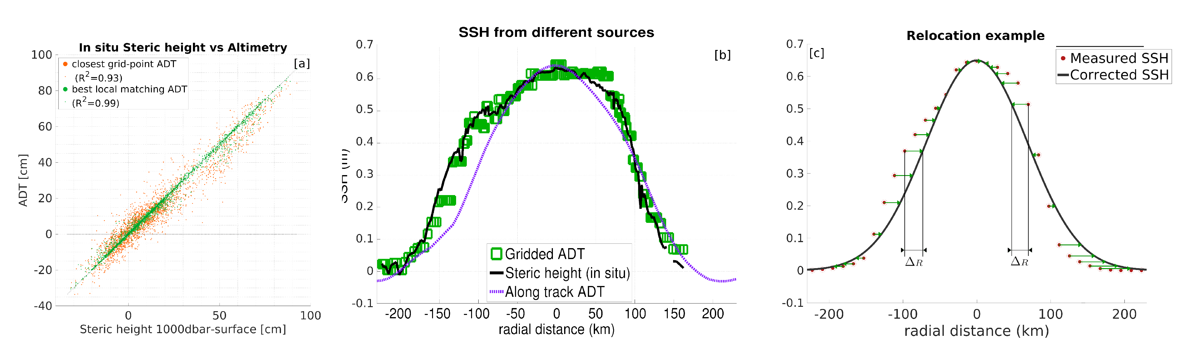
• A new altimetry-based method to relocate gliders observations in a synoptic frame of reference was designed and applied to recent observations of a Loop Current ring in the Gulf of Mexico.
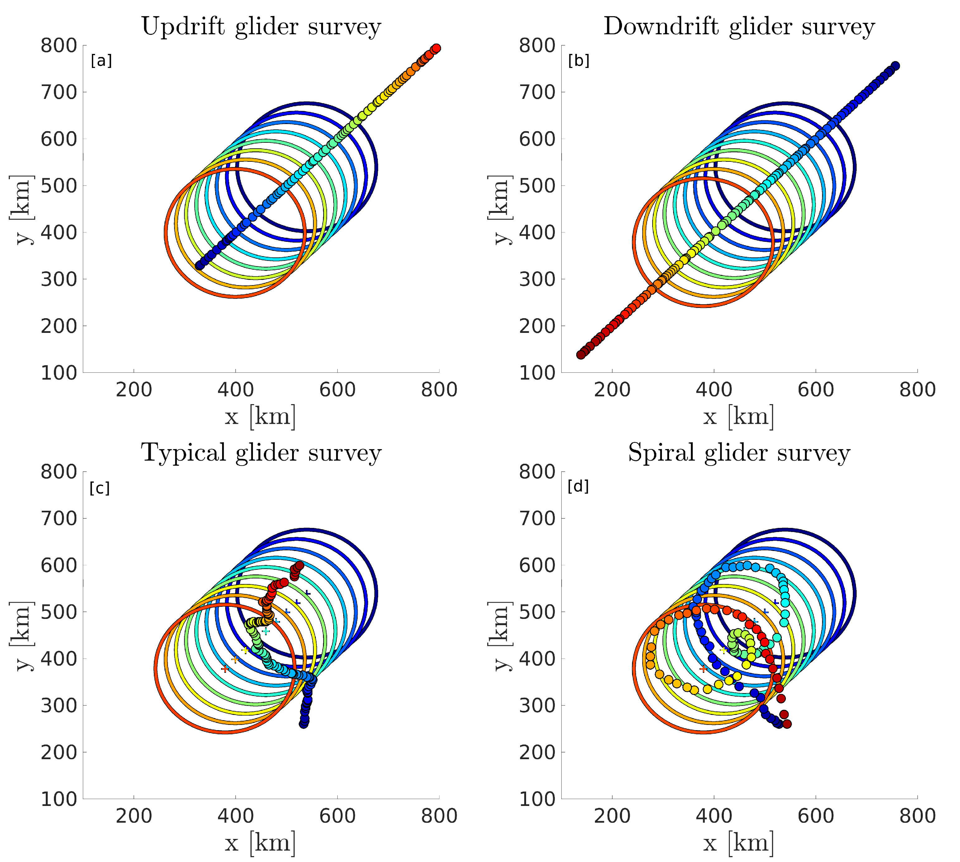
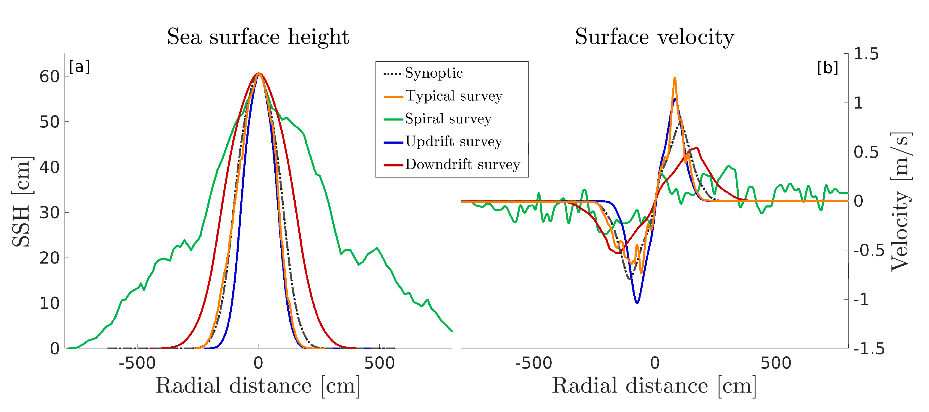
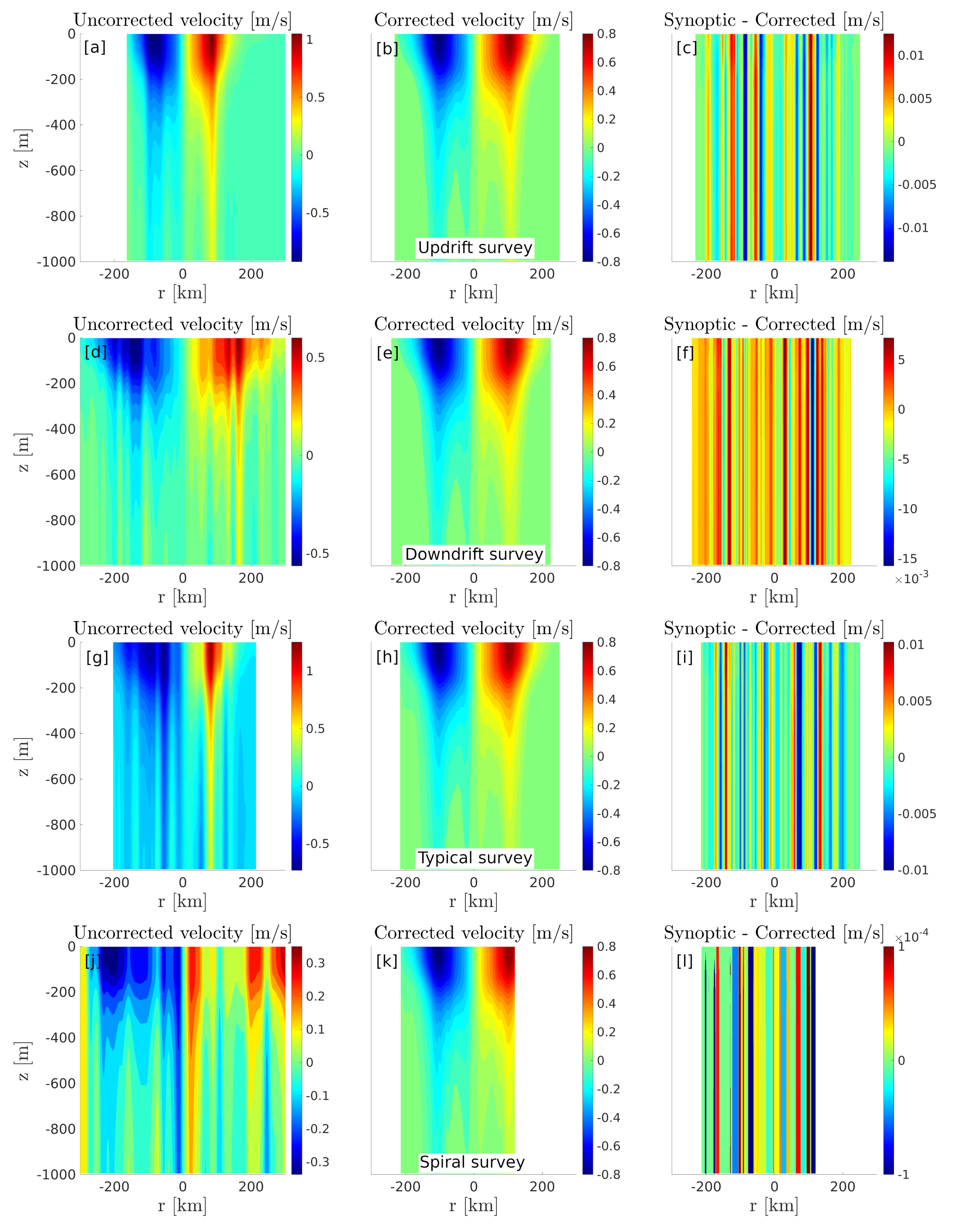
• The method was tested using an analytical anticyclonic eddy drifting on the $\beta$-plane, and shown to recover the exact vertical structure of the eddy, whatever the sampling strategy, in the ideal case of a stable and circular eddy.
• The method was successful in correcting the errors in horizontal thermohaline gradients, related to the lack of synopticity of glider surveys.
• The relocation method also allows to precisely locate the eddy’s rotation axis, yielding more reliable estimates of cyclo-geostrophic velocity, relative vorticity, and shear strain.
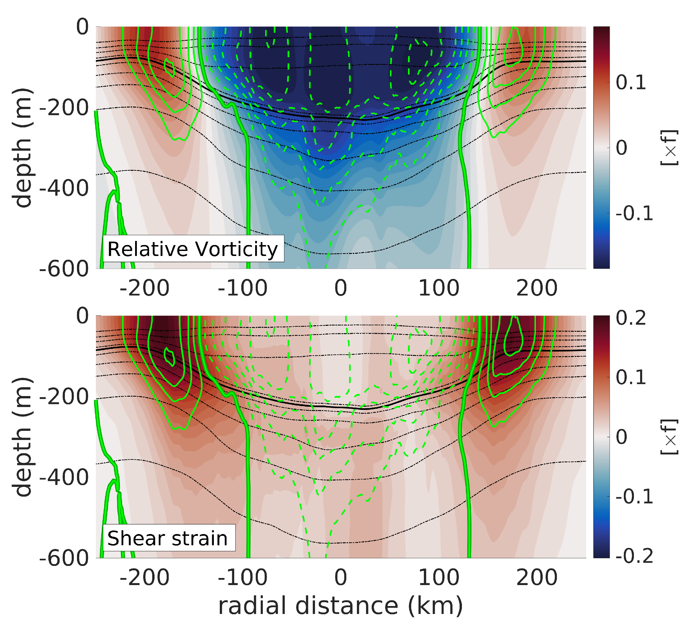
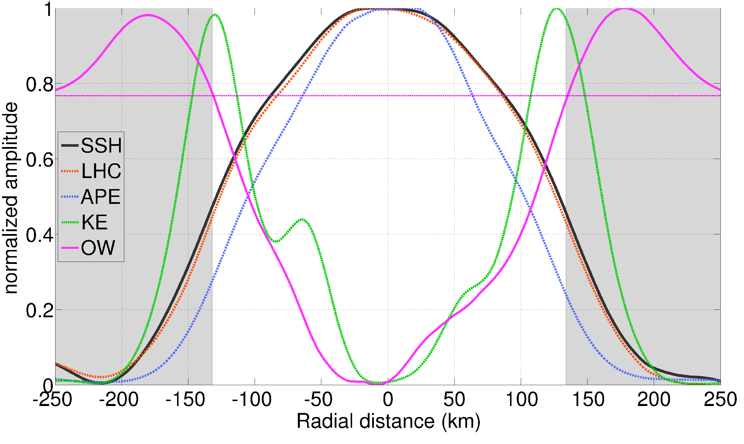
• The warm core ring consisted of a bowl of homogeneous negative relative vorticity, surrounded by a crown of positive shear strain, resulting in a negative Okubo–Weiss parameter in the core and positive at the periphery.
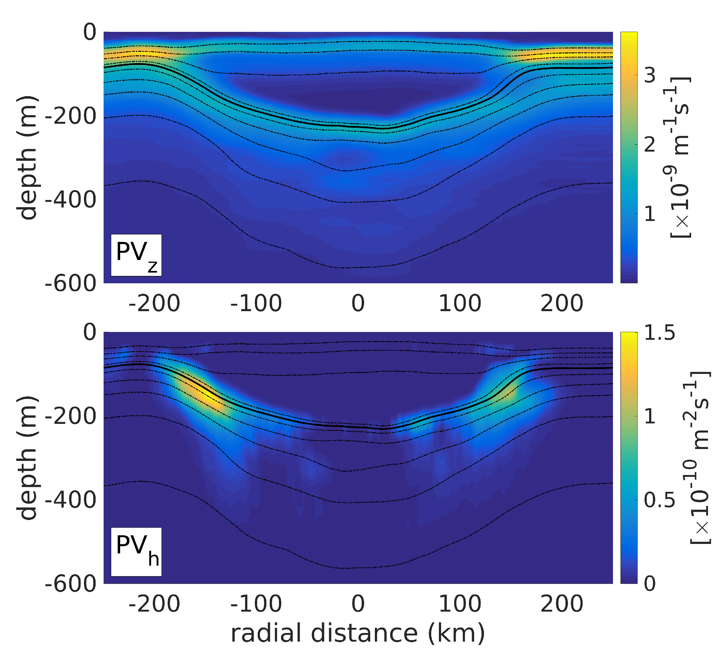
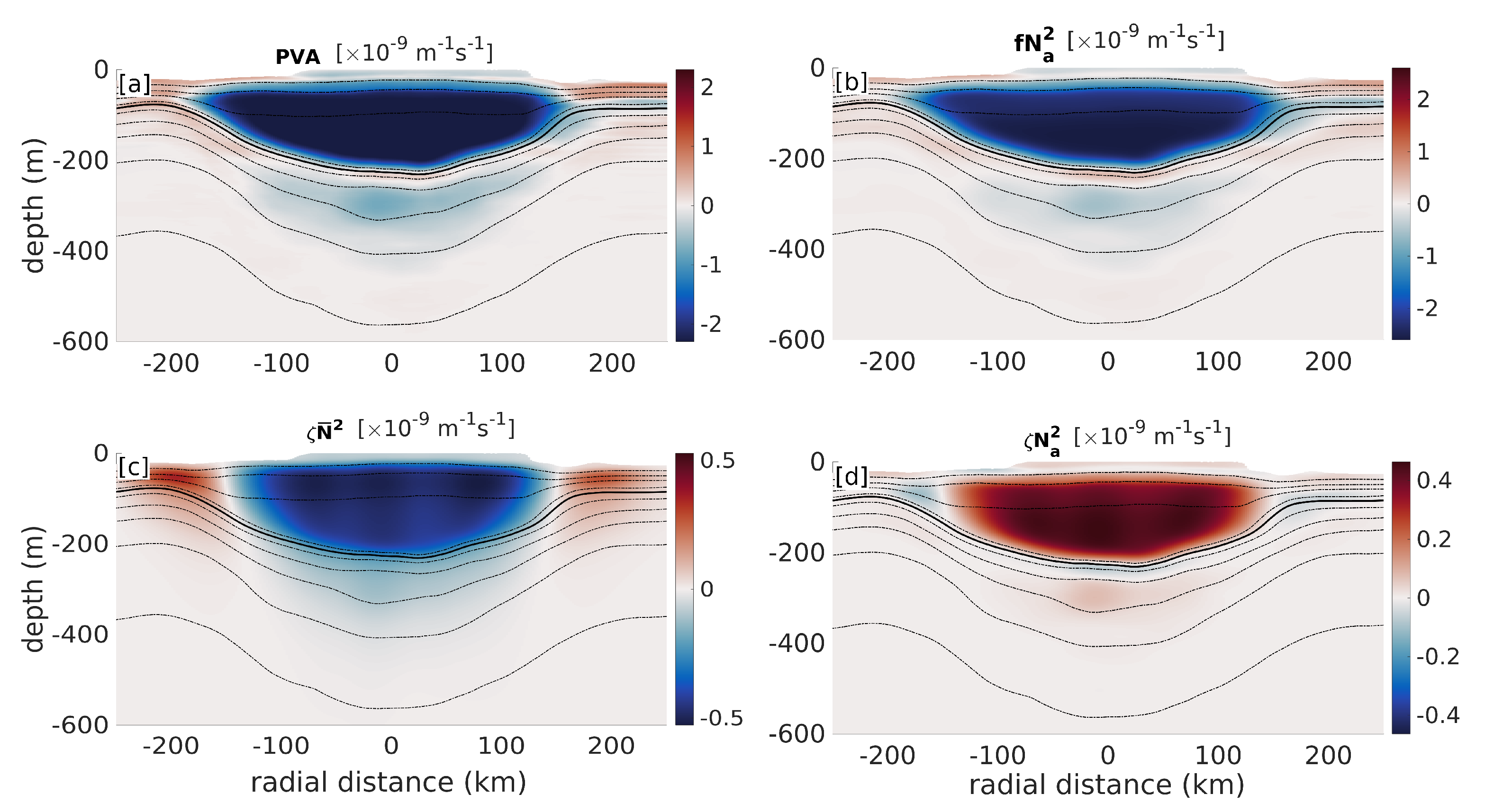
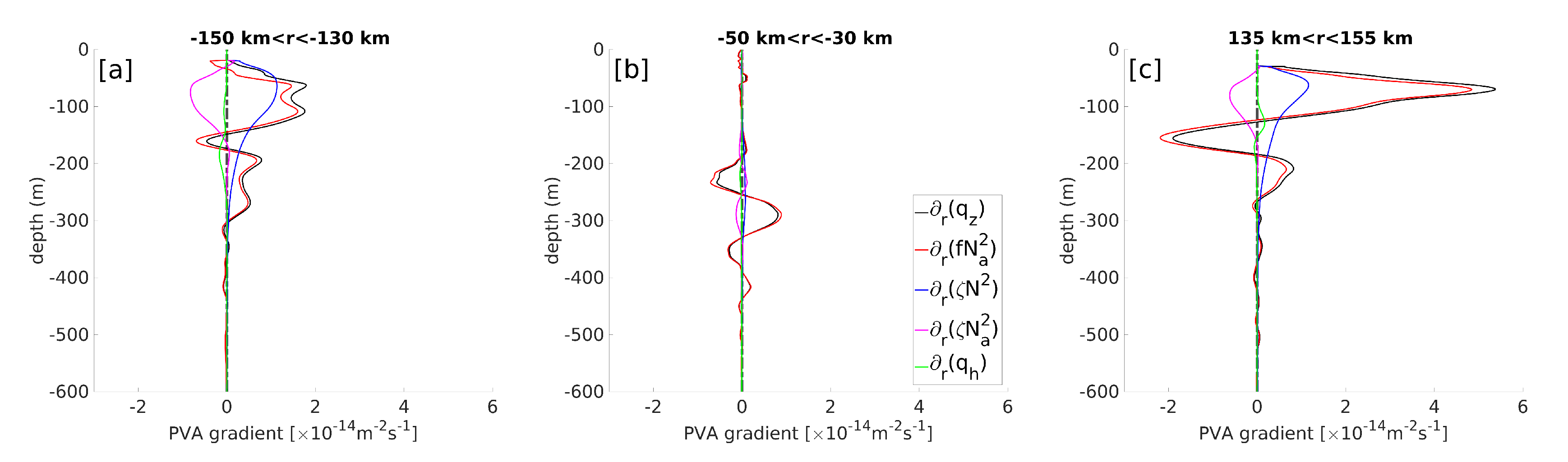
• The PV structure of the warm-core ring is largely dominated by vortex stretching.
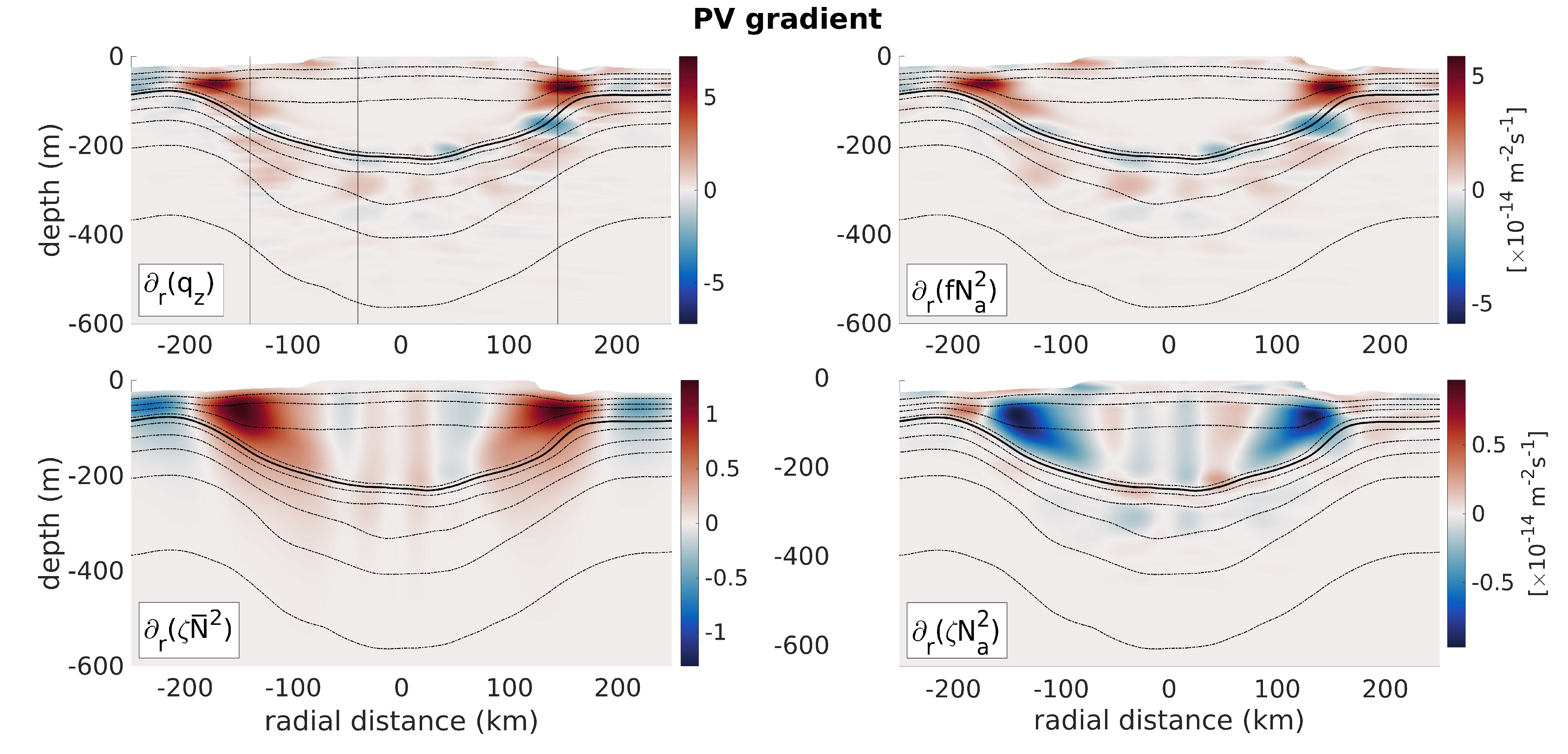
• The along-isopycnal radial PV gradient is also dominated by gradients of the vortex stretching term.
• Sign-changes of the PV-gradient suggests that the warm core ring might be baroclinically unstable.
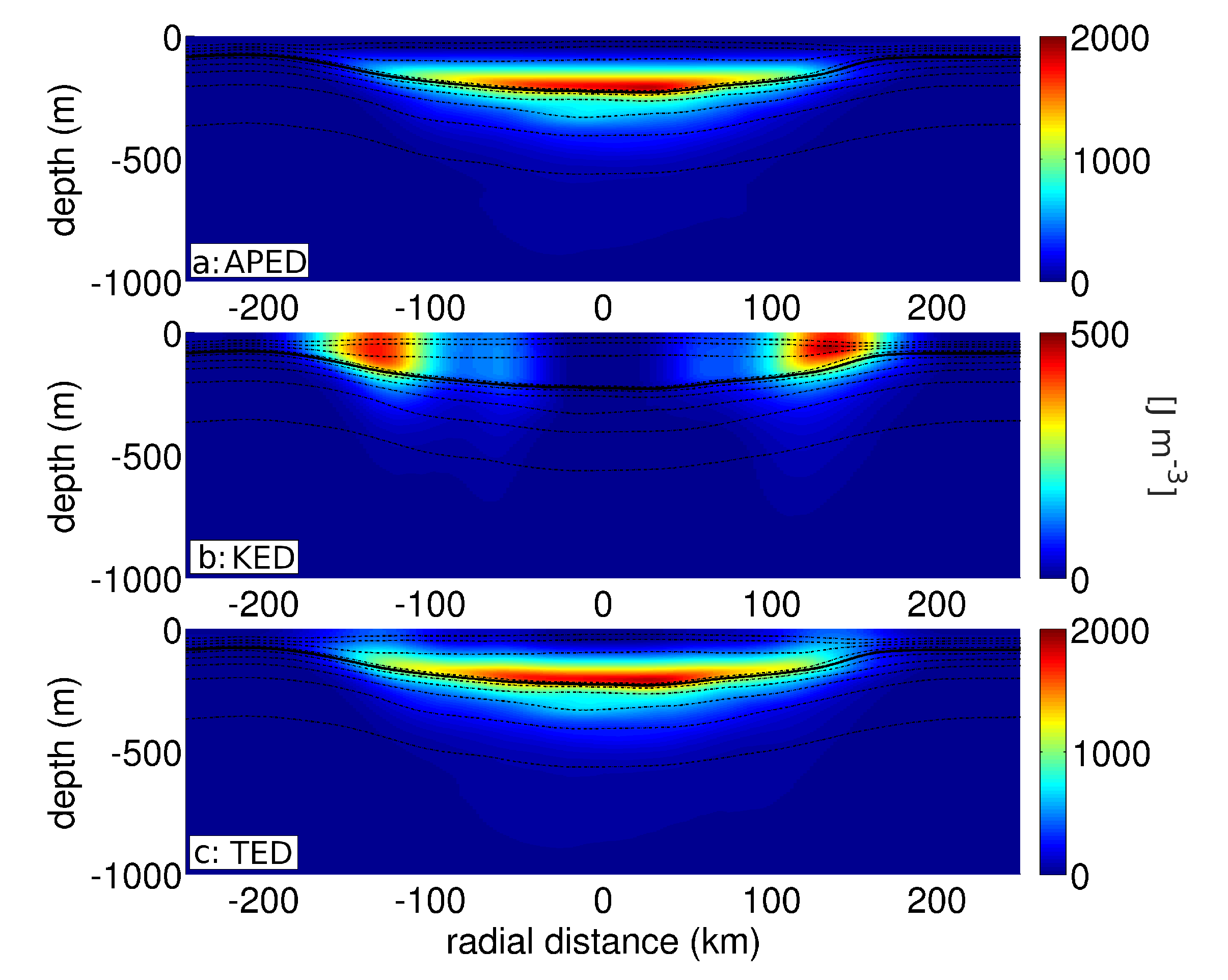
• The energy density partition revealed a clear dominance of available potential energy over kinetic energy.
• Available potential energy density is mostly contained within the vorticity-dominated core of the warm-core ring (negative Okubo–Weiss), where properties are expected to be well conserved. This might possibly contribute to its longevity.

References

1. Testor, P.; de Young, B.; Rudnick, D.L.; Glenn, S.; Hayes, D. OceanGliders: A component of the integrated GOOS. Front. Mar. Sci. 2019, 6, 422. [Google Scholar] [CrossRef] [Green Version]
2. Rudnick, D.L.; Davis, R.E.; Eriksen, C.C.; Fratantoni, D.M.; Perry, M.J. Underwater gliders for ocean research. Mar. Technol. Soc. J. 2004, 38, 73–84. [Google Scholar] [CrossRef]
3. Rudnick, D.L.; Cole, S.T. On sampling the ocean using underwater gliders. J. Geophys. Res. 2011, 116, C08010. [Google Scholar] [CrossRef] [Green Version]
4. Rudnick, D.L. Ocean Research Enabled by Underwater Gliders. Annu. Rev. Mar. Sci. 2016, 8, 519–541. [Google Scholar] [CrossRef] [PubMed]
5. Rudnick, D.L.; Johnston, T.M.S.; Sherman, J.T. High-frequency internal waves near the Luzon Strait observed by underwater gliders. J. Geophys. Res. 2013, 118, 774–784. [Google Scholar] [CrossRef]
6. Todd, R.E. Gulf Stream Mean and Eddy Kinetic Energy: Three-Dimensional Estimates From Underwater Glider Observations. Geophys. Res. Lett. 2021, 48, 2020GL090281. [Google Scholar] [CrossRef]
7. Kolodziejczyk, N.; Testor, P.; Lazar, A.; Echevin, V.; Krahmann, G.; Chaigneau, A.; Gourcuff, C.; Wade, M.; Faye, S.; Estrade, P.; et al. Subsurface Fine-Scale Patterns in an Anticyclonic Eddy Off Cap-Vert Peninsula Observed From Glider Measurements. J. Geophys. Res. Ocean. 2018, 123, 6312–6329. [Google Scholar] [CrossRef]
8. Rudnick, D.L.; Gopalakrishnan, G.; Cornuelle, B.D. Cyclonic Eddies in the Gulf of Mexico: Observations by Underwater Gliders and Simulations by Numerical Model. J. Phys. Oceanogr. 2015, 45, 313–326. [Google Scholar] [CrossRef]
9. Meunier, T.; Pallás-Sanz, E.; Tenreiro, M.; Portela, E.; Ochoa, J.; Ruiz-Angulo, A.; Cusí, S. The vertical structure of a Loop Current Eddy. J. Geophys. Res. Ocean. 2018, 123, 6070–6090. [Google Scholar] [CrossRef]
10. Meunier, T.; Tenreiro, M.; Pallàs-Sanz, E.; Ochoa, J.; Ruiz-Angulo, A.; Portela, E.; Cusí, S.; Damien, P.; Carton, X. Intrathermocline Eddies Embedded within an Anticyclonic Vortex Ring. Geophys. Res. Lett. 2018, 45, 7624–7633. [Google Scholar] [CrossRef] [Green Version]
11. Meunier, T.; Pallàs Sanz, E.; Tenreiro, M.; Ochoa, J.; Ruiz Angulo, A.; Buckingham, C. Observations of Layering under a Warm-Core Ring in the Gulf of Mexico. J. Phys. Oceanogr. 2019, 49, 3145–3162. [Google Scholar] [CrossRef]
12. Molodtsov, S.; Anis, A.; Amon, R.M.W.; Perez-Brunius, P. Turbulent Mixing in a Loop Current Eddy from Glider-Based Microstructure Observations. Geophys. Res. Lett. 2020, 47, e88033. [Google Scholar] [CrossRef]
13. Ichiye, T. Circulation and water-mass distribution in the Gulf of Mexico. J. Geophys. Res. 1959, 64, 1109–1110. [Google Scholar]
14. Elliott, B.A. Anticyclonic Rings in the Gulf of Mexico. J. Phys. Oceanogr. 1982, 12, 1292–1309. [Google Scholar] [CrossRef] [Green Version]
15. Vukovich, F.M. An updated evaluation of the Loop Current’s eddy-shedding frequency. J. Geophys. Res. 1995, 100, 8655–8659. [Google Scholar] [CrossRef]
16. Liu, Y.; Wilson, C.; Green, M.A.; Hughes, C.W. Gulf Stream Transport and Mixing Processes via Coherent Structure Dynamics. J. Geophys. Res. 2018, 123, 3014–3037. [Google Scholar] [CrossRef]
17. Richardson, P. Gulf stream rings. In Eddies in Marine Science; Springer: Berlin/Heidelberg, Germany, 1983; pp. 19–45. [Google Scholar] [CrossRef]
18. Li, L.; Nowlin, W.D.; Jilan, S. Anticyclonic rings from the Kuroshio in the South China Sea. Deep Sea Res. Part I Oceanogr. Res. 1998, 45, 1469–1482. [Google Scholar] [CrossRef]
19. Sasaki, Y.N.; Minobe, S. Climatological Mean Features and Interannual to Decadal Variability of Ring Formations in the Kuroshio Extension Region. In AGU Fall Meeting Abstracts; Springer: Tokyo, Japan, 2014; Volume 2014, p. OS41F-07. [Google Scholar] [CrossRef] [Green Version]
20. Fratantoni, D.M.; Johns, W.E.; Townsend, T.L. Rings of the North Brazil Current: Their structure and behavior inferred from observations and a numerical simulation. J. Geophys. Res. 1995, 100, 10633–10654. [Google Scholar] [CrossRef]
21. Olson, D.B.; Evans, R.H. Rings of the Agulhas current. Deep Sea Res. A 1986, 33, 27–42. [Google Scholar] [CrossRef]
22. Wang, Y.; Beron-Vera, F.J.; Olascoaga, M.J. The life cycle of a coherent Lagrangian Agulhas ring. J. Geophys. Res. 2016, 121, 3944–3954. [Google Scholar] [CrossRef] [Green Version]
23. Olson, D.B.; Schmitt, R.W.; Kennelly, M.; Joyce, T.M. A two-layer diagnostic model of the long-term physical evolution of warm-core ring 82B. J. Geophys. Res. 1985, 90, 8813–8822. [Google Scholar] [CrossRef]
24. Meunier, T.; Sheinbaum, J.; Pallàs-Sanz, E.; Tenreiro, M.; Ochoa, J.; Ruiz-Angulo, A.; Carton, X.; de Marez, C. Heat Content Anomaly and Decay of Warm-Core Rings: The Case of the Gulf of Mexico. Geophys. Res. Lett. 2020, 47, e85600. [Google Scholar] [CrossRef]
25. Cooper, C.; Forristall, G.Z.; Joyce, T.M. Velocity and hydrographic structure of two Gulf of Mexico warm-core rings. J. Geophys. Res. 1990, 95, 1663–1679. [Google Scholar] [CrossRef]
26. Hamilton, P.; Leben, R.; Bower, A.; Furey, H.; Pérez-Brunius, P. Hydrography of the Gulf of Mexico Using Autonomous Floats. J. Phys. Oceanogr. 2018, 48, 773–794. [Google Scholar] [CrossRef]
27. Hamilton, P.; Fargion, G.S.; Biggs, D.C. Loop Current Eddy Paths in the Western Gulf of Mexico. J. Phys. Oceanogr. 1999, 29, 1180–1207. [Google Scholar] [CrossRef]
28. Hoskins, B.J.; McIntyre, M.E.; Robertson, A.W. On the use and significance of isentropic potential vorticity maps. Q. J. R. Meteorol. Soc. 1985, 111, 877–946. [Google Scholar] [CrossRef]
29. Penven, P.; Halo, I.; Pous, S.; Marié, L. Cyclogeostrophic balance in the Mozambique Channel. J. Geophys. Res. 2014, 119, 1054–1067. [Google Scholar] [CrossRef] [Green Version]
30. Weiss, J. The dynamics of enstrophy transfer in two-dimensional hydrodynamics. Phys. D Nonlinear Phenom. 1991, 48, 273–294. [Google Scholar] [CrossRef]
31. Isern-Fontanet, J.; Font, J.; García-Ladona, E.; Emelianov, M.; Millot, C.; Taupier-Letage, I. Spatial structure of anticyclonic eddies in the Algerian basin (Mediterranean Sea) analyzed using the Okubo Weiss parameter. Deep Sea Res. Part II Top. Stud. Oceanogr. 2004, 51, 3009–3028. [Google Scholar] [CrossRef]
32. Provenzale, A. Transport by Coherent Barotropic VORTICES. Annu. Rev. Fluid Mech. 1999, 31, 55–93. [Google Scholar] [CrossRef] [Green Version]
33. Lorenz, E.N. Available Potential Energy and the Maintenance of the General Circulation. Tellus Ser. A 1955, 7, 157–167. [Google Scholar] [CrossRef]
34. Holliday, D.; McIntyre, M.E. On potential energy density in an incompressible, stratified fluid. J. Fluid Mech. 1981, 107, 221–225. [Google Scholar] [CrossRef]
35. Huang, R.X. Available potential energy in the world’s oceans. J. Mar. Res. 2005, 63, 141–158. [Google Scholar] [CrossRef]
36. D’Asaro, E.A. Observations of small eddies in the Beaufort Sea. J. Geophys. Res. 1988, 93, 6669–6684. [Google Scholar] [CrossRef]
37. Armi, L.; Hebert, D.; Oakey, N.; Price, J.F.; Richardson, P.L.; Thomas Rossby, H.; Ruddick, B. Two Years in the Life of a Mediterranean Salt Lens. J. Phys. Oceanogr. 1989, 19, 354–370. [Google Scholar] [CrossRef]
38. Saunders, P.M. The Instability of a Baroclinic Vortex. J. Phys. Oceanogr. 1973, 3, 61–65. [Google Scholar] [CrossRef] [Green Version]
39. Flierl, G.R. On the instability of geostrophic vortices. J. Fluid Mech. 1988, 197, 349–388. [Google Scholar] [CrossRef]
40. Carton, X.; McWilliams, J. Barotropic and baroclinic instabilities of axisymmetric vortices in a quasigeostrophic model. In Elsevier Oceanography Series; Elsevier: Amsterdam, The Netherlands, 1989; Volume 50, pp. 225–244. [Google Scholar] [CrossRef]
41. Carton, X. Hydrodynamical Modeling Of Oceanic Vortices. Surv. Geophys. 2001, 22, 179–263. [Google Scholar] [CrossRef]
42. Chaigneau, A.; Le Texier, M.; Eldin, G.; Grados, C.; Pizarro, O. Vertical structure of mesoscale eddies in the eastern South Pacific Ocean: A composite analysis from altimetry and Argo profiling floats. J. Geophys. Res. 2011, 116, C11025. [Google Scholar] [CrossRef]
43. Sosa-Gutiérrez, R.; Pallàs-Sanz, E.; Jouanno, J.; Chaigneau, A.; Candela, J.; Tenreiro, M. Erosion of the Subsurface Salinity Maximum of the Loop Current Eddies From Glider Observations and a Numerical Model. J. Geophys. Res. Ocean. 2020, 125, e2019JC015397. [Google Scholar] [CrossRef]
44. de Marez, C.; L’Hégaret, P.; Morvan, M.; Carton, X. On the 3D structure of eddies in the Arabian Sea. Deep Sea Res. Part I Oceanogr. Res. 2019, 150, 103057. [Google Scholar] [CrossRef]
45. Elliott, B.A. Anticyclonic Rings and the Energetics of the Circulation of the Gulf of Mexico; Texas A&M University: College Station, TX, USA, 1979. [Google Scholar]
46. Joyce, T.M. Velocity and Hydrographic Structure of a Gulf Stream Warm-Core Ring. J. Phys. Oceanogr. 1984, 14, 936–947. [Google Scholar] [CrossRef] [Green Version]
47. Dewar, W.K.; Killworth, P.D. On the Stability of Oceanic Rings. J. Phys. Oceanogr. 1995, 25, 1467–1487. [Google Scholar] [CrossRef] [Green Version]
48. Dewar, W.K.; Killworth, P.D.; Blundell, J.R. Primitive-Equation Instability of Wide Oceanic Rings. Part II: Numerical Studies of Ring Stability. J. Phys. Oceanogr. 1999, 29, 1744–1758. [Google Scholar] [CrossRef]
49. Killworth, P.D.; Blundell, J.R.; Dewar, W.K. Primitive Equation Instability of Wide Oceanic Rings. Part I: Linear Theory. J. Phys. Oceanogr. 1997, 27, 941–962. [Google Scholar] [CrossRef]
50. Lipphardt, B.; Poje, A.; Kirwan, A.; Kantha, L.; Zweng, M. Death of three Loop Current rings. J. Mar. Res. 2008, 66, 25–60. [Google Scholar] [CrossRef]
51. Thomas, L.N.; Taylor, J.R.; Ferrari, R.; Joyce, T.M. Symmetric instability in the Gulf Stream. Deep Sea Res. Part II Top. Stud. Oceanogr. 2013, 91, 96–110. [Google Scholar] [CrossRef]
52. de Marez, C.; Meunier, T.; Morvan, M.; L’Hégaret, P.; Carton, X. Study of the stability of a large realistic cyclonic eddy. Ocean Model. 2020, 146, 101540. [Google Scholar] [CrossRef]
53. Brannigan, L. Intense submesoscale upwelling in anticyclonic eddies. Geophys. Res. Lett. 2016, 43, 3360–3369. [Google Scholar] [CrossRef] [Green Version]
54. Buckingham, C.E.; Gula, J.; Carton, X. The Role of Curvature in Modifying Frontal Instabilities. Part I: Review of Theory and Presentation of a Nondimensional Instability Criterion. J. Phys. Oceanogr. 2021, 51, 299–315. [Google Scholar] [CrossRef]
55. Buckingham, C.E.; Gula, J.; Carton, X. The role of curvature in modifying frontal instabilities. Part II: Application of the criterion to curved density fronts at low Richardson numbers. J. Phys. Oceanogr. 2021, 51, 317–341. [Google Scholar] [CrossRef]
Figure 1. Map of AVISO-gridded absolute dynamic topography (ADT) in the Gulf of Mexico on September 10. The Loop Current Ring is evident as a circular anomaly of high ADT centered near 89 W 25.5 N. The geostrophic currents are plotted as arrows. The 500 and 2000 m isobaths are plotted as thick gray lines.
Remotesensing 13 02456 g001
Figure 2. (a) Map of the glider survey superimposed on successive edge contours of the ring between 07/08/2016 and 01/09/2016. The edge contour is estimated using Absolute Dynamic Topography. Time is color-coded. (b) Selected satellite tracks superimposed on the ring’s edge contour on the same day. Time is color-coded. (c) Along-track Absolute Dynamic Topography (ADT) profiles for the 15 cross-eddy satellite tracks shown on panel (b).
Remotesensing 13 02456 g002
Figure 3. (a) Absolute dynamic topography (ADT) against Steric height referenced at 1000 dbar. The orange dots show the ADT value at the closest grid point from the in situ vertical profile location. The green dots show the closest matching ADT value within a radius of 50 km from the in situ vertical profile. The coefficients of determinations between steric height and ADT are shown in the text box for each method. (b) Estimate of the cross-eddy sea surface height (SSH) from 3 different sources. The black line is the glider-measured in situ steric height. The green squares are Absolute Dynamic Topography (ADT) interpolated from the 0.25 grid to the glider’s location. The dashed purple line is an along-track ADT profile measured at the median time of the glider transect (August 19). (c) Schematic representation of the relocation method: The along-track SSH (ADT) profile is used as a synoptic reference profile. Each glider dive is moved by a different distance Δ R , so that the in situ steric height corresponds to the closest along-track altimetry value.
Remotesensing 13 02456 g003
Figure 4. Properties of the idealized eddy used for validation of the relocation method. (a) Vertical section of salinity. (b) Same as panel (a) for temperature. (c): Same as panel (a) for azimuthal velocity. (d) Radial profile of SSH (red dotted line) and surface velocity (blue line) across the eddy.
Remotesensing 13 02456 g004
Figure 5. Successive positions of the drifting eddy’s edge (contours) superimposed on the simulated glider tracks (dots). Time is color coded and ranges between 0 (dark blue) and 20 (red) days. The center of the eddy is shown by the colored crosses. Panel (a) shows the updrift survey, panel (b) the downdrift survey, panel (c) shows a typical manually piloted survey, and panel (d) a spiraling survey.
Remotesensing 13 02456 g005
Figure 6. (a) Measured SSH profiles for the 4 tested synthetic survey strategies (continuous colored lines) and for the synoptic case (dashed gray line). (b) Same as panel (a) for the surface azimuthal velocity.
Remotesensing 13 02456 g006
Figure 7. Left hand side panels (a,d,g,j): Geostrophic velocity sections computed from the raw synthetic glider data using the traveled distance as the reference horizontal coordinate. Central panels (b,e,h,k): Geostrophic velocity sections computed using the relocation method. Right hand side panels (c,f,i,l): Difference between the synoptic and the corrected velocity sections. The first row of panels represent the updrift survey, the second row the downdrift survey, the third row the typical survey, and the bottom row the spiral survey.
Remotesensing 13 02456 g007
Figure 8. Temperature ( C) and Salinity (psu) sections in corrected horizontal coordinates. The isopycnals are shown as black dotted lines. The thick contour represents the 25-isopycnal (1025 kg m 3 ) and the contour spacing is of 0.5 kg m 3 .
Remotesensing 13 02456 g008
Figure 9. Comparison of the uncorrected (a) panel and corrected (b) panel LCR’s geostrophic velocity fields. The uncorrected geostrophic velocity is directly computed from the glider observations using the distance traveled by the glider as an horizontal coordinate to compute density gradients. The corrected geostrophic velocity field is computed using the relocated glider dives positions. The red dotted lines represent the location of the velocity maxima in relocated coordinates.
Remotesensing 13 02456 g009
Figure 10. top panel: Cyclogeostrophic velocity section, using the relocated glider data. The thin dashed contours are plotted every 0.125 m s 1 and the thick continuous black contours every 0.25 m s 1 . bottom panel: Relative difference between the cyclogeostrophic velocity and the geostrophic velocity. The cyclogeostrophic velocity contours are shown as in the top panel.
Remotesensing 13 02456 g010
Figure 11. Top panel: Vertical section of relative vorticity non-dimensionalized by the Coriolis frequency f computed using the corrected horizontal coordinate. The Okubo–Weiss parameter (OW) is shown as green contours. The dashed contours represent negative OW, while the continuous contours represent positive values. The thick line is the zero-OW contour. Bottom panel: Same as top panel for the shear strain.
Remotesensing 13 02456 g011
Figure 12. Vertical (upper panel) and baroclinic (lower panel) terms of Ertel’s potential vorticity (Equation (4)).
Remotesensing 13 02456 g012
Figure 13. Vertical sections of Ertel’s PV anomaly (PVA) and its contributing terms. (a) PVA. (b) Stretching term ( f N a 2 ). (c) Relative vorticity term ( ζ N ¯ 2 ). (d) Nonlinear term ( ζ N a 2 ).
Remotesensing 13 02456 g013
Figure 14. PVA profiles averaged over the core of the ring ( 0 < | r | < 100 km ; panel (a)) and over the periphery of the ring ( 100 km < | r | < 150 km ; panel (b)). The black line represents the vertical component of Ertel’s PV anomaly (PVA), the red line is the stretching term ( f N a 2 ), the blue line is the relative vorticity term ( ζ N ¯ 2 ), the pink line is the non linear term ( ζ N a 2 ), and the green line is the baroclinic component of PVA.
Remotesensing 13 02456 g014
Figure 15. Same as Figure 13 for the radial gradient of the vertical components of Ertel’s potential vorticity anomaly.
Remotesensing 13 02456 g015
Figure 16. Same as Figure 14 for the radial gradient of the vertical component of Ertel’s potential vorticity anomaly. (panel (a): 150 km < | r | < 130 km ; panel (b): 50 km < | r | < 30 km ; panel (c): 135 km < | r | < 155 km ).
Remotesensing 13 02456 g016
Figure 17. Vertical sections of energy density. (a) Available potential energy density. (b) Kinetic energy density. (c) Total energy density.
Remotesensing 13 02456 g017
Figure 18. Normalized cross-eddy profiles of in situ steric height (SSH; gray line), local heat content (LHC; dashed red line), available potential energy (APE; dotted blue line), kinetic energy (KE; dashed green line), and Okubo–Weiss parameter (OW; pink continuous line). The horizontal pink line shows the zero OW reference.
Remotesensing 13 02456 g018
Publisher’s Note: MDPI stays neutral with regard to jurisdictional claims in published maps and institutional affiliations.