
A New Method to Determine the Optimal Thin Layer Ionospheric Height and Its Application in the Polar Regions

 , , , , ,
Abstract
:1. Introduction
2. Methods and Data
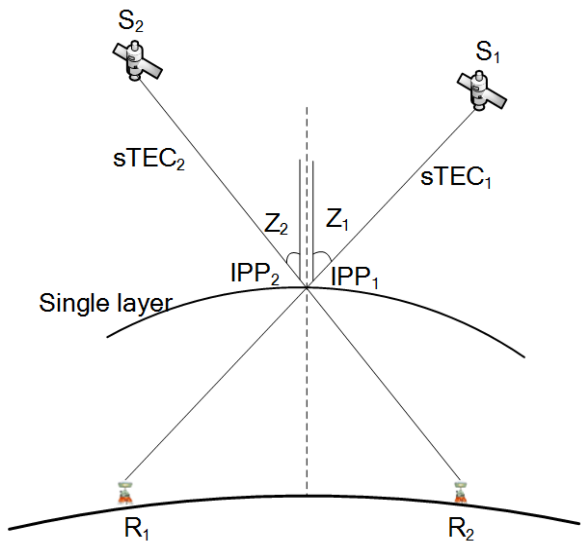
2.1. The CPP Method
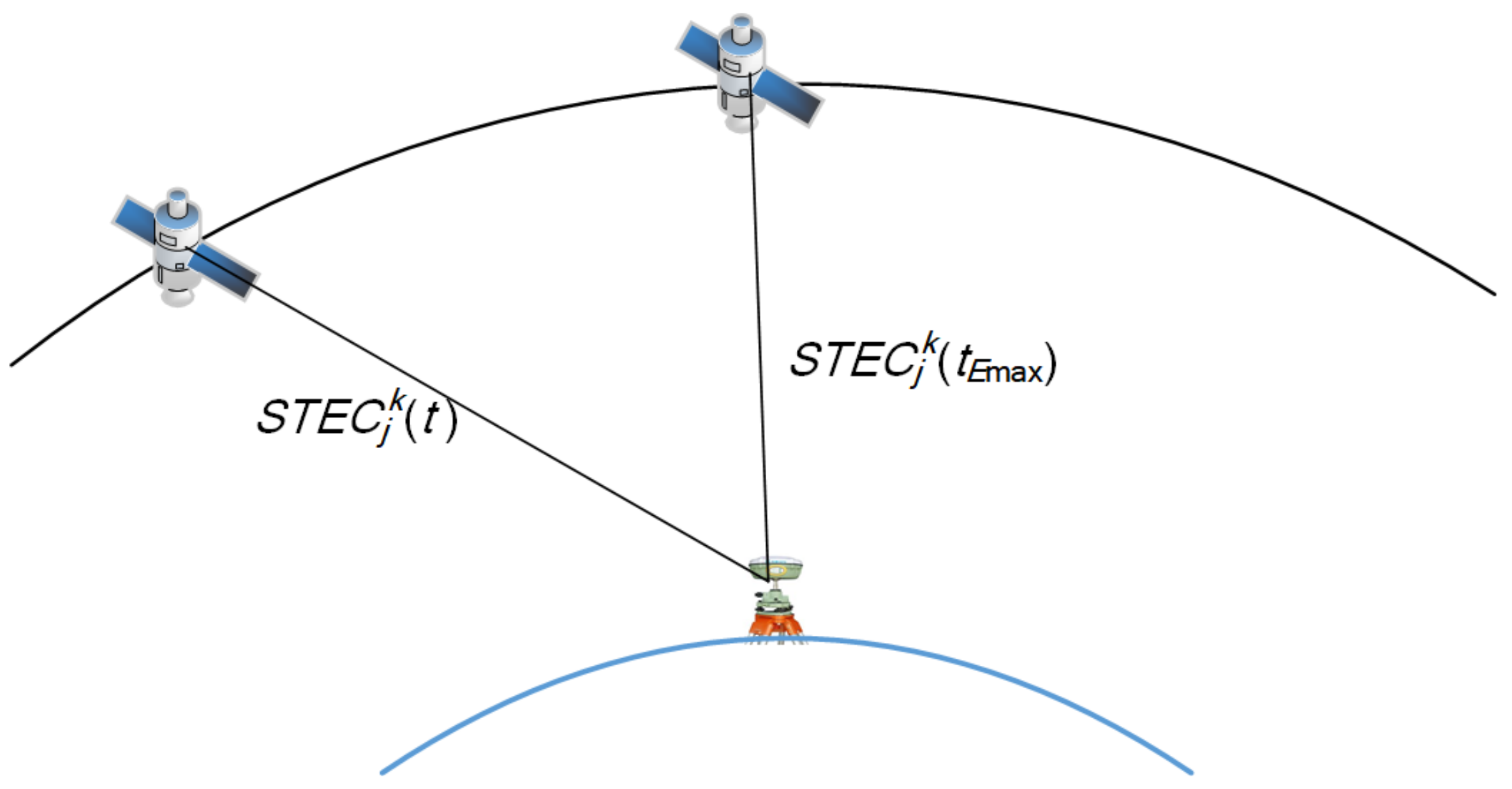
2.2. The dG-TLIH Method
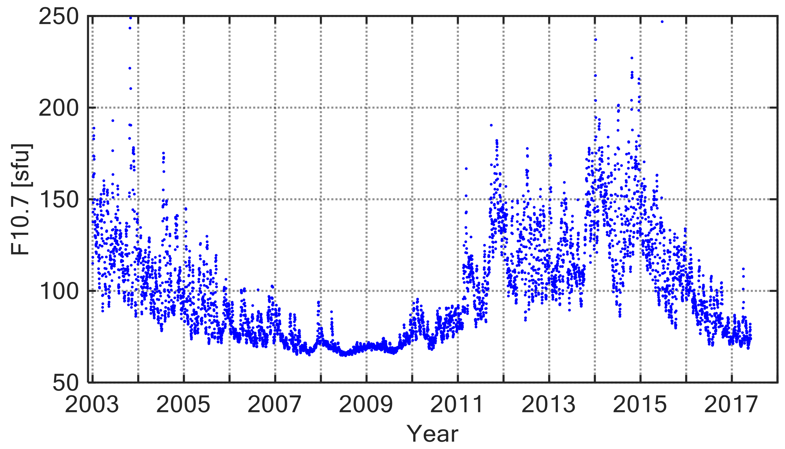
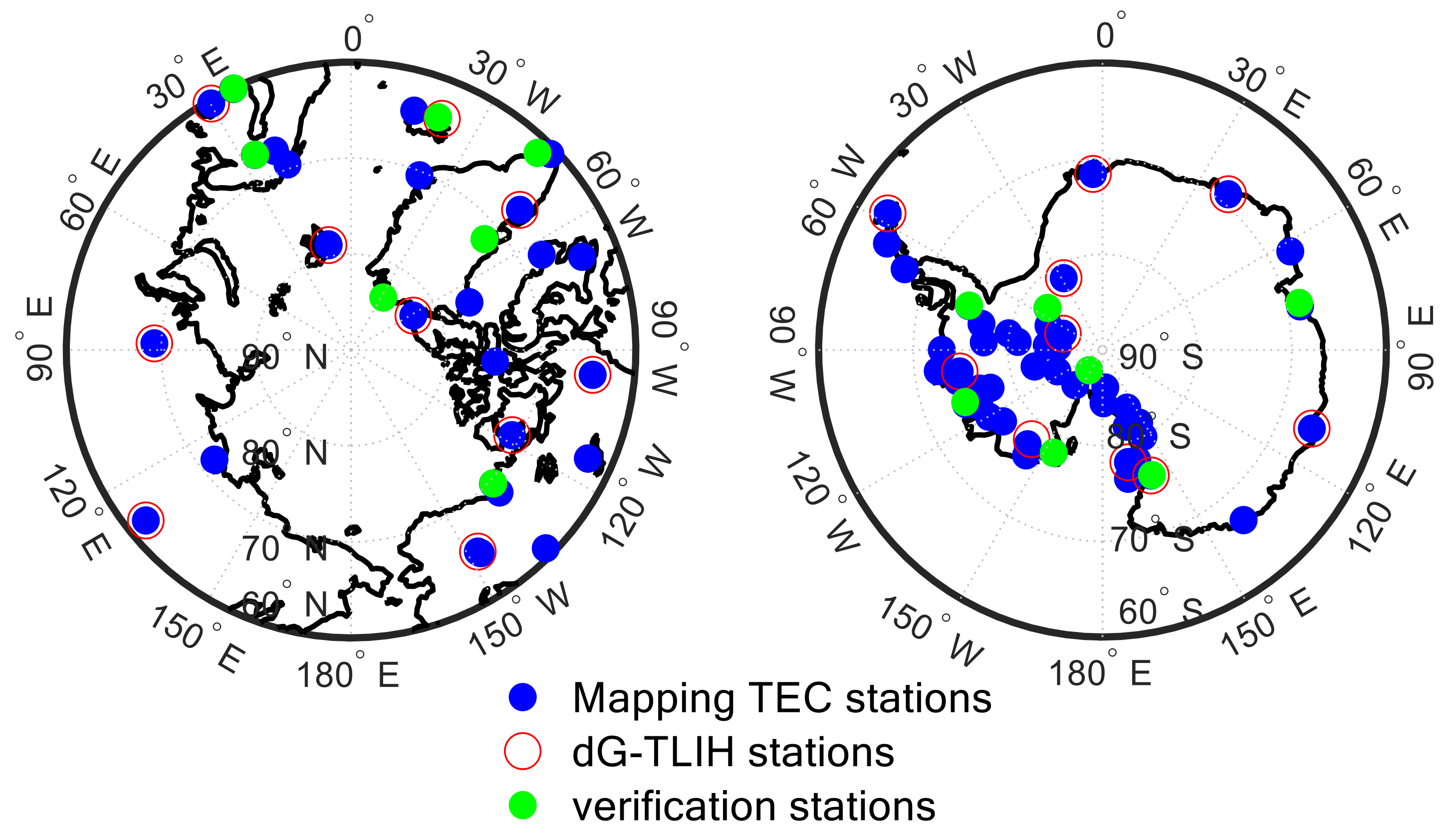
2.3. Observation Data
3. Results and Discussion
3.1. Optimal TLIH Determination Using CPP Method
3.2. Optimal TLIH Determination Using dG-TLIH Method
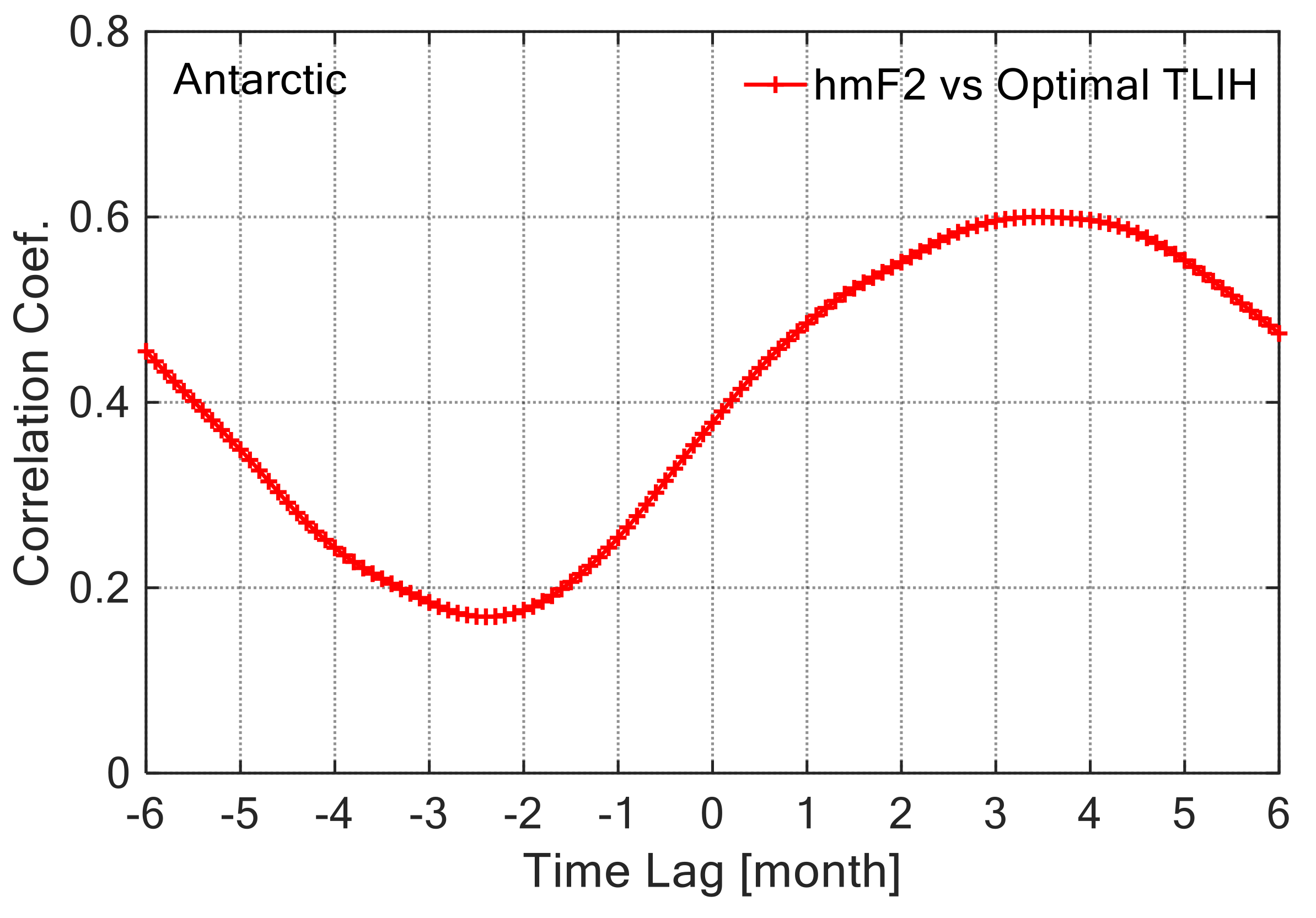
3.3. Relationship between hmF2 and Optimal TLIH
4. Conclusions
Author Contributions
Funding
Institutional Review Board Statement
Informed Consent Statement
Data Availability Statement
Acknowledgments
Conflicts of Interest
References
- Hernández-Pajares, M.; Juan, J.M.; Sanz, J.; Aragón-Àngel, À.; García-Rigo, A.; Salazar, D.; Escudero, M. The ionosphere: Effects, GPS modeling and the benefits for space geodetic techniques. J. Geod. 2011, 85, 887–907. [Google Scholar] [CrossRef]
- Su, K.; Jin, S.; Hoque, M.M. Evaluation of Ionospheric Delay Effects on Multi-GNSS Positioning Performance. Remote Sens. 2019, 11, 171. [Google Scholar] [CrossRef] [Green Version]
- Yuan, Y.; Ou, J. An improvement to ionospheric delay correction for single-frequency GPS users–the APR-I scheme. J. Geod. 2001, 75, 331–336. [Google Scholar] [CrossRef]
- Klobuchar, J.A. Ionospheric time-delay algorithm for single-frequency GPS users. IEEE Trans. Aerosp. Electron. Syst. 1987, 23, 325–331. [Google Scholar] [CrossRef]
- Blanch, J. Using Kriging to Bound Satellite Ranging Errors due to the Ionosphere; Stanford University: Stanford, CA, USA, 2003. [Google Scholar]
- Hernández-Pajares, M.; Roma-Dollase, D.; Krankowski, A.; García-Rigo, A.; Orús-Pérez, R. Methodology and consistency of slant and vertical assessments for ionospheric electron content models. J. Geod. 2017, 91, 1405–1414. [Google Scholar] [CrossRef]
- Schaer, S. Mapping and Predicting the Earth’s Ionosphere Using the Global Positioning System; University of Berne: Berne, Switzerland, 1999. [Google Scholar]
- Brunini, C.; Camilion, E.; Azpilicueta, F. Simulation study of the influence of the ionospheric layer height in the thin layer ionospheric model. J. Geod. 2011, 85, 637–645. [Google Scholar] [CrossRef]
- Hoque, M.M.; Jakowski, N.; Berdermann, J. A new approach for mitigating ionospheric mapping function errors. In Proceedings of the 27th International Technical Meeting of the Satellite Division of the Institute of Navigation (ION GNSS+), Tampa, FL, USA, 8–12 September 2014; pp. 1183–1189. [Google Scholar]
- Zhao, J.; Zhou, C. On the optimal height of ionospheric shell for single-site TEC estimation. GPS Solut. 2018, 22, 48. [Google Scholar] [CrossRef]
- Nava, B.; Radicella, S.; Leitinger, R.; Coïsson, P. Use of total electron content data to analyze ionosphere electron density gradients. Adv. Space Res. 2007, 39, 1292–1297. [Google Scholar] [CrossRef]
- Durmaz, M.; Karslioğlu, M.O. Non-parametric regional VTEC modeling with Multivariate Adaptive Regression B-Splines. Adv. Space Res. 2011, 48, 1523–1530. [Google Scholar] [CrossRef]
- Pullen, S.; Park, Y.S.; Enge, P. Impact and Mitigation of Ionospheric Anomalies on Ground-Based Augmentation of GNSS. Radio Sci. 2009, 44, RS0A21. [Google Scholar] [CrossRef]
- Hernández-Pajares, M.; Juan, J.; Sanz, J. New approaches in global ionospheric determination using ground GPS data. J. Atmos. Solar-Terr. Phys. 1999, 61, 1237–1247. [Google Scholar] [CrossRef]
- Birch, M.J.; Hargreaves, J.K.; Bailey, G.J. On the use of an effective ionospheric height in electron content measurement by GPS reception. Radio Sci. 2002, 37, 1015. [Google Scholar] [CrossRef]
- Jiang, H.; Wang, Z.; An, J.; Liu, J.; Wang, N.; Li, H. Influence of spatial gradients on ionospheric mapping using thin layer models. GPS Solut. 2018, 22, 2. [Google Scholar] [CrossRef]
- Li, M.; Yuan, Y.; Zhang, B.; Wang, N.; Li, Z.; Liu, X.; Zhang, X. Determination of the optimized single-layer ionospheric height for electron content measurements over China. J. Geod. 2018, 92, 169–183. [Google Scholar] [CrossRef]
- Li, Z.; Yuan, Y.; Wang, N.; Hernandez-Pajares, M.; Huo, X. SHPTS: Towards a new method for generating precise global ionospheric TEC map based on spherical harmonic and generalized trigonometric series functions. J. Geod. 2015, 89, 331–345. [Google Scholar] [CrossRef]
- Krankowski, A.; Shagimuratov, I.I.; Ephishov, I.I.; Krypiak-Gregorczyk, A.; Yakimova, G. The occurrence of the mid-latitude ionospheric trough in GPS-TEC measurements. Adv. Space Res. 2009, 43, 1721–1731. [Google Scholar] [CrossRef]
- Hernández-Pajares, M.; Juan, J.M.; Sanz, J.; Orus, R.; Garcia-Rigo, A.; Feltens, J.; Komjathy, A.; Schaer, S.C.; Krankowski, A. The IGS VTEC maps: A reliable source of ionospheric information since 1998. J. Geod. 2009, 83, 263–275. [Google Scholar] [CrossRef]
- Mannucci, A.J.; Wilson, B.D.; Yuan, D.N.; Ho, C.H.; Lindqwister, U.J.; Runge, T.F. A global mapping technique for GPS-derived ionospheric total electron content measurements. Radio Sci. 1998, 33, 565–582. [Google Scholar] [CrossRef]
- Jiang, H.; Liu, J.; Wang, Z.; An, J.; Ou, J.; Liu, S.; Wang, N. Assessment of spatial and temporal TEC variations derived from ionospheric models over the polar regions. J. Geod. 2019, 93, 455–471. [Google Scholar] [CrossRef]
- Wen, J.; Wan, W.; Ding, F.; Le, X.; Yu, C.; Liu, L. Experimental observation and statistical analysis of the vertical TEC mapping function. Chin. J. Geophys. 2010, 53, 22–29. [Google Scholar]
- Xiang, Y.; Gao, Y. An Enhanced Mapping Function with Ionospheric Varying Height. Remote Sens. 2019, 11, 1497. [Google Scholar] [CrossRef] [Green Version]
- Kamide, Y.; Baumjohann, W. Magnetosphere-Ionosphere Coupling. J. Geophys. Res. Space Phys. 1979, 84, 7239–7246. [Google Scholar]
- Liu, J.; Chen, R.; An, J.; Wang, Z.; Hyyppa, J. Spherical cap harmonic analysis of the Arctic ionospheric TEC for one solar cycle. J. Geophys. Res. Space Phys. 2014, 119, 601–619. [Google Scholar] [CrossRef]
- Skone, S.H. Wide Area Ionosphere Grid Modelling in the Auroral Region; University of Calgary: Calgary, AB, Canada, 1998. [Google Scholar]
- Xi, H.; Jiang, H.; An, J.; Wang, Z.; Xu, X.; Yan, H.; Feng, C. Spatial and Temporal Variations of Polar Ionospheric Total Electron Content over Nearly Thirteen Years. Sensors 2020, 20, 540. [Google Scholar] [CrossRef] [Green Version]
- Coley, W.R.; Heelis, R.A. Seasonal and universal time distribution of patches in the northern and southern polar caps. J. Geophys. Res. 1998, 103, 29229–29237. [Google Scholar] [CrossRef]
- Hernández-Pajares, M.; Lyu, H.; Aragón-Ngel, N.; Monte-Moreno, E.; Liu, J.; An, J.; Jiang, H. Polar Electron Content from GPS Data-Based Global Ionospheric Maps: Assessment, Case Studies, and Climatology. J. Geophys. Res. Space Phys. 2020, 125, e2019JA027677. [Google Scholar] [CrossRef]
- Dach, R.; Brockmann, E.; Schaer, S.; Beutler, G.; Meindl, M.; Prange, L.; Bock, H.; Jäggi, A.; Ostini, L. GNSS processing at CODE: Status report. J. Geod. 2009, 83, 353–365. [Google Scholar] [CrossRef] [Green Version]
- Yuan, Y.; Ou, J. A generalized trigonometric series function model for determining ionospheric delay. Prog. Nat. Sci. 2004, 14, 1010–1014. [Google Scholar] [CrossRef]
- Arikan, F.; Erol, C.; Arikan, O. Regularized estimation of vertical total electron content from Global Positioning System data. J. Geophys. Res. 2003, 108, 1469. [Google Scholar] [CrossRef]
- Lunt, N.; Kersley, L.; Bishop, G.J.; Mazzella, A.J.; Bailey, G.J. The effect of the protonosphere on the estimation of GPS total electron content: Validation using model simulations. Radio Sci. 1999, 34, 1261–1271. [Google Scholar] [CrossRef]


| Region | Year | Month | |||
|---|---|---|---|---|---|
| March | June | September | December | ||
| Antarctic | 2009 | (448, 0.08) | (386, 0.16) | (322, 0.06) | (392, 0.02) |
| 2016 | (492, 0.03) | (460, 0.02) | (454, 0.03) | (456, 0.03) | |
| 2014 | (476, 0.02) | (506, 0.04) | (460, 0.02) | (446, 0.01) | |
| Arctic | 2009 | (424, 0.02) | (342, 0.02) | (300, 0.06) | (322, 0.05) |
| 2016 | (466, 0.03) | (414, 0.02) | (410, 0.02) | (412, 0.02) | |
| 2014 | (480, 0.03) | (452, 0.02) | (428, 0.02) | (460, 0.01) | |
| Time | F10.7 (sfu) | Optimal TLIH (km) | |
|---|---|---|---|
| Antarctic | Arctic | ||
| DOY 046, 2014 | 162.1 | 464 | 508 |
| DOY 127, 2014 | 145.9 | 504 | 466 |
| DOY 136, 2017 | 71.9 | 328 | 376 |
| Region | Time | TLIH (km) | Bias (TECU) | RMS (TECU) |
|---|---|---|---|---|
| Antarctic | DOY 046, 2014 | 350 | 5.14 | 7.91 |
| 450 | 2.48 | 5.94 | ||
| 464 | 2.14 | 5.80 | ||
| DOY 127, 2014 | 350 | 1.52 | 3.98 | |
| 450 | 1.09 | 3.75 | ||
| 504 | 0.91 | 3.73 | ||
| DOY 136, 2017 | 350 | 0.36 | 1.64 | |
| 450 | 0.41 | 1.66 | ||
| 328 | 0.35 | 1.64 | ||
| Arctic | DOY 046, 2014 | 350 | 2.90 | 5.51 |
| 450 | 1.81 | 4.96 | ||
| 508 | 1.35 | 4.50 | ||
| DOY 127, 2014 | 350 | 3.41 | 4.66 | |
| 450 | 1.59 | 3.22 | ||
| 466 | 1.36 | 3.12 | ||
| DOY 136, 2017 | 350 | 0.54 | 1.96 | |
| 450 | 0.53 | 1.82 | ||
| 376 | 0.49 | 1.80 |
Publisher’s Note: MDPI stays neutral with regard to jurisdictional claims in published maps and institutional affiliations. |
© 2021 by the authors. Licensee MDPI, Basel, Switzerland. This article is an open access article distributed under the terms and conditions of the Creative Commons Attribution (CC BY) license (https://creativecommons.org/licenses/by/4.0/).
Share and Cite
Jiang, H.; Jin, S.; Hernández-Pajares, M.; Xi, H.; An, J.; Wang, Z.; Xu, X.; Yan, H. A New Method to Determine the Optimal Thin Layer Ionospheric Height and Its Application in the Polar Regions. Remote Sens. 2021, 13, 2458. https://0-doi-org.brum.beds.ac.uk/10.3390/rs13132458
Jiang H, Jin S, Hernández-Pajares M, Xi H, An J, Wang Z, Xu X, Yan H. A New Method to Determine the Optimal Thin Layer Ionospheric Height and Its Application in the Polar Regions. Remote Sensing. 2021; 13(13):2458. https://0-doi-org.brum.beds.ac.uk/10.3390/rs13132458
Chicago/Turabian StyleJiang, Hu, Shuanggen Jin, Manuel Hernández-Pajares, Hui Xi, Jiachun An, Zemin Wang, Xueyong Xu, and Houxuan Yan. 2021. "A New Method to Determine the Optimal Thin Layer Ionospheric Height and Its Application in the Polar Regions" Remote Sensing 13, no. 13: 2458. https://0-doi-org.brum.beds.ac.uk/10.3390/rs13132458