
Cloud-Top Height Comparison from Multi-Satellite Sensors and Ground-Based Cloud Radar over SACOL Site


Key Laboratory for Semi-Arid Climate Change of the Ministry of Education and College of Atmospheric Sciences, Lanzhou University, Lanzhou 730000, China
*
Author to whom correspondence should be addressed.
Remote Sens. 2021, 13(14), 2715; https://0-doi-org.brum.beds.ac.uk/10.3390/rs13142715
Submission received: 6 May 2021
/
Revised: 28 June 2021
/
Accepted: 1 July 2021
/
Published: 9 July 2021
(This article belongs to the Special Issue Aerosol and Cloud Properties Retrieval by Satellite Sensors)
Abstract
:Cloud-top heights (CTH), as one of the representative variables reflecting cloud macro-physical properties, affect the Earth–atmosphere system through radiation budget, water cycle, and atmospheric circulation. This study compares the CTH from passive- and active-spaceborne sensors with ground-based Ka-band zenith radar (KAZR) observations at the Semi-Arid Climate and Environment Observatory of Lanzhou University (SACOL) site for the period 2013–2019. A series of fundamental statistics on cloud probability in different limited time and areas at the SACOL site reveals that there is an optimal agreement for both cloud frequency and fraction derived from space and surface observations in a 0.5° × 0.5° box area and a 40-min time window. Based on the result, several facets of cloud fraction (CF), cloud overlapping, seasonal variation, and cloud geometrical depth (CGD) are investigated to evaluate the CTH retrieval accuracy of different observing sensors. Analysis shows that the CTH differences between multi-satellite sensors and KAZR decrease with increasing CF and CGD, significantly for passive satellite sensors in non-overlapping clouds. Regarding passive satellite sensors, e.g., Moderate Resolution Imaging Spectroradiometer (MODIS) on Terra and Aqua, the Multi-angle Imaging SpectroRadiometer (MISR) on Terra, and the Advanced Himawari Imager on Himawari-8 (HW8), a greater CTH frequency difference exists between the upper and lower altitude range, and they retrieve lower CTH than KAZR on average. The CTH accuracy of HW8 and MISR are susceptible to inhomogeneous clouds, which can be reduced by controlling the increase of CF. Besides, the CTH from active satellite sensors, e.g., Cloud Profiling Radar (CPR) on CloudSat, and Cloud-Aerosol Lidar with Orthogonal Polarization (CALIOP) onboard Cloud-Aerosol Lidar and Infrared Pathfinder Satellite Observation (CALIPSO), agree well with KAZR and are less affected by seasonal variation and inhomogeneous clouds. Only CALIPSO CTH is higher than KAZR CTH, mainly caused by the low-thin clouds, typically in overlapping clouds.
1. Introduction
Clouds, covering approximately two-thirds of the globe, play an important role in radiative energy balance, hydrological cycle, atmospheric circulation, and thus climate change [1,2,3,4,5]. Clouds can reflect solar radiation to space, inducing a cooling albedo effect and trapping the terrestrial radiation, causing a warming greenhouse effect [6,7,8]. Cloud-top heights (CTH) are the highest altitude of the visible part of cloud, which vary with cloud type and can largely influence the cloud radiative effects [9,10,11,12]. For example, high-level cirrus clouds usually have positive forcing due to the large temperature difference between the cloud top and the earth surface that prevents the terrestrial longwave radiation from escaping to space [13,14,15]. In contrast, low-altitude clouds with cloud top temperatures close to the ground environment generally lead to a weak greenhouse effect [16,17,18]. In addition, the radiative cooling at the cloud top and the warming at the cloud base may enlarge the vertical temperature gradient and consequently intensify the turbulence, hence the cloud top does impact the atmospheric stability and can be used to assess the extent of convection development [19,20,21]. CTH also reflects the vertical structure of cloud water content [22], which determines the redistribution of water vapor.
Despite the many related research studies on CTH that have been conducted, accurate representation of CTH in weather and climate models is still one of the great challenges [22,23]. For example, Wang and Zhang [24] show that the simulated tropical convective CTH by the Community Atmosphere Model is 2 km lower on average than satellite measurements. Therefore, the reliable CTH observation is still an essential reference to evaluate cloud simulation and reduce uncertainties in models, especially for the arid and semi-arid regions, which are quite sensitive to climate change and have various cloud types, which in turn may largely affect the climate radiative feedback [25,26,27]. The surface over these regions is relatively bright, and the cloud formation and evolution are also subjected to these complex surface conditions that may affect the accuracy of cloud height from different satellite sensors and retrieval methods. The Semi-Arid Climate and Environment Observatory of Lanzhou University (SACOL) site (35.946°N, 104.137°E; 1965.8 m) is located in the Loess Plateau, the largest semi-arid region of China [26]. A new generation of ground-based Ka-band zenith radar (KAZR, with outstanding cloud penetration capability [28,29,30,31,32,33]) has been continuously operated over the SACOL site since August 2013, which provide a good opportunity to validate and understand the accuracy of multi-satellite cloud-top detections over this region [32].
Previous research analyzing the CTH comparisons has widely utilized spaceborne active/passive sensors with quite different CTH retrieval methods. For instance, the Moderate Resolution Imaging Spectroradiometer (MODIS) onboard polar-orbiting satellites Terra and Aqua combines CO2-slicing and infrared window technologies to determine CTH [34,35]. The Advanced Himawari Imager (AHI) carried by the Himawari-8 (HW8) geostationary satellite derives CTH based on the observation in the visible and infrared bands, thus CTH is only provided during daytime [36,37,38], while the Multi-angle Imaging SpectroRadiometer (MISR) on Terra obtains CTH via a geometrical method named stereo-imaging technique [39,40]. Active instruments such as the Cloud Profiling Radar (CPR) onboard the CloudSat satellite and Cloud-Aerosol Lidar with Orthogonal Polarization (CALIOP) onboard the Cloud-Aerosol Lidar and Infrared Pathfinder Satellite Observation (CALIPSO) satellite directly acquire CTH by measuring the backscattered signal of cloud particles [22,41,42,43]. These satellite observations can obtain global CTH distribution; however, each of them also have some limitations. For example, active spaceborne instruments normally have narrow observing trajectories [9]; passive satellite sensors are usually susceptible to multilayer clouds [18,35,44] and usually have larger discrepancies in low-level clouds than high-level clouds [45,46]. Therefore, using high-quality ground-based observation to compare with satellite measurements is crucial to understand the discrepancies of CTH for the different retrieval methods and instrument sensitivities. Ground-based millimeter-wavelength cloud radar (KAZR) in this study is a powerful instrument that is sensitive to cloud droplets and can detect cloud vertical structure with a high temporal and vertical resolution, as well as long-term continuous observations [47].
CTH comparison from different sensors has been conducted over many places around the world, showing that there may be a significant temporal and spatial influence. Naud et al. [48,49,50] compared MODIS and MISR CTH with lidar and radar measurements over America, England, and France. They found a small difference of 0.1–0.4 km between lidar and MISR for the thin low-level cloud with no upper cloud, and the differences between MODIS and ground-based radar are within 1 km for mid-/high- level clouds and reach nearly 3 km for low-level clouds overlapped with upper clouds. Kim et al. [7] made intercomparisons of CTH among CALIPSO, CloudSat, and ground lidar in South Korea, and found CALIPSO CTH agrees well with CloudSat for thick tropospheric clouds but detects higher CTH for high-level thin clouds, which are more reliable. Firstly, we systematically investigate the CTH comparison between multiple spaceborne observations (i.e., Terra/MODIS, Aqua/MODIS, Terra/MISR, CloudSat/CPR, CALIPSO/CALIOP, and HW8/AHI, commonly used in previous studies) and KAZR over SACOL site. This paper is organized as follows: Section 2 introduces the data product and the methodology. Section 3 presents the results for non-overlapping clouds, overlapping clouds, and all clouds. The conclusions are summarized in Section 4.
2. Data and Methods
2.1. Data
Nearly 7-year observations of MODIS/Terra, MODIS/Aqua, MISR, and CALIPSO (August 2013 to December 2019), as well as more than 4-year measurements of HW8 (July 2015 to December 2019) and CloudSat (August 2013 to December 2017), are used in this study. The synchronized ground-based KAZR observations from August 2013 to December 2019 are also involved in the comparison with satellite observations. Data information is presented in Table 1. The CTH of passive satellite sensors is directly provided from each dataset, i.e., Level-2 MODIS data (MOD06/MYD06), MISR Level 2TC Cloud Products (MIL2TCSP), and Level 2 Cloud Property of HW8 (L2CLP010). The CTH of active satellite sensors is obtained from the cloud mask Products of Level 2 GEOPROF for CloudSat (2B_GEOPRROF) and Level 2 Vertical Feature Mask for CALIPSO (VFM). KAZR CTH is the highest altitude of cloud mask in cloud vertical profiles, and the cloud mask is derived from an improved hydrometeor detection method [32], with clutter being removed by a Bayesian classifier [31]. Furthermore, for passive satellite sensors, the MODIS and HW8 CTH retrieval accuracy depend on the cloud depth, and the lower CTH accuracy mainly occurs on the retrieval of thin cloud with lower cloud depth [22,51]. The CTH accuracy of MISR strongly depends on the brightness and contrast of the clouds between different observing views, and it tends to detect lower thick clouds rather than higher thin clouds in multi-layer conditions [35,45]. The active sensors, i.e., CloudSat and CALIPSO, detect CTH by measuring the reflectivity of cloud top particles, and their CTH accuracy is determined by the size of cloud top particles [52]. In general, the CTH accuracy of CloudSat is lower for cloud tops with small particles, and that of CALIPSO is lower for cloud tops with large particles. The CTH provided by MOD06/MYD06, MIL2TCSP, and L2CLP010 are with resolutions of 5 × 5 km, 1.1 × 1.1 km, 5 × 5 km, respectively. The horizontal and vertical resolutions of 2B_GEOPRROF are 1.3 × 1.7 km and 240 m, and the resolutions are 30 m (60 m) vertically and 333 m (1000 m) horizontally for VFM below (above) 8.2 km. The KAZR observation is continuous, with a time resolution of 4.27 s and a vertical resolution of 30 m, thus it is used as an etalon in this study. Specifically, KAZR is a zenith-pointing radar operating at 35 GHz frequency, with a peak power of 2.2 kW and two pulse mode of “chirp” and “burst”. KAZR provides the vertical profile from the cloud detection algorithm proposed by Ge et al. [32], in which a new noise reduction scheme was developed to enhance the contrast between noise and signal and distinguish more clouds through the reduction of the noise distribution to a narrow range. To reduce the terrestrial clutter contaminant on cloud detection and maintain consistency of the satellites–KAZR comparison, all CTH used in paper is the altitude of the cloud top above mean sea level, and only cloud tops above the minimum detection height of KAZR (i.e., 869 m above ground altitude) are considered.
2.2. Cloud Layer Category
Cloud layer overlap can interfere with the CTH determination and increase the uncertainty in the CTH comparisons; thus, it is necessary to classify cloud overlap scenarios before comparisons. Because all spaceborne sensors involved in this study possess different retrieval methods and operational orbits, we utilize ground observation of KAZR to characterize cloud vertical structure during each satellite observation. Based on previous experience, the KAZR vertical profiles with clouds are divided into single-layer and multi-layer [59,60]. If KAZR detects more than 80% of single-layer profiles within a certain period, the observed cloud is considered as a non-overlapping cloud (e.g., Figure 1a), which contains both individual single-layer cloud and separate single-layer clouds without vertical overlap. The remains are considered as overlapping clouds (e.g., Figure 1b) with more cloud heterogeneity, and may affect satellite’s accuracy of cloud tops especially for passive sensors. Figure 1c presents that the percentage of non-overlapping and overlapping clouds varies slightly when the temporal resolution is within different limited time (from 10 to 120 min with an interval of 10 min). In addition, the autocorrelation of KAZR CTHs with several time intervals less than 120 min are also calculated, explaining the stable temporal variability of clouds over the SACOL site. The limited time of KAZR suitable for all satellite instruments is defined as the window time for CTH comparison, which will be discussed in the next section.
2.3. Time-Space Matching Procedure
Since KAZR detects cloud vertical structure at a single point, while satellites cover a certain area along the flying track, a proper time interval and a space area for comparison between space- and ground-based observing platforms must be determined. The fundamental statistics about average cloud fraction (ACF), cloud frequency (CFR), and the integration of ACF and CFR (i.e., average cloud fraction × cloud frequency, ACFR), which represent the probability of cloud within a certain time and area [2,61], were conducted carefully in Figure 2. Here, the satellite cloud fraction (CF) is the proportion of the number of cloudy sub-satellite pixels to the number of all sub-satellite pixels in a box area central at the SACOL site (from 0.25° × 0.25° to 1.50° × 1.50°); the KAZR CF is the ratio of the cloudy profile to all profiles within the window time (from 10 min to 120 min). ACF refers to the average satellite CF or the average KAZR CF. CFR represents the cloud frequency of occurrence, and the occurrence is 0 when CF = 0 and 1 when CF > 0 in each available observation from satellite or KAZR.
The ACF maximizes at 0.25° × 0.25° for all spaceborne sensors except CALIPSO and is shown in Figure 2a. The CFR of all passive satellite sensors gradually increases with the increase in the area in Figure 2b. Note that a bump exists for CALIPSO (Figure 2a–c) at 1.25° × 1.25°, and this is because there are two additional descending tracks counted when the area greater than 1.00° × 1.00° in which only one ascending track is involved. Relative to other sizes, 0.50° × 0.50° implies that the differences in both CF distribution and occurrence are minimal for most satellite instruments. In particular, the ACF and CFR of MODIS (Terra and Aqua), HW8, and CALIPSO vary slowly from 0.50° × 0.50°, and the maximum ACFR for most satellites also occurs at 0.50° × 0.50°. We analyzed the changes of KAZR ACF, CFR, and ACFR corresponding to each satellite instrument in different windows of time to determine the appropriate period (Figure 2d–f). We found that KAZR ACFR for CloudSat and CALIPSO significantly increases as the window time does, varying from 20 min to 70 min. Besides, in Figure 2g,h, the ACF differences are minimized at 20 min for CALIPSO, 40 min for CloudSat, and 100 min for MODIS Terra. The ACF difference is smaller than 10% for MODIS (Terra and Aqua), CloudSat, and CALIPSO when the window time exceeds 40 min. Meanwhile, the minimum difference of CFR between CALIPSO and KAZR appears at 40 min. Thus, we select 40 min as the optimal window of time for multi-satellite sensors [61].
3. Results
3.1. Comparison for Non-Overlapping Clouds
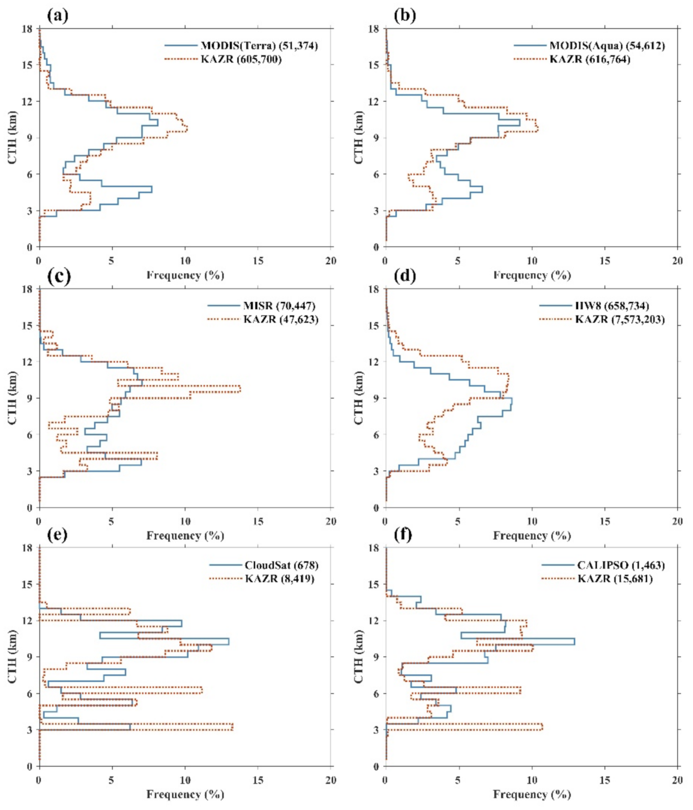
Before directly comparing the CTH from the different instruments, we first examine the vertical frequency distribution (Figure 3) and the seasonal variations (Figure 4) of CTH using the original observation samples (marked in the bracket of each panel) within the selected 0.5° × 0.5° box and 40 min interval for the non-overlapping clouds, which represent the best inter-comparison scenario by avoiding the complexity of multi-layer cloud conditions. Figure 3 shows that nearly all instruments capture the bimodal structure of CTH, peaking close to 10 km and 5 km, except HW8 only has one peak near 9 km. The CTH obtained from most spaceborne sensors presents better agreement with KAZR for the high-level cloud top above 6 km than the low-level altitude below 6 km. In Figure 3a–c, the frequencies of CTH above 6 km from MODIS and MISR are smaller than that from KAZR, while they are opposite below 6 km. The distribution differences of passive satellite sensors and KAZR CTH show that KAZR may have better sensitivity to high-level clouds, or low-level dispersed clouds are easily observed by satellite sensors with broad footprints. Unlike passive satellite sensors, the CTH curves from active satellite sensors are less smooth due to the relatively small, matched samples. As shown in Figure 3e,f, the CTH frequencies of CloudSat and CALIPSO are very consistent with KAZR especially for the cloud top above 9 km. The frequencies of active satellite sensors are underestimated compared with that of KAZR for the cloud top below 6 km, which is different from the results for passive satellite sensors in Figure 3a–c. This is not surprising, since the atmosphere-induced attenuation can lead to a weaker sensitivity of spaceborne sensors than ground-based radar to detect low-level CTH [62,63].
The seasonal distributions of CTH in Figure 4 depict that the differences between passive satellite sensors and KAZR-derived CTH are comparatively larger than that of active satellite sensors. For example, in winter, a MODIS-derived CTH higher than 6 km accounts for 56% of the total cloud samples, while this proportion for KAZR is about 82%, suggesting that the distribution differences in Figure 3a,b are dominated by clouds in winter. The vertical CTH distribution of HW8 is also quite different from that of KAZR in winter (Figure 4(d4)). Previous studies have shown that high-latitude cirrus clouds occur more often during the cold season over the SACOL site [30,33]. These cirrus clouds may not be well identified by the CO2-slicing technology used by MODIS and HW8, which is susceptible to the albedo of snow and ice surface [22,46,64]. The CTH frequency distribution from MISR exhibits a good consistency with KAZR observation in winter and autumn, but significant differences appear in summer (in Figure 4(c2)) when MISR CTH distributes at a lower altitude than KAZR, primarily from the high and thin clouds caused by the high surface temperature [46,50,65]. Active satellite sensors show good agreement with KAZR especially for high clouds in all seasons. The underestimations of CTH occurrence for CloudSat and CALIPSO compared with KAZR in Figure 3e,f mainly occur in summer and winter, which may be related to the strong attenuation by thick clouds or precipitation during these seasons.
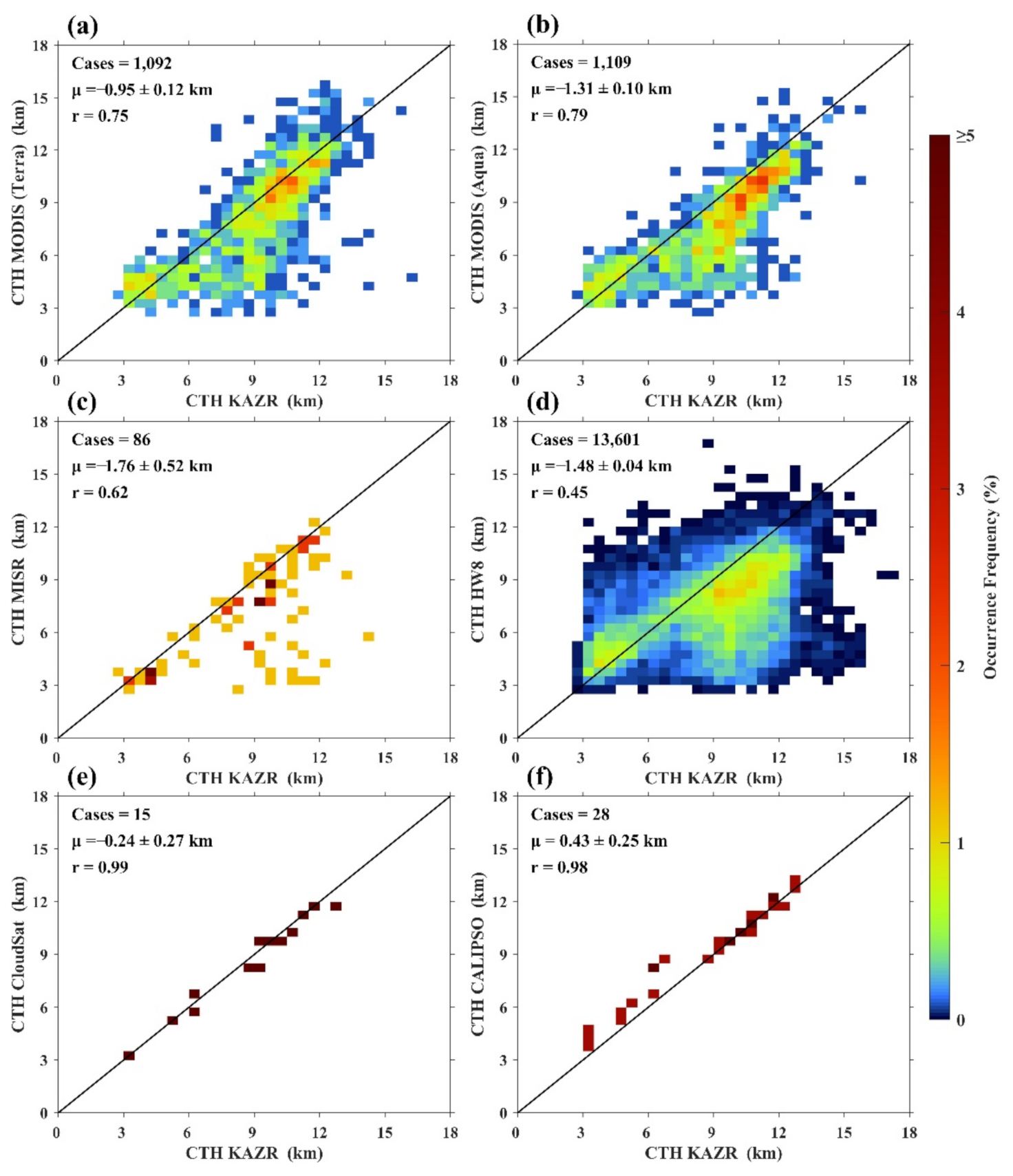
To quantify the CTH difference for space- and ground-based observations, we calculate the average CTH retrieved by satellites and from their respective matched KAZR detections for each cloudy case as shown in Figure 5. It is clear that the CTH deviation is more obvious for passive satellite sensors (Figure 5a–d), and their CTH mainly distributes below the 1:1 line, whereas the CTH from active satellite sensors concentrates near the 1:1 line. For passive satellite sensors, satellites underestimate the CTH compared to KAZR for most cases, with 78–86% of differences less than 3 km. The mean CTH difference between MODIS Terra and KAZR (−0.95 km) is smaller than that between MODIS Aqua and KAZR (−1.31 km), because thin, high clouds appear more frequently in Aqua’s field of view, which is caused by the afternoon convection [1,46]. MISR and HW8 CTH are, on average, lower than KAZR CTH by 1.76 km and 1.48 km, respectively. These large differences are mainly from the cases where the cloud tops above 9 km derived from KAZR are identified as cloud tops below 6 km by satellites (Figure 5c,d), which may probably be attributed to cloud inhomogeneity and surface condition [65]. For active satellite sensors, the CTH difference between CloudSat and KAZR is ranging from −1.24 km to 0.77 km, with a mean value of −0.24 km. The CTH differences for all CALIPSO-KAZR cases are from −0.49 km to 1.89 km, and the average value is 0.43 km, meaning that CALIPSO-retrieved CTH is higher than KAZR. This is normal because CALIPSO is more sensitive to the small particles at the cloud top than microwave radar [52,66]. In addition, the correlation coefficients of CTH between active satellite sensors and KAZR are significantly larger than that between passive satellite sensors and KAZR, implying that active satellite sensors may obtain the cloud top more accurately.
The spatial inhomogeneity of cloud properties can affect the CTH comparisons [67]. In previous studies, cloud inhomogeneity can be assumed by the CF variation in observations [60,68]. Here, to understand its effects on the comparisons, we analyze the variations of three main factors (i.e., case frequency, correlation coefficient, and mean CTH difference) as a function of CF in Figure 6. Overall, passive satellite sensors are more susceptive to CF variation than active satellite sensors, and dramatic influences exist, especially for MISR and HW8. As CF increases, the cases of MISR and HW8 decrease more intensely than other instruments, and there are obvious improvements in the correlation coefficient and the CTH differences. When the CF increases from 0% to 100%, the CTH correlation coefficient between MISR (HW8) and KAZR increases from 0.62 to 1.00 (from 0.45 to 0.74). The mean CTH difference between MISR (HW8) and KAZR varies over a large range. The minimal difference is 0 km (−0.69 km) when CF is at about 85% (95%). These results demonstrate that cloud inhomogeneity can induce large CTH differences for MISR and HW8 (presented in Figure 4). Furthermore, as CF increases, the CTH correlation coefficient between MODIS and KAZR barely varies, which is similar to that from active satellite sensors. However, the mean CTH difference between MODIS and KAZR decreases slightly, and the minimal difference for Terra and Aqua is −0.35 km and −0.87 km, respectively, when CF is 100%. Comparing this with passive satellite sensors, active satellite sensors are less influenced by CF changes. In particular, the correlation coefficient and the mean CTH differences remain almost constant, which is similar to the results illustrated in Figure 5e,f. This indicates that the inversion capability of CloudSat and CALIPSO on cloud tops is less influenced by inhomogeneity clouds.
3.2. Comparison for Overlapping Clouds
Similar to the CTH comparisons for non-overlapping clouds that reduce the influence of complex cloud structure on cloud top detections, in this section, we begin with illustrating the vertical distributions of CTH derived from different sensors for overlapping clouds as presented in Figure 7. The occurrence frequency of KAZR CTH shows a unimodal structure converging to about 10 km, which differs from the bimodal structure of non-overlapping clouds. Compared to non-overlapping clouds, the difference in CTH distribution between satellite and KAZR is particularly apparent below 6 km, especially for passive satellite sensors. This demonstrates that the complexity of the overlapping clouds strongly affects the ability of cloud top detection for passive satellite sensors. In detail, MODIS onboard Terra and Aqua capture the peak frequency of CTH at high altitudes, but the occurrence frequency of CTH at altitude below 6 km is significantly larger than KAZR. In addition to the reasons mentioned in Section 3.1, when multi-layer clouds simultaneously occur in the same location, the height of upper-level semi-transparent clouds cannot be accurately retrieved by the CO2 method of MODIS [46]. Besides, the location of the strongest infrared emissivity (generally below the upper boundaries of the highest cloud layer) is more likely to be identified by MODIS and HW8 as cloud tops [48,60], which also leads to more low cloud top detections. In Figure 7d, HW8 also has a unimodal distribution, but with a peak of 6–8 km that is lower than the peak of 9 km for non-overlapping clouds (Figure 3d). Furthermore, although MISR and KAZR-derived CTH have good agreement without cloud overlap (Figure 3c), Figure 7c shows that the MISR CTH distributes below 6 km and peaks at around 4 km, which is significantly lower than the peak height of KAZR CTH. Ordinarily, the geometric stereo-imaging technique of MISR is sensitive to the thick clouds with larger contrast between two view directions [45,69]; therefore, the underlying thick clouds are more easily identified as the cloud top than the upper thin clouds. Contrary to the results of passive satellite sensors, Figure 7e,f shows that there are good consistencies in CTH frequency between active satellite sensors and KAZR, though the small number of samples produces obvious sharp curves in the vertical direction. Note that the highest CTH observed by KAZR is higher than CloudSat, but lower than CALIPSO, which again demonstrates that the cloud tops composed of small particles can be more easily detected by CALIPSO, while KAZR has better sensitivity to small cloud droplets than CloudSat.
The seasonal variations of CTH frequency for overlapping clouds are shown in Figure 8. Compared with the distribution of KAZR CTH, the significant differences occur in winter for MODIS and HW8, and summer for MISR, which are similar to the results in Figure 4a–d. However, the height differences of CTH peak frequency between passive satellite sensors and KAZR in overlapping clouds have a seasonal variation. The peak height of CTH for high clouds from MODIS is slightly lower than that from the KAZR, and their distance is about 3 km (Figure 8(a2,b2)). The HW8-retrieved CTH concentrates at the altitude of 6–9 km, which is lower than the peak frequency height of KAZR-retrieved CTH, and the distance reaches up to 6 km (Figure 8(d2)). The peak frequency height of MISR CTH is around 4 km, which is significantly lower than that of KAZR CTH by 9 km (Figure 8(c2)). Therefore, high surface temperature and strong convection in summer have the largest impact on MISR, which follows previous results (Figure 4(c2)). Moreover, for active satellite sensors, the highest CTH above CloudSat and below CALIPSO observed by KAZR presented in Figure 7c–f only occurs in summer (Figure 8(e2,f2)), which also implies that some small cloud particles appear at a high altitude in summer. The vertical distribution of CTH frequency for active satellite sensors is quite similar to that for KAZR in all seasons except winter, when KAZR does not observe the cloud top around 3 km as CloudSat, possibly caused by the broken clouds. Overall, the seasonal difference in vertical CTH frequency between active satellite sensors and KAZR is smaller than that between passive satellite sensors and KAZR.
Figure 9 shows the scatter plot of the CTH difference between satellite and KAZR observations. As shown in Figure 9a–d, the frequency density of satellites is mostly distributed below the 1:1 line, and the high-frequency value is located at high altitudes, demonstrating that overall, passive satellite sensors retrieved CTH lower than KAZR. The CTH derived from MODIS Terra (Aqua) has a negative difference of 1.49 km (1.74 km) on average than that from KAZR, and HW8-retrieved CTH is lower than KAZR CTH by a mean of 1.94 km. The mean CTH difference between MISR and KAZR is −2.46 km, and the high-frequency location of MISR is lower than that of MODIS and HW8. Comparing Figure 9a–d with Figure 3a–d, a significant systematic underestimation of the cloud top for passive satellite sensors appears in the presence of multi-layer clouds. Aside from these explanations proposed for non-overlapping clouds, there are two other possible reasons. One is that the radiative contribution of each cloud layer may influence the CTH comparison, and the low-level clouds-reflected radiation penetrates the upper thin clouds, leading to a higher brightness temperature than the actual cloud top temperature observed by MODIS and HW8 [9]. Another is that the MISR stereo method more easily detects underlying thick clouds with distinct cloud features between different viewing angles, which are frequently found in a low-level altitude [70]. In addition, for active satellite sensors, it can be seen that the CTH detected by CALIPSO and KAZR agrees well (Figure 9e), as the correlation coefficient is 0.87 and the mean CTH difference is also positive (0.26 km), which is similar as that for non-overlapping clouds, suggesting that CALIPSO is susceptible to the cloud tops composed of smaller particles. However, there is less agreement between CTH measured by CloudSat and KAZR than the comparison in non-overlapping cloud (Figure 5e). In Figure 9e, the outlier data with a CTH difference greater than 6 km account for approximately 6% of CloudSat cases, and CALIPSO does not detect them; therefore, it is probably caused by broken clouds. If these cases are removed, the mean CTH difference between CloudSat and KAZR decreases to −1.04 km, and the correlation coefficient increases to 0.91.
Figure 10 shows the variation of the three factors with CF. In Figure 10a, the available analysis cases corresponding to different satellite observations decrease evenly with increasing CF, and the decline is more significant for MISR and HW8. In Figure 10b,c, the agreement between satellites- and KAZR-retrieved CTH is weaker than that from that for non-overlapping clouds (Figure 6b,c), and it is possibly because of the more complex cloud structure and more inhomogeneous clouds in overlapping clouds. When CF increases from 0% to 100%, the correlation coefficient for MODIS Terra (Aqua) varies within 0.68–0.71 (0.73–0.77), and the mean CTH difference between MODIS Terra (Aqua) and KAZR gradually decreases from −1.53 km to −0.88 km (−1.88 km to −1.58 km). The CTH derived from HW8 and KAZR also shows the best agreement at 100% CF, where the correlation coefficient is 0.57 and the mean CTH difference is −1.70 km. However, significant fluctuations are found for MISR, particularly as the correlation coefficient is at maximum (0.55) when CF is greater than 40%, and the mean CTH difference is at minimum (−1.72 km) when CF is greater than 90%. For active satellite sensors, CALIPSO CTH agrees well with KAZR observation. The correlation coefficient ranges from 0.86 and 0.94, and the mean CTH difference is between −0.06 km and 0.26 km, which is close to the results for non-overlapping clouds (Figure 6). Nevertheless, the difference in CTH between CloudSat and KAZR is significantly larger for overlapping clouds, with a relatively smaller correlation of 0.75 and a larger difference of −1.11 km. This is most likely due to the presence of stronger convection in multi-layered clouds compared to single-layer clouds; consequently, the small cloud particles more easily ascend than larger cloud particles. In this case, the sensitivity of CloudSat to the cloud top is weaker than KAZR.
3.3. Comparison for All Clouds
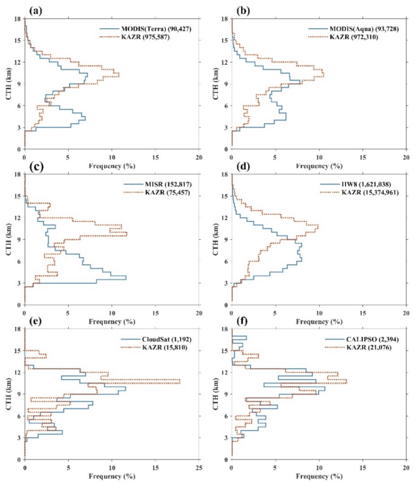
The vertical frequency distributions of KAZR CTH matched with different spaceborne sensors and the frequency difference between satellite and KAZR at each altitude bin are provided in Figure 11a,b for all clouds, including non-overlapping and overlapping clouds. Overall, in Figure 11a, the distributions of KAZR CTH exhibit a unimodal structure, and the obvious crest concentrates slightly above 9 km, which is closer to the distribution of KAZR in overlapping clouds (Figure 7). In Figure 11b, lower frequency differences appear at around 9 km implying better agreement of CTH between satellites and KAZR at this altitude. In particular, the occurrence frequency of CTH from passive satellite sensors is systematically less (more) than that from KAZR at high (low) altitude above (below) approximately 9 km, with a maximum difference of 6%. In comparison, the vertical distribution of CTH frequency differences between active satellite sensors and KAZR exhibit multi-crest structures with smaller amplitudes of about less than 6%. Thus, it demonstrates a better agreement on CTH between active satellite sensors and KAZR. Then, we introduce another important factor, cloud geometrical depth (CGD), which impacts the accuracy of satellite-retrieved CTH, especially for passive satellite sensors. In this section, CGD is the vertical depth of the uppermost cloud layer determined from the KAZR observations matched with each satellite sensor. As illustrated in Figure 11c, the thick clouds with a mean CGD greater than 2 km are mainly distributed at an altitude with CTH higher than 9 km. The maximum peak of the CTH-CGD distribution occurs in the CTH range of 12–13 km for each satellite, with the maximum mean CGD approximately 4 km. This indicates that the thick clouds over the SACOL site frequently exist around the altitude range, possibly as a result of strong convective development. Most satellite sensors can measure thinner clouds in the upper troposphere above 13 km; however, those clouds are rarely detected by CloudSat. Consequently, the negative difference between CloudSat and KAZR CTH is greater in overlapping clouds, probably due to the presence of high-thin clouds with smaller particles. In addition, the average CGD of passive satellite sensors is slightly greater than the median value, and the distribution of active satellite sensors fluctuates more significantly, which can be attributed to the difference in sample amount between passive and active satellite sensors.
Furthermore, to explore the dependence of CTH accuracy on CGD for different satellites, we perform the scatterplot of satellite-derived CTH as a function of KAZR-derived CTH, sorted by the average CGD for each case in Figure 12. For the high-frequency CTH with good agreement along with the 1:1 line in non-overlapping (Figure 5) and overlapping clouds (Figure 9), most are the clouds with CGD ≥ 2 km, again showing that satellites and KAZR-derived CTH are better for thick clouds. For the clouds with CGD < 2 km, the distributions exhibit larger deviation from the 1:1 line, implying that the larger CTH difference between satellites (except CALIPSO) and KAZR for overlapping clouds than that for non-overlapping clouds is due to the presence of thin upper clouds. Quantitatively, the correlation coefficient on CTH between MODIS Terra (Aqua) and KAZR is 0.70 (0.75) for all cases, which varies from 0.74 (0.79) for thick clouds to 0.61 (0.65) for thin clouds. For MISR and KAZR CTH, the correlation coefficient for thick clouds (0.47) is also higher than that for thin clouds (0.37). In addition, CTH detected by active satellite sensors and KAZR agree well, and the correlation coefficient when CGD ≥ 2 km (i.e., 0.92 for CloudSat and 0.93 for CALIPSO) is significantly larger than that when CGD < 2 km (i.e., 0.77 for CloudSat and 0.88 for CALIPSO). However, the agreement between HW8 and KAZR CTH does not become better as CGD thickens, possibly correlating with the inhomogeneous clouds and the surface condition in HW8’s view angle proposed previously.
Figure 13 shows the frequency distribution of the CTH differences between satellites and KAZR for different CGD and when KAZR CTH is above and below 9 km. Overall, except for the CALIPSO-KAZR, most distributions appear negatively skewed, suggesting that the satellite-retrieved CTH is commonly lower than KAZR. In general, the magnitude of the mean CTH difference between satellites and KAZR for thick clouds is smaller than that for thin clouds; nevertheless, the same situation does not occur for MISR and HW8 when CTH is below 9 km, implying a greater influence caused by low-level inhomogeneous clouds. Moreover, for thin clouds, the absolute mean differences between satellites (except CALIPSO) and KAZR-retrieved CTH above 9 km become significantly larger than those below 9 km. Thus, this demonstrates that the large CTH differences between satellites and KAZR are mainly caused by the upper high-thin clouds, as well as the fact that the differences for thick clouds are smaller, which are similar to the findings of Mitra et al. [35]. Specifically, the mean CTH differences between MODIS Terra (Aqua) and KAZR are negative, with the smallest difference of −0.48 km (−0.75 km) for thick clouds when CTH is below 9 km. For CTH below 9 km with different CGD, the CTH derived from MISR and HW8 also have smaller differences than that from KAZR, and the mean difference is −0.88 km and 0.12 km, respectively. Relative to the distribution of passive satellite sensors, the maximum crests of active satellite sensors show narrower width, wherein the mean CTH difference between CloudSat and KAZR is smaller for thick clouds, −0.49 km for CTH above 9 km, and −0.39 km for CTH below 9 km. Besides, compared with KAZR CTH above (below) 9 km, CALIPSO CTH is slightly lower (significantly higher). CALIPSO- and KAZR-retrieved CTH show good agreement when CTH is above 9 km, with the smallest difference of −0.03 km for thick clouds.
4. Discussion and Conclusions
The main objective of this paper is to compare the cloud-top heights (CTH) retrieval capabilities of the currently most widely used passive and active satellite sensors with the ground-based cloud radar (KAZR) located at the SACOL site in the semi-arid region of northwest China. The spatial area of 0.5° × 0.5° centered on the SACOL site and the window time of 40 min centered on the satellite’s passing moment are determined with the possibility of cloud occurrence and cloud fraction variation. To quantify the CTH retrieval accuracy of spaceborne sensors, we investigate the influence of cloud fraction (CF), cloud overlapping, seasonal variation, and cloud geometrical depth (CGD) in CTH comparison.
For the vertical frequency distribution of non-overlapping clouds CTH occurrence, the distributions of satellites (except HW8) and their matched KAZR observations are bimodal structures with peaks at around 5 km and 10 km, respectively. However, for multilayer clouds, the distributions of KAZR CTH corresponding to different satellites are unimodal structures with a peak of around 10 km. Although only smaller numbers of samples for active satellite sensors are selected, they agree well with KAZR-retrieved CTH. Moreover, this phenomenon, where the CTH frequency of satellite is more (less) than that of KAZR at low (high) altitude, is more apparent for passive satellite sensors. There are three possible reasons: (1) Passive satellite sensors cannot easily retrieve the actual heights of semi-transparent clouds appearing in the upper segment of multi-layer clouds; (2) the infrared radiation from each cloud layer penetrating the upper thin clouds leads MODIS and HW8 to observe cloud top with higher brightness temperature; and (3) the underlying thick clouds appearing below the thin clouds are easily observed by MISR. Overall, this suggests that cloud overlap has a greater impact on the passive satellite sensors to detect accurate cloud tops, possibly resulting in cloud tops lower than actual altitude.
Furthermore, for passive sensors, we found that the largest CTH errors exist in summer for MISR and in winter for MODIS and HW8, which are possibly caused by convective clouds and the complex surface albedo conditions, respectively. For active satellite sensors, the seasonal differences are smaller. The highest cloud top observed by CloudSat (CALIPSO) is lower (higher) than that observed by KAZR in summer, which illustrates that CloudSat (CALIPSO) has a weaker (stronger) sensitivity to detect cloud tops with large (small) particles than KAZR.
We quantified the effects of cloud inhomogeneity on the comparison of different platforms through the CF control, which has not been well considered before. In general, there is a smaller difference and a better agreement between satellites and KAZR when the CF is larger. Specifically, the mean CTH difference between passive satellite sensors and KAZR decreases as CF increases, while that between active satellite sensors and KAZR changes less with increasing CF. In general, for non-overlapping (overlapping) clouds with CF greater than 80%, the minimum mean CTH differences between passive satellite sensors and KAZR are −0.35 km (−0.88 km) for MODIS Terra, −0.87 km (−1.58 km) for MODIS Aqua, −0.69 km (−1.70 km) for HW8, and 0 km (−1.72 km) for MISR, respectively. In addition, CloudSat CTH is lower than KAZR CTH by 0.24 km (1.11 km), and CALIPSO CTH is higher than KAZR CTH by 0.43 km (0.26 km), on average. Overall, the CTH difference between satellite sensors and ground-based observations is strongly related to cloud inhomogeneity, which can be reduced by CF increase. The inhomogeneous cloud for non-overlapping clouds is less than that for overlapping clouds, due to the uniform cloud top and simple vertical structure.
Most of satellite-retrieved CTH (except CALIPSO) is lower than KAZR, and the CTH underestimation in overlapping clouds is significantly larger than that in non-overlapping clouds. In particular, the larger CTH error of MODIS Aqua than that of MODIS Terra is mainly from the high-thin clouds caused by strong convection in the local afternoon. Besides, the CTH correlation between active satellite sensors and KAZR is much better than that between passive satellite sensors and KAZR. Compared with KAZR CTH, the CTH overestimation (underestimation) of CALIPSO (CloudSat) in non-overlapping clouds is slightly smaller (significantly larger) than that in overlapping clouds, possibly because of the uppermost high-thin clouds with smaller particles.
To explore the dependence of CTH on cloud thickness, we analyze CGD of the uppermost cloud layer. For all clouds, when CTH is below (above) 13 km, the CGD gradually becomes thicker (thinner) as CTH increases, with the maximum mean CGD of 4 km. In general, CALIPSO detects higher cloud tops than KAZR due to its high sensitivity to small cloud particles, and here we found that the CTH difference is larger for low-thin clouds, which has not been well recognized before. Except for CALIPSO, the mean CTH differences between satellites and KAZR when CTH is below 9 km is smaller than that above 9 km, and the agreement for the thick clouds is better than that for the thin clouds. Therefore, the large differences between satellites (except CALIPSO) and KAZR CTH detections are mainly from the high-thin clouds. Overall, for all satellite sensors, the CGD effect on CTH accuracy is more significant above 9 km than below 9 km, which reflects that the CTH uncertainty of satellite is greater for high-altitude clouds than for low-altitude clouds. This is probably because thicker clouds often coincide with higher cloud tops, while lower cloud tops tend to be accompanied by thinner clouds.
Author Contributions
Conceptualization, J.G. and X.Y.; methodology, X.Y.; software, X.Y.; data collection, X.Y. and X.H.; validation, X.Y., J.G. and X.H.; formal analysis, X.Y.; writing—original draft preparation, X.Y.; writing—review and editing, X.Y., J.G., X.H., M.W. and Z.H. All authors have read and agreed to the published version of the manuscript.
Funding
This work was supported by the National Science Foundation of China (41922032 and 41875028), the National Key R & D Program of China (2016YFC0401003), and the Fundamental Research Funds for the Central Universities (lzujbky-2019-it04).
Institutional Review Board Statement
Not applicable.
Informed Consent Statement
Not applicable.
Data Availability Statement
The data were obtained from NASA Level-1 and Atmosphere Archive & Distribution System Distributed Active Archive Center (MODIS Aqua/Terra, https://ladsweb.modaps.eosdis.nasa.gov/, accessed on 18 July 2020), the NASA Langley Research Center Atmospheric Science Data Center (MISR, https://eosweb.larc.nasa.gov/datapool, accessed on 18 July 2020; CALIPSO, https://eosweb.larc.nasa.gov/project/calipso/calipso_table, accessed on 18 July 2020), the NASA CloudSat data processing center (CloudSat, http://www.cloudsat.cira.colostate.edu/direct-ftp-access, accessed on 18 July 2020), Japan Aerospace Exploration Agency Himawari Monitor and the P-Tree system (Himawari, https://www.eorc.jaxa.jp/ptree/registration_top.html, accessed on 18 July 2020), and the SACOL data archive (KAZR, http://climate.lzu.edu.cn, accessed on 18 July 2020).
Acknowledgments
We thank the MODIS Terra/Aqua, MISR, HW8, CloudSat, CALIPSO, and KAZR science teams for providing excellent and accessible data that made this study possible. We would also like to thank the constructive comments from the editor and two anonymous reviewers to improve the quality of this paper.
Conflicts of Interest
The authors declare no conflict of interest.
References
- King, M.; Platnick, S.; Menzel, W.P.; Ackerman, S.; Hubanks, P.A. Spatial and Temporal Distribution of Clouds Observed by MODIS Onboard the Terra and Aqua Satellites. IEEE Trans. Geosci. Remote. Sens. 2013, 51, 3826–3852. [Google Scholar] [CrossRef]
- Oreopoulos, L.; Norris, P.M. An analysis of cloud overlap at a midlatitude atmospheric observation facility. Atmos. Chem. Phys. Discuss. 2011, 11, 5557–5567. [Google Scholar] [CrossRef] [Green Version]
- Weisz, E.; Li, J.; Menzel, W.P.; Heidinger, A.K.; Kahn, B.H.; Liu, C.-Y. Comparison of AIRS, MODIS, CloudSat and CALIPSO cloud top height retrievals. Geophys. Res. Lett. 2007, 34. [Google Scholar] [CrossRef]
- Wall, C.J.; Hartmann, D.L.; Thieman, M.M.; Smith, W.L.; Minnis, P. The Life Cycle of Anvil Clouds and the Top-of-Atmosphere Radiation Balance over the Tropical West Pacific. J. Clim. 2018, 31, 10059–10080. [Google Scholar] [CrossRef] [PubMed]
- Fu, Q.; Smith, M.; Yang, Q. The Impact of Cloud Radiative Effects on the Tropical Tropopause Layer Temperatures. Atmosphere 2018, 9, 377. [Google Scholar] [CrossRef] [Green Version]
- Garay, M.J.; De Szoeke, S.P.; Moroney, C.M. Comparison of marine stratocumulus cloud top heights in the southeastern Pacific retrieved from satellites with coincident ship-based observations. J. Geophys. Res. Space Phys. 2008, 113, 113. [Google Scholar] [CrossRef] [Green Version]
- Kim, S.-W.; Chung, E.-S.; Yoon, S.-C.; Sohn, B.-J.; Sugimoto, N. Intercomparisons of cloud-top and cloud-base heights from ground-based Lidar, CloudSat and CALIPSO measurements. Int. J. Remote. Sens. 2011, 32, 1179–1197. [Google Scholar] [CrossRef]
- Wang, W.; Huang, J.; Minnis, P.; Hu, Y.; Li, J.; Huang, Z.; Ayers, J.K.; Wang, T. Dusty cloud properties and radiative forcing over dust source and downwind regions derived from A-Train data during the Pacific Dust Experiment. J. Geophys. Res. Space Phys. 2010, 115. [Google Scholar] [CrossRef]
- Zhou, Q.; Zhang, Y.; Li, B.; Li, L.; Feng, J.; Jia, S.; Lv, S.; Tao, F.; Guo, J. Cloud-base and cloud-top heights determined from a ground-based cloud radar in Beijing, China. Atmos. Environ. 2019, 201, 381–390. [Google Scholar] [CrossRef]
- Mühlbauer, A.; Ackerman, T.P.; Lawson, R.P.; Xie, S.; Zhang, Y. Evaluation of cloud-resolving model simulations of midlatitude cirrus with ARM and A-train observations. J. Geophys. Res. Atmos. 2015, 120, 6597–6618. [Google Scholar] [CrossRef]
- Wood, R. Stratocumulus Clouds. Mon. Weather. Rev. 2012, 140, 2373–2423. [Google Scholar] [CrossRef]
- Wild, M. New Directions: A facelift for the picture of the global energy balance. Atmos. Environ. 2012, 55, 366–367. [Google Scholar] [CrossRef]
- Fu, Q.; Liou, K.N. Parameterization of the Radiative Properties of Cirrus Clouds. J. Atmos. Sci. 1993, 50, 2008–2025. [Google Scholar] [CrossRef] [Green Version]
- Fu, Q.; Thorsen, T.; Su, J.; Ge, J.; Huang, J. Test of Mie-based single-scattering properties of non-spherical dust aerosols in radiative flux calculations. J. Quant. Spectrosc. Radiat. Transf. 2009, 110, 1640–1653. [Google Scholar] [CrossRef]
- Stephens, G.L.; Tsay, S.-C.; Stackhouse, P.W.; Flatau, P.J. The Relevance of the Microphysical and Radiative Properties of Cirrus Clouds to Climate and Climatic Feedback. J. Atmos. Sci. 1990, 47, 1742–1754. [Google Scholar] [CrossRef]
- Kotlarski, S.; Keuler, K.; Christensen, O.B.; Colette, A.; Deque, M.; Gobiet, A.; Goergen, K.; Jacob, D.J.; Lüthi, D.; Van Meijgaard, E.; et al. Regional climate modeling on European scales: A joint standard evaluation of the EURO-CORDEX RCM ensemble. Geosci. Model Dev. 2014, 7, 1297–1333. [Google Scholar] [CrossRef] [Green Version]
- Liou, K.N. Influence of cirrus clouds on weather and climate processes—A global perspective. Mon. Weather Rev. 1986, 114, 1167–1199. [Google Scholar] [CrossRef]
- Chung, C.-Y.; Francis, P.N.; Saunders, R.W.; Kim, J. Comparison of SEVIRI-Derived Cloud Occurrence Frequency and Cloud-Top Height with A-Train Data. Remote. Sens. 2016, 9, 24. [Google Scholar] [CrossRef] [Green Version]
- Tan, Z.; Ma, S.; Zhao, X.; Yan, W.; Lu, W. Evaluation of Cloud Top Height Retrievals from China’s Next-Generation Geostationary Meteorological Satellite FY-4A. J. Meteorol. Res. 2019, 33, 553–562. [Google Scholar] [CrossRef]
- Zheng, Y.; Rosenfeld, D.; Li, Z. The Relationships Between Cloud Top Radiative Cooling Rates, Surface Latent Heat Fluxes, and Cloud-Base Heights in Marine Stratocumulus. J. Geophys. Res. Atmos. 2018, 123, 11,678–11,690. [Google Scholar] [CrossRef]
- Chen, Y.; Fu, Y. Tropical echo-top height for precipitating clouds observed by multiple active instruments aboard satellites. Atmos. Res. 2018, 199, 54–61. [Google Scholar] [CrossRef]
- Huo, J.; Lu, D.; Duan, S.; Bi, Y.; Liu, B. Comparison of the cloud top heights retrieved from MODIS and AHI satellite data with ground-based Ka-band radar. Atmos. Meas. Tech. 2020, 13, 1–11. [Google Scholar] [CrossRef] [Green Version]
- Håkansson, N.; Adok, C.; Thoss, A.; Scheirer, R.; Hörnquist, S. Neural network cloud top pressure and height for MODIS. Atmos. Meas. Tech. 2018, 11, 3177–3196. [Google Scholar] [CrossRef] [Green Version]
- Wang, M.; Zhang, G.J. Improving the Simulation of Tropical Convective Cloud-Top Heights in CAM5 with CloudSat Observations. J. Clim. 2018, 31, 5189–5204. [Google Scholar] [CrossRef]
- Huang, J.; Guan, X.; Ji, F. Enhanced cold-season warming in semi-arid regions. Atmos. Chem. Phys. Discuss. 2012, 12, 5391–5398. [Google Scholar] [CrossRef] [Green Version]
- Huang, J.; Zhang, W.; Zuo, J.; Bi, J.; Shi, J.; Wang, X.; Chang, Z.; Huang, Z.; Yang, S.; Zhang, B.; et al. An overview of the Semi-arid Climate and Environment Research Observatory over the Loess Plateau. Adv. Atmos. Sci. 2008, 25, 906–921. [Google Scholar] [CrossRef]
- Guan, X.; Huang, J.; Zhang, Y.; Xie, Y.; Liu, J. The relationship between anthropogenic dust and population over global semi-arid regions. Atmos. Chem. Phys. Discuss. 2016, 16, 5159–5169. [Google Scholar] [CrossRef] [Green Version]
- Ge, J.; Hu, X.; Fu, Q.; Xin, Y.; Su, J.; Li, X. Retrieval of ice cloud microphysical properties at the SACOL. Chin. Sci. Bull. 2019, 64, 2728–2740. [Google Scholar] [CrossRef]
- Ge, J.; Wang, Z.; Liu, Y.; Su, J.; Wang, C.; Dong, Z. Linkages between mid-latitude cirrus cloud properties and large-scale meteorology at the SACOL site. Clim. Dyn. 2019, 53, 5035–5046. [Google Scholar] [CrossRef]
- Ge, J.; Zheng, C.; Xie, H.; Xin, Y.; Huang, J.; Fu, Q. Midlatitude Cirrus Clouds at the SACOL Site: Macrophysical Properties and Large-Scale Atmospheric States. J. Geophys. Res. Atmos. 2018, 123, 2256–2271. [Google Scholar] [CrossRef]
- Hu, X.; Ge, J.; Du, J.; Li, Q.; Huang, J.; Fu, Q. A robust low-level cloud and clutter discrimination method for ground-based millimeter-wavelength cloud radar. Atmos. Meas. Tech. 2021, 14, 1743–1759. [Google Scholar] [CrossRef]
- Ge, J.; Zhu, Z.; Zheng, C.; Xie, H.; Zhou, T.; Huang, J.; Fu, Q. An improved hydrometeor detection method for millimeter-wavelength cloud radar. Atmos. Chem. Phys. Discuss. 2017, 17, 9035–9047. [Google Scholar] [CrossRef] [Green Version]
- Zhu, Z.; Zheng, C.; Ge, J.; Huang, J.; Fu, Q. Cloud macrophysical properties from KAZR at the SACOL. Chin. Sci. Bull. 2017, 62, 824–835. [Google Scholar] [CrossRef]
- Platnick, S.; King, M.; Ackerman, S.; Menzel, W.P.; Baum, B.; Riedi, J.; Frey, R. The MODIS cloud products: Algorithms and examples from terra. IEEE Trans. Geosci. Remote. Sens. 2003, 41, 459–473. [Google Scholar] [CrossRef] [Green Version]
- Mitra, A.; Di Girolamo, L.; Hong, Y.; Zhan, Y.; Mueller, K.J. Assessment and Error Analysis of Terra-MODIS and MISR Cloud-Top Heights Through Comparison With ISS-CATS Lidar. J. Geophys. Res. Atmos. 2021, 126. [Google Scholar] [CrossRef]
- Bessho, K.; Date, K.; Hayashi, M.; Ikeda, A.; Imai, T.; Inoue, H.; Kumagai, Y.; Miyakawa, T.; Murata, H.; Ohno, T.; et al. An Introduction to Himawari-8/9—Japan’s New-Generation Geostationary Meteorological Satellites. J. Meteorol. Soc. Jpn. 2016, 94, 151–183. [Google Scholar] [CrossRef] [Green Version]
- Letu, H.; Nagao, T.M.; Nakajima, T.Y.; Riedi, J.; Ishimoto, H.; Baran, A.J.; Shang, H.; Sekiguchi, M.; Kikuchi, M. Ice Cloud Properties From Himawari-8/AHI Next-Generation Geostationary Satellite: Capability of the AHI to Monitor the DC Cloud Generation Process. IEEE Trans. Geosci. Remote. Sens. 2018, 57, 3229–3239. [Google Scholar] [CrossRef]
- Khatri, P.; Hayasaka, T.; Iwabuchi, H.; Takamura, T.; Irie, H.; Nakajima, T.Y. Validation of MODIS and AHI Observed Water Cloud Properties Using Surface Radiation Data. J. Meteorol. Soc. Jpn. 2018, 96B, 151–172. [Google Scholar] [CrossRef] [Green Version]
- Genkova, I.; Seiz, G.; Zuidema, P.; Zhao, G.; Di Girolamo, L. Cloud top height comparisons from ASTER, MISR, and MODIS for trade wind cumuli. Remote. Sens. Environ. 2007, 107, 211–222. [Google Scholar] [CrossRef]
- Marchand, R.T.; Ackerman, T.P.; Moroney, C. An assessment of Multiangle Imaging Spectroradiometer (MISR) stereo-derived cloud top heights and cloud top winds using ground-based radar, lidar, and microwave radiometers. J. Geophys. Res. Space Phys. 2007, 112. [Google Scholar] [CrossRef] [Green Version]
- Hu, X.; Ge, J.; Li, Y.; Marchand, R.; Huang, J.; Fu, Q. Improved Hydrometeor Detection Method: An Application to CloudSat. Earth Space Sci. 2020, 7. [Google Scholar] [CrossRef]
- Oreopoulos, L.; Cho, N.; Lee, D. New insights about cloud vertical structure from CloudSat and CALIPSO observations. J. Geophys. Res. Atmos. 2017, 122, 9280–9300. [Google Scholar] [CrossRef] [PubMed]
- Hong, Y.; Di Girolamo, L. Cloud phase characteristics over Southeast Asia from A-Train satellite observations. Atmos. Chem. Phys. Discuss. 2020, 20, 8267–8291. [Google Scholar] [CrossRef]
- Kahn, B.H.; Chahine, M.T.; Stephens, G.L.; Mace, G.G.; Marchand, R.T.; Wang, Z.; Barnet, C.D.; Eldering, A.; Holz, R.E.; Kuehn, R.E.; et al. Cloud type comparisons of AIRS, CloudSat, and CALIPSO cloud height and amount. Atmos. Chem. Phys. Discuss. 2008, 8, 1231–1248. [Google Scholar] [CrossRef] [Green Version]
- Hillman, B.R.; Marchand, R.T.; Ackerman, T.P.; Mace, G.G.; Benson, S. Assessing the accuracy of MISR and MISR-simulated cloud top heights using CloudSat- and CALIPSO-retrieved hydrometeor profiles. J. Geophys. Res. Atmos. 2017, 122, 2878–2897. [Google Scholar] [CrossRef]
- Marchand, R.; Ackerman, T.; Smyth, M.; Rossow, W.B. A review of cloud top height and optical depth histograms from MISR, ISCCP, and MODIS. J. Geophys. Res. Space Phys. 2010, 115. [Google Scholar] [CrossRef]
- Kollias, P.; Bharadwaj, N.; Clothiaux, E.E.; Lamer, K.; Oue, M.; Hardin, J.; Isom, B.; Lindenmaier, I.; Matthews, A.; Luke, E.; et al. The ARM Radar Network: At the Leading Edge of Cloud and Precipitation Observations. Bull. Am. Meteorol. Soc. 2020, 101, E588–E607. [Google Scholar] [CrossRef] [Green Version]
- Naud, C.; Baum, B.; Pavolonis, M.; Heidinger, A.; Frey, R.; Zhang, H. Comparison of MISR and MODIS cloud-top heights in the presence of cloud overlap. Remote. Sens. Environ. 2007, 107, 200–210. [Google Scholar] [CrossRef]
- Naud, C.M.; Muller, J.-P.; Clothiaux, E.E.; Baum, B.A.; Menzel, W.P. Intercomparison of multiple years of MODIS, MISR and radar cloud-top heights. Ann. Geophys. 2005, 23, 2415–2424. [Google Scholar] [CrossRef] [Green Version]
- Naud, C.; Muller, J.; Haeffelin, M.; Morille, Y.; Delaval, A. Assessment of MISR and MODIS cloud top heights through inter-comparison with a back-scattering lidar at SIRTA. Geophys. Res. Lett. 2004, 31. [Google Scholar] [CrossRef] [Green Version]
- Liu, C.; Chiu, C.; Lin, P.; Min, M. Comparison of Cloud-Top Property Retrievals From Advanced Himawari Imager, MODIS, CloudSat/CPR, CALIPSO/CALIOP, and Radiosonde. J. Geophys. Res. Atmos. 2020, 125. [Google Scholar] [CrossRef]
- Hagihara, Y.; Okamoto, H.; Luo, Z.J. Joint analysis of cloud top heights from CloudSat and CALIPSO: New insights into cloud top microphysics. J. Geophys. Res. Atmos. 2014, 119, 4087–4106. [Google Scholar] [CrossRef]
- Platnick, S.; Ackerman, S.; King, M. MODIS Atmosphere L2 Cloud Product (06_L2). In NASA MODIS Adaptive Processing System, Goddard Space Flight Center, USA; NASA: Washington, DC, USA, 2015. [Google Scholar]
- Diner, D.; Beckert, J.; Reilly, T.; Bruegge, C.; Conel, J.; Kahn, R.; Martonchik, J.; Ackerman, T.; Davies, R.; Gerstl, S.; et al. Multi-angle Imaging SpectroRadiometer (MISR) instrument description and experiment overview. IEEE Trans. Geosci. Remote. Sens. 1998, 36, 1072–1087. [Google Scholar] [CrossRef]
- Nakajima, T.Y.; Ishida, H.; Nagao, T.M.; Hori, M.; Letu, H.; Higuchi, R.; Tamaru, N.; Imoto, N.; Yamazaki, A. Theoretical basis of the algorithms and early phase results of the GCOM-C (Shikisai) SGLI cloud products. Prog. Earth Planet. Sci. 2019, 6, 52. [Google Scholar] [CrossRef]
- Nakajima, T.Y.; Nakajma, T. Wide-Area Determination of Cloud Microphysical Properties from NOAA AVHRR Measurements for FIRE and ASTEX Regions. J. Atmos. Sci. 1995, 52, 4043–4059. [Google Scholar] [CrossRef] [Green Version]
- Stephens, G.L.; Vane, D.G.; Boain, R.J.; Mace, G.G.; Sassen, K.; Wang, Z.; Illingworth, A.J.; O’Connor, E.J.; Rossow, W.B.; Durden, S.L.; et al. THE CLOUDSAT MISSION AND THE A-TRAIN—A new dimension of space-based observations of clouds and pre-cipitation. Bull. Am. Meteorol. Soc. 2002, 83, 1771–1790. [Google Scholar] [CrossRef] [Green Version]
- Winker, D.M.; Vaughan, M.A.; Omar, A.; Hu, Y.; Powell, K.A.; Liu, Z.; Hunt, W.H.; Young, S.A. Overview of the CALIPSO Mission and CALIOP Data Processing Algorithms. J. Atmos. Ocean. Technol. 2009, 26, 2310–2323. [Google Scholar] [CrossRef]
- Zhang, J.; Chen, H.; Li, Z.; Fan, X.; Peng, L.; Yu, Y.; Cribb, M. Analysis of cloud layer structure in Shouxian, China using RS92 radiosonde aided by 95 GHz cloud radar. J. Geophys. Res. Space Phys. 2010, 115. [Google Scholar] [CrossRef]
- Hollars, S.; Fu, Q.; Comstock, J.; Ackerman, T. Comparison of cloud-top height retrievals from ground-based 35 GHz MMCR and GMS-5 satellite observations at ARM TWP Manus site. Atmos. Res. 2004, 72, 169–186. [Google Scholar] [CrossRef]
- Xi, B.; Dong, X.; Minnis, P.; Khaiyer, M.M. A 10 year climatology of cloud fraction and vertical distribution derived from both surface and GOES observations over the DOE ARM SPG site. J. Geophys. Res. Space Phys. 2010, 115. [Google Scholar] [CrossRef] [Green Version]
- Christensen, M.W.; Stephens, G.L.; Lebsock, M.D. Exposing biases in retrieved low cloud properties from CloudSat: A guide for evaluating observations and climate data. J. Geophys. Res. Atmos. 2013, 118, 120–131. [Google Scholar] [CrossRef]
- Miles, N.L.; Verlinde, J.; Clothiaux, E.E. Cloud Droplet Size Distributions in Low-Level Stratiform Clouds. J. Atmos. Sci. 2000, 57, 295–311. [Google Scholar] [CrossRef]
- Frey, R.A.; Ackerman, S.; Liu, Y.; Strabala, K.I.; Zhang, H.; Key, J.R.; Wang, X. Cloud Detection with MODIS. Part I: Improvements in the MODIS Cloud Mask for Collection. J. Atmos. Ocean. Technol. 2008, 25, 1057–1072. [Google Scholar] [CrossRef]
- Liu, B.; Huo, J.; Lyu, D.; Wang, X. Assessment of FY-4A and Himawari-8 Cloud Top Height Retrieval through Comparison with Ground-Based Millimeter Radar at Sites in Tibet and Beijing. Adv. Atmos. Sci. 2021, 1–17. [Google Scholar] [CrossRef]
- Hagihara, Y.; Okamoto, H.; Yoshida, R. Development of a combined CloudSat-CALIPSO cloud mask to show global cloud distribution. J. Geophys. Res. Space Phys. 2010, 115. [Google Scholar] [CrossRef] [Green Version]
- Oreopoulos, L.; Cahalan, R. Cloud Inhomogeneity from MODIS. J. Clim. 2005, 18, 5110–5124. [Google Scholar] [CrossRef] [Green Version]
- Li, J.; Jian, B.; Zhao, C.; Zhao, Y.; Wang, J.; Huang, J. Atmospheric Instability Dominates the Long-Term Variation of Cloud Vertical Overlap Over the Southern Great Plains Site. J. Geophys. Res. Atmos. 2019, 124, 9691–9701. [Google Scholar] [CrossRef]
- Marchand, R. Trends in ISCCP, MISR, and MODIS cloud-top-height and optical-depth histograms. J. Geophys. Res. Atmos. 2013, 118, 1941–1949. [Google Scholar] [CrossRef]
- Prasad, A.A.; Davies, R. An assessment of cirrus heights from MISR oblique stereo using ground-based radar and lidar at the Tropical Western Pacific ARM sites. J. Geophys. Res. Atmos. 2013, 118, 5588–5599. [Google Scholar] [CrossRef]
Figure 1.
Depiction of cloud overlap, (a) non-overlapping cloud, (b) overlapping cloud, and the color represents reflectivity factor (dBZ). (c) The percentage of non-overlapping and overlapping clouds of KAZR for the period 2013–2019 at different limited time.
Figure 1.
Depiction of cloud overlap, (a) non-overlapping cloud, (b) overlapping cloud, and the color represents reflectivity factor (dBZ). (c) The percentage of non-overlapping and overlapping clouds of KAZR for the period 2013–2019 at different limited time.

Figure 2.
Variations of satellite (a) average cloud fraction (ACF), (b) cloud frequency (CFR), and (c) average cloud fraction × cloud frequency (ACFR) over different spatial boxes center at SACOL site (from 0.25° × 0.25° to 1.5° × 1.5° with an interval of 0.25°); dependence of (d) ACF, (e) CFR, and (f) ACFR on different KAZR observation time intervals; the absolute difference of (g) ACF, (h) CFR, and (i) ACFR between satellite observations within 0.5° × 0.5° box area and KAZR at different time intervals.

Figure 3.
Frequency histogram of CTH (per 500 m interval) above the mean sea level for non-overlapping clouds. The number of cloudy samples from the satellite subpixels and associated KAZR profiles are also presented. These subplots are for different satellite-KAZR pairs, (a) MODIS(Terra), (b) MODIS(Aqua), (c) MISR, (d) HW8, (e) CloudSat, and (f) CALIPSO.

Figure 4.
Seasonal frequency histogram of CTH for non-overlapping clouds for different satellite-KAZR pairs, MODIS (Terra, (row a)), MODIS (Aqua, (row b)), MISR (row c), HW8 (row d), CloudSat (row e), and CALIPSO (row f), during different seasons, spring (March/April/May, column 1), summer (June/July/August, column 2), autumn (September/October/November, column 3), and winter (December/January/February, column 4).

Figure 5.
Density scatters of average CTH for non-overlapping clouds. Each colored panel represents the frequency of mean CTH measured by satellites and KAZR over a 500 m interval. The black line represents a standard reference line with a slope of 1. The number of cases, the correlation coefficient (r), and the mean difference provided at the 95% significance level (μ, satellite CTH minus KAZR CTH) are marked above the subplot. These subplots are for different satellite-KAZR pairs, (a) MODIS (Terra), (b) MODIS (Aqua), (c) MISR, (d) HW8, (e) CloudSat, and (f) CALIPSO.

Figure 6.
The line diagram of (a) the case frequency with cloud occurrence, (b) the correlation coefficient between satellite and KAZR, and (c) the mean CTH difference (the average of the difference that satellite CTH minus KAZR CTH for all cases), vary with KAZR cloud fraction greater than a certain threshold (i.e., an interval of 5% increases from 0% to 100%) for non-overlapping clouds. The number of initial cases marked in subplot (a) is the same as the number of cases in Figure 5, and the dotted line in subplot (c) represents the confidence interval of the mean difference at the 95% significance level.

Figure 7.
Same as Figure 3 but for overlapping clouds.
Figure 7.
Same as Figure 3 but for overlapping clouds.

Figure 8.
Same as Figure 4 but for overlapping clouds.
Figure 8.
Same as Figure 4 but for overlapping clouds.

Figure 9.
Same as Figure 5 but for overlapping clouds.
Figure 9.
Same as Figure 5 but for overlapping clouds.

Figure 10.
Same as Figure 6 but for overlapping clouds.
Figure 10.
Same as Figure 6 but for overlapping clouds.

Figure 11.
The line graph of (a) the difference (satellites minus KAZR) in CTH frequency at each vertical height bin, (b) the actual vertical frequency of KAZR CTH corresponding to different spaceborne sensors, and (c1–c6) the relationship between CTH and CGD corresponding to different satellite-KAZR pair, (c1) MODIS(Terra), (c2) MODIS(Aqua), (c3) MISR, (c4) HW8, (c5) CloudSat, and (c6) CALIPSO. The number of cloudy samples from satellite subpixels and KAZR profiles are also presented. The solid and dotted lines indicate the mean and medium of cloud geometrical depth, respectively. The light shade represents the interquartile range (IQR) of CGD.

Figure 12.
Scatterplots of average cloud-top heights derived from KAZR and satellite observations for all clouds. The colored dots indicate the mean CGD of the upper cloud measured by KAZR. The mark in subplot is same as that in Figure 5 but for all clouds. These subplots are for different satellite-KAZR pairs, (a) MODIS(Terra), (b) MODIS(Aqua), (c) MISR, (d) HW8, (e) CloudSat, and (f) CALIPSO.

Figure 13.
Frequency line graph of the difference between satellite and KAZR cloud-top heights for all cases under different conditions of cloud-top heights and cloud geometrical depth. μ represents the mean CTH difference at the 95% significance level. These subplots are for different satellite-KAZR pairs, (a) MODIS(Terra), (b) MODIS(Aqua), (c) MISR, (d) HW8, (e) CloudSat, and (f) CALIPSO.


Table 1.
Product information in research.
| Platform | Instrument | Data Set | Version | Time Period | Reference |
|---|---|---|---|---|---|
| Terra | MODIS | MOD06_L2 | Collection 6.1 | 1 August 2013 to 31 December 2019 | [34,53] |
| Aqua | MODIS | MYD06_L2 | Collection 6.1 | 1 August 2013 to 31 December 2019 | [53] |
| Terra | MISR | MIL2TCSP | V001 | 1 August 2013 to 31 December 2019 | [54] |
| Himawari-8 | AHI | L2CLP010 | Version 1.0 | 4 July 2015 to 31 December 2019 | [55,56] |
| CloudSat | CPR | 2B-GEOPROF | P1_R05 | 1 August 2013 to 5 December 2017 | [57] |
| CALIPSO | CALIOP | CAL_LID_L2_VFM | V4-20 | 1 August 2013 to 31 December 2019 | [58] |
| SACOL | KAZR | KAZR11P_L1 | V2 | 1 August 2013 to 31 December 2019 | [29] |
Publisher’s Note: MDPI stays neutral with regard to jurisdictional claims in published maps and institutional affiliations. |
© 2021 by the authors. Licensee MDPI, Basel, Switzerland. This article is an open access article distributed under the terms and conditions of the Creative Commons Attribution (CC BY) license (https://creativecommons.org/licenses/by/4.0/).
Share and Cite
MDPI and ACS Style
Yang, X.; Ge, J.; Hu, X.; Wang, M.; Han, Z. Cloud-Top Height Comparison from Multi-Satellite Sensors and Ground-Based Cloud Radar over SACOL Site. Remote Sens. 2021, 13, 2715. https://0-doi-org.brum.beds.ac.uk/10.3390/rs13142715
AMA Style
Yang X, Ge J, Hu X, Wang M, Han Z. Cloud-Top Height Comparison from Multi-Satellite Sensors and Ground-Based Cloud Radar over SACOL Site. Remote Sensing. 2021; 13(14):2715. https://0-doi-org.brum.beds.ac.uk/10.3390/rs13142715
Chicago/Turabian StyleYang, Xuan, Jinming Ge, Xiaoyu Hu, Meihua Wang, and Zihang Han. 2021. "Cloud-Top Height Comparison from Multi-Satellite Sensors and Ground-Based Cloud Radar over SACOL Site" Remote Sensing 13, no. 14: 2715. https://0-doi-org.brum.beds.ac.uk/10.3390/rs13142715
Note that from the first issue of 2016, this journal uses article numbers instead of page numbers. See further details here.