
A LiDAR/Visual SLAM Backend with Loop Closure Detection and Graph Optimization


1
Guangdong Key Laboratory of Urban Informatics, Shenzhen University, Shenzhen 518060, China
2
School of Architecture and Urban Planning, Shenzhen University, Shenzhen 518060, China
3
Orbbec Research, Shenzhen 518052, China
4
Institute of Urban Smart Transportation & Safety Maintenance, Shenzhen University, Shenzhen 518060, China
5
Key Laboratory for Resilient Infrastructures of Coastal Cities (Shenzhen University), Ministry of Education, Shenzhen 518060, China
6
Department of Photogrammetry and Remote Sensing, Finnish Geospatial Research Institute (FGI), FI-02430 Masala, Finland
*
Author to whom correspondence should be addressed.
Remote Sens. 2021, 13(14), 2720; https://0-doi-org.brum.beds.ac.uk/10.3390/rs13142720
Submission received: 7 June 2021
/
Revised: 5 July 2021
/
Accepted: 6 July 2021
/
Published: 10 July 2021
(This article belongs to the Special Issue Point Cloud Processing in Remote Sensing Technology)
Abstract
:LiDAR (light detection and ranging), as an active sensor, is investigated in the simultaneous localization and mapping (SLAM) system. Typically, a LiDAR SLAM system consists of front-end odometry and back-end optimization modules. Loop closure detection and pose graph optimization are the key factors determining the performance of the LiDAR SLAM system. However, the LiDAR works at a single wavelength (905 nm), and few textures or visual features are extracted, which restricts the performance of point clouds matching based loop closure detection and graph optimization. With the aim of improving LiDAR SLAM performance, in this paper, we proposed a LiDAR and visual SLAM backend, which utilizes LiDAR geometry features and visual features to accomplish loop closure detection. Firstly, the bag of word (BoW) model, describing the visual similarities, was constructed to assist in the loop closure detection and, secondly, point clouds re-matching was conducted to verify the loop closure detection and accomplish graph optimization. Experiments with different datasets were carried out for assessing the proposed method, and the results demonstrated that the inclusion of the visual features effectively helped with the loop closure detection and improved LiDAR SLAM performance. In addition, the source code, which is open source, is available for download once you contact the corresponding author.
1. Introduction
The concept of simultaneous localization and mapping (SLAM) was first proposed in 1986 by Cheeseman [1,2]. Estimation theory was introduced into robots mapping and position. After more than 30 years of development, SLAM technology is no longer limited to theoretical research in the field of robotics and automation; it is now promoted in many applications, i.e., intelligent robots, autonomous driving, mobile surveying, and mapping [3].
The core of SLAM is to utilize sensors, i.e., a camera and LiDAR, to perceive the environment and estimate states, i.e., position and attitude [4]. Generally, a typical SLAM includes two parts: a front-end odometer and a back-end optimization [5]. The front-end odometer estimates the state and maps the environment. The back-end optimization corrects the cumulative errors of the front-end odometer and improves the state estimation accuracy. In the back-end optimization, loop closure detection is also included for improving the performance of the back-end optimization. Traditionally, SLAM technology is divided according to the employed sensors, i.e., visual SLAM employs cameras as the sensor, while LiDAR SLAM utilizes LiDAR as the sensor to scan the environment [6,7,8,9,10,11,12]. Researchers have conducted numerous investigations on the above-mentioned visual and LiDAR SLAM.
Visual SLAM, with the advantages of low cost and rich features, is widely investigated by researchers in both the academic and industrial communities. According to the image matching methods employed, visual SLAM is divided into two categories: features-based SLAM and direct SLAM [6]. The first real-time monocular visual SLAM was presented in 2007 by A. J. Davison, and, the so-called Mono-SLAM, was a milestone in the development of visual SLAM. Mono-SLAM estimates the state though matching images and tracking the features. An extended Kalman filter (EKF) is employed in the back-end to optimize the state estimation. Klein et al. proposed a key frame-based visual SLAM algorithm, PTAM (parallel tracking and mapping) [7]. The front-end and back-end concepts are first revealed, and, in PTAM, the features tracking and mapping run parallelly. In addition, PTAM first realized non-linear optimization (NO) to replace traditional KF methods. The NO method employs a sequence of key frames that optimize the trajectory and the map. Starting from this, NO, rather than KF methods, became the dominant method in visual SLAM. Based on the LTAM, ORB-SLAM was developed based on the PTAM, and it innovatively realizes real-time feature point tracking, local light speed adjustment optimization, and global graph optimization [8]. Shen, from the Hong Kong University of Science and Technology, proposed a robust monocular visual-inertial state estimator (VINS) [13,14,15] by fusing the pre-integrated inertial measurement unit (IMU) measurements and feature tracking measurements to obtain high-precision visual-inertial odometry.
Since the feature points extraction and tracking are time-consuming and difficult to meet real-time requirements, researchers have proposed some more direct methods, i.e., LSD [16], SVO [17], and DSO [18], to improve the processing efficiency. The direct method skips the feature extraction and directly utilizes the photometric measurement of the camera and establishes its relationship with the motion estimation. Engel, from the Technical University of Munich, proposed the LSD-SLAM (large direct monocular SLAM) in 2014. In the LSD SLAM, the uncertainty of the depth, with the probability, is estimated, and the pose map of the key frame is established for optimization. Forster et al. released the semi-direct visual odometry (SVO) in 2014. The direct method and the feature point method were mixed to greatly increase the speed of calculation, allowing for the SLAM method to be suitable for drones and mobile phone handheld devices. Real-time performance can also be achieved on low-end computing platforms. Engel’s open source direct visual odometry (DSO), created in 2016, claimed that it could achieve five times the speed of the feature point method, while maintaining the same accuracy. The original DSO system was not a complete SLAM, and did not include loop closure detection and back-end optimization functions. On this basis, other members of Engel’s laboratory implemented stereo DSO [18] and DSO with loop closure detection (LDSO) [5].
Compared with vision cameras, LiDAR has the advantages of high accuracy, low calculation volume, and easy to realize real-time SLAM. LiDAR actively collects the point clouds of the environment, and it is not affected by environmental lighting conditions. The disadvantages of LiDAR are that it is expensive, and the sensor size and power consumption are difficult to meet the requirements of mobile smart devices. In recent years, with the rapid development of artificial intelligence (AI) and autonomous driving, LiDAR SLAM technology has also achieved many breakthroughs. Google revealed the representative LiDAR SLAM system Cartographer in September 2014. The first version of the Cartographer consisted of two Hokuyo multi-echo laser scanners and an IMU, and the upgraded version includes two Velodyne 16-line LiDARs.
The solutions for LiDAR SLAM can be divided into two categories: Bayes-based estimation methods (Bayes-based) and graph-based optimization methods (graph-based) [19,20]. Bayes-based SLAM is regarded as a mobile platform’s pose state estimation problem, and it continuously predicts and updates the current state of motion based on the latest measured values. According to different filtering algorithms, it can be divided into an extended Kalman filter (EKF) SLAM method, particle filter (PF) SLAM method, and information filter (IF) SLAM method. Representatives of Bayes-based LiDAR SLAM include Hector SLAM, and Gmapping, etc. Hector SLAM solves the two-dimensional plane translation and yaw angle matched by the single-line LiDAR scan using the Gauss Newton method [12]. Multi-resolution raster maps are utilized to avoid the state estimation falling into the local optimum. EKF is employed to fuse the information from the IMU and the LiDAR. Gmapping is an algorithm based on particle filtering [11]. It can achieve better results when there are more particles, but it also consumes higher computing resources. It lacks loop closure detection and optimization; therefore, the accumulated errors cannot be effectively eliminated.
The graph-based SLAM [19,20,21] method is also known as full SLAM. It usually takes observations as the constraints to model the graph structure and perform global optimization to achieve state estimation. Representative open-source algorithms include Karto SLAM [7], and Cartographer [9], etc. Karto SLAM is an algorithm based on graph optimization, which utilizes highly optimized and non-iterative Cholesky matrix decomposition to decouple sparse systems to solve the problem. The nodes represent a pose state of the robot or sensor observations, and the edges represent the constraints between nodes. When each new node is added, the geometric structure of the entire graph will be calculated and updated. Cartographer includes local matching in the front terminal graph and global back-end loop closure detection and subgraph optimization [22]. Cartographer has strong real-time performance and high accuracy, and it utilizes loop closure detection to optimize and correct the cumulative errors. In recent years, Zhang, from Carnegie Mellon University, proposed the LiDAR SLAM algorithm LOAM (LiDAR odometry and mapping) [10]. The core idea of LOAM is to run both high-frequency odometry pose estimation and low-frequency point clouds mapping in parallel. Two threads to achieve a balance between positioning accuracy and real-time performance; a generalized ICP algorithm is employed for adjacent frame point clouds matching method for high-frequency odometer pose estimation. The accuracy of geometric constraints is difficult to guarantee, and the results are easy to diverge when solving nonlinear optimization.
As mentioned previously, both visual SLAM and LiDAR SLAM have their own advantages and disadvantages. The visual camera outputs 2D image information, which can be divided into grayscale images and RGB color images. LiDAR outputs 3D discrete point clouds, and the radiation intensity is unreliable. The 3D here is strictly 2.5 D, because the real physical world is a 3D physical space, and the LiDAR point clouds are just a layer of surface models with depth differences, and the texture information behind the surface cannot be perceived by the single-wavelength LiDAR. Abundant investigations have revealed that the positioning accuracy of LiDAR SLAM is slightly higher than that of visual SLAM. In terms of robustness, the LiDAR point clouds are noisy at the corner points, and the radiation value of the visual image will change under different lighting conditions. It can be seen that if the laser LiDAR and vision camera can be externally calibrated with high precision, the point clouds and image data registration can make up for each other’s shortcomings and promote the overall performance of the SLAM.
At present, research conducted on the SLAM technology of LiDAR/visual fusion is considerably less than the above two single-sensor SLAMs. Zhang proposed a depth-enhanced monocular visual odometry (DEMO) in 2014 [23], which solves the problem of the loss of many pixels with large depth values during the state estimation of the visual odometry front-end. Graeter proposed the LiDAR-monocular visual odometry (LiDAR-LIMO) [24], which extracts depth information from LIDAR point clouds for camera feature point tracking, which makes up for the shortcomings of monocular visual scale. The core framework of the above two methods are still based on visual SLAM and the LiDAR works only as a supplemental role, and similar schemes include binocular visual inertial navigation LiDAR SLAM (stereo visual inertial LiDAR SLAM, VIL-SLAM) proposed by Shao [25,26]. In addition, Li implemented a SLAM system combining RGBD depth camera and 3D LiDAR. Since the depth camera itself can generate deep point clouds, the advantages of 3D LiDAR are not obvious. On the basis of EMO and LOAM, a visual/LiDAR SLAM (visual-LiDAR odometry and mapping, VLOAM) was developed [27,28]. The visual odometer provides the initial value for LiDAR point clouds matching, and its accuracy and robustness are further improved via the LOAM. VLOAM has achieved relatively high accuracy in the state estimation of the front-end odometer, but the lack of back-end loop closure detection and global graph optimization will inevitably affect the positioning accuracy and the consistency of map construction, and it will continue to degrade over time.
Loop closure detection is of great significance to SLAM systems. Since loop closure detection realizes the association between current data and all historical data, it helps to improve the accuracy, robustness, and consistency of the entire SLAM system [28]. In this paper, a LiDAR/visual SLAM based on loop closure detection and global graph optimization (GGO) is constructed to improves the accuracy of the positioning trajectory and the consistency of the point clouds map. A loop closure detection method, based on visual BoW similarity and point clouds re-matching, was implemented in the LiDAR/Visual SLAM system. KTTI datasets and WHU Kylin backpack datasets were utilized to evaluate the performance of the visual BoW similarity-based loop closure detection, and the position accuracy and point clouds map are presented for analyzing the performance of the proposed method.
The remainder of the paper is organized as follows: Section 2 presents the architecture of the LiDAR/visual SLAM, the flow chart of the loop closure detection; Section 3 presents the graph optimization, including the pose graph construction and the global pose optimization; and Section 4 presents the experiments, including the results and analysis. Section 5 concludes the paper.
2. System and Methods
2.1. System Architecture
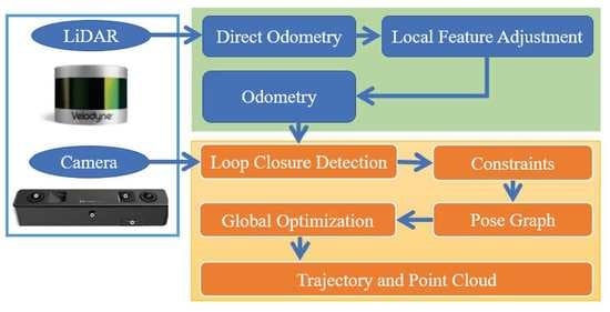
The whole LV-SLAM also includes two parts: front-end odometry and back-end optimization. The system architecture is presented in Figure 1. The front-end used in this paper was an improved LOAM method, and the front-end problem was divided into two modules. One module performed odometry at a high-frequency, but at low fidelity, to estimate the velocity of the laser scanner. A second module ran at a frequency of an order of magnitude lower for fine matching and registration of the point clouds. In the original LOAM, feature points located on sharp edges and planar surfaces are extracted, and the feature points to edge line segments and planar surface patches are matched, respectively. The original LOAM belongs to the feature-based methods. Comparatively, our improved LOAM utilized the normal distributions transform (NDT) method instead of extracting feature points to the scans, matching directly and efficiently in the odometry module. In other words, the NDT-based odometry is referred to as direct odometry (DO). The mapping module is similar to the LOAM algorithm. Therefore, the front-end of the improved LOAM is also called DO-LFA.
The back-end global map optimization (GGO) was to construct global pose map optimization and point clouds map after loop detection. After the front-end DO-LFA outputs the odometry, we first combined the BoW similarity score of the visual image and the point clouds re-matching judgment to realize the loop detection. Then, the edge constraints between the key frames were calculated to construct the pose map of the global key frames. Finally, the graph optimization theory was utilized to reduce the global cumulative error, improve the global trajectory accuracy and map consistency, and obtain the final global motion trajectory and point clouds map.
2.2. Loop Closure Detection
There are two solutions to realize loop closure detection: the geometry-based method and the features-based method. The geometry-based method means detecting the loop closure with the known movement information from the front-end odometer, such as, for example, when the platform returns to a certain position that it passed before, to verify whether there is a loop [28,29]. The geometry-based idea is intuitive and simple, but it is difficult to execute when the accumulated error is large [30]. With regards to the features-based loop closure detection method, it has nothing to do with the state estimation of the front-end and the back-end. It utilizes the similarity detection of two frames of images to detect the loop closure, which eliminates the influence of accumulated errors. The features-based loop closure detection method has been applied to multiple visual SLAM systems [31,32]. However, while using the features similarity in the detection, the current frame needs to be compared and calculated with all previous frames, which requires a large amount of calculation, and it will be invalid for a feature’s repetitive environment, i.e., the decoration of multiple adjacent rooms in a hotel. Due to the explosive development of computer vision and image recognition cognitive technology in recent years, compared to the features’ similarity detection with point clouds, visual images containing various features are more mature and robust in loop closure detection. However, the point clouds can provide more accurate quantitative verification for the loop through re-matching based on the image similarity detection.
Based on the above analysis, we comprehensively considered geometry-based and features-based methods, and made full use of visual and point clouds information. A loop closure detection method utilizing visual features is presented in Figure 2. DO-LFA outputs data (pose, point clouds, and image) after the key frame preprocessing, and preliminary candidate frames were obtained by rough detection based on geometric information, such as the distance of the motion trajectory, and then the suspected loop frames were obtained through the BoWs similarity. Finally, the point clouds re-matching was conducted to verify the suspected loop closure.
The geometric rough detection was based on the pose or odometry output by the DO-LFA, wherein we selected the preliminary candidate frames from the historical key frames and matched with the current frame to carry out loop closure detection. There are three threshold judgment conditions (Figure 3): (1) when the search area threshold d1 (red circle radius) of key frames was less than the threshold range, it might be a potential loop closure frame; (2) the interval threshold d2 must be greater than the threshold; and (3) the ring length threshold d3 should be greater than the threshold. The key frames that meet the above conditions were saved as preliminary candidate loop closure frames for further processing.
2.2.1. Visual BOW Similarity
The bag of words (BoW) model [32,33] originated from the fields of information retrieval and text classification, and is now widely used in the recognition of visual images and loop closure detection in SLAM. The general idea is to use k-means or k-means++ to perform cluster analysis based on image feature points, i.e., SURF or ORB to obtain a “word” vector composed of ID numbers and weights. A K-d tree, with k branch and d depth, is utilized to express the vectors as a dictionary; then the image is described according to the statistical histogram of the word, and finally the similarity is calculated for judgment.
The dictionary training is regarded as an unsupervised classification process. Similar to many models in the field of deep learning, the sample size and scale directly affect the effectiveness of the model. Training a large dictionary may require a machine with large memory and high performance, and it will take a long time. Here, we utilized a large dictionary that is widely used by the open-source community. It is trained from about 2900 images. The size of the dictionary is k = 10 and d = 5, that is, up to 10,000 words. The program uses the open-source library DBOW3 (https://github.com/rmsalinas/DBow3, accessed on 7 June 2021) to assist the implementation.
With the dictionary, the corresponding word wj of the specific features can be retrieved. After obtaining the N features of an image and the corresponding words, it is equivalent to obtaining the histogram of the distribution of the image in the dictionary. However, considering the different importance of different words in distinguishability, they are often weighted, similar to the method in text retrieval, which is called term frequency-inverse document frequency (TF-IDF) [34,35]. TF refers to the frequency of a word in a single image. The higher the frequency of a word in the image, the higher the degree of discrimination.
Assuming an image , the word wi appears mi times, the total amount of the occurrences of all words is , where:
In addition, when the BoW model is established, assuming that the number of all features in the dictionary is n, and the number of features in a leaf node wi is ni, the IDF of the word is defined as:
Then, the weight of wi is the product of TF and IDF
For image A, its multiple feature points retrieve multiple words in the dictionary. Considering the weight, the BoW vector constituting the image is written as:
The number of words in the dictionary is often very large, and there may be only some features and words in the image, and, thus, it will be a sparse vector with a large number of zero values. The non-zero part of describes words corresponding to the features in image A, and the values of non-zero parts are the TF-IDF values.
Therefore, assuming two images A and B, their BoWs vectors and can be obtained. There are multiple representation methods for similarity calculation. Here, we chose the L1 norm to measure their similarity, and the result value falls within the interval (0, 1). If the images are exactly the same, the result is 1, and the similarity calculation is presented as [36]:
In the loop closure detection phase, we calculated the BoW similarity between the current frame and all the candidate frames. The frames with similarity less than 0.05 were directly eliminated, and the rest of the suspected loop closure frames were sorted according to the similarity values, from high to low, and processed in the following step for further verification.
2.2.2. Loop Closure Detection Verifying and Its Accuracy
In order to verify the suspected loop closure frames, we matched the current frame and the suspected loop frames one by one in the sorted order, and counted the Euclidean fitness score for each match. The Euclidean consistency score is the mean value of the square of the distance from the source point clouds to the target point clouds. Corresponding points exceeding a certain threshold are not considered in the calculation. If the score is lower than the threshold (0.2 m), then this frame is the final loop closure frame of the current frame, and the matched relative pose is utilized as a constraint for subsequent pose map optimization.
When detecting the loop closure, there are usually four conditions, which are summarized in the Table 1: true positive (TP), false positive (False Positive, FP), true negative (TN), and false negative (FN). True positives mean that the frame is a loop closure frame; while true negatives mean that the frame is not a loop frame. False positives mean the frame is not a loop closure, but the algorithm judged it to be one; while false negatives mean that the frame is a loop closure, but the algorithm judged it not to be.
In our results, we hoped that TP and TN would appear as much as possible, whereas we hoped that FP and FN would appear as little as possible or not at all. For a certain loop detection algorithm, the frequency of occurrence of TP, TN, FP, and FN on a certain sample data can be counted, and the accuracy (precision) and recall rate (recall) can be calculated:
3. Global Graph Optimization
3.1. Global Pose Construction
Compared with the back-end GGO, the motion trajectory obtained by the DO-LFA is, broadly speaking, referred to as a front-end odometer. It mainly utilizes the point clouds matching between the current frame and adjacent or local multi-frames to estimate the current pose. These point clouds and their features may also be referred to as landmarks. While different from the visual SLAM, the direct method and abovementioned point clouds match method both fix the connection relationship and then solve the Euclidean transformation. In other words, DO-LFA does not optimize the landmarks, and only solves for the pose node.
As time accumulates, the trajectory of the platform will become longer, and the scale of the map will continue to grow. Since the scanning space of LiDAR is always limited, the scale of point clouds or road signs cannot grow indefinitely with the map, and the constraint relationship between the current frame and earlier historical data may no longer exist. In addition, there are errors in direct method matching and feature point method optimization. The cumulative errors obtained by DO-LFA will become larger, and the inconsistency of the global map will become more obvious.
In order to improve the pose accuracy of the key frame nodes and ensure the quality of the global point clouds map, we can save the trajectory of the DO-LFA and construct a back-end global map optimization to reduce the cumulative errors. The global pose graph utilizes the pose of the key frame as the node, and the relative motion between the two pose nodes, obtained by the point clouds matching, is employed as the constraint edge. The nonlinear least squares adjustment method is used to solve the problem to obtain better results.
Figure 4 visually introduces the process of constructing a pose graph, where the arrow is the pose and the blue dashed line is the motion trajectory. Figure 4a presents the DO-LFA, where the red circle may be understood as overlapping point clouds or road signs for matching. The green line represents the constraint between two adjacent frames of DO. The green and red lines together represent the current frame and constraints between historical, local data. In the key frame screening, the pose nodes are reduced, and the trajectory of the DO-LFA is reserved as the constraint edge between the adjacent key frame pose nodes. Figure 4b presents the prepared frames for loop closure detection and global pose graph optimization. Figure 4c presents the loop detection process, where the green arrow represents the current frame being processed, the red dashed line indicates that the loop closure frame is found and constitutes a loop, and the green dashed line is the loop constraint edge after point clouds re-matching. Figure 4d presents the result of the optimization of the global pose graph. The pose nodes and motion trajectories are optimized, the motion trajectory forms a complete loop, and the point clouds consistency is improved.
3.2. Globe Pose Graph Optimization
In the graph optimization theory, the node denotes the pose of the key frame, which is represented by . The edge denotes the relative motion estimation between two pose nodes. The ordinary edge comes from the direct method or point clouds matching in the DO-LFA, and the loop edge comes from the rematch of the point clouds during loop closure detection. The relative motion, , between and nodes can be expressed as:
The corresponding relation of Lie group and Lie algebra is , and it can be written with Lie group:
From the perspective of the construction process of the pose graph, especially after the loop edge is added, the above formula will not be accurately established.
We regarded the edge constraint as the measured value, and the node pose as the estimated value, and, thus, moved the left side of the above formula to the right side, deriving the error equation:
where and are the variables expected to be estimated. We used Lie algebra to find the derivative of these two variables, adding a disturbance to the and , wherein the error equation can be re-written as:
In order to derive the linearization of the Taylor series expansion of the above formula, we introduced the adjoint property of SE (3):
Equation (12) is re-written as:
The Jacobi matrix calculation is written as:
The optimization of the graph is essentially the least squares optimization. Each pose converter is an optimization variable. The perceptual constraint between poses is an edge, and all pose baselines and constraint edges together form a displacement map.
Assuming C denotes the set of all edges in the pose graph, the cost function of the nonlinear least optimization is written as:
where denotes the information matrix used to describe the matching errors of the point clouds. When the number of nodes reaches the set value, the above cost function can be solved by the Gauss-Newton method or LM method, etc. Open-source libraries, i.e., Ceres or g2o, also provide some solution methods for graph optimization.
4. Experiments and Results
4.1. KITTI Dataset
4.1.1. Dataset Description
With the aim of qualitatively evaluating the performance of the proposed method, we employed the open-source KITTI dataset for testing. The KITTI data acquisition platform and the sensors used are shown in Figure 5. The left camera, a Point Grey Flea2 (FL2-14S3C-C), was installed at Cam2. This camera, a classic colorful industrial camera from Point Grey, Canada, has 1.4 million pixels, a global shutter, and an acquisition frequency of 10 HZ. There were a total of seven sequences with loops in the 11 sequences: #00, #05, #06, #07, #02, #08, and #09. We tested all the data from these seven sequences. Some important threshold parameters used in the experiment were set as follows:
(1) The distance and angle thresholds for key frame selection were 10 m and 10°, respectively;
(2) The thresholds d1, d2, and d3, for geometric rough detection, were 20 m, 50 m, and 100 m, respectively.
4.1.2. Results Analysis
In the experiment, all seven sequences with loops were employed in the tests, and all the results with GGO (DO-LFA-GGO) and without GGO (DO-LFA) were saved for analyzing the position accuracy. According to the collection environment, we divided these seven sequences into three categories for analysis and discussion. Sequence #00 and #05 were classified as group A, sequence #06 and #07 were classified as group B, and sequence #02, #09, and #08 were classified as group C; the experimental results are listed in Table 2 and presented in Figure 6, Figure 7 and Figure 8, respectively. The trajectory, loop position, and cumulative position error (CPE) of each group of data are presented.
Group A and group B were both urban environments, including urban roads, many loops, and many regular buildings, and the perceived structure of the environment was better. Group C, on the other hand, was a mixed urban and rural environment with twists and turns in the rural roads. There were few loops and relatively few buildings. Farmland without references existed in this group, and the structure of the perceived environment was poor. The basis for the separation of group A and B was that the DO-LFA accuracy of group A was poor before GGO operation and the accuracy improvement effect was obvious after GGO, whereas the DO-LFA of group B achieved high accuracy and the optimization effect was not obvious.
In the following Figure 6, Figure 7 and Figure 8, the white line denotes the GPS/INS reference trajectory, the green line denotes the trajectory of DO-LFA without GGO, and the blue line denotes the trajectory of DO-LFA with GGO (DO-LFA-GGO). Parts of the trajectories overlap, therefore, it seems that there is only one color for the overlapped trajectories. The red squares mark the detailed position of the loop in the trajectory. Combining with the trajectory and motion details, the counted number of loops was utilized to confirm whether the loop was correct. Moreover, the cumulative position errors with and without GGO are also presented in these figures.
Trajectory, loop closure location, and the CPE values of group A (#00 and #05) are presented in Figure 6. The environment of sequence #00 and #05 was a well-structured town, the time length of the sequence was comparatively long, and the movement distance was long, in excess of 2 km. In total, 15 loop closures were detected in sequence #00, while seven were detected in sequence #05. These loop closures were evenly distributed on the trajectory at an interval of 50 m, which is almost identical to the inter-loop threshold for loop closure detection. The loop closure detection accuracy showed that the accuracy rate reached 100%. The CPE of the DO-LFA of the two sequences were large, reaching 6.71 m and 14.27 m, respectively, and dropped to 0.12 m and 0.36 m, respectively, after GGO. The trajectory of DO-LFA-GGO was also closer than DO-LFA to the true trajectory, which indicated that GGO achieved the expected effect and the CPE was basically eliminated.
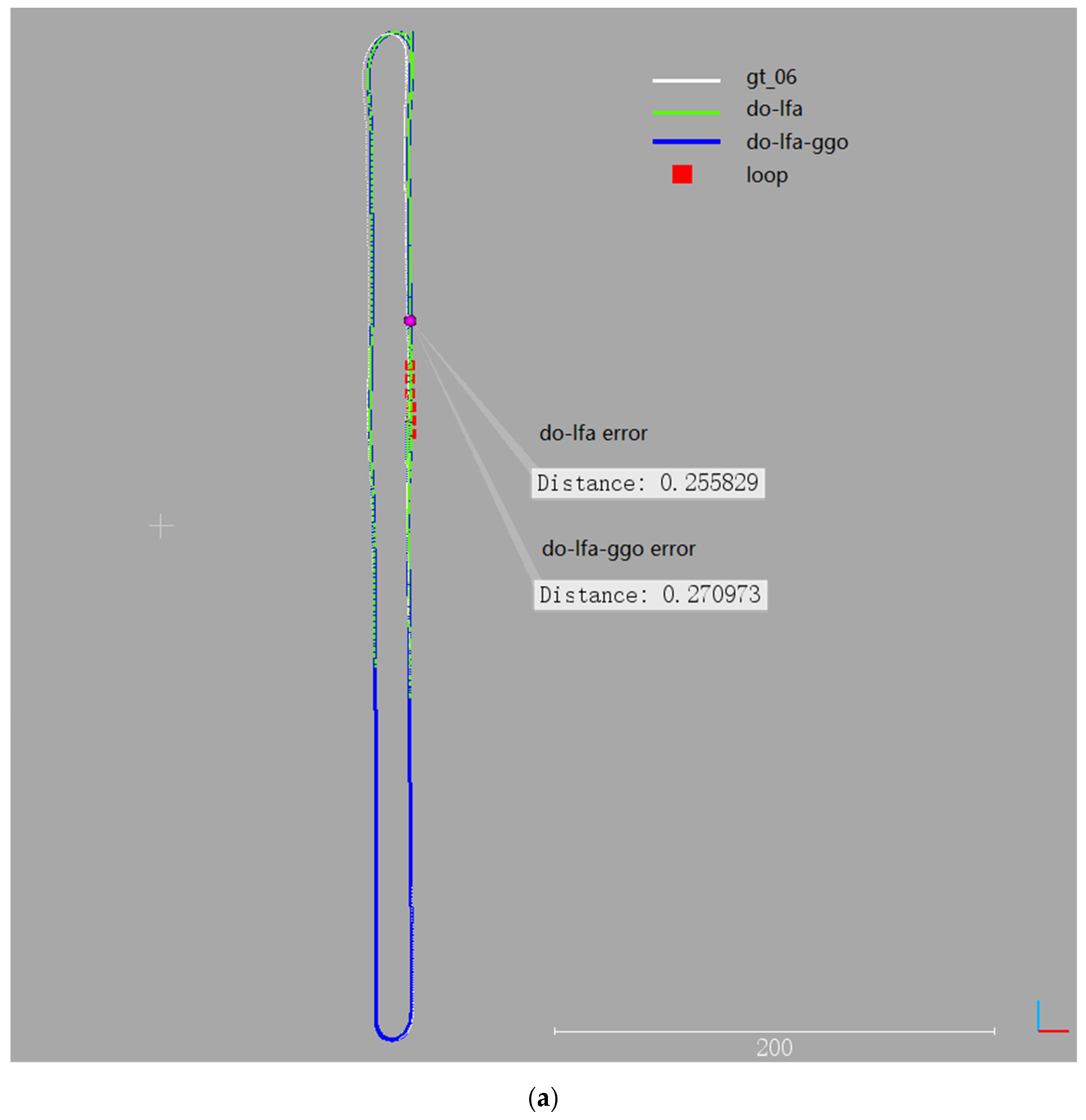
Trajectory, loop closure position, and the CPE of group B data (#06 and #07) are presented in Figure 7. In this trajectory, six loop closures were detected in sequence #06, while sequence #07 had only one loop closure, which was located at the end of the trajectory. The most important finding was that the CPE values of the DO-LFA for these two sequences were small and less than 30 cm and their trajectories almost overlapped with the reference trajectory. After GGO operation, the trajectories and the CPE values did not have any obvious changes, which indicated that the GGO process did not pose any negative influence on the DO-LFA results and that the CPE was still kept small after the GGO operation. The environment of sequence #06 and #07 was a well-structured town, and their scanning time and movement distances were shorter than group A sequences. Therefore, the DO-LFA performed well and the GGO did not effectively reduce the errors.
The environments of group C sequences (#02, #09, and #08) were more complicated. Their trajectories, loop closure positions, and cumulative position error calculations are presented in Figure 8. Many of the paths from the sequences #02, #09, and #08 were in the countryside with winding roads, bends, few loop closures, and relatively few buildings. There was farmland without reference objects on the ground and the structure of the environment were poor.
The collection environment of sequence #02 was a rural road with continuous large turns. There was no loop closure for a long time in the early stage, and only three loop closures were successfully detected during the second half of the trajectory. The CPE values before and after GGO were 8.76 m and 0.13 m, respectively, which showed that the GGO reduced the sequence #02 CPE values. However, we observed that the position errors of the first half were larger than those of the second half due the fact that there was no loop closures detected in the first part of the trajectory.
The environment of sequence #09 also contained a number of consecutive rural roads with large turns. There was also no loop closure in the early stage of the trajectory, and there was only one detected loop closure at the end of the trajectory. The CPE values of the DO-LFA with and without GGO were 4.27 m and 0.09 m, respectively, and the decrease in the CPE indicated that the GGO effectively utilized the detected loop closure and reduced the CPE values. Similar to sequence #02, the trajectory without loop closure performed slightly worse in terms of position errors after the GGO; the long-term continuous country curve and limited looping might account for this phenomenon.
The sequence #08 environment included towns and villages, the roads were regular, there were 2-3 actual loop closure areas, but no loop closure was detected and the recall rate was 0%. The main reason for the loop closure detection failure was that the second time, the travel direction of the vehicle during the loop closure was opposite to that of the first time. Thus, the viewing angle of the sensor scan was also completely opposite, which seriously affected the interpretation of similarity during loop closure detection, especially for image similarity. Without the loop closure, the GGO could not be carried out, and the trajectory with or without GGO was the same.
4.2. WHU Kylin Backpack Experiment
4.2.1. Dataset Description
The major sensors of the WHU Kylin backpack included: Velodyne VLP-16 Lidar, Mynak D1000-IR-120 color binocular camera, Xsens-300 IMU, and a power communication module. An example of the mobile data collection is presented in Figure 9. The average speed of the backpack was 1 m/s, and the data collection and algorithm running speed were both 10 Hz. There were two LiDARs installed on the backpack. In this experiment, only the horizontal LiDAR and the left camera of the binocular camera were used, and the images were 640 × 480 respectively. The backpack was not equipped with a GPS device, so there was no true value of the trajectory. As mentioned, we consciously walk out of a relatively regular matrix area at the beginning and end of the acquisition path for accuracy evaluation. Some important threshold parameters used in the experiment were set as follows: the distance threshold and angle threshold of the key frame selection were 2 m and 10°, respectively; and the thresholds d1, d2, and d3 of the geometric rough detection were 5 m, 15 m, and 25 m, respectively.
With the backpack LiDAR scanning system, we collected three datasets, sequences #01, #02, and #03, to assess the proposed method. The trajectories, loop closure position, and CPE values are presented in the Figure 10, Figure 11 and Figure 12. Similar to the results in the KITTI experiment, the green lines denote the trajectories from the results without DO-LFA, the blue lines denote the trajectories from the DO-LFA-GGA method, and part of the trajectories overlapping led to the corresponding trajectories being presented in one color. The red rectangle denotes the loop closure position in the trajectory, and we counted the loops closure according to the red rectangle and compared it with the motions.
4.2.2. Results and Analysis
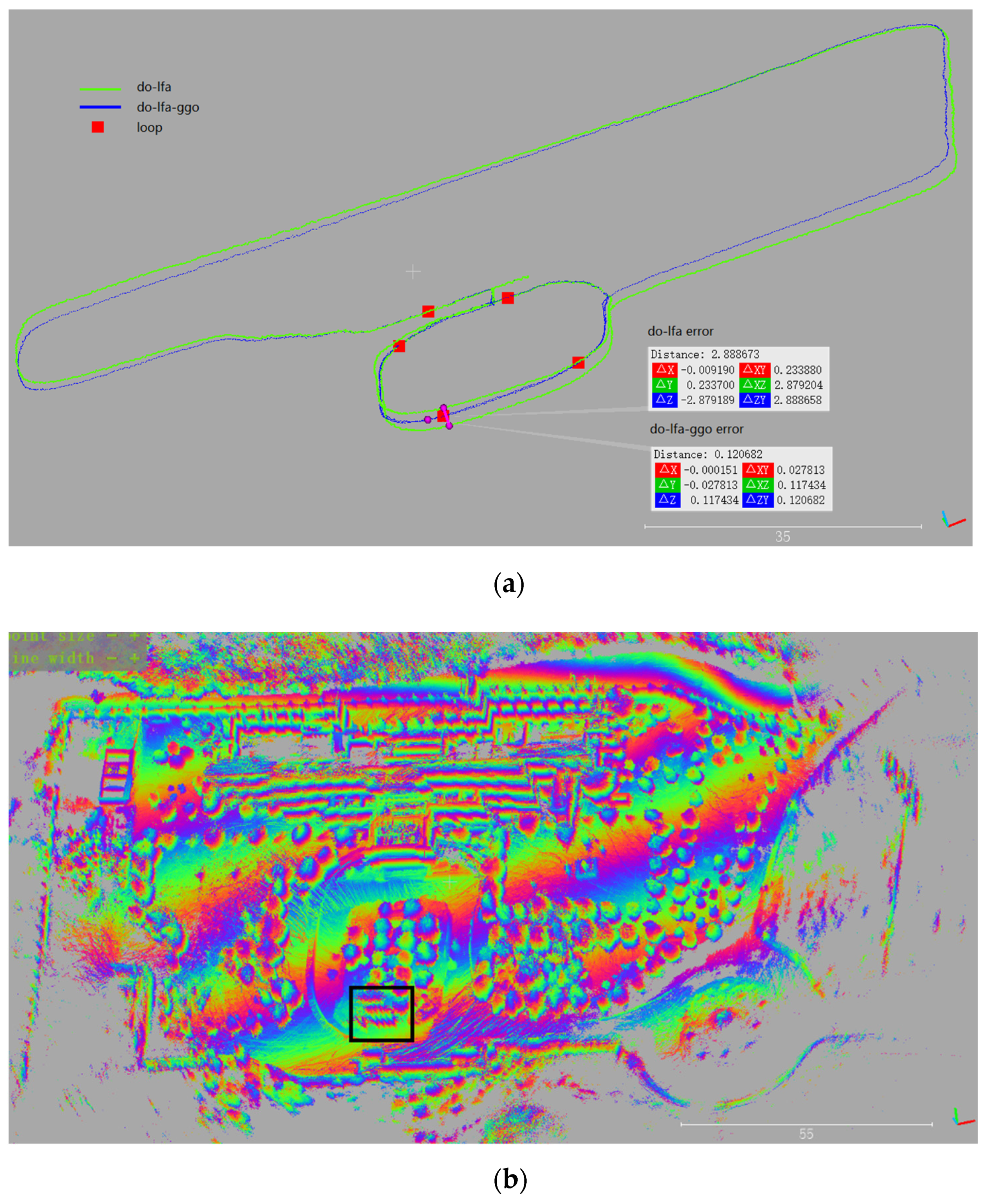
Figure 10 shows the trajectories and point clouds map comparison of sequence #01 with and without GGO. Specifically, Figure 10a presents the trajectory comparison before and after GGO, (b) is the overall point clouds map after GGO, while (c) and (d) are the magnification of the black box area in (b) of the point clouds before and after GGO, respectively.
We observed that the number of loop closures detected in #01 was 5, and that they were evenly distributed on the path with an interval of about 10 m (10 m was also the threshold set for loop closure detection). It showed that the loop closure detection accuracy reached 100%. The CPE of the DO-LFA of sequence #01 was large, reaching 2.89 m. However, it dropped to 0.12 m after GGO processing. The trajectory of DO-LFA-GGO was also more accurate than DO-LFA in the loop, indicating that the GGO achieved the expected effect. The error was basically eliminated to 0.12 m of the DO-LFA-GGO from 2.89 m of the DO-LFA.
Buildings, trees, and flagpoles can be described in detail with the point clouds. Here, through comparing the point clouds map, it can be seen that the trajectory without GGO drifted greatly, the constructed point cloud map had obvious layering and confusion, and its consistency was poor. After using loop closure detection and global map optimization, the optimal estimation of platform poses and point clouds was obtained. Therefore, the consistency of the point clouds map constructed was better, and the layering and disorder of the point clouds at the loop closure location disappeared.
Figure 11 shows the trajectory and point clouds map of sequence #02 with and without GGO. Sequence #02 was an indoor scene of the Huawei Song Research Institute (Xibeipo Village, Songshan Lake, Dongguan) H5. Specifically, Figure 11a presents the comparison of the trajectories from the DO-LFA and DO-LFA-GGO method, while Figure 11b presents the point clouds map from the DO-LFA-GGO, noting that accuracy before GGO was already relatively high and that the point clouds were no longer compared after GGO.
From comparing the trajectories, we observed that the number of loop closures detected in sequence#02 was two, and that the loop closure detection was all correct. The CPE of the DO-LFA method of this sequence was small, and there was little change after performing the GGO. Specifically, the CPE values of the DO-LFA and DO-LFA-GGO were 0.19 m and 0.17 m, respectively. For the trajectory that the DO-LFA worked well for, the DO-LFA-GGO still worked well and kept the CPE values small. In sequence #02, the point clouds map clearly described the trees, buildings, and other objects.
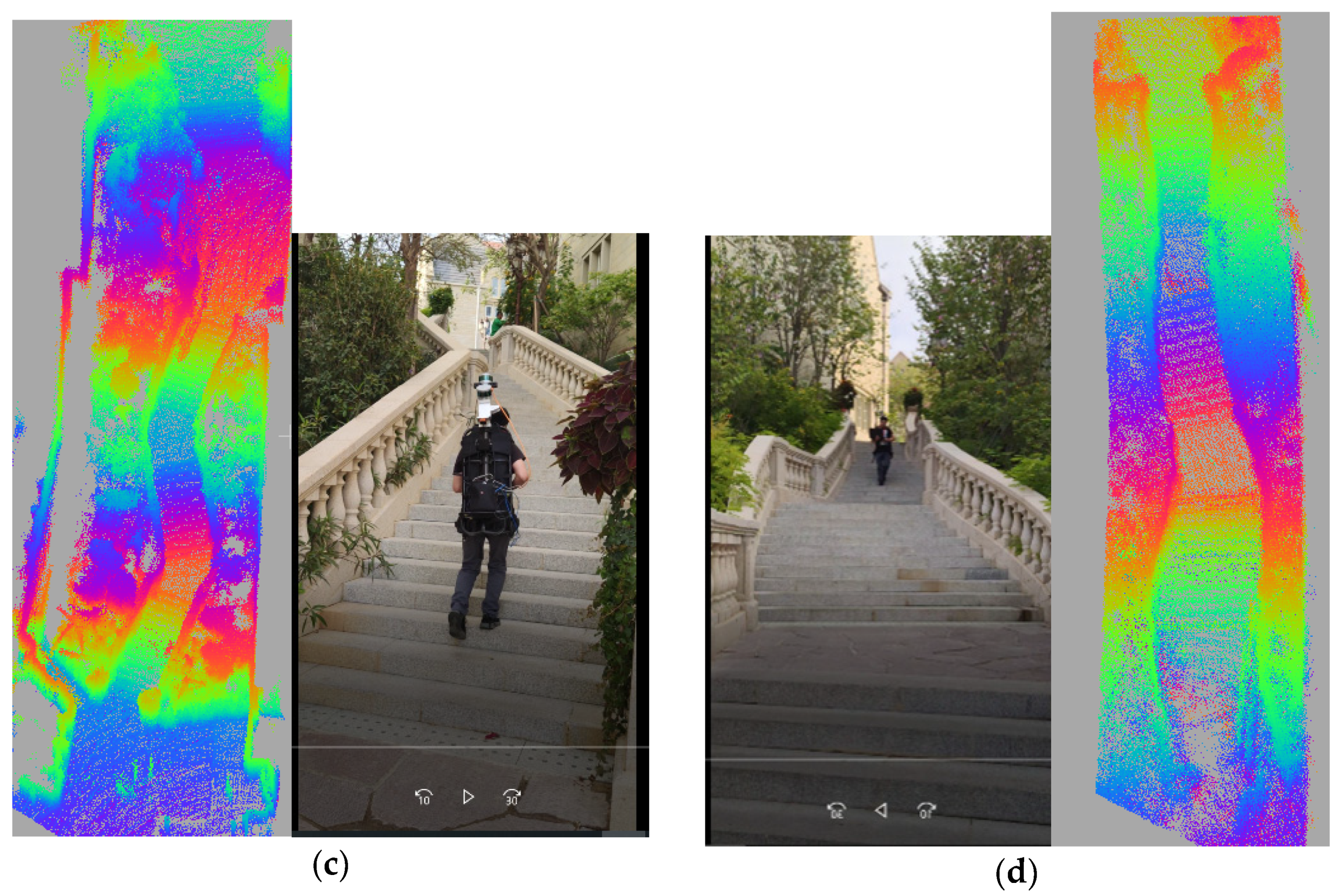
Figure 12 presents the trajectories and point clouds map from the DO-LFA and DO-LFA-GGO methods. Sequence #02 was indoor and outdoor scenes from the Huawei Song Research Institute (Songshan Lake Streamback Slope Village, Dongguan) D4. The terrain was undulating, including up and down stairs. Figure 12a presents the positioning trajectories comparison between the DO-LFA and DO-LFA-GGO, while Figure 12b presents the point clouds map from DO-LFA-GGO. Since the accuracy of the DO-LFA was already relatively high, the point clouds were no longer compared, and Figure 12c and Figure 12d present corresponding point clouds of the slope stairs.
With the plotted trajectories, we observed that six loop closures were detected in sequence #03. The CPE of the DO-LFA in this sequence was small, and there was little change in the CPE while operating the GGO, specifically, the CPE reduced from 0.16 m to 0.15 m. For the high-precision trajectory, the DO-LFA-GGO still maintained its original high precision. The point clouds map had clear and accurate building outlines and targets. The accuracy of the up and down stairs point clouds illustrated the accuracy and robustness of the algorithm to three-dimensional position.
In aspects of the accuracy assessment, although we deliberately collected the data with loop closures, it was difficult to ensure that the front and back positions on the loop revisited path were exactly the same. An error of more than a dozen centimeters (less than the length of a foot) was normal. The CPE values of #00, #01, and #02 after GGO were 0.12 m, 0.17 m, and 0.15 m, respectively, which are all below 20 cm. Considering the original inconsistency of true value motion, the actual error may be lower.
The above three sets of representative datasets included both indoor and outdoor scenes, which suggests that the DO-LFA-GGO proposed in this paper can be successfully operated. When the original DO-LFA had a cumulative position error, GGO significantly eliminated its CPE values. When the original DO-LFA had a higher accuracy, the GGO still maintained its high accuracy. The GGO ensured the accuracy of positioning and the consistency of the point clouds map. The accuracy of global positioning and point clouds mapping can reach less than 20 cm, and it had high robustness via the backpack platform under both indoor and outdoor environments.
4.3. Comparisons with Google Cartographer
The Cartographer developed by Google is a 2D/3D LiDAR SLAM utilizing loop closure detection and graph optimization [33]. We ran the Cartographer with the Kylin #02 and #03 datasets, and the results were compared with that from the DO-LFA-GGO.
Figure 13 and Figure 14 present the point clouds results from the Cartographer with the Kylin #02 and #03 datasets. The color of the point clouds from the Cartographer were determined by the LiDAR backscatter laser intensity. Confusion and ghosts are all the result of coaxial progressive errors, and the displacement error roughly measured by the point clouds was approximately 5–10 m. The DLO-LFA-GGO in this paper detected the loop closure based on visual BoW similarity and conducted the point clouds re-matching to achieve fusion of the two data. However, the Cartographer detects the loop closure with the point clouds similarity. As a result, the point clouds from the Cartographer have severe layering and ghosting at the loop repeats, with a displacement error up to 5–10 m; while the point clouds maps from the DO-LFA-GGO have clear and accurate targets with high consistency, and the geometric CPE is only approximately 20 cm.
5. Conclusions
In this paper, we investigated a LiDAR SLAM back-end graph optimization methods using visual features to improve loop closure detection and graph optimization performance. With both experiments in open-source KITTI datasets and a self-developed back-pack lasering scanning system, we can conclude that:
(1) Visual features can efficiently improve loop closure detection accuracy;
(2) With the detection loop closure, the graph optimization reduced the CPE values of the LiDAR SLAM through the point clouds re-matching;
(3) Compared with Cartographer, LiDAR based SLAM, our LiDAR/visual SLAM with loop closure detection and global graph optimization achieved much better performance, including better point clouds map and CPE values.
The source code of this paper was uploaded to the GitHub website and is open source for readers. We expect that the work in this paper will inspire some other interesting investigations into visual/LiDAR SLAM. Although a satisfying performance was obtained, the following work is of great significance for further investigation.
(1) In this paper, to guarantee the accuracy of loop closure detection using visual features, we set strict parameters and rules, which led to some loop closures being missed. Thus a more robust loop closure detection strategy is of great significance for improving the use of visual/LiDAR SLAM in complex environments;
(2) As presented in the experiment, different trajectories had different numbers and positions of detected loop closures. It is therefore interesting to explore the influence of the loop closure number and distributions on the GGO performance.
(3) In this paper, we utilized the visual features in back-end graph optimization, and so, it would be interesting to explore visual/LiDAR based front-end odometry.
(4) Visual/LiDAR are the most popular sensors in environmental perception. Based on the code used in this paper, it is prospective to integrate other sensors, i.e., GNSS and IMU, to the current visual/LiDAR SLAM in the graph optimization framework.
Author Contributions
Methodology, S.C.; software, S.C.; writing—original draft preparation, C.S. and C.J.; writing—review and editing, C.J.; supervision, Q.L.; system development, B.Z. and W.X.; dataset collection and experiments conducting. All authors have read and agreed to the published version of the manuscript.
Funding
This study was supported in part by the National Key R&D Program of China (2016YFB0502203), Guangdong Basic and Applied Basic Research Foundation (2019A1515011910), Shenzhen Science and Technology program (KQTD20180412181337494, JCYJ20190808113603556) and the State Scholarship Fund of China Scholarship Council (201806270197).
Data Availability Statement
The source code of the paper is uploaded to GitHub and its link is https://github.com/BurryChen/lv_slam (accessed on 7 June 2021).
Acknowledgments
Thank you to State Key Laboratory of Information Engineering in Surveying, Mapping and Remote Sensing in Wuhan University for technical support and data collection support. Thank you to the anonymous reviewers who provided detailed feedback that guided the improvement of this manuscript during the review process.
Conflicts of Interest
The authors declare no conflict of interest.
References
- Bailey, T.; Durrant-Whyte, H. Simultaneous localization and mapping (SLAM): Part II. IEEE Robot. Autom. Mag. 2006, 13, 108–117. [Google Scholar] [CrossRef] [Green Version]
- Cadena, C.; Carlone, L.; Carrillo, H.; Latif, Y.; Scaramuzza, D.; Neira, J.; Reid, I.; Leonard, J.J. Past, present, and future of simultaneous localization and mapping: Toward the robust-perception age. IEEE Trans. Robot. 2016, 32, 1309–1332. [Google Scholar] [CrossRef] [Green Version]
- Zhou, B.; Ma, W.; Li, Q.; El-Sheimy, N.; Mao, Q.; Li, Y.; Zhu, J. Crowdsourcing-based indoor mapping using smartphones: A survey. ISPRS J. Photogramm. Remote Sens. 2021, 177, 131–146. [Google Scholar] [CrossRef]
- Gao, X.; Wang, R.; Demmel, N.; Cremers, D. LDSO: Direct sparse odometry with loop closure. In Proceedings of the 2018 IEEE/RSJ International Conference on Intelligent Robots and Systems (IROS), Madrid, Spain, 1–5 October 2018; pp. 2198–2204. [Google Scholar]
- Engel, J.; Koltun, V.; Cremers, D. Direct sparse odometry. IEEE Trans. Pattern Anal. Mach. Intell. 2017, 40, 611–625. [Google Scholar] [CrossRef] [PubMed]
- Klein, G.; Murray, D. Parallel tracking and mapping for small AR workspaces. In Proceedings of the 2007 6th IEEE and ACM International Symposium on Mixed and Augmented Reality, Nara, Japan, 13–16 November 2007; pp. 225–234. [Google Scholar]
- Mur-Artal, R.; Tardos, J.D. ORB-SLAM2: An open-source SLAM system for monocular, stereo, and RGB-D cameras. IEEE Trans. Robot. 2017, 33, 1255–1262. [Google Scholar] [CrossRef] [Green Version]
- Hess, W.; Kohler, D.; Rapp, H.; Andor, D. Real-time loop closure in 2D LIDAR SLAM. In Proceedings of the 2016 IEEE International Conference on Robotics and Automation (ICRAE), Jeju-Do, Korea, 27–29 August 2016; pp. 1271–1278. [Google Scholar]
- Zhang, J.; Singh, S. Low-drift and real-time lidar odometry and mapping. Auton. Robot. 2017, 41, 401–416. [Google Scholar] [CrossRef]
- Grisetti, G.; Stachniss, C.; Burgard, W. Improved techniques for grid mapping with rao-blackwellized particle filters. IEEE Trans. Robot. 2007, 23, 34. [Google Scholar] [CrossRef] [Green Version]
- Sturm, J.; Engelhard, N.; Endres, F.; Burgard, W.; Cremers, D. A benchmark for the evaluation of RGB-D SLAM systems. In Proceedings of the 2012 IEEE/RSJ International Conference on Intelligent Robots and Systems, Vilamoura-Algarve, Portugal, 7–12 October 2012; pp. 573–580. [Google Scholar]
- Qin, T.; Li, P.; Shen, S. VINS-mono: A robust and versatile monocular visual-inertial state estimator. IEEE Trans. Robot. 2018, 34, 1004–1020. [Google Scholar] [CrossRef] [Green Version]
- Shen, S.; Michael, N.; Kumar, V. Autonomous multi-floor indoor navigation with a computationally constrained MAV. In Proceedings of the 2011 IEEE International Conference on Robotics and Automation, Shanghai, China, 9–13 May 2011; pp. 20–25. [Google Scholar]
- Shen, S.; Michael, N.; Kumar, V. Tightly coupled monocular visual-inertial fusion for autonomous flight of rotorcraft MAVs. In Proceedings of the 2015 IEEE International Conference on Robotics and Automation (ICRA), Seattle, WA, USA, 26–30 May 2015; pp. 5303–5310. [Google Scholar] [CrossRef]
- Engel, J.; Schöps, T.; Cremers, D. LSD-SLAM: Large-scale direct monocular SLAM. In Proceedings of the 13th European Conference of Computer Vision, Zürich, Switzerland, 6–12 September 2014; pp. 834–849. [Google Scholar]
- Forster, C.; Pizzoli, M.; Scaramuzza, D. SVO: Fast semi-direct monocular visual odometry. In Proceedings of the IEEE International Conference on Robotics and Automation (ICRA), Hong Kong, China, 31 May–7 June 2014; pp. 15–22. [Google Scholar]
- Wang, R.; Schworer, M.; Cremers, D. Stereo DSO: Large-scale direct sparse visual odometry with stereo cameras. In Proceedings of the 2017 IEEE International Conference on Computer Vision (ICCV), Venice, Italy, 22–29 October 2017; pp. 3923–3931. [Google Scholar]
- Thrun, S. Probabilistic robotics. Commun. ACM 2002, 45, 52–57. [Google Scholar] [CrossRef]
- Vincent, R.; Limketkai, B.; Eriksen, M. Comparison of indoor robot localization techniques in the absence of GPS. In Detection and Sensing of Mines, Explosive Objects, and Obscured Targets XV; Harmon, R.S., Holloway, J.H., Jr., Broach, J.T., Eds.; International Society for Optics and Photonics: Bellingham, WA, USA, 2010; Volume 76641. [Google Scholar]
- Thrun, S.; Montemerlo, M. The graph SLAM algorithm with applications to large-scale mapping of urban structures. Int. J. Robot. Res. 2006, 25, 403–429. [Google Scholar] [CrossRef]
- Olson, E.B. Real-time correlative scan matching. In Proceedings of the 2009 IEEE International Conference on Robotics and Automation, Kobe, Japan, 12–17 May 2009; pp. 4387–4393. [Google Scholar] [CrossRef] [Green Version]
- Zhang, J.; Kaess, M.; Singh, S. A real-time method for depth enhanced visual odometry. Auton. Robot. 2017, 41, 31–43. [Google Scholar] [CrossRef]
- Graeter, J.; Wilczynski, A.; Lauer, M. LIMO: LiDAR-monocular visual odometry. In Proceedings of the 2018 IEEE/RSJ International Conference on Intelligent Robots and Systems (IROS), Madrid, Spain, 1–5 October 2018; pp. 7872–7879. [Google Scholar]
- Shin, Y.S.; Park, Y.S.; Kim, A. Direct visual slam using sparse depth for camera-LiDAR system. In Proceedings of the IEEE International Conference on Robotics and Automation (ICRA), Brisbane, Australia, 21–25 May 2018; pp. 5144–5151. [Google Scholar]
- Shao, W.; Vijayarangan, S.; Li, C.; Kantor, G. Stereo visual inertial LiDAR simultaneous localization and mapping. In Proceedings of the 2019 IEEE/RSJ International Conference on Intelligent Robots and Systems (IROS), Macau, China, 3–8 November 2019; pp. 370–377. [Google Scholar]
- Zhang, J.; Singh, S. Laser-visual-inertial odometry and mapping with high robustness and low drift. J. Field Robot. 2018, 35, 1242–1264. [Google Scholar] [CrossRef]
- Zhang, J.; Singh, S. Visual-lidar odometry and mapping: Low-drift, robust, and fast. Proceedings of 2015 IEEE International Conference on Robotics and Automation (ICRA), Seattle, WA, USA, 26–30 May 2015; pp. 2174–2181. [Google Scholar]
- Hahnel, D.; Burgard, W.; Fox, D.; Thrun, S. An efficient FastSLAM algorithm for generating maps of large-scale cyclic environments from raw laser range measurements. In Proceedings of the 2003 IEEE/RSJ International Conference on Intelligent Robots and Systems (IROS), Las Vegas, NV, USA, 27–31 October 2003; Volume 1, pp. 206–211. [Google Scholar]
- Beeson, P.; Modayil, J.; Kuipers, B. Factoring the mapping problem: Mobile robot map-building in the hybrid spatial semantic hierarchy. Int. J. Robot. Res. 2009, 29, 428–459. [Google Scholar] [CrossRef]
- Latif, Y.; Cadena, C.; Neira, J. Robust loop closing over time for pose graph SLAM. Int. J. Robot. Res. 2013, 32, 1611–1626. [Google Scholar] [CrossRef]
- Ulrich, I.; Nourbakhsh, I. Appearance-based place recognition for topological localization. In Proceedings of the 2000 ICRA. Millennium Conference. IEEE International Conference on Robotics and Automation, San Francisco, CA, USA, 24–28 April 2000; Volume 2, pp. 1023–1029. [Google Scholar] [CrossRef] [Green Version]
- Galvez-Lopez, D.; Tardos, J.D. Real-time loop detection with bags of binary words. In Proceedings of the 2011 IEEE/RSJ International Conference on Intelligent Robots and Systems, San Francisco, CA, USA, 25–30 September 2011; pp. 51–58. [Google Scholar]
- Galvez-Lopez, D.; Tardos, J.D. Bags of binary words for fast place recognition in image sequences. IEEE Trans. Robot. 2012, 28, 1188–1197. [Google Scholar] [CrossRef]
- Sivic, J.; Zisserman, A. Video Google: A text retrieval approach to object matching in videos. In Proceedings of the IEEE International Conference on Computer Vision (ICCV), Nice, France, 13–16 October 2003; p. 1470. [Google Scholar]
- Robertson, S. Understanding inverse document frequency: On theoretical arguments for IDF. J. Doc. 2004, 503–520. [Google Scholar] [CrossRef] [Green Version]
- Nister, D.; Stewenius, H. Scalable recognition with a vocabulary tree. In Proceedings of the IEEE Computer Society Conference on Computer Vision and Pattern Recognition (CVPR), New York, NY, USA, 17–22 June 2006; pp. 2161–2168. [Google Scholar]
Figure 1.
System architecture.

Figure 2.
Flow-chart of the loop closure detection.

Figure 3.
Thresholds for geometry rough detection.

Figure 4.
Pose graph construction: (a) DO-LFA nodes and landmarks; (b) key frames pose node and constraint edges; (c) progress of the pose closure detection; and (d) global pose optimization results.
Figure 4.
Pose graph construction: (a) DO-LFA nodes and landmarks; (b) key frames pose node and constraint edges; (c) progress of the pose closure detection; and (d) global pose optimization results.

Figure 5.
KITTI data collecting platform: (a) position relationship of the installed sensors; (b) Velodyne HDL-64 LiDAR; and the (c) Point Grey Flea 2 (FL2-14S3C-C) colorful camera, installed in the Cam2 position in (a).
Figure 5.
KITTI data collecting platform: (a) position relationship of the installed sensors; (b) Velodyne HDL-64 LiDAR; and the (c) Point Grey Flea 2 (FL2-14S3C-C) colorful camera, installed in the Cam2 position in (a).

Figure 6.
Experimental results from group A: (a) trajectory, loop closure, and position errors for sequence #00; and (b) trajectory, loop closure, and position errors for sequence #05.
Figure 6.
Experimental results from group A: (a) trajectory, loop closure, and position errors for sequence #00; and (b) trajectory, loop closure, and position errors for sequence #05.

Figure 7.
Experimental results from the group B: (a) trajectory, loop closure, and position errors for sequence #06; and (b) trajectory, loop closure, and position errors for sequence #07.
Figure 7.
Experimental results from the group B: (a) trajectory, loop closure, and position errors for sequence #06; and (b) trajectory, loop closure, and position errors for sequence #07.


Figure 8.
Experimental results from group C: (a) trajectory, loop closure, and position errors for sequence #02; (b) trajectory, loop closure, and position errors for sequence #09; and (c) trajectory, loop closure, and position errors for sequence #08.
Figure 8.
Experimental results from group C: (a) trajectory, loop closure, and position errors for sequence #02; (b) trajectory, loop closure, and position errors for sequence #09; and (c) trajectory, loop closure, and position errors for sequence #08.


Figure 9.
WHU Kylin backpack laser scanning platform: (a) data collecting and sensors installation; (b) Velodyne VLP-16 LiDAR; and (c) MYNT D1000-IR-120 color binocular camera.
Figure 9.
WHU Kylin backpack laser scanning platform: (a) data collecting and sensors installation; (b) Velodyne VLP-16 LiDAR; and (c) MYNT D1000-IR-120 color binocular camera.

Figure 10.
Kylin #01 experimental results in Wuhan University: (a) comparisons between trajectories with and without GGO; (b) point clouds map after GGO; while (c,d) present the zoom out point clouds map marked with a black rectangle in (b).
Figure 10.
Kylin #01 experimental results in Wuhan University: (a) comparisons between trajectories with and without GGO; (b) point clouds map after GGO; while (c,d) present the zoom out point clouds map marked with a black rectangle in (b).


Figure 11.
Kylin #02 experimental results in Huawei Songshan Lake Research Institute H5 building: (a) comparisons between trajectories with and without GGO; and (b) point clouds map after GGO.
Figure 11.
Kylin #02 experimental results in Huawei Songshan Lake Research Institute H5 building: (a) comparisons between trajectories with and without GGO; and (b) point clouds map after GGO.

Figure 12.
Kylin #03 experimental results in Huawei Songshan Lake Research Institute D4 building: (a) comparisons between trajectories with and without GGO; (b) point clouds map after GGO; and (c,d) present the data collecting environments and the point clouds.
Figure 12.
Kylin #03 experimental results in Huawei Songshan Lake Research Institute D4 building: (a) comparisons between trajectories with and without GGO; (b) point clouds map after GGO; and (c,d) present the data collecting environments and the point clouds.


Figure 13.
Kylin #02 Cartographer point clouds map: (a) global point clouds map; and (b) zoom out of the point clouds map of the loop closure part.
Figure 13.
Kylin #02 Cartographer point clouds map: (a) global point clouds map; and (b) zoom out of the point clouds map of the loop closure part.

Figure 14.
Kylin #03 Cartographer: (a) global point clouds map; and (b) zoom out of the point clouds map of the loop closure part.
Figure 14.
Kylin #03 Cartographer: (a) global point clouds map; and (b) zoom out of the point clouds map of the loop closure part.


Table 1.
Loop closure detection examples.
| Detection Results Reference | True | False |
|---|---|---|
| True | True Positive | False Positive |
| False | False Negative | True Negative |
Table 2.
KITTI data loop closure detection and global graph optimization (GGO) results.
| Group | Sequences | Environment | Distance (m) | Amount of Detected Loop Closure | Accuracy (%) | Errors before GGO (m) | Errors after GGO (m) |
|---|---|---|---|---|---|---|---|
| A | #00 | Urban | 3723 | 15 | 100% | 6.71 | 0.12 |
| #05 | 2205 | 7 | 100% | 14.27 | 0.36 | ||
| B | #06 | Urban | 1232 | 6 | 100% | 0.26 | 0.27 |
| #07 | 694 | 1 | 100% | 0.29 | 0.21 | ||
| C | #02 | Urban + Rural | 5067 | 3 | 100% | 8.76 | 0.13 |
| #09 | 1705 | 1 | 100% | 0.23 | 0.09 | ||
| #08 | 3222 | 0 | - | - | - |
Publisher’s Note: MDPI stays neutral with regard to jurisdictional claims in published maps and institutional affiliations. |
© 2021 by the authors. Licensee MDPI, Basel, Switzerland. This article is an open access article distributed under the terms and conditions of the Creative Commons Attribution (CC BY) license (https://creativecommons.org/licenses/by/4.0/).
Share and Cite
MDPI and ACS Style
Chen, S.; Zhou, B.; Jiang, C.; Xue, W.; Li, Q. A LiDAR/Visual SLAM Backend with Loop Closure Detection and Graph Optimization. Remote Sens. 2021, 13, 2720. https://0-doi-org.brum.beds.ac.uk/10.3390/rs13142720
AMA Style
Chen S, Zhou B, Jiang C, Xue W, Li Q. A LiDAR/Visual SLAM Backend with Loop Closure Detection and Graph Optimization. Remote Sensing. 2021; 13(14):2720. https://0-doi-org.brum.beds.ac.uk/10.3390/rs13142720
Chicago/Turabian StyleChen, Shoubin, Baoding Zhou, Changhui Jiang, Weixing Xue, and Qingquan Li. 2021. "A LiDAR/Visual SLAM Backend with Loop Closure Detection and Graph Optimization" Remote Sensing 13, no. 14: 2720. https://0-doi-org.brum.beds.ac.uk/10.3390/rs13142720
Note that from the first issue of 2016, this journal uses article numbers instead of page numbers. See further details here.