
Mapping Tree Height in Burkina Faso Parklands with TanDEM-X

 , , , ,
Abstract
:1. Introduction
2. Method
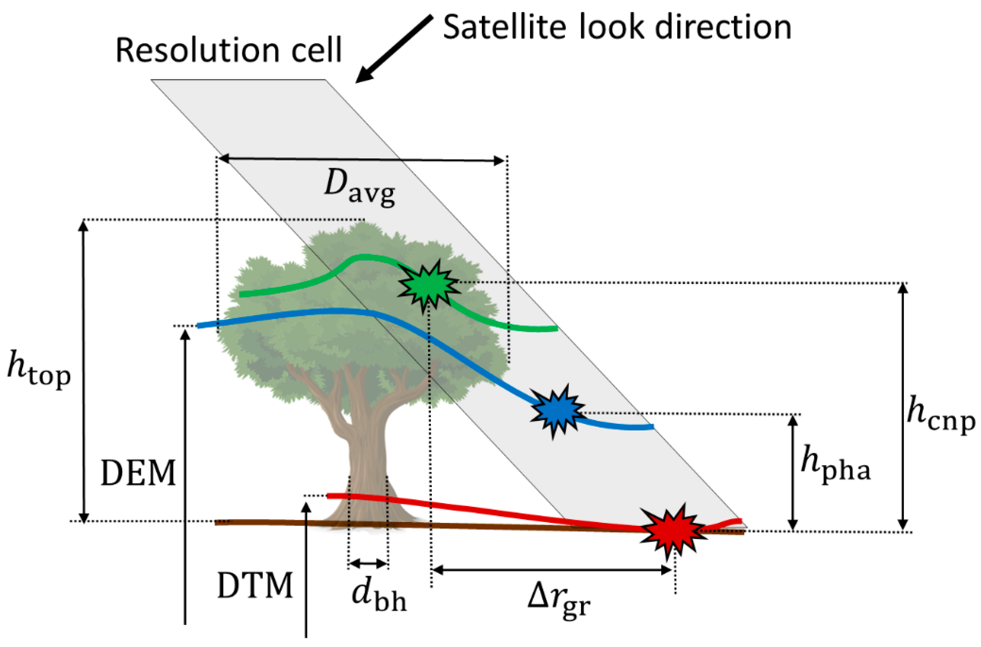
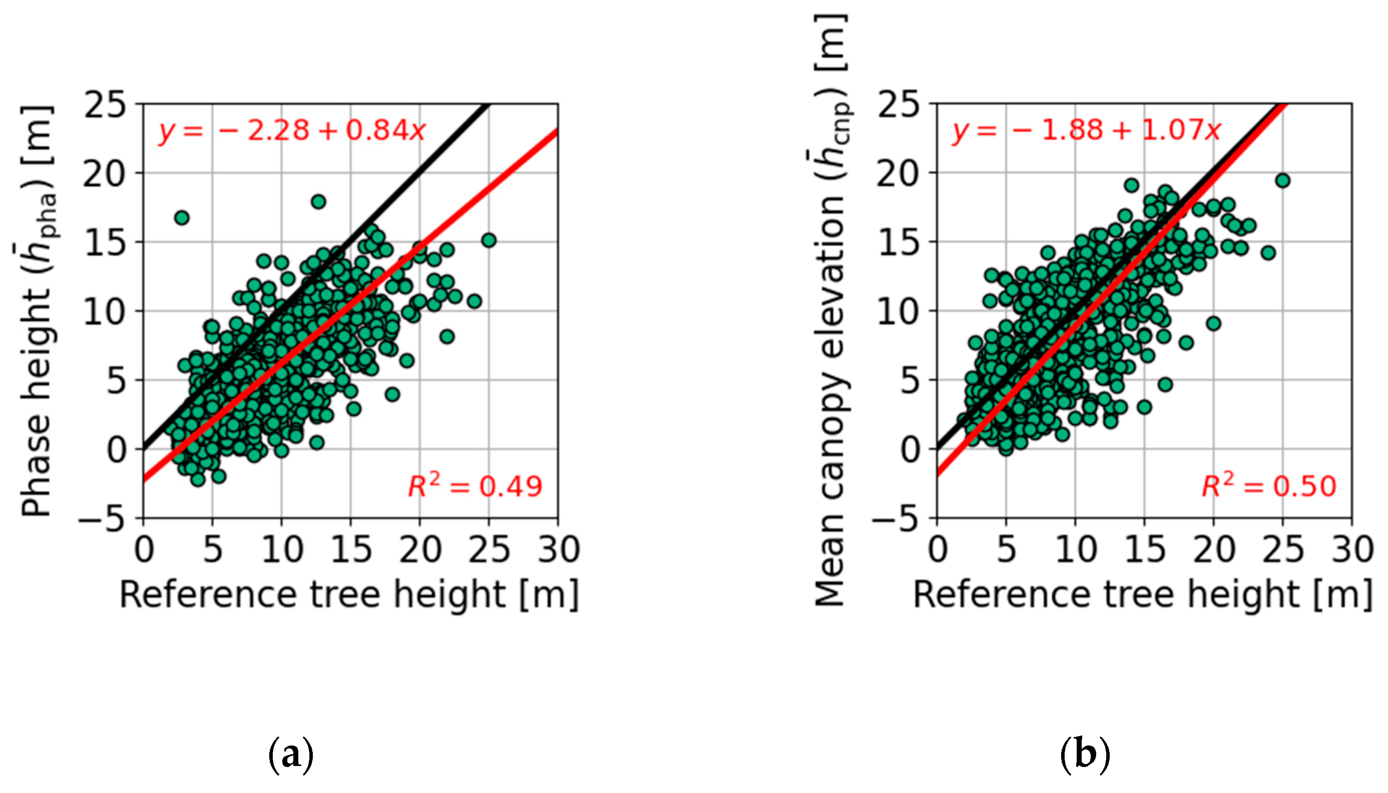
2.1. Phase Height
2.2. Mean Canopy Elevation
2.3. Estimation of Tree Height
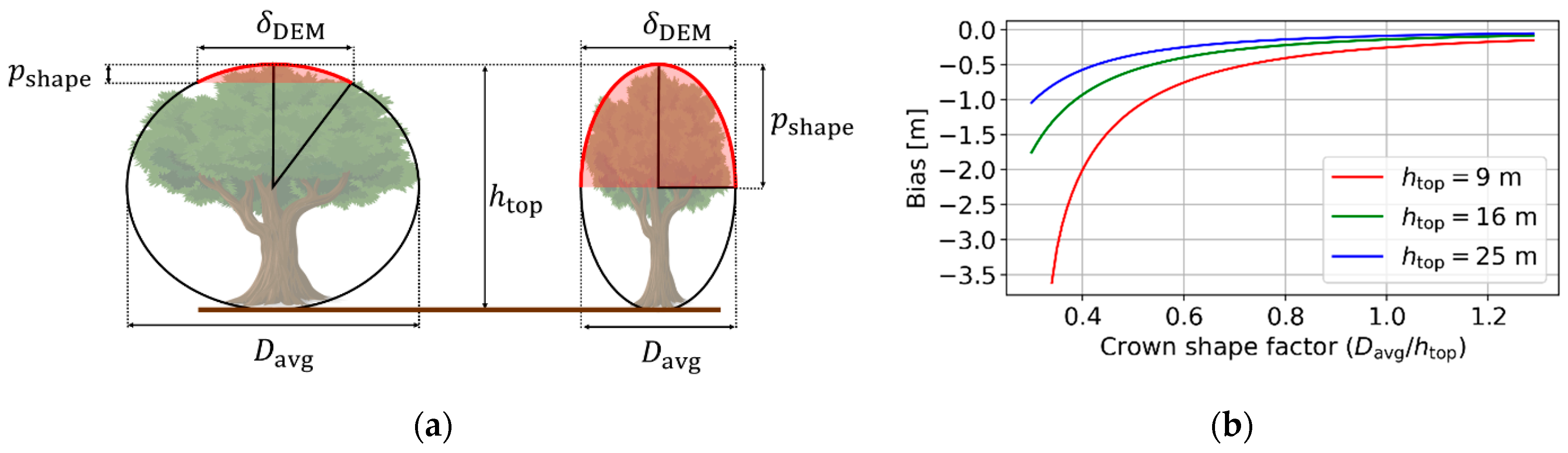
2.3.1. Effect of Crown Shape
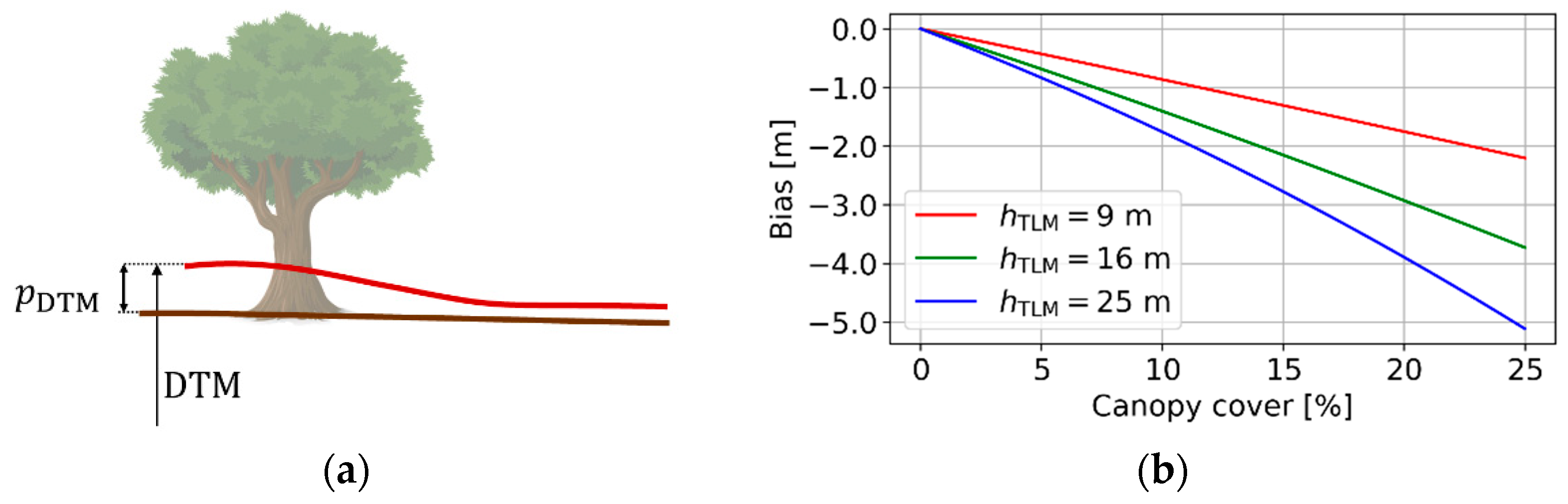
2.3.2. Effect of Vegetation Bias from the DTM
3. Experimental Data
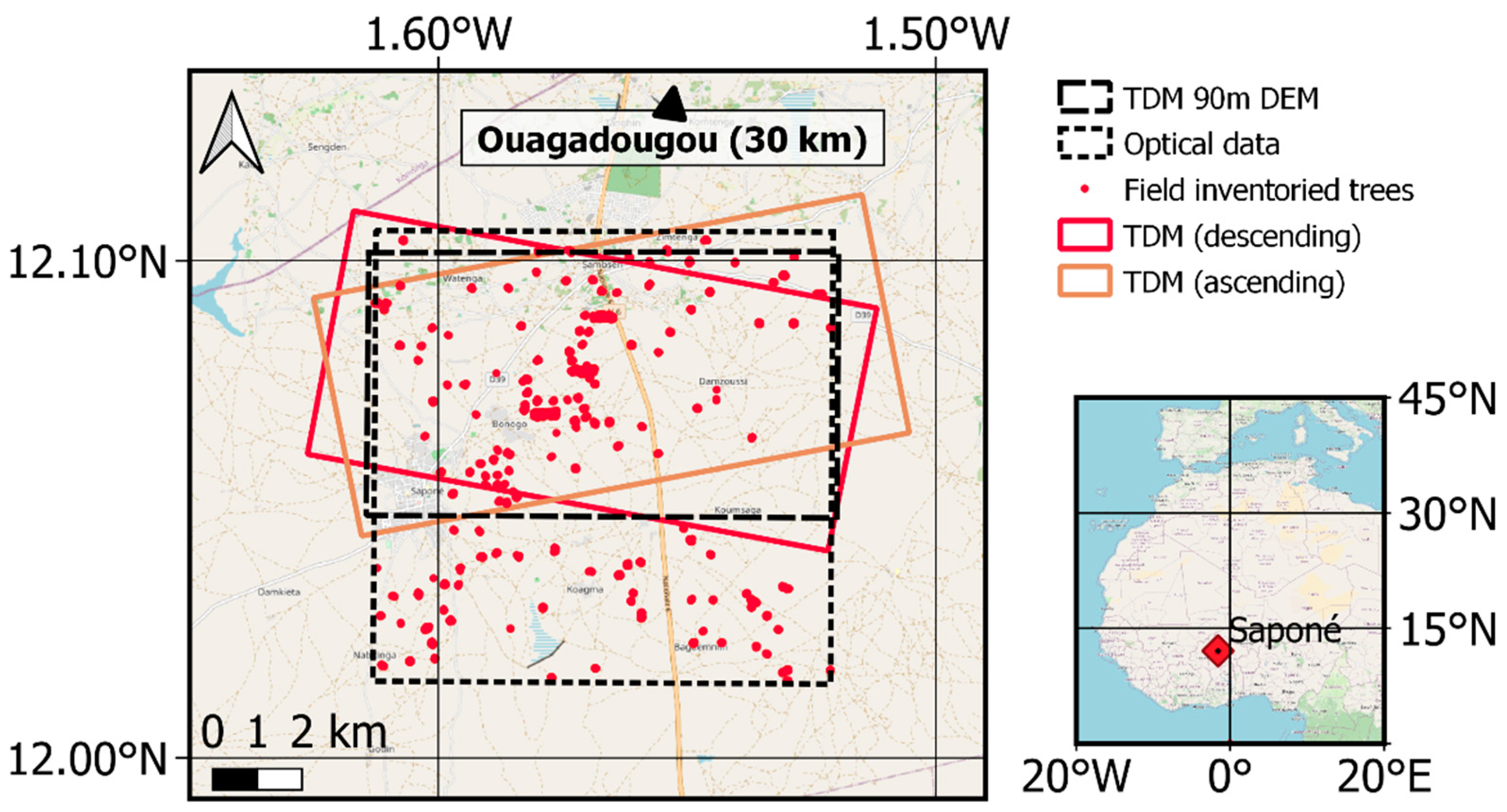
3.1. Test Site
3.2. Reference Data
3.3. TanDEM-X Data Processing
3.4. Estimation of Tree Height from Phase Height and Mean Canopy Elevation
- (i)
- Linear:
- (ii)
- Logarithmic:
- (i)
- Calibrated phase height:
- (ii)
- Calibrated mean canopy elevation:where and are calibration constants estimated from the data. We investigated all possible variants of (10) with between one and seven parameters (i.e., up to six of the seven parameters set to zero), excluding the trivial case of a constant model (). For each of the models, model parameters were estimated twice: once jointly for all tree species/genera, and once individually for each species/genus. This resulted in a total of 760 models. Depending on the type of data used, these 760 models consisted of 16 models using TDM data only, 248 with in situ data only, and 496 models that combined in situ and TDM data.
4. Results
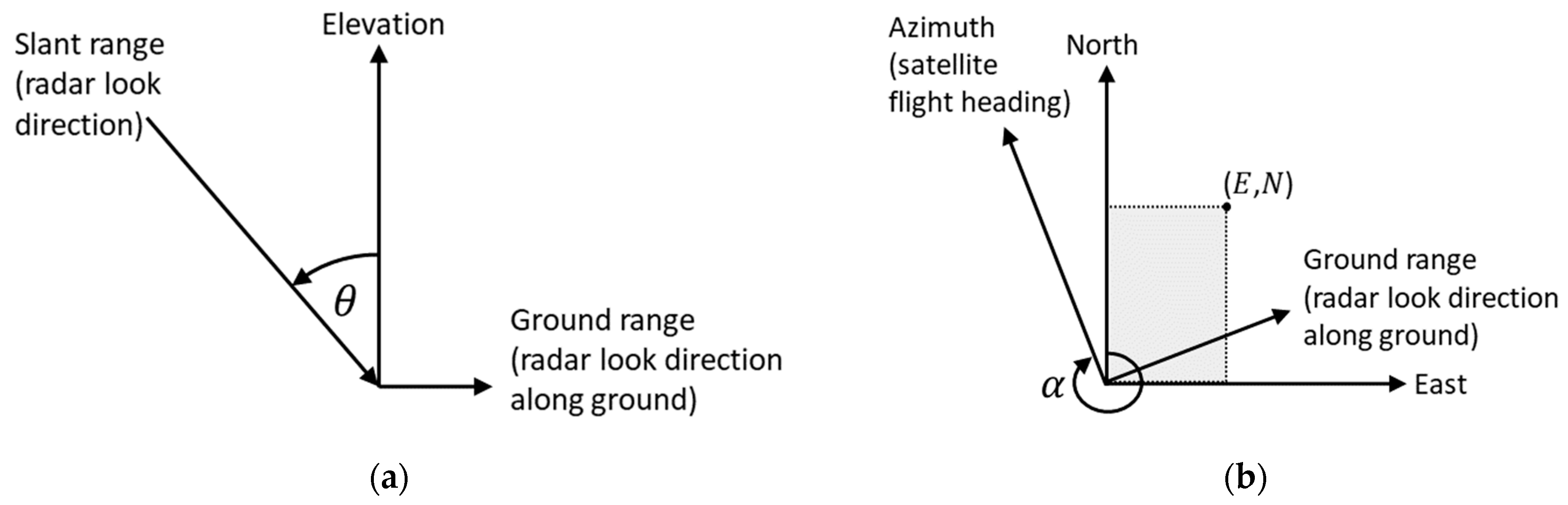
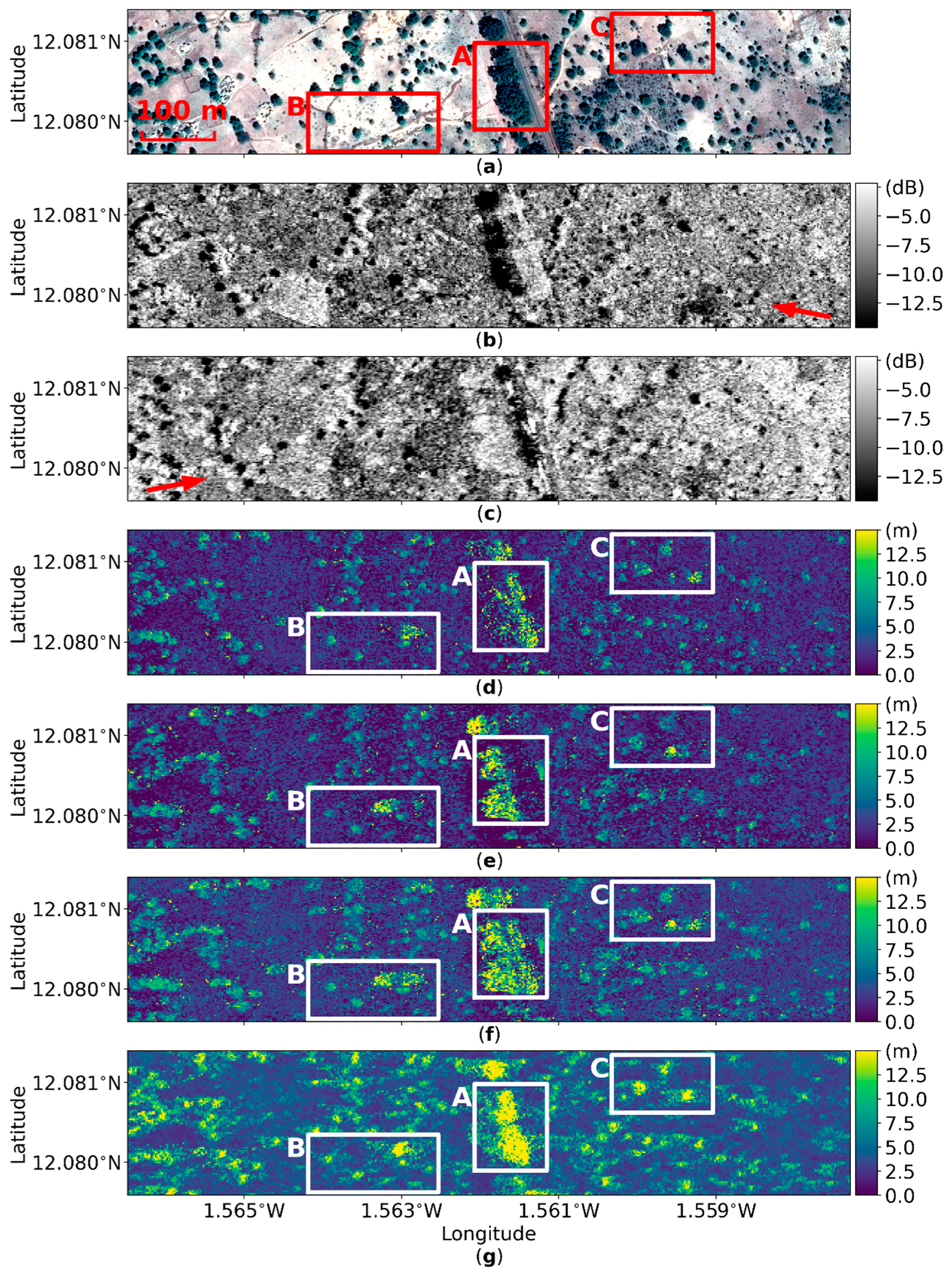
4.1. Geometric Distortion
4.2. Tree Positioning Accuracy
4.3. Tree Height Estimation
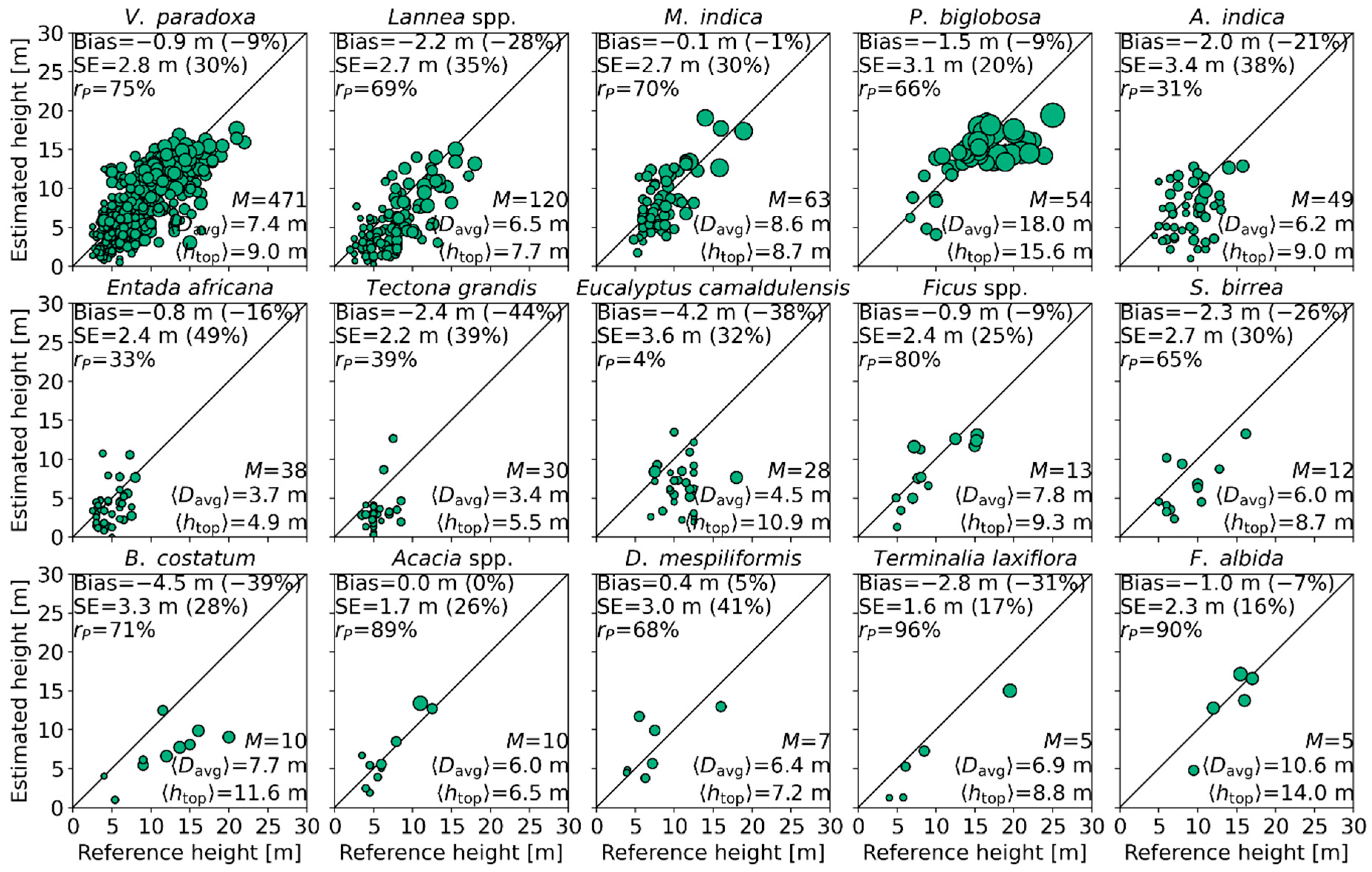
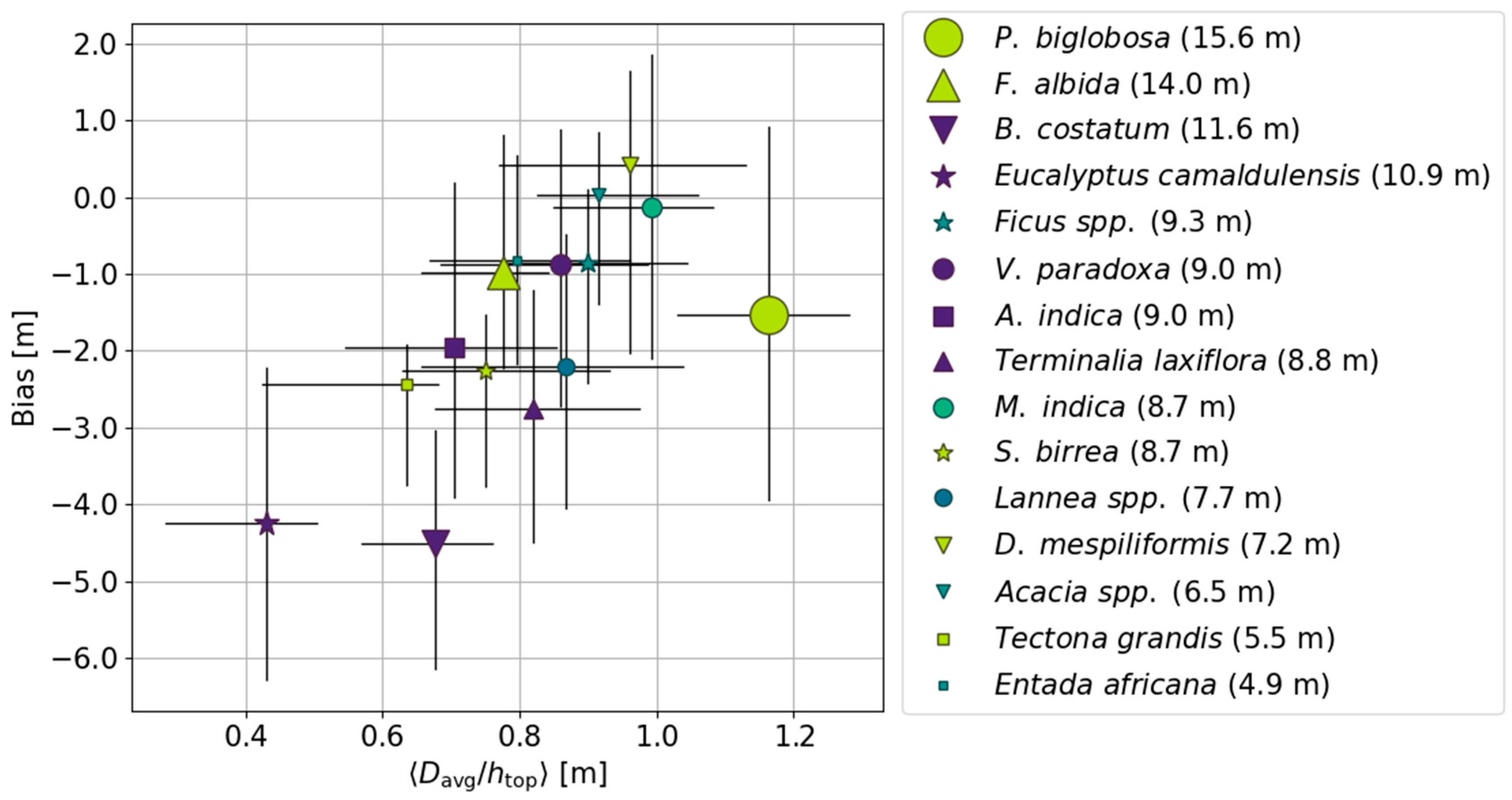
4.4. Effect of Species/Genera on Mean Canopy Elevation
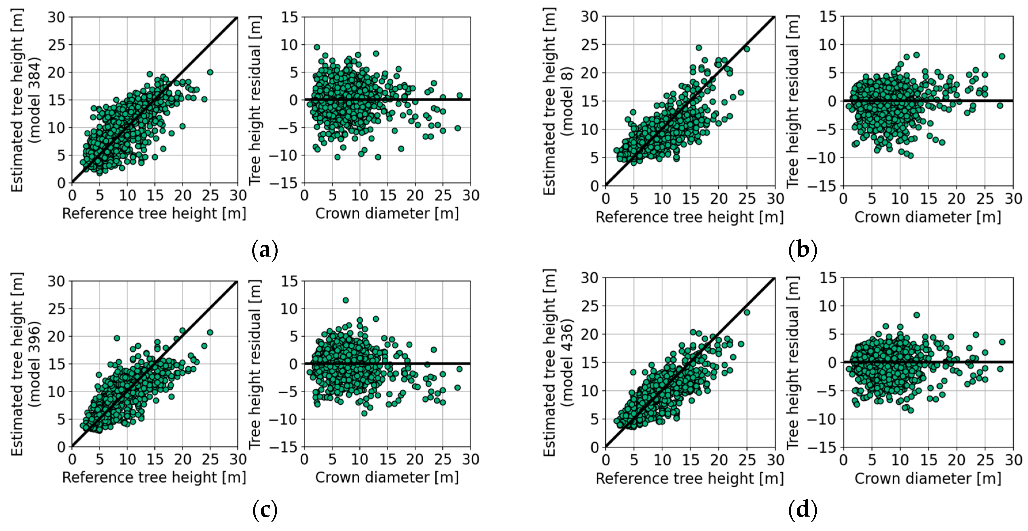
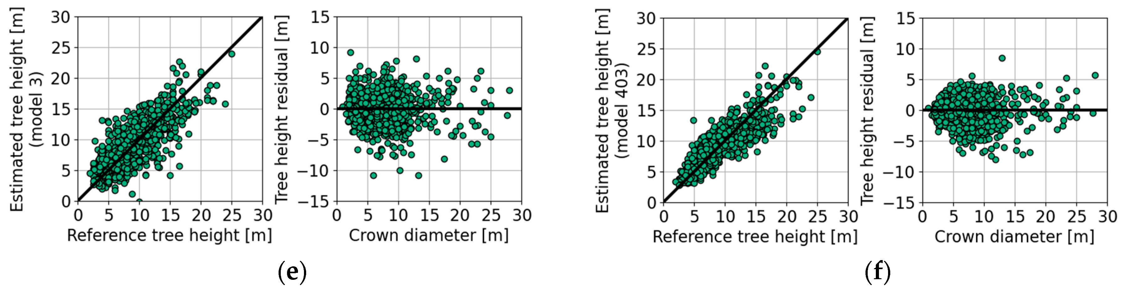
4.5. Tree Height Estimation with Empirical Models
5. Discussion
5.1. Tree Height Estimation Performance
5.2. Implementation Aspects and InSAR Data Considerations
6. Conclusions
Supplementary Materials
Author Contributions
Funding
Institutional Review Board Statement
Informed Consent Statement
Data Availability Statement
Acknowledgments
Conflicts of Interest
References
- Roupsard, O.; Audebert, A.; Ndour, A.P.; Clermont-Dauphin, C.; Agbohessou, Y.; Sanou, J.; Koala, J.; Faye, E.; Sambakhe, D.; Jourdan, C.; et al. How Far Does the Tree Affect the Crop in Agroforestry? New Spatial Analysis Methods in a Faidherbia Parkland. Agric. Ecosyst. Environ. 2020, 296, 106928. [Google Scholar] [CrossRef]
- Bargués Tobella, A.; Hasselquist, N.J.; Bazié, H.R.; Nyberg, G.; Laudon, H.; Bayala, J.; Ilstedt, U. Strategies Trees Use to Overcome Seasonal Water Limitation in an Agroforestry System in Semiarid West Africa. Ecohydrology 2017, 10, e1808. [Google Scholar] [CrossRef]
- Sanogo, K.; Binam, J.; Bayala, J.; Villamor, G.B.; Kalinganire, A.; Dodiomon, S. Farmers’ Perceptions of Climate Change Impacts on Ecosystem Services Delivery of Parklands in Southern Mali. Agrofor. Syst. 2017, 91, 345–361. [Google Scholar] [CrossRef]
- Ilstedt, U.; Tobella, A.B.; Bazié, H.R.; Bayala, J.; Verbeeten, E.; Nyberg, G.; Sanou, J.; Benegas, L.; Murdiyarso, D.; Laudon, H.; et al. Intermediate Tree Cover Can Maximize Groundwater Recharge in the Seasonally Dry Tropics. Sci. Rep. 2016, 6, 1–12. [Google Scholar] [CrossRef]
- Bayala, J.; Sanou, J.; Teklehaimanot, Z.; Kalinganire, A.; Ouédraogo, S. Parklands for Buffering Climate Risk and Sustaining Agricultural Production in the Sahel of West Africa. Curr. Opin. Environ. Sustain. 2014, 6, 28–34. [Google Scholar] [CrossRef] [Green Version]
- Karlson, M.; Ostwald, M.; Bayala, J.; Bazié, H.R.; Ouedraogo, A.S.; Soro, B.; Sanou, J.; Reese, H. The Potential of Sentinel-2 for Crop Production Estimation in a Smallholder Agroforestry Landscape, Burkina Faso. Front. Environ. Sci. 2020, 8, 85. [Google Scholar] [CrossRef]
- Bayala, J.; Sanou, J.; Teklehaimanot, Z.; Ouedraogo, S.J.; Kalinganire, A.; Coe, R.; Noordwijk, M. van Advances in Knowledge of Processes in Soil–Tree–Crop Interactions in Parkland Systems in the West African Sahel: A Review. Agric. Ecosyst. Environ. 2015, 205, 25–35. [Google Scholar] [CrossRef]
- Mechiche-Alami, A.; Abdi, A.M. Agricultural Productivity in Relation to Climate and Cropland Management in West Africa. Sci. Rep. 2020, 10, 3393. [Google Scholar] [CrossRef] [PubMed]
- Brandt, M.; Hiernaux, P.; Rasmussen, K.; Mbow, C.; Kergoat, L.; Tagesson, T.; Ibrahim, Y.Z.; Wélé, A.; Tucker, C.J.; Fensholt, R. Assessing Woody Vegetation Trends in Sahelian Drylands Using MODIS Based Seasonal Metrics. Remote Sens. Environ. 2016, 183, 215–225. [Google Scholar] [CrossRef] [Green Version]
- Papa, C.; Nzokou, P.; Mbow, C. Farmer Livelihood Strategies and Attitudes in Response to Climate Change in Agroforestry Systems in Kedougou, Senegal. Environ. Manag. 2020, 66, 218–231. [Google Scholar] [CrossRef]
- Karlson, M.; Ostwald, M. Remote Sensing of Vegetation in the Sudano-Sahelian Zone: A Literature Review from 1975 to 2014. J. Arid Environ. 2016, 124, 257–269. [Google Scholar] [CrossRef] [Green Version]
- Darkoh, M.B.K. Regional Perspectives on Agriculture and Biodiversity in the Drylands of Africa. J. Arid Environ. 2003, 54, 261–279. [Google Scholar] [CrossRef]
- Dardel, C.; Kergoat, L.; Hiernaux, P.; Mougin, E.; Grippa, M.; Tucker, C.J. Re-Greening Sahel: 30years of Remote Sensing Data and Field Observations (Mali, Niger). Remote Sens. Environ. 2014, 140, 350–364. [Google Scholar] [CrossRef]
- Heiskanen, J.; Liu, J.; Valbuena, R.; Aynekulu, E.; Packalen, P.; Pellikka, P. Remote Sensing Approach for Spatial Planning of Land Management Interventions in West African Savannas. J. Arid Environ. 2017, 140, 29–41. [Google Scholar] [CrossRef] [Green Version]
- Karlson, M.; Reese, H.; Ostwald, M. Tree Crown Mapping in Managed Woodlands (Parklands) of Semi-Arid West Africa Using WorldView-2 Imagery and Geographic Object Based Image Analysis. Sensors 2014, 14, 2643. [Google Scholar] [CrossRef]
- Lambert, M.-J.; Traoré, P.C.S.; Blaes, X.; Baret, P.; Defourny, P. Estimating Smallholder Crops Production at Village Level from Sentinel-2 Time Series in Mali’s Cotton Belt. Remote Sens. Environ. 2018, 216, 647–657. [Google Scholar] [CrossRef]
- Cho, M.A.; Mathieu, R.; Asner, G.P.; Naidoo, L.; van Aardt, J.; Ramoelo, A.; Debba, P.; Wessels, K.; Main, R.; Smit, I.P.J.; et al. Mapping Tree Species Composition in South African Savannas Using an Integrated Airborne Spectral and LiDAR System. Remote Sens. Environ. 2012, 125, 214–226. [Google Scholar] [CrossRef]
- Myeni, L.; Moeletsi, M.E.; Clulow, A.D. Present Status of Soil Moisture Estimation over the African Continent. J. Hydrol. Reg. Stud. 2019, 21, 14–24. [Google Scholar] [CrossRef]
- Forkuor, G.; Benewinde Zoungrana, J.-B.; Dimobe, K.; Ouattara, B.; Vadrevu, K.P.; Tondoh, J.E. Above-Ground Biomass Mapping in West African Dryland Forest Using Sentinel-1 and 2 Datasets—A Case Study. Remote Sens. Environ. 2020, 236, 111496. [Google Scholar] [CrossRef]
- Karlson, M. Remote Sensing of Woodland Structure and Composition in the Sudano-Sahelian Zone: Application of WorldView-2 and Landsat 8. Ph.D. Thesis, Linköping University, Linköping, Sweden, 2015. [Google Scholar]
- Ganz, S.; Käber, Y.; Adler, P. Measuring Tree Height with Remote Sensing—A Comparison of Photogrammetric and LiDAR Data with Different Field Measurements. Forests 2019, 10, 694. [Google Scholar] [CrossRef] [Green Version]
- Bamler, R.; Hartl, P. Synthetic Aperture Radar Interferometry. Inverse Probl. 1998, 14, R1–R54. [Google Scholar] [CrossRef]
- Farr, T.G.; Rosen, P.A.; Caro, E.; Crippen, R.; Duren, R.; Hensley, S.; Kobrick, M.; Paller, M.; Rodriguez, E.; Roth, L.; et al. The Shuttle Radar Topography Mission. Rev. Geophys. 2007, 45, 1–33. [Google Scholar] [CrossRef] [Green Version]
- Krieger, G.; Hajnsek, I.; Papathanassiou, K.P.; Younis, M.; Moreira, A. Interferometric Synthetic Aperture Radar (SAR) Missions Employing Formation Flying. Proc. IEEE 2010, 98, 816–843. [Google Scholar] [CrossRef] [Green Version]
- Rizzoli, P.; Martone, M.; Gonzalez, C.; Wecklich, C.; Borla Tridon, D.; Bräutigam, B.; Bachmann, M.; Schulze, D.; Fritz, T.; Huber, M.; et al. Generation and Performance Assessment of the Global TanDEM-X Digital Elevation Model. ISPRS J. Photogramm. Remote Sens. 2017, 132, 119–139. [Google Scholar] [CrossRef] [Green Version]
- Askne, J.I.H.; Fransson, J.E.S.; Santoro, M.; Soja, M.J.; Ulander, L.M.H. Model-Based Biomass Estimation of a Hemi-Boreal Forest from Multitemporal TanDEM-X Acquisitions. Remote Sens. 2013, 5, 5574–5597. [Google Scholar] [CrossRef] [Green Version]
- Solberg, S.; Astrup, R.; Breidenbach, J.; Nilsen, B.; Weydahl, D. Monitoring Spruce Volume and Biomass with InSAR Data from TanDEM-X. Remote Sens. Environ. 2013, 139, 60–67. [Google Scholar] [CrossRef]
- Kugler, F.; Schulze, D.; Hajnsek, I.; Pretzsch, H.; Papathanassiou, K.P. TanDEM-X Pol-InSAR Performance for Forest Height Estimation. IEEE Trans. Geosci. Remote Sens. 2014, 52, 6404–6422. [Google Scholar] [CrossRef]
- Soja, M.J.; Persson, H.; Ulander, L.M.H. Estimation of Forest Height and Canopy Density from a Single InSAR Correlation Coefficient. Geosci. Remote Sens. Lett. 2015, 12, 646–650. [Google Scholar] [CrossRef] [Green Version]
- Solberg, S.; May, J.; Bogren, W.; Breidenbach, J.; Torp, T.; Gizachew, B. Interferometric SAR DEMs for Forest Change in Uganda 2000–2012. Remote Sens. 2018, 10, 228. [Google Scholar] [CrossRef] [Green Version]
- Antonova, S.; Thiel, C.; Höfle, B.; Anders, K.; Helm, V.; Zwieback, S.; Marx, S.; Boike, J. Estimating Tree Height from TanDEM-X Data at the Northwestern Canadian Treeline. Remote Sens. Environ. 2019, 231, 111251. [Google Scholar] [CrossRef]
- Persson, H.; Olsson, H.; Soja, M.; Ulander, L.; Fransson, J. Experiences from Large-Scale Forest Mapping of Sweden Using TanDEM-X Data. Remote Sens. 2017, 9, 1253. [Google Scholar] [CrossRef] [Green Version]
- Lee, S.-K.; Fatoyinbo, T.E. TanDEM-X Pol-InSAR Inversion for Mangrove Canopy Height Estimation. IEEE J. Sel. Top. Appl. Earth Obs. Remote Sens. 2015, 8, 3608–3618. [Google Scholar] [CrossRef]
- Treuhaft, R.; Gonzalves, F.; dos Santos, J.R.; Keller, M.; Palace, M.; Madsen, S.N.; Sullivan, F.; Graca, P.M.L.A. Tropical-Forest Biomass Estimation at X-Band From the Spaceborne TanDEM-X Interferometer. IEEE Geosci. Remote Sens. Lett. 2015, 12, 239–243. [Google Scholar] [CrossRef] [Green Version]
- Krieger, G.; Moreira, A.; Fiedler, H.; Hajnsek, I.; Werner, M.; Younis, M.; Zink, M. TanDEM-X: A Satellite Formation for High-Resolution SAR Interferometry. IEEE Trans. Geosci. Remote Sens. 2007, 45, 3317–3341. [Google Scholar] [CrossRef] [Green Version]
- Kellndorfer, J.; Walker, W.; Pierce, L.; Dobson, C.; Fites, J.A.; Hunsaker, C.; Vona, J.; Clutter, M. Vegetation Height Estimation from Shuttle Radar Topography Mission and National Elevation Datasets. Remote Sens. Environ. 2004, 93, 339–358. [Google Scholar] [CrossRef]
- Hirt, C.; Filmer, M.S.; Featherstone, W.E. Comparison and Validation of the Recent Freely Available ASTER-GDEM Ver1, SRTM Ver4.1 and GEODATA DEM-9S Ver3 Digital Elevation Models over Australia. Aust. J. Earth Sci. 2010, 57, 337–347. [Google Scholar] [CrossRef] [Green Version]
- Solberg, S.; Astrup, R.; Gobakken, T.; Naesset, E.; Weydahl, D.J. Estimating Spruce and Pine Biomass with Interferometric X-Band SAR. Remote Sens. Environ. 2010, 114, 2353–2360. [Google Scholar] [CrossRef]
- Dubayah, R.; Blair, J.B.; Goetz, S.; Fatoyinbo, L.; Hansen, M.; Healey, S.; Hofton, M.; Hurtt, G.; Kellner, J.; Luthcke, S.; et al. The Global Ecosystem Dynamics Investigation: High-Resolution Laser Ranging of the Earth’s Forests and Topography. Sci. Remote Sens. 2020, 1, 100002. [Google Scholar] [CrossRef]
- Curlander, J.C.; McDonough, R.N. Synthetic Aperture Radar: Systems and Signal. Processing; John Wiley & Sons Inc.: Hoboken, NJ, USA, 1992. [Google Scholar]
- Cloude, S.R.; Papathanassiou, K.P. Polarimetric SAR Interferometry. IEEE Trans. Geosci. Remote Sens. 1998, 36, 1551–1565. [Google Scholar] [CrossRef]
- Soja, M.J.; Askne, J.I.H.; Ulander, L.M.H. Estimation of Boreal Forest Properties from TanDEM-X Data Using Inversion of the Interferometric Water Cloud Model. IEEE Geosci. Remote Sens. Lett. 2017, 14, 997–1001. [Google Scholar] [CrossRef]
- Soja, M.J.; Persson, H.J.; Ulander, L.M.H. Estimation of Forest Biomass from Two-Level Model Inversion of Single-Pass InSAR Data. IEEE Trans. Geosci. Remote Sens. 2015, 53, 5083–5099. [Google Scholar] [CrossRef] [Green Version]
- Soja, M.J.; Persson, H.J.; Ulander, L.M.H. Modeling and Detection of Deforestation and Forest Growth in Multitemporal TanDEM-X Data. IEEE J. Sel. Top. Appl. Earth Obs. Remote Sens. 2018, 11, 3548–3563. [Google Scholar] [CrossRef]
- Zebker, H.A.; Villasenor, J. Decorrelation in Interferometric Radar Echoes. IEEE Trans. Geosci. Remote Sens. 1992, 30, 950–959. [Google Scholar] [CrossRef] [Green Version]
- Bazié, H.R.; Bayala, J.; Zombré, G.; Sanou, J.; Ilstedt, U. Separating Competition-Related Factors Limiting Crop Performance in an Agroforestry Parkland System in Burkina Faso. Agrofor. Syst. 2012, 84. [Google Scholar] [CrossRef]
- Bayala, J.; Teklehaimanot, Z.; Ouedraogo, S.J. Millet Production under Pruned Tree Crowns in a Parkland System in Burkina Faso. Agrofor. Syst. 2002, 54, 203–214. [Google Scholar] [CrossRef]
- Karlson, M.; Ostwald, M.; Reese, H.; Sanou, J.; Tankoano, B.; Mattsson, E. Mapping Tree Canopy Cover and Aboveground Biomass in Sudano-Sahelian Woodlands Using Landsat 8 and Random Forest. Remote Sens. 2015, 7, 10017–10041. [Google Scholar] [CrossRef] [Green Version]
- Boffa, J.M. Agroforestry Parkland in Sub-Saharan Africa FAO Conservation Guide 34; United Nations Food and Agricultural Organization: Rome, Italy, 1999. [Google Scholar]
- Weather Underground Ouagadougou, Kadiogo, Burkina Faso Weather History. Available online: https://www.wunderground.com/history/daily/bf/ouagadougou/DFFD (accessed on 31 August 2020).
- GAMMA. GAMMA Remote Sensing. Available online: http://www.gamma-rs.ch (accessed on 7 September 2020).
- Duque, S.; Balss, U.; Rossi, C.; Fritz, T.; Balzer, W. TanDEM-X Payload Ground Segment, CoSSC Generation and Interferometric Considerations; Remote Sensing Technology Institute, German Aerospace Center (DLR): Köln, Germany, 2012. [Google Scholar]
- Airbus Defence & Space. Radiometric Calibration of TerraSAR-X Data: Beta Naught and Sigma Naught Coefficient Calculation; AIRBUS: Leiden, The Netherlands, 2014. [Google Scholar]
- Kass, M.; Witkin, A.; Terzopoulos, D. Snakes: Active Contour Models. Int. J. Comput. Vis. 1988, 1, 321–331. [Google Scholar] [CrossRef]
- Elmqvist, M. Ground Surface Estimation from Airborne Laser Scanning Data Using Active Shape Models. Int. Arch. Photogramm. Remote Sens. Spat. Inf. Sci. 2002, 34, 114–118. [Google Scholar]
- Nocedal, J.; Wright, S.J. Numerical Optimization, 2nd ed.; Springer Series in Operations Research; Springer: New York, NY, USA, 2006; ISBN 978-0-387-30303-1. [Google Scholar]
- St-Onge, B.; Grandin, S. Estimating the Height and Basal Area at Individual Tree and Plot Levels in Canadian Subarctic Lichen Woodlands Using Stereo WorldView-3 Images. Remote Sens. 2019, 11, 248. [Google Scholar] [CrossRef] [Green Version]
- Khalefa, E.; Smit, I.P.J.; Nickless, A.; Archibald, S.; Comber, A.; Balzter, H. Retrieval of Savanna Vegetation Canopy Height from ICESat-GLAS Spaceborne LiDAR With Terrain Correction. IEEE Geosci. Remote Sens. Lett. 2013, 10, 1439–1443. [Google Scholar] [CrossRef] [Green Version]
- Kumar, P.; Krishna, A.P. InSAR-Based Tree Height Estimation of Hilly Forest Using Multitemporal Radarsat-1 and Sentinel-1 SAR Data. IEEE J. Sel. Top. Appl. Earth Obs. Remote Sens. 2019, 12, 5147–5152. [Google Scholar] [CrossRef]
- Fassnacht, F.E.; Latifi, H.; Stereńczak, K.; Modzelewska, A.; Lefsky, M.; Waser, L.T.; Straub, C.; Ghosh, A. Review of Studies on Tree Species Classification from Remotely Sensed Data. Remote Sens. Environ. 2016, 186, 64–87. [Google Scholar] [CrossRef]
- Karlson, M.; Ostwald, M.; Reese, H.; Bazié, H.R.; Tankoano, B. Assessing the Potential of Multi-Seasonal WorldView-2 Imagery for Mapping West African Agroforestry Tree Species. Int. J. Appl. Earth Obs. Geoinf. 2016, 50, 80–88. [Google Scholar] [CrossRef]
- Quegan, S.; Le Toan, T.; Chave, J.; Dall, J.; Exbrayat, J.-F.; Minh, D.H.T.; Lomas, M.; D’Alessandro, M.M.; Paillou, P.; Papathanassiou, K.; et al. The European Space Agency BIOMASS Mission: Measuring Forest above-Ground Biomass from Space. Remote Sens. Environ. 2019, 227, 44–60. [Google Scholar] [CrossRef] [Green Version]


| Metric | Explanation |
|---|---|
| In situ-measured tree properties | |
| Top-of-canopy height | |
| Stem diameter at breast height (1.3 m) | |
| Crown diameter averaged across two perpendicular directions | |
| Raster data | |
| DTM | Digital terrain model (estimated ground elevation above a reference surface) |
| DEM | Digital elevation model (interferometric height above a reference surface) |
| Phase height (DEM elevation above the DTM) | |
| Mean canopy elevation (model-based estimate of canopy elevation above the DTM) | |
| Tree height estimates | |
| within the extent of the crown for a single tree | |
| within the extent of the crown for a single tree | |
| (shifted by a constant so that a regression line for all trees goes through zero) | |
| Calibrated (shifted by a constant so that a regression line for all trees goes through zero) | |
| Top-of-canopy height estimate from an empirical model | |
| Model parameters | |
| Distance between ground and vegetation levels in the two-level model (TLM) | |
| Dates | Used Trees (Total) | ||||||
|---|---|---|---|---|---|---|---|
| Min | Mean | Max | Min | Mean | Max | ||
| October–December 2012 | 401 (1125) | 2.5 | 7.0 | 20.0 | 1.0 | 6.0 | 28.0 |
| October 2017 | 241 (637) | 2.0 | 9.9 | 25.0 | 2.0 | 9.3 | 27.7 |
| June 2018 | 273 (321) | 3.5 | 11.1 | 23.9 | 2.0 | 8.2 | 25.0 |
| All | 915 (2083) | 2.0 | 9.0 | 25.0 | 1.0 | 7.5 | 28.0 |
| Date | Time (UTC): | Orbit | Pol | HOA (m) | Res (m) | Temp (°C) | ||||
|---|---|---|---|---|---|---|---|---|---|---|
| No | Dir | grg | az | |||||||
| 24 January 2018 | 6:03 AM | 63 | dsc | 191 | 32 | HH | 39 | 2.1 | 1.1 | 16 |
| 26 February 2018 | 47 | 24 | ||||||||
| 31 March 2018 | 55 | 25 | ||||||||
| 9 February 2018 | 6:09 PM | 147 | asc | 349 | 25 | 49 | 2.8 | 1.1 | 28 | |
| 20 February 2018 | 59 | 36 | ||||||||
| 25 March 2018 | 79 | 33 | ||||||||
| 5 April 2018 | 87 | 37 | ||||||||
| Orbit Direction: | Ascending | Descending | Combined | |||||||||
|---|---|---|---|---|---|---|---|---|---|---|---|---|
| Tree height group: | <8 | 8–16 | >16 | All | <8 | 8–16 | >16 | All | <8 | 8–16 | >16 | All |
| −0.1 | 1.0 | 6.0 | 0.4 | 0.2 | −0.5 | −3.9 | −0.2 | −0.0 | 0.3 | 1.0 | 0.1 | |
| 0.2 | 0.2 | 0.9 | 0.2 | 0.0 | −0.1 | −0.5 | −0.1 | 0.0 | −0.1 | 1.3 | 0.0 | |
| 1.5 | 2.8 | 4.1 | 2.3 | 1.5 | 3.0 | 5.1 | 2.4 | 1.5 | 2.9 | 7.3 | 2.3 | |
| 2.4 | 2.9 | 3.4 | 2.6 | 1.5 | 2.8 | 4.1 | 2.2 | 1.6 | 2.8 | 3.3 | 2.1 | |
| Mean canopy elevation () | ||||||||||||
| Orbit direction: | Ascending | Descending | Combined | |||||||||
| Tree height group: | <8 | 8–16 | >16 | All | <8 | 8–16 | >16 | All | <8 | 8–16 | >16 | All |
| −0.2 | −1.2 | −0.6 | −0.6 | 0.1 | 1.5 | 2.8 | 0.6 | −0.0 | 0.2 | 0.4 | 0.1 | |
| 0.2 | 0.6 | −0.2 | 0.3 | 0.1 | 0.6 | 2.2 | 0.4 | 0.1 | 0.7 | 0.5 | 0.3 | |
| 1.6 | 2.5 | 5.5 | 2.2 | 1.4 | 2.8 | 3.7 | 2.2 | 1.5 | 2.5 | 3.5 | 2.0 | |
| 1.6 | 2.8 | 3.3 | 2.2 | 1.6 | 2.8 | 3.9 | 2.2 | 1.5 | 2.7 | 3.1 | 2.1 | |
| Figure | Tree Height Estimate | N | S | rp (%) | Bias (m) | SE (m) | ||||||
|---|---|---|---|---|---|---|---|---|---|---|---|---|
| <8 | 8–16 | >16 | All | <8 | 8–16 | >16 | All | |||||
| Figure 7a | 915 | 15 | 75 | −0.7 | −1.5 | −3.9 | −1.3 | 2.6 | 3.1 | 2.9 | 3.0 | |
| Figure 7b | 915 | 15 | 73 | −2.7 | −4.2 | −7.7 | −3.7 | 2.2 | 2.8 | 2.9 | 2.9 | |
| Figure | Model Properties | Bias (m) | SE (m) | ||||||||||
|---|---|---|---|---|---|---|---|---|---|---|---|---|---|
| Formula | <8 | 8–16 | >16 | All | <8 | 8–16 | >16 | All | |||||
| Empirical models and species-independent parameters | |||||||||||||
| Figure 10a | 1 | 915 | 15 | 75 | 0.8 | −0.3 | −3.0 | 0.0 | 2.4 | 2.9 | 2.8 | 2.8 | |
| Figure 10b | 2 | 915 | 15 | 76 | 1.5 | −1.0 | −3.3 | 0.0 | 1.3 | 2.4 | 4.0 | 2.6 | |
| Figure 10c | 1 | 915 | 15 | 79 | 1.0 | −0.4 | −4.2 | 0.0 | 1.8 | 2.5 | 2.2 | 2.5 | |
| Figure 10d | 3 | 915 | 15 | 82 | 1.1 | −0.6 | −3.5 | 0.0 | 1.4 | 2.3 | 2.6 | 2.3 | |
| Empirical models and species-specific parameters | |||||||||||||
| Figure 10e | 16 | 853 | 8 | 79 | 0.7 | −0.3 | −2.4 | 0.0 | 2.2 | 2.7 | 3.2 | 2.6 | |
| Figure 10f | 16 | 853 | 8 | 87 | 0.7 | −0.3 | −3.0 | 0.0 | 1.4 | 2.0 | 3.0 | 2.0 | |
Publisher’s Note: MDPI stays neutral with regard to jurisdictional claims in published maps and institutional affiliations. |
© 2021 by the authors. Licensee MDPI, Basel, Switzerland. This article is an open access article distributed under the terms and conditions of the Creative Commons Attribution (CC BY) license (https://creativecommons.org/licenses/by/4.0/).
Share and Cite
Soja, M.J.; Karlson, M.; Bayala, J.; Bazié, H.R.; Sanou, J.; Tankoano, B.; Eriksson, L.E.B.; Reese, H.; Ostwald, M.; Ulander, L.M.H. Mapping Tree Height in Burkina Faso Parklands with TanDEM-X. Remote Sens. 2021, 13, 2747. https://0-doi-org.brum.beds.ac.uk/10.3390/rs13142747
Soja MJ, Karlson M, Bayala J, Bazié HR, Sanou J, Tankoano B, Eriksson LEB, Reese H, Ostwald M, Ulander LMH. Mapping Tree Height in Burkina Faso Parklands with TanDEM-X. Remote Sensing. 2021; 13(14):2747. https://0-doi-org.brum.beds.ac.uk/10.3390/rs13142747
Chicago/Turabian StyleSoja, Maciej J., Martin Karlson, Jules Bayala, Hugues R. Bazié, Josias Sanou, Boalidioa Tankoano, Leif E. B. Eriksson, Heather Reese, Madelene Ostwald, and Lars M. H. Ulander. 2021. "Mapping Tree Height in Burkina Faso Parklands with TanDEM-X" Remote Sensing 13, no. 14: 2747. https://0-doi-org.brum.beds.ac.uk/10.3390/rs13142747