
Aboveground Biomass Mapping of Crops Supported by Improved CASA Model and Sentinel-2 Multispectral Imagery


1
Key Laboratory of Geospatial Technology for the Middle and Lower Yellow River Regions (Henan University), Ministry of Education, Kaifeng 475004, China
2
College of Geography and Environmental Science, Henan University, Kaifeng 475004, China
3
State Key Laboratory of Remote Sensing Science, Aerospace Information Research Institute, Chinese Academy of Sciences, Beijing 100101, China
*
Author to whom correspondence should be addressed.
†
These authors contributed equally to this work.
Remote Sens. 2021, 13(14), 2755; https://0-doi-org.brum.beds.ac.uk/10.3390/rs13142755
Submission received: 19 June 2021
/
Revised: 8 July 2021
/
Accepted: 11 July 2021
/
Published: 13 July 2021
(This article belongs to the Special Issue Earth Observations and Crop Models for Sustainable Agricultural Management: Part II)
Abstract
:The net primary productivity (NPP) and aboveground biomass mapping of crops based on remote sensing technology are not only conducive to understanding the growth and development of crops but can also be used to monitor timely agricultural information, thereby providing effective decision making for agricultural production management. To solve the saturation problem of the NDVI in the aboveground biomass mapping of crops, the original CASA model was improved using narrow-band red-edge information, which is sensitive to vegetation chlorophyll variation, and the fraction of photosynthetically active radiation (FPAR), NPP, and aboveground biomass of winter wheat and maize were mapped in the main growing seasons. Moreover, in this study, we deeply analyzed the seasonal change trends of crops’ biophysical parameters in terms of the NDVI, FPAR, actual light use efficiency (LUE), and their influence on aboveground biomass. Finally, to analyze the uncertainty of the aboveground biomass mapping of crops, we further discussed the inversion differences of FPAR with different vegetation indices. The results demonstrated that the inversion accuracies of the FPAR of the red-edge normalized vegetation index () and red-edge simple ratio vegetation index () were higher than those of the original CASA model. Compared with the reference data, the accuracy of aboveground biomass estimated by the improved CASA model was 0.73 and 0.70, respectively, which was 0.21 and 0.13 higher than that of the original CASA model. In addition, the analysis of the FPAR inversions of different vegetation indices showed that the inversion accuracies of the red-edge vegetation indices and were higher than those of the other vegetation indices, which confirmed that the vegetation indices involving red-edge information can more effectively retrieve FPAR and aboveground biomass of crops.

1. Introduction
Remote sensing technology is widely used in crop yield prediction [1,2,3,4,5], identification mapping [6,7,8], aboveground biomass estimation [9,10], LAI inversion [11,12,13,14], and many other fields of agricultural production, and it has always been the focus of attention in studies of crop biomass [2,15,16]. Moreover, the use of remote sensing data during crop growth periods to estimate crop biomass quickly and accurately is an unavoidable key issue for agricultural remote sensing research.
At present, there are two main methods for estimation of crops biomass with remote sensing: vegetation index regression methods and productivity models [9]. Generally, direct modeling using vegetation indices and measured crop biomass can easily and quickly estimate aboveground biomass of crops.
With the development of multispectral sensors, many researchers have found that the red-edge vegetation indices are more sensitive than wide-band vegetation indices. Zheng et al. [17] established a fitting model for predicted winter wheat biomass, with the NDVI, enhanced vegetation index (EVI), and chlorophyll red-edge index (CIre). Their work showed that the CIre had the best correlation with the measured biomass. Kross et al. [18] used multispectral RapidEye data with a high spatial resolution to estimate the leaf area index (LAI) and biomass of corn and soybeans. They believed that the SRred-edge performed well in terms of its ability to estimate the total biomass of corn. Frampton et al. [19] constructed two new indices S2REP (sentinel-2 red edge position) and IRECI (red-edge chlorophyll index) using the red edge band of sentinel-2 data. They reported that S2REP was more suitable for retrieving chlorophyll concentration, while the performance of IREC was still better, even when the saturation point was exceeded.
Various vegetation index regression models were used to accurately estimate the vegetation biomass in previous research. However, identifying suitable variables for developing a vegetation regression model is usually difficult and time-consuming because many potential variables should be used. Aboveground biomass is a comprehensive parameter related to sophisticated factors, such as canopy structure, solar radiation, and photosynthetically active radiation [9]. In addition to the more commonly used vegetation index regression methods, models based on NPP are also increasingly applied to biomass mapping. NPP models are usually divided into three types: climate-related models, physiological and ecological-related models, and light use efficiency models [20]. Generally, light use efficiency models (CASA, GLO-PEM, etc.) are easy to combine with remote sensing data. Therefore, increasing studies have applied this model to estimate the NPP, biomass of vegetation and crops at global or national scales. In 1972, when Monteith [21] analyzed the relationship between the productivity of tropical ecosystems and solar radiation, he proposed, for the first time, that the productivity of plants depends on the solar radiation intercepted by the leaves, the photosynthetic rate of the leaves, and other photochemical processes. According to the theory proposed by Monteith, Potter et al. [22] used the CASA model combined with AVHRR image data to simulate a global scale model of the carbon sequestration cycle model and biomass of vegetation. In recent years, the CASA model has been widely used in terrestrial ecosystem research, NPP research, biomass estimation, etc. Bao et al. [23] proposed an improved LSWI-CASA that simplified the CASA model’s estimation process and estimated the NPP of the Mongolian Plateau. The results illustrated that the method improved the accuracy of NPP estimation. Using 30 m resolution HJ-AB images, Liu [24] applied the CASA model to the estimate the biomass and yield of winter wheat. Compared with the measured data, the CASA model had higher accuracy in crop biomass and yield estimation. Tao [25] comprehensively compared the performance of the CASA and GLO-PEM models in estimating the NPP of Chinese maize. He confirmed that the CASA model had a better estimation accuracy than that of the GLO-PEM when the crop planting density was high. On the contrary, the estimation accuracy of GLO-PEM model was higher than that of the CASA model.
Overall, the aboveground biomass mapping of crops is an essential issue in the field of agricultural remote sensing. The vegetation index regression methods can quickly obtain crop biomass information, but these methods require large amounts of measured data, and their performance is not accurate when applied at global or national scales. In addition, these methods only fit the dry weight of the crops at mature stage with vegetation indices and cannot reflect the growth and mechanism of the crops during the growing season. As an NPP estimation model based on vegetation photosynthetic efficiency, CASA has been increasingly applied to NPP estimation and carbon storage research for global or national vegetation, and it has achieved good results. However, currently, there are few studies on the use of the CASA model to map high-resolution crop biomass on a small irrigation scale. By applying this model to small areas, high-resolution biomass mapping will help expand the usage of the CASA model. In addition, much of research has demonstrated that the wide-band vegetation index, NDVI, is easily saturated in areas of dense vegetation and affects the inversion of plant biophysical parameters [11,15,17]. The wide-band vegetation index, NDVI, is used to retrieve the key parameter, FPAR, in the original CASA, which affects the estimation accuracy of the FPAR and biomass to a certain extent. Based on the above problems, we utilized red-edge vegetation indices, which are sensitive to changes in vegetation chlorophyll variation, for the FPAR inversion, and applied the results to the estimation of NPP and aboveground biomass of crops in a small irrigation scale region.
2. Materials and Methods
2.1. Study Area
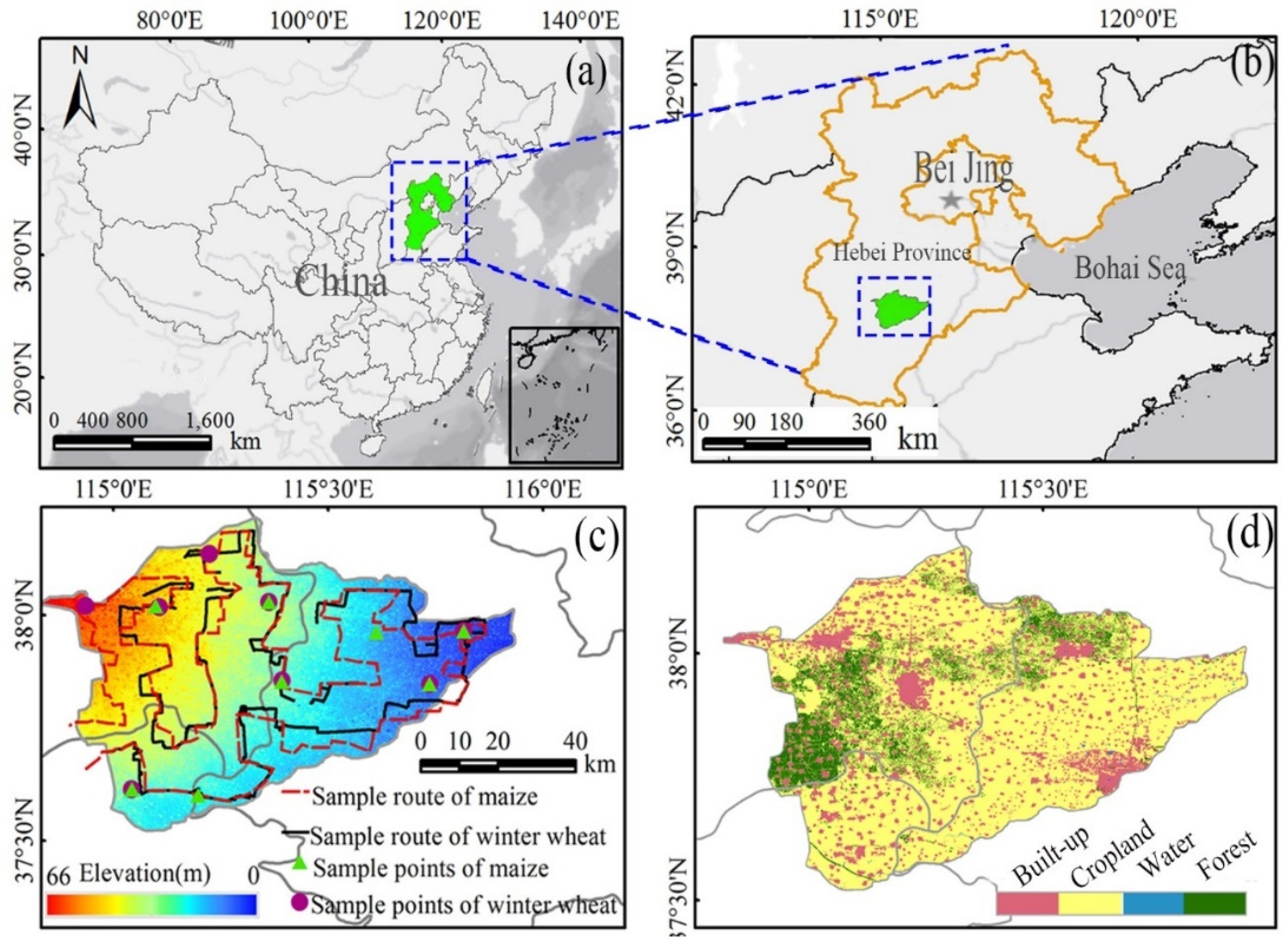
The Shijin irrigation area (115.08E, 38.02N), Hebei Province, is located in the Heibei province, and it is an important grain production area in China (Figure 1a,b). The land use in this irrigation area is mainly cropland (69%), with a small amount of built-up (18%), forest (11%), and water (2%) (Figure 1d). The easternmost part is close to the Bohai Sea, and the southeastern part is close to the Haihe River. The irrigation area is flat, with an altitude range of 0–60 m, and a total area of 14,933 km2. Irrigation facilities are complete, which provides a large amount of water resources for agricultural production. The irrigation area has a continental monsoon climate. The total amount of precipitation in the irrigation area is about 488 mm, the annual frost-free period is 190–200 days, the annual sunshine hours are about 2626 h, and the accumulated temperature above zero is 4600–5000 °C. The good climatic conditions in the irrigation area provide sufficient water and heat resources for the winter wheat and summer corn rotation system, and they are beneficial to the development of characteristic orchards, such as apple and pear orchards, in the irrigation area. In 2019, we made a field survey route for the irrigation area and conducted field survey for the main crops to obtain the aboveground biomass data of winter wheat and summer maize (Figure 1c).
2.2. Datasets and Processing
2.2.1. Meteorological Data
The meteorological data came from the Dataset of Daily Values of Climate Data V3.0 (http://www.cma.gov.cn/2011qxfw/2011qsjgx/, accessed on 8 August 2020) provided by the China Meteorological Data Service Center. The dataset contains the meteorological elements, such as temperature, precipitation, evaporation, and sunshine hours, of 699 basic weather stations across the country. In addition, to obtain accurate solar radiation data in crop growing season, we simulated the meteorological data needed for the study using Angstrom model [26,27] based on sunshine hour data (listed in Table 1). In order to process the original data, in this study, we used python to perform unit conversion and default value processing for the temperature and sunshine hour data that were used. Finally, the nearest meteorological station in the Shijin irrigation area was selected as the meteorological element required for the research.
2.2.2. Remote Sensing Data
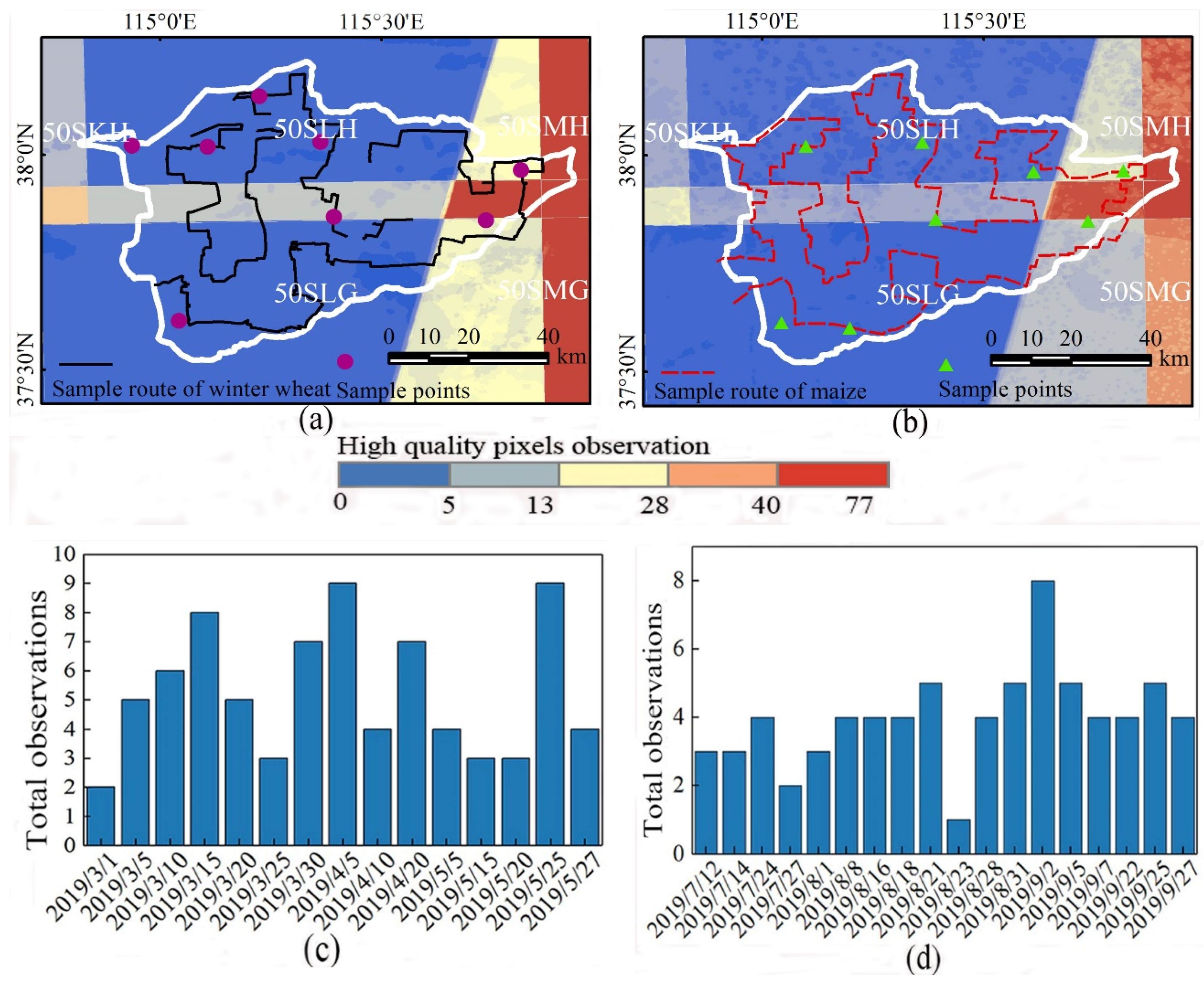
Sentinel-2 satellites have high-resolution and multispectral information, and they include 13 multispectral bands (Table 1). Among them are four 10 m resolution bands, six 20 m bands, and three 60 m bands, with an orbital width of 290 km [28]. As Sentinel-2 has multiple narrow bands in the visible and near-infrared ranges, it plays an important role in land use/cover [29], vegetation growth [30], water cover [31], and crop mapping [32]. Based on the Google Earth Engine [33,34] (https://earthengine.google.com/, accessed on 6 November 2020) remote sensing big data platform, we filtered many high-quality images (cloud coverage < 20%). We obtained 133 Sentinel-2 multispectral images during the key growing seasons of the two crops. Among them, 61 were in the key growing season of winter wheat and 72 were in the main growing season of summer maize (Figure 2).
MCD15A3H LAI/FPAR data product with a resolution of 4 days and 500 m in the main growing season of winter wheat and summer maize was selected for this study (Table 1). The MODIS Terra and Aqua images of this product were corrected for surface reflectance and atmospheric effect. The main inversion algorithm and backup algorithm were used to select the highest-quality image pixels to generate LAI/FPAR product [35]. Among them, the main algorithm used the biome/canopy model to retrieve the LAI/FPAR, and it searched for all possible values of the LAI/FPAR, according to the specific solar angle of view, the bidirectional reflection coefficient, and the type of biome. If specific pixels were provided for modeling, the vegetation index was used to fit the LAI/FPAR, and the LUT was generated to obtain the LAI/FPAR value. The LAI/FPAR provided by MODIS product has a high accuracy and is widely used in the estimation of vegetation LAI, FPAR, and biomass [36].
2.2.3. Measured Field Data
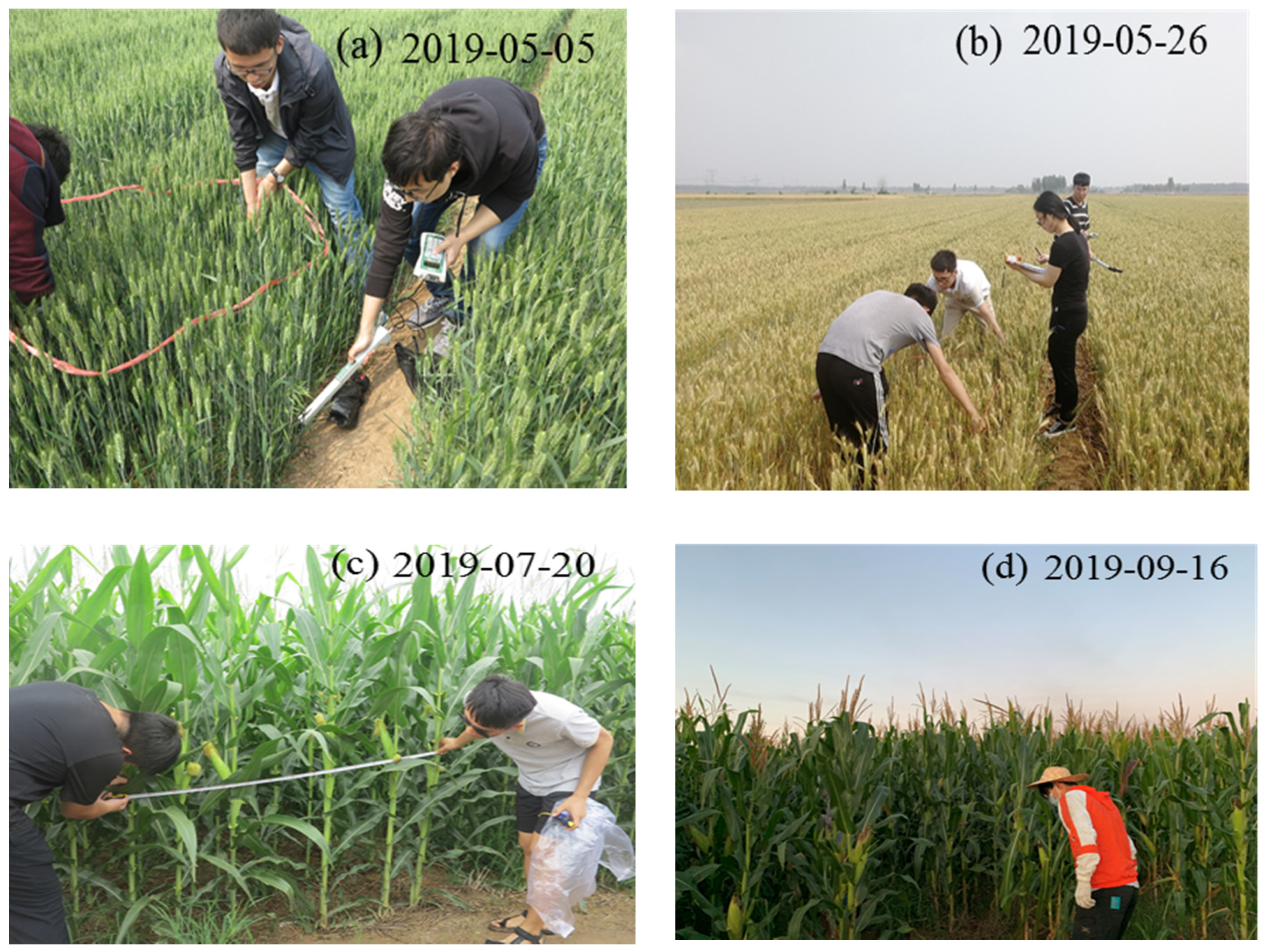
The measured data were obtained from field measurements of winter wheat (March to May) and summer maize (July to September) during the main observation period (Figure 3). Eight sampling points were set for each crop survey, and all of the sampling points were evenly distributed in the whole study area. Before sampling, the row density and column density of the crops were measured to find the planting density information of the crops per square meter. As it was difficult to obtain the whole crop, only the part above the root of the crop was taken when sampling. In order to obtain the dry weight data of the crop, it was necessary to dry the winter wheat and maize. For winter wheat, we set the oven temperature to 105 °C for 1 h, and then dried it at a constant temperature of 80 °C for 24 h. For summer maize, we set the temperature to 105 °C for 3 h, and then dried it at a constant temperature of 80 °C for 48 h. After the dried crop was obtained, the crop dry weight per unit area was obtained (listed in Table 2).
2.3. Methods
2.3.1. Processing Flow of the Original CASA Model
According to the research of Potter et al. [22], the CASA model involves two important variables: one is the photosynthetically active radiation intercepted by the green vegetation canopy, and the other is light use efficiency (Equations (1)–(4) [22,37]). The calculation of photosynthetically active radiation involves the fraction of photosynthetically active radiation absorbed by the vegetation canopy, and related studies have proved that there is a significant linear relationship between the photosynthetically active radiation and the vegetation index, so the vegetation index can be used for the calculations. The calculation of the light use efficiency involves factors such as temperature and water stress.
where NPP is the net primary productivity of the vegetation. APAR is the photosynthetically active radiation absorbed by the vegetation canopy. LUE is the actual light use efficiency of the plants. PAR is the photosynthetically active radiation. FPAR is the photosynthetically active radiation absorption proportion. is the maximum LUE, and ,, and are scalars representing environmental stressors that reduce LUE [38,39]. According to this formula, the FPAR in the original CASA model is a function of the NDVI, so this also means that the FPAR may be underestimated in dense vegetation areas.
2.3.2. Vegetation Indices
The red-edge band is an essential variable for retrieving the LAI, FPAR, etc., and it plays an important role in biomass estimation. To solve the saturation problem of the NDVI in the biomass mapping of crops, this study incorporates narrow-band red-edge information from Sentinel-2 into the inversion of the FPAR in Table 3. Besides, in order to analyze the inversion differences of FPAR with different vegetation indices, we further obtained the inversions accuracies of FPAR of the red-edge indices and non-red-edge indices including NDVI, SR, MSR, EVI, , and (Table 4). The differences in the FPAR were derived by analyzing different vegetation indices to improve the accuracy of FPAR inversion.
2.3.3. Conversion of NPP into Aboveground Biomass
Much of the research in aboveground biomass mapping has shown that the nature of the accumulation of NPP in green plants reflects the relationship between the dry matter formed through the photosynthesis of the vegetation and carbon fixation. With the development of green plant stalks and leaves, their photosynthetic capacity is not enhanced, and the carbon sequestration capacity is continuously improved. Some studies have proposed NPP-driven biomass inversion models on this theoretical basis [47,48]. They believe that there is a significant linear relationship between plant biomass and accumulated NPP that is affected by the root-to-shoot ratio and C ratio.
where B refers to the biomass of the plant. NPP is the net primary productivity accumulated in growth stages. α is the ratio of the aboveground biomass of the plant to the whole plant. β is the C ratio of a crop. It can be seen in Equation (12) that there is a simple linear relationship between plant biomass and accumulated NPP. When the plant root-to-shoot ratio and C content parameters are determined, the NPP can be converted into aboveground biomass.
2.3.4. Accuracy Assessment
The retrieval accuracy and biomass estimation accuracy of the two models are described and compared using the coefficient of determination (R2) and root mean square error (RMSE), as shown in Equations (13) and (14).
where represents the number of variables; represents the predicted value; represents the field-measured value; is the average of the field-measured values.
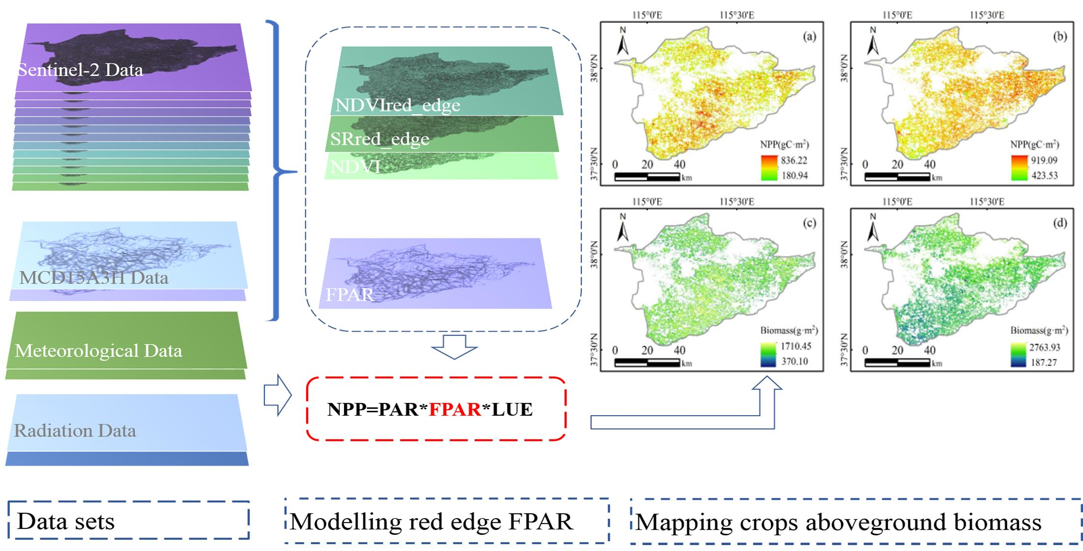
2.4. Workflow
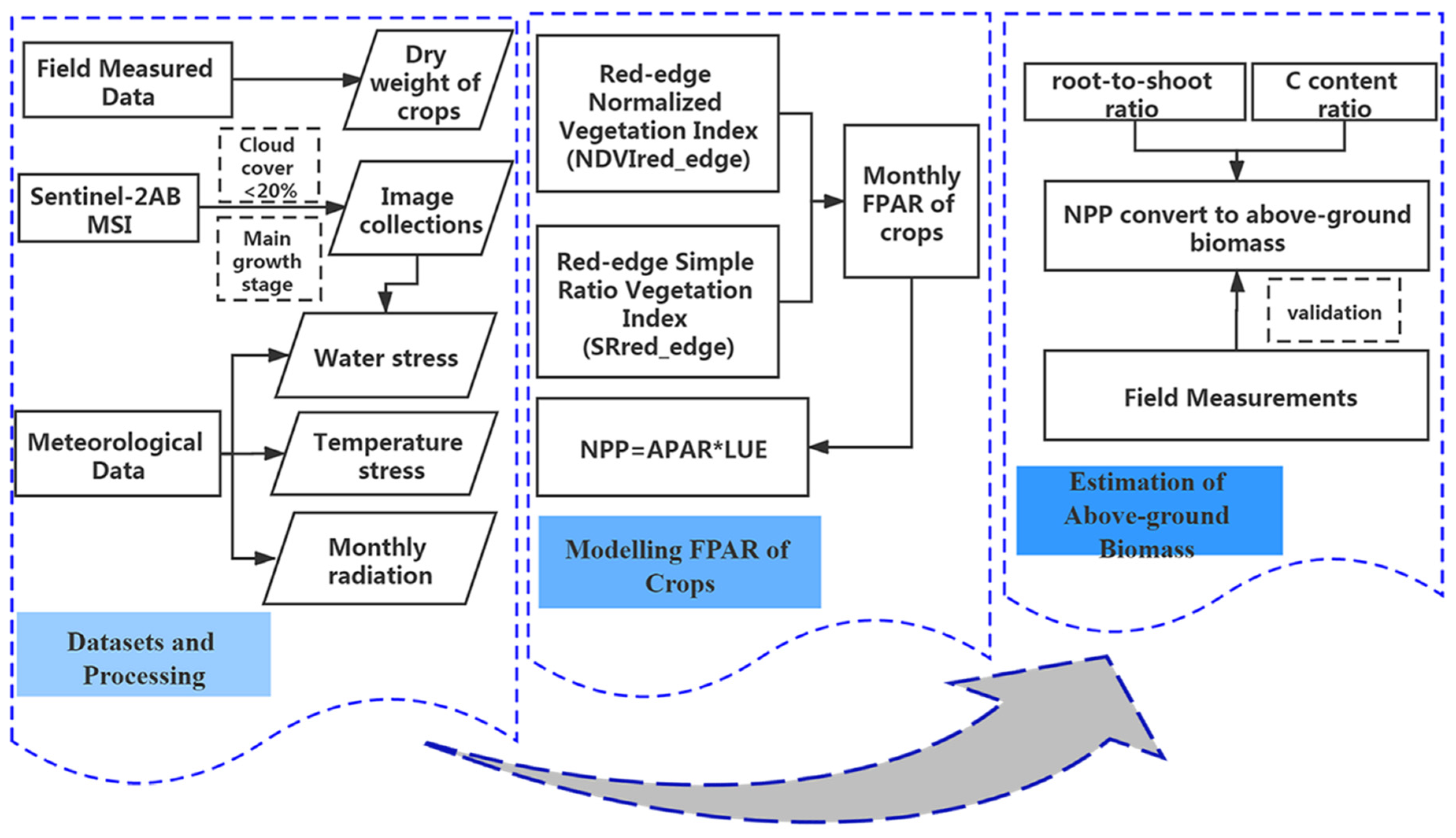
The workflow is shown in Figure 4, and it mainly included the following three parts: datasets and processing, modeling the FPAR of crops, and estimation of aboveground biomass. For the data collection and processing, we collected the measured data, Sentinel-2 multispectral data, and meteorological data. We processed the Sentinel-2 image collections of the two main crops growing seasons, including the cloud threshold setting, image clipping, and other preprocessing steps. The meteorological data mainly included the monthly precipitation, temperature, and sunshine hours, which were used to calculate the temperature stress and solar radiation. For the crop FPAR modeling, we modeled the FPAR based on NDVIred-edge, SRred-edge from previous research and the experiments in this study. For the estimation of aboveground biomass, we gathered all of the input parameters of the improved CASA model, and then input them into the model to obtain the estimated crop biomass. According to the root-to-shoot ratio and the ratio of carbon content, the NPP was transformed into the aboveground biomass, and the aboveground dry weight data of winter wheat and summer maize were used to validate the accuracy of the biomass estimated by the improved CASA model.
3. Results
3.1. Modeling of FPAR Based on Red-Edge Vegetation Indices
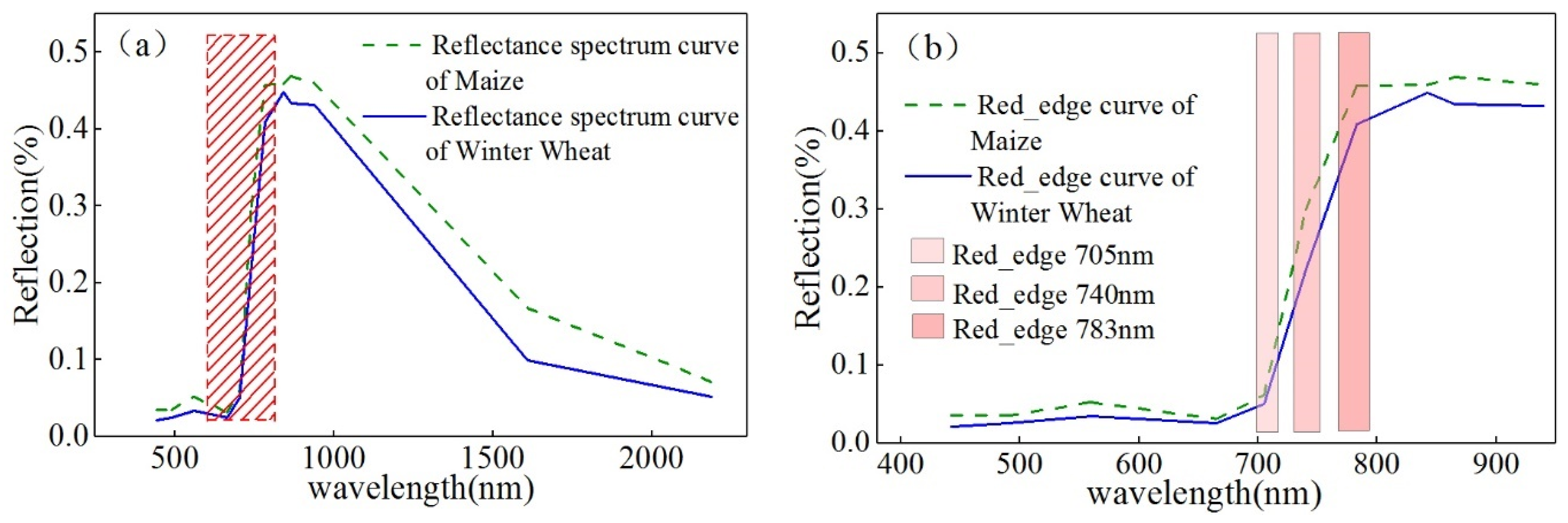
To explore the potential of the inversion FPAR with red-edge information, we first analyzed the variation characteristics of winter wheat and summer maize in the red-edge spectral range of Sentinel-2 data. In order to reduce the influence of other factors (cloud, spectral noise, etc.) on crop spectral variation in the growing season, we selected the seasonal average spectral curves of winter wheat and summer maize in the same sample point of two crops in different growing seasons, and drew the variation curves of canopy spectral reflectance of two crops from blue to short-wave infrared band (see Figure 5).
Figure 5a shows the variations in the spectral reflectance curves and red-edge information in the main growing seasons of the two crops. In Figure 5b, the rate of changes in summer maize within 705 nm of the red-edge is higher than that of winter wheat, because the photosynthetic efficiency of summer maize (C4 crops) is usually higher than that of winter wheat (C3 crops) [49]. However, the change rates of winter wheat and summer maize in the range of 740 and 783 nm of the red edge are basically the same, which indicates that in this interval, the red-edge spectrum is insensitive to the chlorophyll of the two crops. Previous research has also shown that the positions of the crops at a red-edge of 705 nm are more suitable for the inversion of the bio-physiological parameters [17,50].
Therefore, we used the red-edge vegetation indices and to fit the MCD15A3H LAI/FPAR products in the corresponding crop growing season, and the inversion results are shown in the following figures.
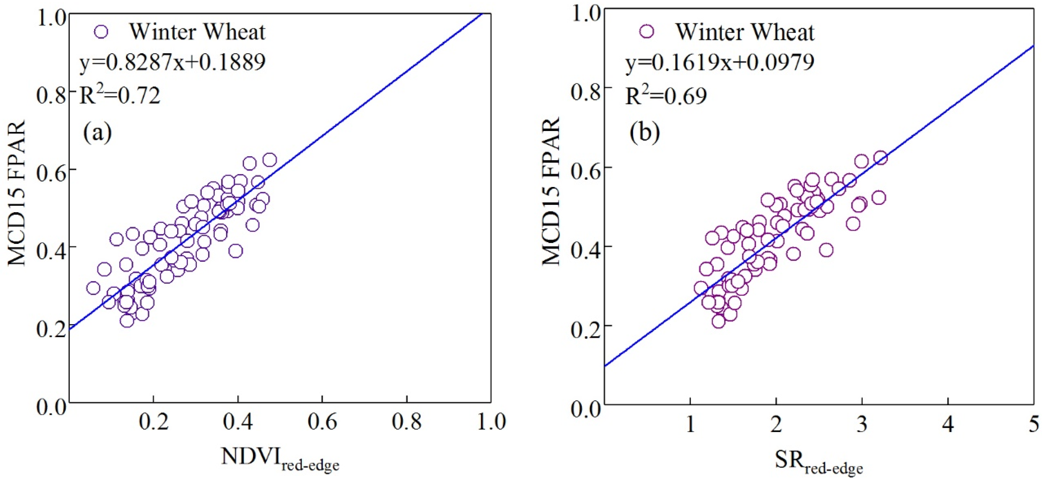
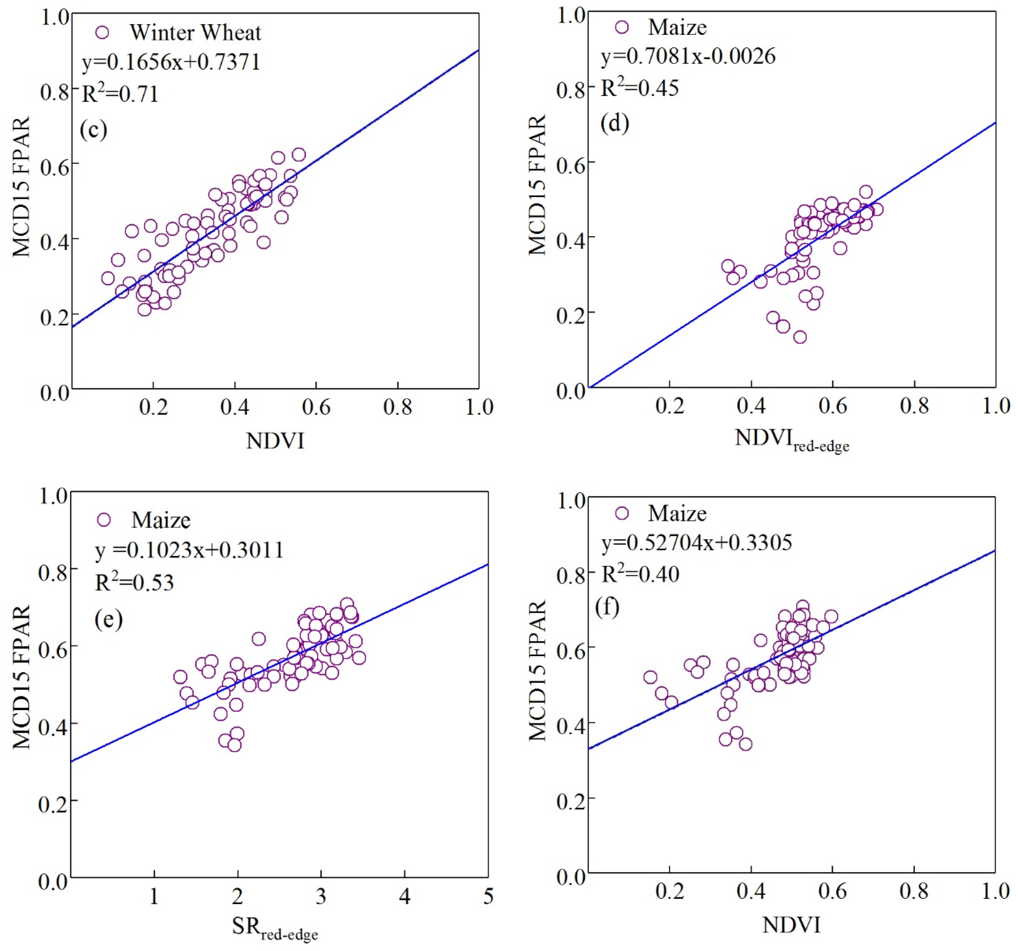
Figure 6 shows the regression accuracy of the NDVI-related vegetation indices in the main growing seasons of winter wheat and summer maize. The results show that the fitting accuracy of the and with the MODIS FPAR data is higher than that of the original model, NDVI. This indicated that the and are more sensitive to the detection of the vegetation’s photosynthetically active radiation and that they have better retrieval performance.
The table above lists the fitting models and accuracies of , , and NDVI in the main growing seasons of the two crops. The fitting accuracies of the , , and NDVI during the winter wheat growing season are 0.72, 0.71, and 0.64, respectively (Table 4). has the highest fitting accuracy, which is higher than those of and NDVI by 0.01 and 0.03. In the maize growing season in the summer, the fitting accuracies of the , and NDVI are 0.45, 0.53, and 0.40, respectively. has the highest fitting accuracy of 0.53, which is higher those of the and NDVI, which have fitting accuracies of 0.08 and 0.13. The original model’s NDVI has the lowest fitting accuracy. Therefore, this study models the inversion formula for improving key parameter, FPAR, for different crop types.
where and refer to the FPAR values of winter wheat and maize. and refer to the red-edge vegetation indices of winter wheat and maize. In order to reduce the influence of extreme values, 95% and 5% confidence intervals are used for the maximum and minimum values, respectively. Equations (15) and (16), proposed in this study, comprise the most fundamental difference between the improved CASA and the original CASA model for the FPAR inversion method. Considering the sensitivity of the narrow-band red-edge vegetation index in retrieving the crop LAI, chlorophyll content, biomass, and other biophysical parameters, the red-edge vegetation indices are used to retrieve the FPAR. For this study, in the main growing seasons of winter wheat and summer maize, the accuracy of the FPAR retrieved by is higher, while is more accurate in retrieving the FPAR of maize.
3.2. FPAR Inversion Results Based on Red-Edge Vegetation Indices
According to Equations (8) and (9), this research used the red-edge vegetation indices to retrieve the FPAR of crops (Figure 7 and Figure 8). The maximum value of the FPAR in the main growing season of winter wheat appeared in May, and the maximum value was 0.91. The maximum value of the FPAR in the main growing season of summer maize was in August, and it was 0.91. Accordingly, the vegetation index of the two crops also reached the maximum in May and August, respectively.
In March, after the greening stage of winter wheat, the stalks and leaves of the winter wheat grew at the jointing stage, and the ability of the leaves to absorb solar radiation was gradually strengthened. In April, the winter wheat entered the booting stage after the jointing stage, the further growth of the leaves basically reached a normal level, and the ability of the canopy to absorb solar radiation was significantly improved. In May, the winter wheat leaves basically expanded to the largest area, and most plants were in the flowering period. Moreover, the NDVIred-edge and FPAR also reached the maximum.
In July, the summer maize entered the jointing stage after the seedling stage, three-leaf stage, and seven-leaf stage, and the height of the leaves and plants increased. In August, the summer maize entered the flowering and tasseling period, the leaves were basically developed, and the ability to absorb solar radiation was further improved. In September, the summer maize gradually shifted from the vegetative growth stage to the reproductive growth stage. After the silking and maturity stages, the grain filling was basically completed, and the thousand-grain weight increased significantly. At this time, the ability of the leaves to absorb photosynthetically active radiation was reduced, which, in turn, led to a decrease in the FPAR value.
3.3. Improved Inversion Results Based on Red-Edge Vegetation Indices
3.3.1. Cumulative NPP and Biomass of Crops
In the above research, the improved CASA was used to model the FPAR in the main growing seasons of the crops. It can be seen in Equation (5) that there was a significant linear relationship between the aboveground biomass and accumulated NPP. When the plant root-shoot ratio and C content parameters were determined, the NPP could be transformed into the plant aboveground biomass. Winter wheat and summer maize have different primary products that assimilate carbon dioxide in photosynthesis, and they are divided into C3 and C4 plants. Therefore, the carbon content of the plants is also different. At the same time, due to differences in crop types and growth characteristics, there are also differences in the root-shoot ratios of winter wheat and summer maize (Table 5). These factors must be considered when converting the NPP into biomass.
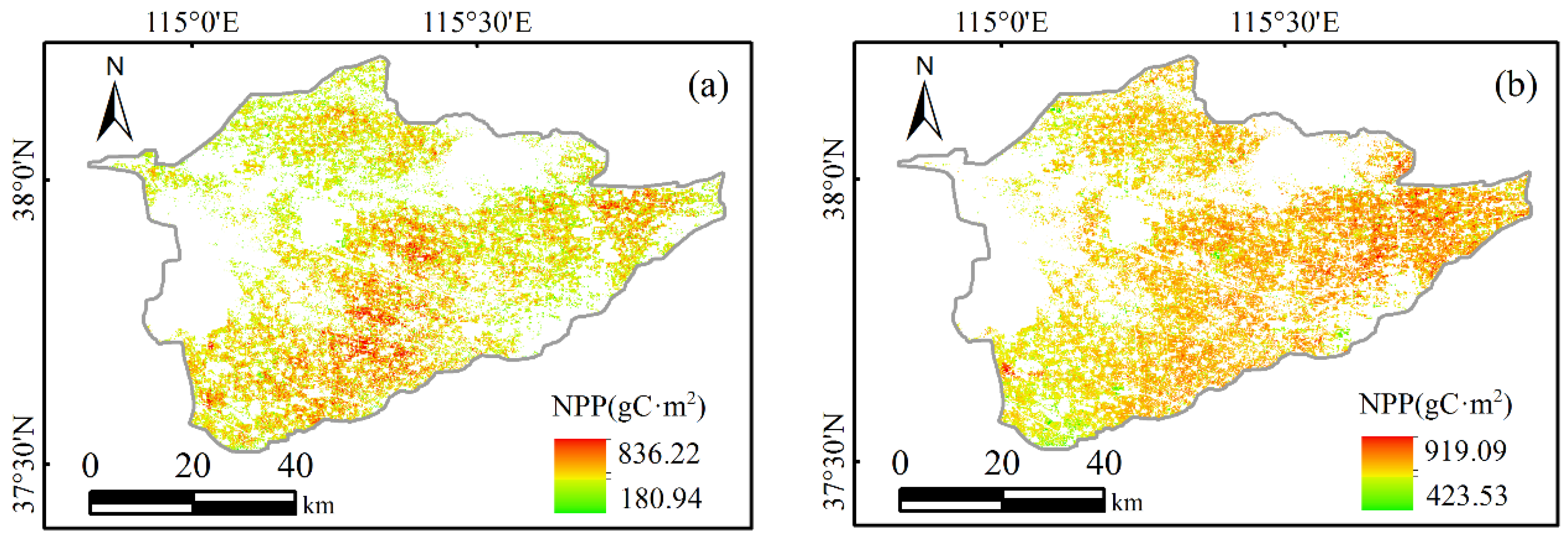
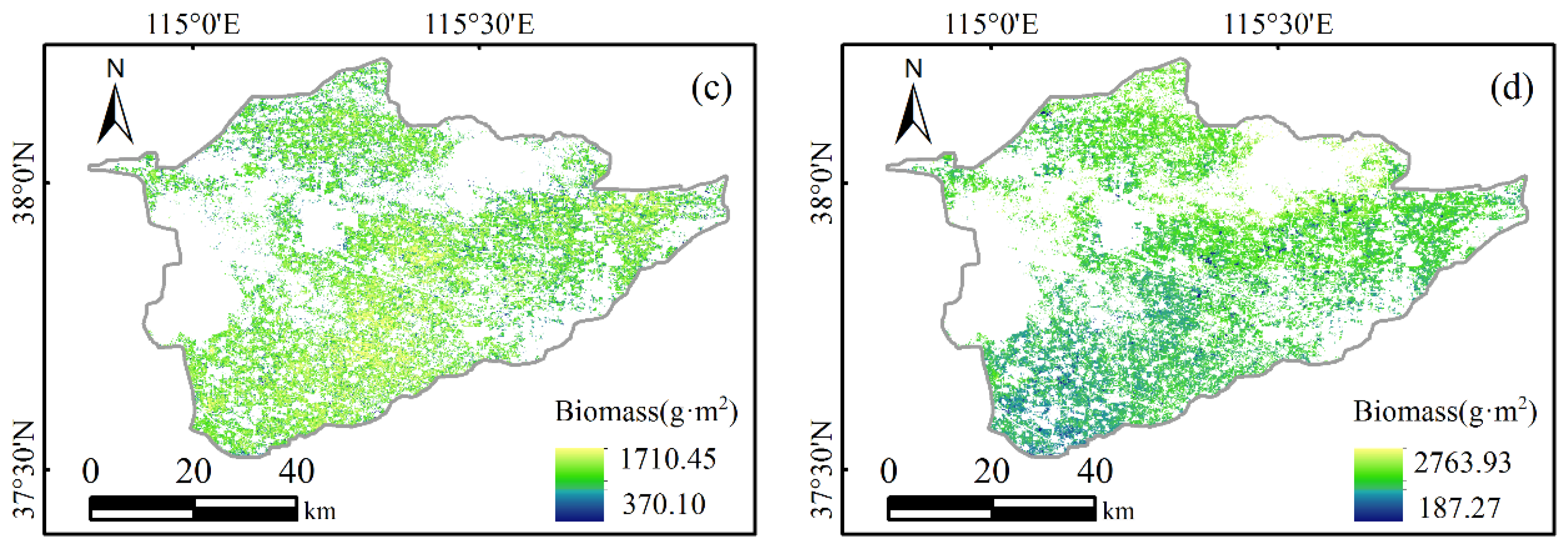
When the carbon content and root–shoot ratio parameters of winter wheat and summer maize were determined (Table 5), the cumulative NPP could be converted into the aboveground biomass of the crops with Equation (12) (see Figure 9a,b). Figure 9c,d illustrates the spatial distribution map of the aboveground biomass of winter wheat and summer corn in the Shijin irrigation area of Hebei Province in 2019. According to the map, we found that there were differences in the biomass changes and spatial distributions of winter wheat and summer corn in the study area. The biomass of winter wheat varied from 487.67 to 1585.08 g·m−2. From the perspective of spatial distribution, the biomass in the southeastern part of the study area was the largest, while the biomass in the northwest was relatively small. The biomass of summer maize varied from 187.27 to 2763.93 g·m−2. The maximum biomass value was mainly distributed in the northwest, and the minimum value was mostly distributed in the south. Due to the linear relationship between the NPP of winter wheat and summer maize and the biomass, regardless of the influence of other factors, the spatial distribution of the biomass was similar to the spatial distribution of the accumulated NPP.
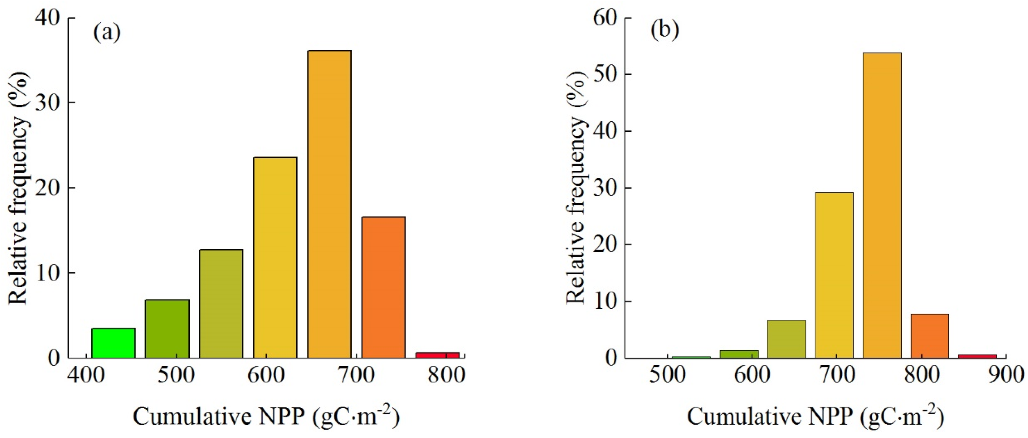
According to the cumulative NPP frequency distribution maps of the two crops, the cumulative NPP of winter wheat was mainly concentrated in the 600–700 gC·m−2 interval. The cumulative frequency of the NPP reached the maximum value of 670 gC·m−2, and the relative distribution frequency was close to 40% (Figure 10a). For the cumulative NPP distribution frequency map of maize, the cumulative NPP was mainly concentrated in the 700–800 gC·m−2 interval, the NPP cumulative frequency reached the maximum value of 753 gC·m−2, and the relative distribution frequency was close to 60% (Figure 10b).
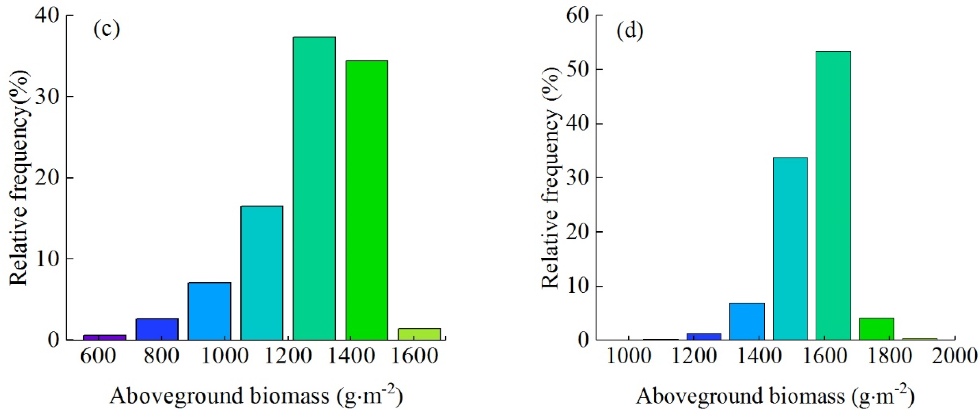
Moreover, in order to analyze the distribution of the aboveground biomass of winter wheat and summer maize, the relative frequency maps of their distributions in different intervals were calculated (see Figure 10c,d). For the distribution frequency map of the aboveground biomass of winter wheat, the biomass was mainly concentrated in the range of 1000–1500, and the maximum biomass frequency was 1284 g·m−2, with a relative distribution frequency of more than 30%. For the distribution frequency map of summer maize’s cumulative biomass, the cumulative NPP was mainly concentrated in the range of 1200–1800. The maximum biomass cumulative frequency was 1627 g·m−2, and the relative distribution frequency was close to 50%. As such, the cumulative biomass distribution of winter wheat and summer maize was close to the standard normal distribution, but their concentration frequency distribution intervals were different, which indicated that the average biomass of summer maize was higher than that of winter wheat.
3.3.2. Aboveground Biomass Estimation Accuracy of Crops
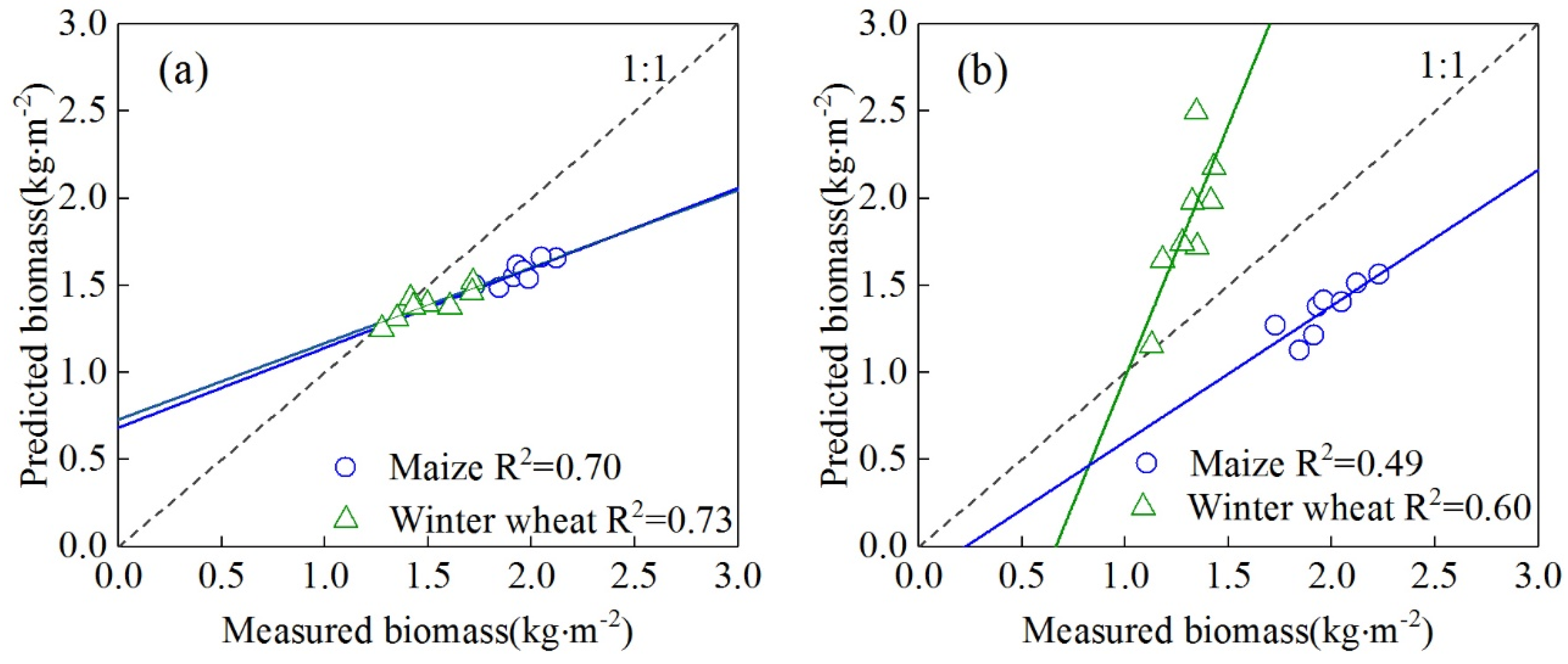
The correlation between the aboveground biomass data of winter wheat and summer maize and the predicted aboveground biomass was analyzed (see Figure 11).
According to the correlation analysis of the prediction results of the two models, we found that the aboveground biomass data predicted by the improved CASA model have an obvious linear correlation with the measured aboveground biomass data. Figure 11a shows the relationship between the predicted biomass of the model and the measured biomass of winter wheat. The result indicates that there is a significant linear relationship between them, R2 is 0.73. For the predicted and measured biomass of summer maize, the R2 is 0.70, and the linear relationship was significant. However, the accuracy of the predicted biomass of the original CASA model is lower than the improved CASA model (Figure 11b). The accuracies of predicted biomass of winter wheat and summer maize are 0.6 and 0.49, respectively, which are lower than those of the improved CASA model.
As such, according to the linear relationship between the predicted value and the measured value of the improved CASA model, the correlation between the predicted value and the measured data is significant, which can effectively estimate crops’ biomass in the study area.
3.4. Seasonal Variation and Factors Influencing Crops Aboveground Biomass
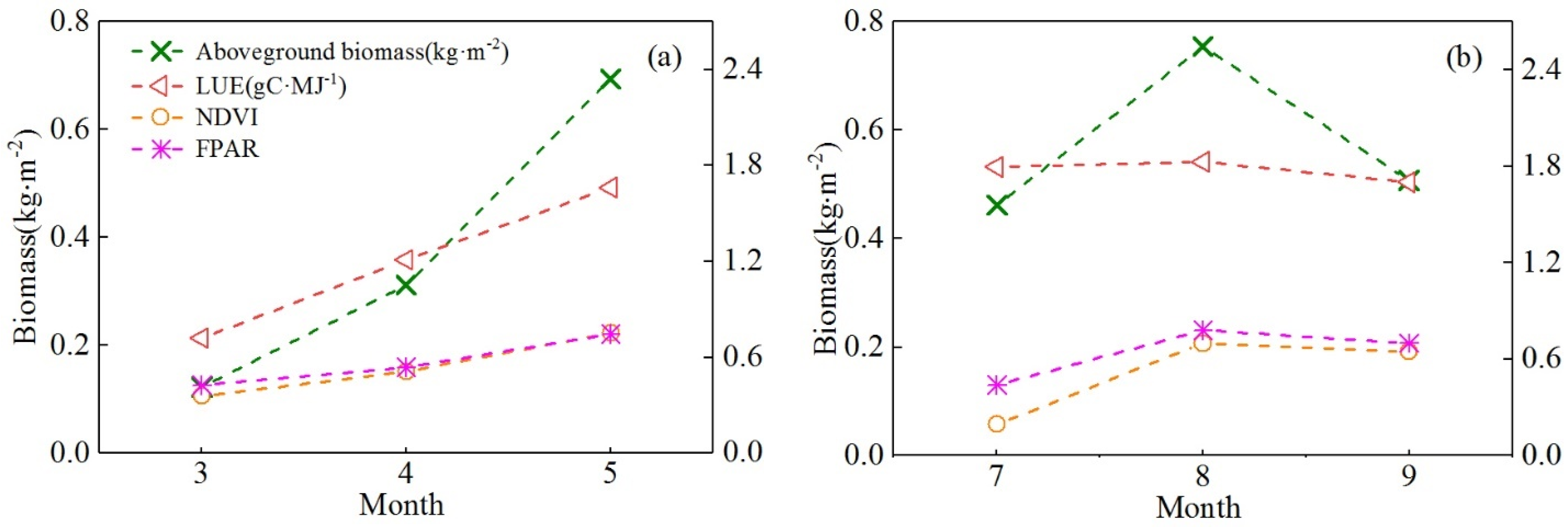
To further explore the seasonal changes in the NDVI, FPAR, LUE, and biomass in the key growing seasons of winter wheat and summer maize and to understand their inherent growth rules, we analyzed the variations in the NDVI, FPAR, LUE, and biomass in different months of the main growing seasons of winter wheat and summer maize (Figure 12), as well as the effects of the NDVI, FPAR, and LUE on the crops’ biomass.
In the main growing season of winter wheat (March to May), the NDVI value showed a significant increasing trend, which reached the maximum value in May (Figure 12). At this stage, the stems, leaves, and other tissues of winter wheat grew and developed completely. The ability to absorb solar radiation and the photosynthesis of leaves reached the maximum. For summer maize, the NDVI increased first, and then slowly decreased, but the overall trend was increasing. In September, summer maize turned from vegetative growth to reproductive growth, and entered the milk stage and early mature stage. The photosynthetic function of the leaves decreased and the NDVI gradually decreased. The monthly average FPAR values of the winter wheat and summer maize varied in the main growing seasons but showed an increasing trend. Moreover, the trend of the FPAR was consistent with the NDVI.
The LUE of the two crops also changed dramatically in the main growing season. From March to May, the LUE value of winter wheat increased linearly from low to high, and it was consistent with the change trend of the NDVI and FPAR parameters. In the main growing season of summer maize, although the LUE value in August was slightly higher than that in July, the LUE value decreased again in September, which led to the overall downward trend in the final growing season. This is because in the main growing season of wheat, the environmental stress factors gradually decreased and the LUE increased. However, in the late growth stage of summer maize, it was greatly affected by temperature and precipitation stress, and the LUE gradually decreased. For winter wheat, the seasonal biomass showed an increasing trend. The minimum biomass value was at the jointing stage of winter wheat, and then it began to rise. In May, the biomass of winter wheat reached the maximum. At this stage, the flowering stage of winter wheat gradually ended, and it later entered the milky stage. This indicated that winter wheat changed from the vegetative growth stage to the reproductive growth stage. The seasonal biomass of summer maize showed a slight upward trend. In August, all tissues and organs of summer maize developed completely. Summer maize grew until September and reached the late stage of reproductive growth. The stems, leaves, and other organs of maize began to wilt, the grain filling of maize ended, and the 1000-grain weight reached the maximum.
The biophysical parameters NDVI, FPAR, and biomass of the two crops have an obvious increasing trend in the main growing seasons, except for slight differences in LUE values. In the growing season of winter wheat, the parameters NDVI, FPAR, and LUE increased gradually due to the reduced stress from environmental factors, which promoted the growth of biomass. In the late growth stage of summer maize, with the aggravation of water and temperature stress, the NDVI, FPAR, and LUE showed a downward trend, which affected the biomass accumulation.
4. Discussion
4.1. Accuracy Differences of Various Vegetation Indices
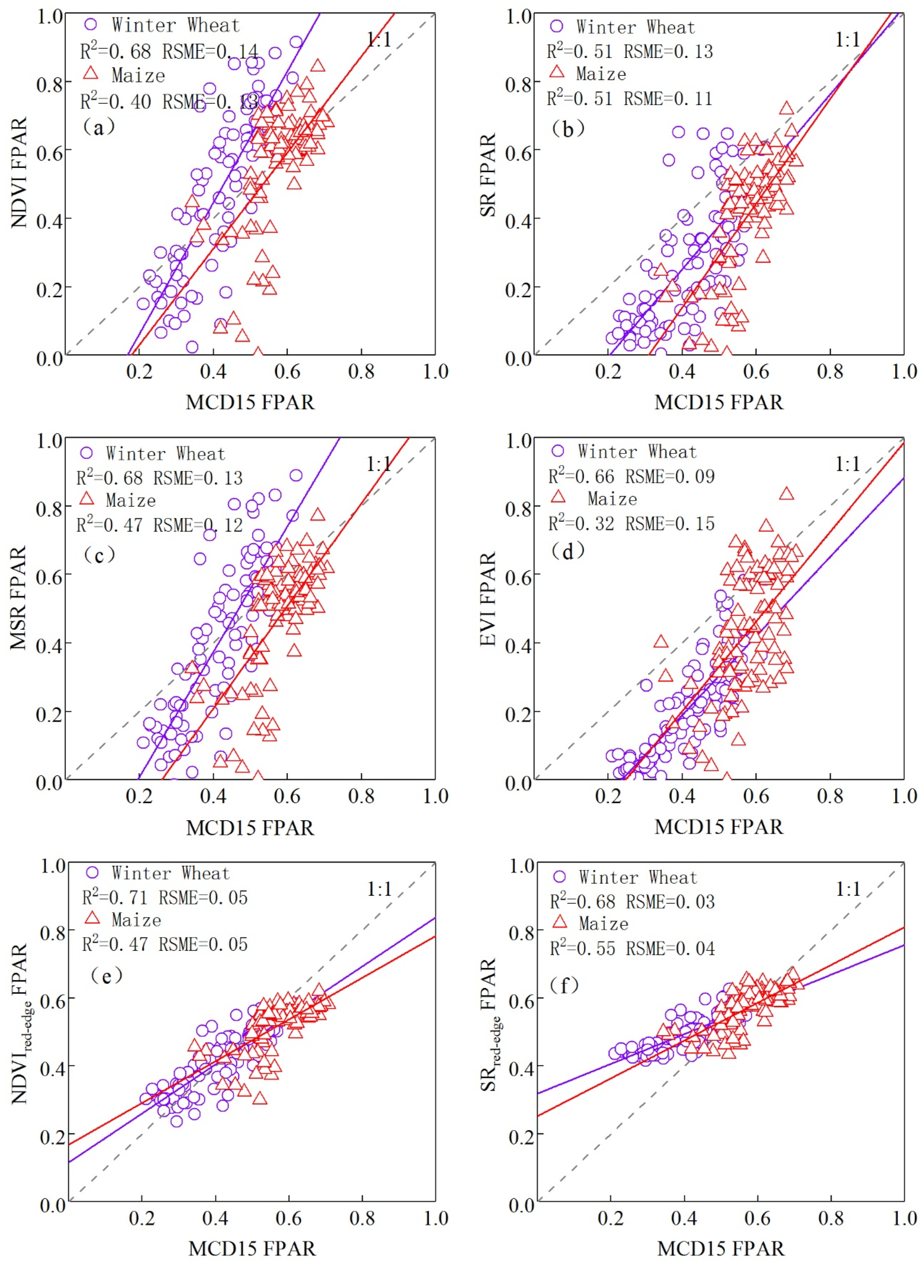
The FPAR is one of the two most important input parameters of the CASA model, and the accuracy of its inversion directly affects the output of the model. Compared with previous studies and experimental results, it was found that the inversion accuracy of the FPAR based on the and was higher than that of the NDVI in the original model, but the inversion effects of other vegetation indices were not compared. Therefore, in order to discuss the uncertainty of FPAR inversion in the CASA model, this study analyzes the inversion effects of other vegetation indices. Many studies have shown that there is a significant correlation between crop FPAR and certain vegetation indices, and these vegetation indices are used to invert the FPAR. Kumar, Seller et al. found a linear relationship between the FPAR and SR through theoretical research. Potter et al. began to use the SR to estimate the FPAR with the CASA model. Hatfield et al. [40] found that the FPAR and NDVI of wheat and other crops also had a strong linear relationship. Recently, some scholars found that combining the SR and NDVI to invert the FPAR value is the most accurate. All of these indicate that the crop FAPR has different correlations with vegetation indices.
In improved CASA model, the FPAR values were estimated based on its relationship with the and . Moreover, to explore the inversion differences of FPAR with different vegetation indices, we analyzed the inversions accuracies of FPAR of the red-edge indices and non-red-edge indices including NDVI, SR, NDVI-SR, MSR, EVI, , and.
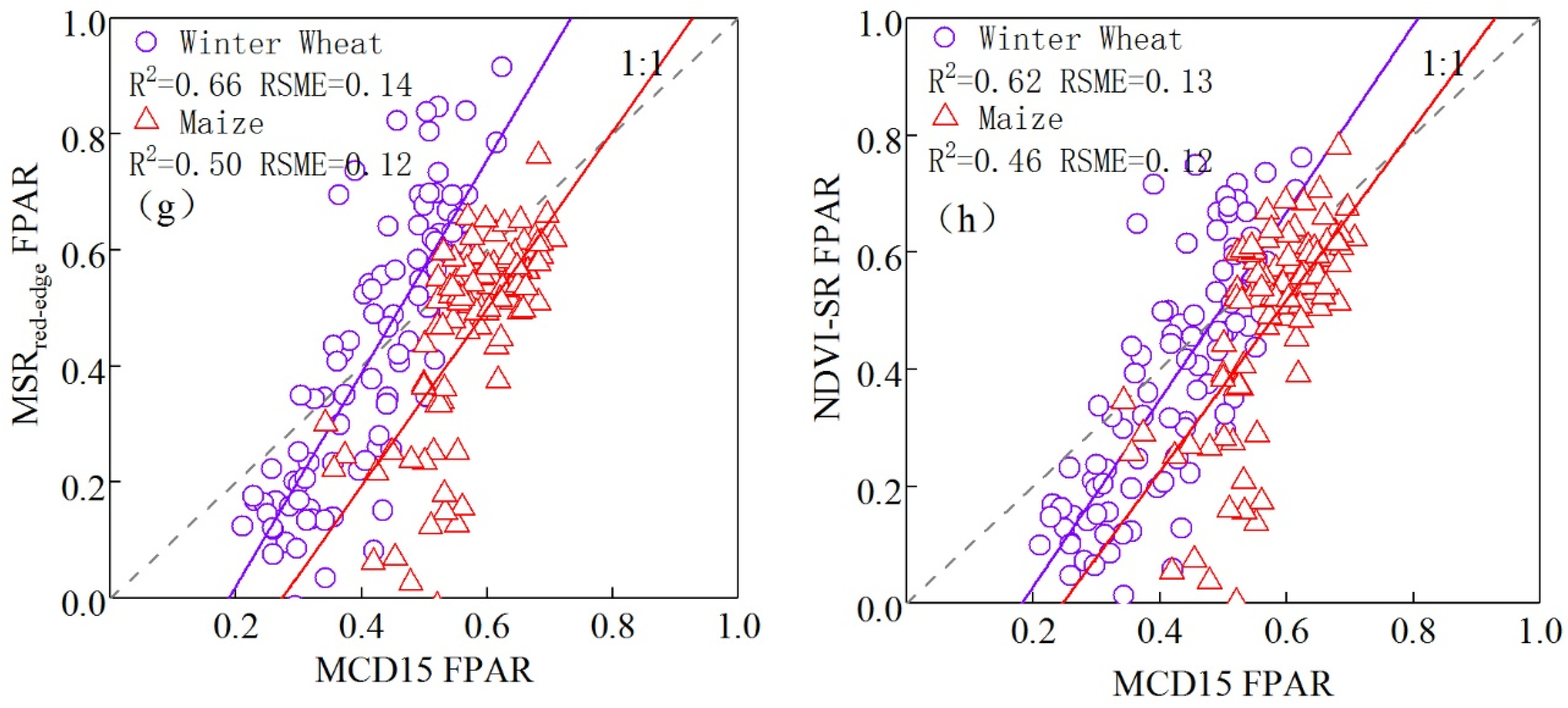
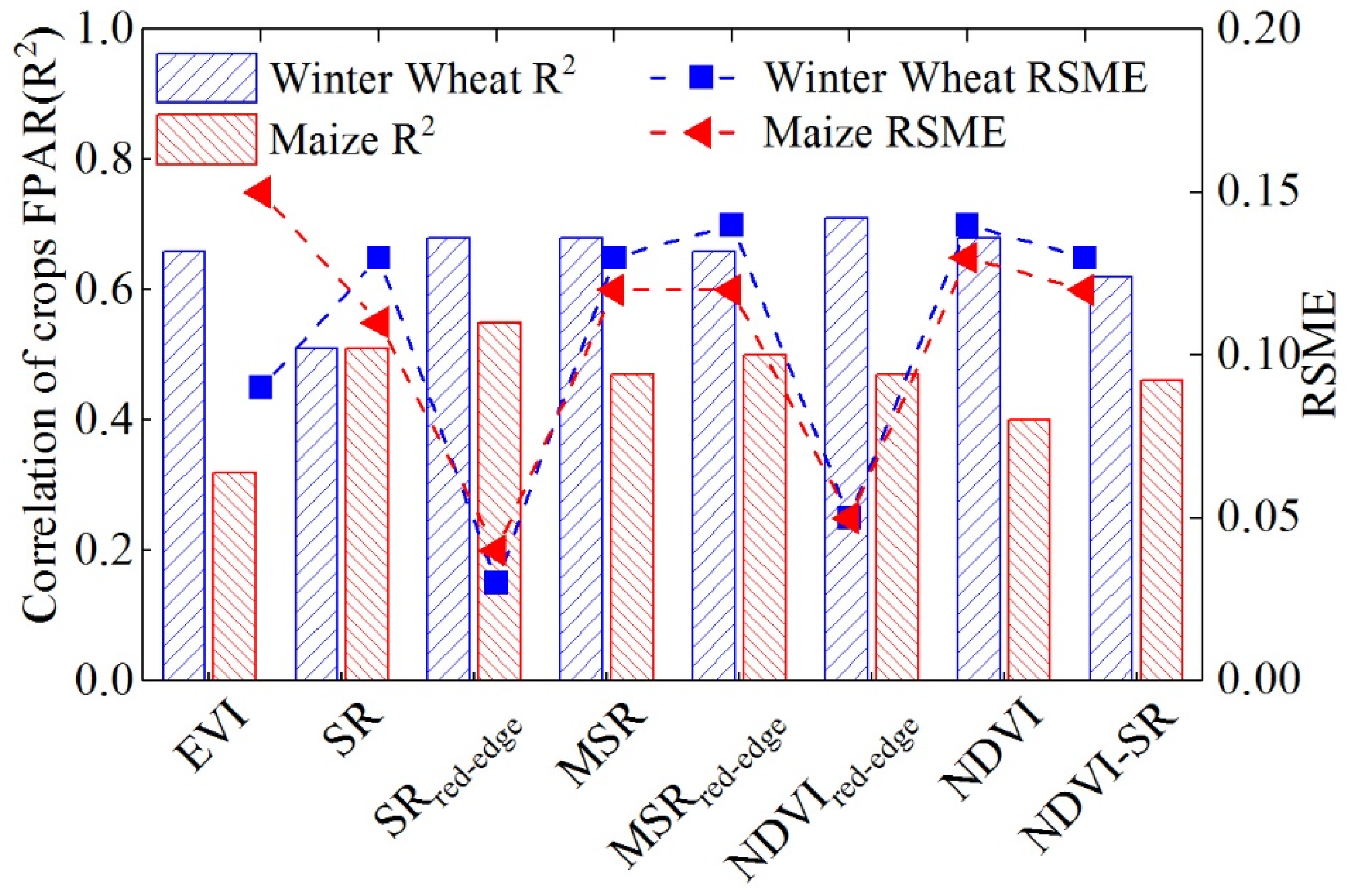
According to the FPAR accuracy of the NDVI-SR inversion in the original CASA model and the FPAR correlation analysis results of the inversions of the above seven vegetation indices (Figure 13 and Figure 14), the FPAR accuracies of the red edge and red-edge inversion in this study were both higher than those of the other vegetation indices. The winter wheat FPAR retrieved with the was the largest, with an R2 of 0.71 and RSME of 0.05. The accuracy was higher than that of the winter wheat FPAR retrieved with the NDVI-SR. For inversion with , the maximum FPAR accuracy of summer corn was 0.55, and the RSME was 0.04. The retrieval accuracy was higher than that of the summer corn FPAR retrieved with the NDVI. This also shows that the red-edge information of Sentinel-2 helps to improve the accuracy of the FPAR inversion.
4.2. Mapping Differences of Various Models
The FPAR and NPP are important for monitoring the growth and development of vegetation, and they provide a good indication of the productivity of terrestrial ecosystems. The improved CASA model based on the red-edge vegetation index proposed in this study showed better performance in the FPAR inversions of winter wheat and summer maize and in the estimation of aboveground biomass; it was also more indicative of the crop production capacity. Previous studies assumed that the FPAR of vegetation would be affected by the attributes of the leaf photochemical elements (such as chlorophyll, etc.), spatial distribution, and canopy structure (LAI and leaf angle), such as the NDVI, SR, etc. [37,51]. Based on the multispectral data, we found that crops’ FPAR also had a stronger relationship with the combination of the red and red edge bands. Moreover, when the red-edge vegetation indexes, red and red1, were fitted to the MODIS FPAR products, the fitting accuracy was higher than the accuracy of the wide-band NDVI inversion in the original model. Moreover, the red-edge vegetation indices and were used to fit the MODIS FPAR products, and their fitting accuracies were higher than that of the wideband NDVI in the original model. This shows that, compared with the wide-band vegetation NDVI (near infrared: 800 nm) in the original CASA model, the red-edge vegetation index (red edge: 705 nm) was more sensitive to the detection of crops’ photosynthetic levels. Similarly, for the estimated aboveground biomass of crops, the accuracy of the aboveground biomass of winter wheat and summer maize estimated by the improved CASA model was higher than that estimated by the original CASA model. This is because the improved CASA model is based on the red-edge vegetation indices. If other variables remain unchanged, the higher the accuracy of the FPAR retrieved by the red-edge vegetation indices, the higher the accuracy of the final aboveground biomass estimation. To further analyze the mapping details of the CASA model, the original CASA model, and MODIS FPAR product, we randomly selected a sub-region in the study for discussion.
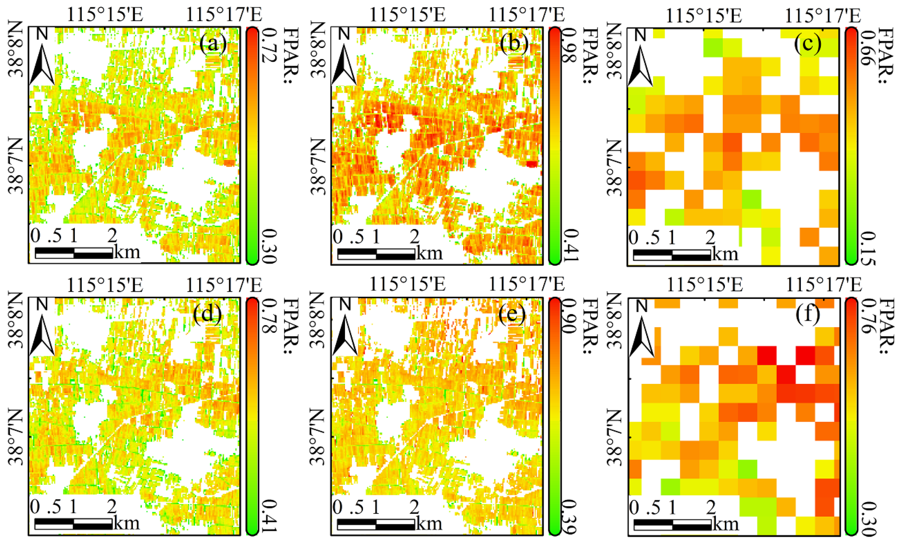
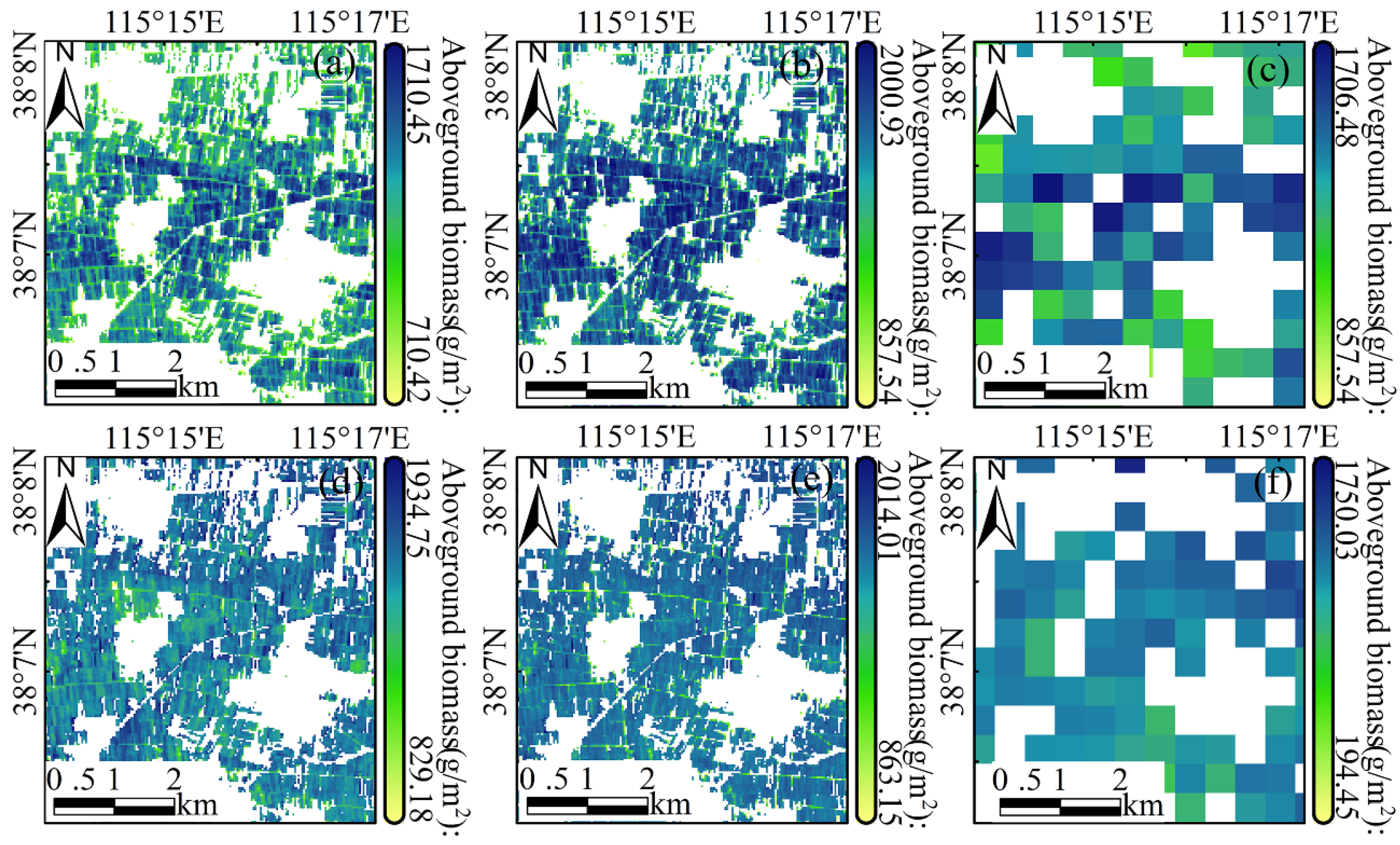
Compared with the FPAR and MODIS FPAR product retrieved by NDVI, the red-edge vegetation indices have a higher accuracy for FPAR mapping in sub-regions. Moreover, those results have better consistency with the MODIS FPAR product (Figure 15). For the two crops FPAR retrieved by NDVIred-edge and SRred-edge, we find that the 10 m FPAR mapping based on the red-edge vegetation indices is in good agreement with the MODIS FPAR product in spatial distribution and numerical range (Figure 15a,d). The value of FPAR retrieved by NDVI is higher than FPAR retrieved by red-edge indices and MODIS FPAR. This is because the NDVI value of the combination of near-infrared and red band is larger, and it is close to saturation in dense vegetation. Moreover, Figure 14 shows the spatial distribution of aboveground biomass based on improved CASA model, the original CASA model and the MODIS FPAR-driven. The result shows that the aboveground biomass of 10 m predicted by the improved CASA model and driven by MODIS FPAR are also in accordance with spatial distribution and numerical range (Figure 16a,d). The original CASA model based on NDVI, despite the spatial distribution consistent with the aboveground biomass of improved CASA model and MODIS FPAR-driven, shows a significant overestimation of its biomass (Figure 16b,e).
The above analysis indicates that the FPAR and biomass mapping of crops with high spatial resolution based on red-edge vegetation indices are more helpful for quantitative analysis of crop growth and change than those with coarse resolution. According to previous studies, the CASA model based on the wide-band vegetation NDVI is effective in estimating ecosystem productivity, carbon fixation, biomass, etc. [22]. The red-edge band has been proven to have an obvious relationship with some biophysical parameters of plants. Using the red-edge band to construct red-edge vegetation indices can help improve the estimation accuracy of vegetation chlorophyll content, biomass, and productivity [52,53]. For global and national scales vegetation biomass estimation, the improved CASA model based on the red-edge vegetation index still has great application potential.
4.3. Features of Improved CASA Model
The improved CASA model is applied to our work and the better estimation results are obtained. Specifically, we believe that there are several factors that can improve the accuracy of the improved CASA model in estimating crop biomass.
The FPAR model based on red-edge vegetation indices can better reflect the inversion of crops FPAR. Since Potter first applied CASA to the study of global vegetation NPP and carbon change model, more researchers introduced the CASA model to global or regional vegetation, crop NPP, biomass and carbon change, which undoubtedly promoted the application of the CASA model. However, limited to satellite sensors, many researchers can only use the existing satellite images. For example, Potter and Rummy used NOAA AVHHR data to analyze the change of global NPP. The satellite data has only four channels, namely red light (R: 0.58–0.68 μm), near infrared (NIR: 0.73–1.1 μm), thermal infrared 1 (10.2–11.3 μm) and thermal infrared 2 (11.5–12.5 μm). Although the NDVI based on the combination of red and near-infrared channels can roughly reflect the growth status of vegetation, the CASA model based on AVHHR cannot accurately monitor the change of vegetation NPP due to the influence of spatial resolution and spectral resolution of sensors. With the development of satellite sensors, such as MODIS, Landsat, Rapid Eye and Sentinel-2, the higher the spatial resolution, the more detailed the spatial distribution of vegetation.
In addition, the enhancement of spectral resolution is an important reason for the improvement of quantitative remote sensing inversion accuracy. The difference of different vegetation types and the capacity of photosynthesis directly affect the spectral changes. The quantitative analysis of different spectra can more effectively reflect the growth mechanism of crops. Various sensitive vegetation indices can also accurately retrieve crop physiological parameters. In this study, combined with previous studies and intensive experiments, we found that compared with the original CASA model of NDVI based FPAR, NDVIred-edge and SRred-edge can retrieve crops FPAR more effectively. This is due to the faster change of canopy reflectance at 705 nm of red edge, which leads to more sharp response to crops chlorophyll. Compared with the former two, the canopy reflectance at 842 nm of NDVI does not change dramatically, so the accuracy of FPAR inversion is lower than that of red edge based FPAR, which leads to the low accuracy of biomass estimation.
The main feature of our work is to propose a red edge based FPAR model based on sentinel-2msi data. The model is quickly fitted by MODIS FPAR products with higher accuracy, and then input into CASA model. However, there are differences in spatial resolution and radiation resolution between MODIS FPAR and sentinel-2, which affect the accuracy of FPAR and biomass estimation to a certain extent. Some research found that MODIS FPAR (C6) is considerably better than C5 with lower RSME [54,55]. Although both C5 and C6 products overestimate the FPAR in sparse vegetation areas, the impact on dense crop areas is relatively small. Overall, MODIS FPAR can accurately reflect the photosynthetic capacity and other physiological parameters of crops in the main growing season. In the absence of measured FPAR data, it is a practical method to use the fitting model of vegetation index and MODIS FPAR to inverse FPAR.
5. Conclusions
Aboveground biomass mapping is crucial for agricultural production management and food security, and the CASA model provides important support for this purpose. The following conclusions can be drawn:
First, the accuracy of the FPAR retrieved by the and is higher than that of the wide-band vegetation NDVI. The NDVI tends to saturate in dense vegetation, which affects the estimation of the FPAR and biomass. This research used , that is more sensitive to vegetation changes to fit the MODIS FPAR product. The results show that the FPAR inversion accuracies of the red edge were 13% and 20% higher than that of the original CASA model.
Second, obviously seasonal differences of the NDVI, FPAR, and LUE of different crops are reflected in our work. The variations of biophysical parameters of crops shows that, due to the effects of decreased temperature and precipitation stress, four biophysical parameters all display an increasing trend. The maximum values of the parameters all appeared in May, with a progressive increase trend. However, four biophysical parameters during the main growth of summer maize, showed shock downward trend at an aggregate level. The maximum of the four parameters appeared in August, indicating that the temperature and precipitation stress of the crops was the lowest at this stage, which affect the aboveground biomass accumulation of crops.
Overall, an improved CASA model was utilized to estimate aboveground biomass of crops and achieved a good performance. In future research, the development of UAV and high-revolution, real-time FPAR, biomass products will help to improve the potential accuracy of the CASA model.
Author Contributions
Conceptualization, P.F., N.Y. and X.Z.; methodology, P.F., N.Y. and X.Z.; writing—original draft preparation, P.F., P.W. and Y.Z.; writing—review and editing, X.Z. and N.Y.; supervision, X.Z. and N.Y. All authors have read and agreed to the published version of the manuscript.
Funding
This research was funded by the Strategic Priority Research Program of the Chinese Academy of Sciences (Grant No. XDA19030202), the National Key Research and Development Program of China (2018YFE0107000), the National Key Research and Development Program of China (2021YFE0106700), the Key Technologies R&D Program of Henan Province (212102110033), Global Environment Facility (GEF), the integrated management mainstreaming project of water resources and water environment (MWR-C-3-9), and the Qinghai Science and Technology Plan (Grant No. 2019-SF-155).
Institutional Review Board Statement
Not applicable.
Informed Consent Statement
Not applicable.
Data Availability Statement
Sentinel-2 data and MCD15A3H data are openly available via the Google Earth Engine, and other data are available upon request from the first author.
Acknowledgments
We thank providers of the data for this research: the meteorological data were provided by the China Meteorological Data Service Center (CMDSC). The Sentinel dataset was provided by the European Space Agency (ESA) and Google Earth Engine (GEE) We are grateful to the anonymous reviewers whose constructive suggestions have improved the quality of this study.
Conflicts of Interest
The authors declare that there are no conflict of interest regarding the publication of this paper.
Abbreviations
The following abbreviations are used in this manuscript:
| NPP | Net primary productivity | NPP = APAR × LUE |
| APAR | Photosynthetically active radiation absorbed by the vegetation canopy | APAR = PAR × FPAR |
| FPAR | Photosynthetically active radiation absorption proportion | FPARwheat = 0.8287 × NDVIred-edge + 0.1889 FPARmaize = 0.1023 × SRred-edge + 0.3011 |
| PAR | Photosynthetically active radiation | PAR = SOL × 0.5 |
| SOL | Monthly radiation | Defined as the total radiation of crops in main growth stage |
| LUE | Actual light use efficiency | LUE = Tε1 × Tε2 × Wε × LUEmax |
| LUEmax | Maximum LUE | For winter wheat, LUEmax = 1.95, for summer maize, LUEmax = 2.55 |
| Tε1 | Effects of temperature stress | Tε1 = 0.8 + 0.02 × Topt − 0.0005 × Topt2 |
| Tε2 | Effects of temperature stress | Tε2 = 1.184/{1 + exp [0.2 × (Topt-10-Tx)]} × 1/{1 + exp[0.3 × (−Topt-10 + Tx)]} |
| Topt | Optimal temperature | Defined as the air temperature in the month when the NDVI reaches its maximum |
| Tx | Monthly temperature | Defined as monthly temperature of crops in main growth stage |
| Wε | Effects of water stress | Wε = (1 − (1 + LSWI)/(1 + LSWImax)) + 0.5 |
| LSWI | Land Surface Water Index | LSWI = ()/() |
| B | Aboveground biomass | |
| Ratio of the aboveground biomass to the whole vegetation | For winter wheat, .90, for summer maize, .91, | |
| The C ratio of a crop | For winter wheat, .49, for summer maize, .47, | |
| NDVI | Normalized Difference Vegetation Index | |
| NDVIred-edge | Red-Edge Normalized Difference Vegetation Index | |
| Simple Ratio Vegetation Index | ||
| MSR | Modified Simple Ratio Vegetation Index | |
| MSRred-edge | Modified Red-Edge Simple Ratio Vegetation Index | |
| SRred-edge | Red-Edge Simple Ratio Vegetation Index | |
| EVI | Enhanced Vegetation Index |
References
- Schwalbert, R.A.; Amado, T.J.; Nieto, L.; Varela, S.; Corassa, G.M.; Horbe, T.A.; Rice, C.W.; Peralta, N.R.; Ciampitti, I.A. Forecasting maize yield at field scale based on high-resolution satellite imagery. Biosyst. Eng. 2018, 171, 179–192. [Google Scholar] [CrossRef]
- Li, B.; Xu, X.; Zhang, L.; Han, J.; Bian, C.; Li, G.; Liu, J.; Jin, L. Above-ground biomass estimation and yield prediction in potato by using UAV-based RGB and hyperspectral imaging. ISPRS J. Photogramm. Remote Sens. 2020, 162, 161–172. [Google Scholar] [CrossRef]
- Huang, J.; Ma, H.; Sedano, F.; Lewis, P.; Liang, S.; Wu, Q.; Su, W.; Zhang, X.; Zhu, D. Evaluation of regional estimates of winter wheat yield by assimilating three remotely sensed reflectance datasets into the coupled WOFOST–PROSAIL model. Eur. J. Agron. 2019, 102, 1–13. [Google Scholar] [CrossRef]
- Huang, J.; Sedano, F.; Huang, Y.; Ma, H.; Li, X.; Liang, S.; Tian, L.; Zhang, X.; Fan, J.; Wu, W. Assimilating a synthetic Kalman filter leaf area index series into the WOFOST model to improve regional winter wheat yield estimation. Agric. For. Meteorol. 2016, 216, 188–202. [Google Scholar] [CrossRef]
- Huang, J.; Gómez-Dans, J.L.; Huang, H.; Ma, H.; Wu, Q.; Lewis, P.E.; Liang, S.; Chen, Z.; Xue, J.-H.; Wu, Y. Assimilation of remote sensing into crop growth models: Current status and perspectives. Agric. For. Meteorol. 2019, 276, 107609. [Google Scholar] [CrossRef]
- Fang, P.; Zhang, X.; Wei, P.; Wang, Y.; Zhang, H.; Liu, F.; Zhao, J. The Classification Performance and Mechanism of Machine Learning Algorithms in Winter Wheat Mapping Using Sentinel-2 10 m Resolution Imagery. Appl. Sci.-Basel. 2020, 10, 5075. [Google Scholar] [CrossRef]
- Zhang, X.; Liu, J.; Qin, Z.; Qin, F. Winter wheat identification by integrating spectral and temporal information derived from multi-resolution remote sensing data. J. Integr. Agric. 2019, 18, 2628–2643. [Google Scholar] [CrossRef]
- Zhang, X.; Qiu, F.; Qin, F. Identification and mapping of winter wheat by integrating temporal change information and Kullback–Leibler divergence. Int. J. Appl. Earth Obs. Geoinf. 2019, 76, 26–39. [Google Scholar] [CrossRef]
- Lu, D. The potential and challenge of remote sensing-based biomass estimation. Int. J. Remote Sens. 2006, 27, 1297–1328. [Google Scholar] [CrossRef]
- He, M.; Kimball, J.S.; Maneta, M.P.; Maxwell, B.D.; Moreno, A.; Beguería, S.; Wu, X. Regional crop gross primary productivity and yield estimation using fused landsat-MODIS data. Remote Sens. 2018, 10, 372. [Google Scholar] [CrossRef] [Green Version]
- Goswami, S.; Gamon, J.; Vargas, S.; Tweedie, C. Relationships of NDVI, Biomass, and Leaf Area Index (LAI) for six key plant species in Barrow, Alaska. PeerJ PrePrints. 2015, 3, e913v1. [Google Scholar]
- Sun, Y.; Qin, Q.; Ren, H.; Zhang, T.; Chen, S. Red-edge band vegetation indices for leaf area index estimation from sentinel-2/msi imagery. IEEE Trans. Geosci. Remote Sens. 2019, 58, 826–840. [Google Scholar] [CrossRef]
- Huang, J.; Tian, L.; Liang, S.; Ma, H.; Becker-Reshef, I.; Huang, Y.; Su, W.; Zhang, X.; Zhu, D.; Wu, W. Improving winter wheat yield estimation by assimilation of the leaf area index from Landsat TM and MODIS data into the WOFOST model. Agric. For. Meteorol. 2015, 204, 106–121. [Google Scholar] [CrossRef] [Green Version]
- Huang, J.; Ma, H.; Su, W.; Zhang, X.; Huang, Y.; Fan, J.; Wu, W. Jointly assimilating MODIS LAI and ET products into the SWAP model for winter wheat yield estimation. IEEE J. Sel. Top. Appl. Earth Obs. Remote Sens. 2015, 8, 4060–4071. [Google Scholar] [CrossRef]
- Boelman, N.T.; Stieglitz, M.; Rueth, H.M.; Sommerkorn, M.; Griffin, K.L.; Gamon, S.J.A. Response of NDVI, biomass, and ecosystem gas exchange to long-term warming and fertilization in wet sedge tundra. Oecologia 2003, 135, 414–421. [Google Scholar] [CrossRef] [PubMed]
- Marshall, M.; Thenkabail, P. Developing in situ non-destructive estimates of crop biomass to address issues of scale in remote sensing. Remote Sens. 2015, 7, 808–835. [Google Scholar] [CrossRef] [Green Version]
- Zheng, Y.; Wu, B.F.; Zhang, M. Estimating the above ground biomass of winter wheat using the Sentinel-2 data. J. Remote Sens. 2017, 21, 318–328. [Google Scholar]
- Kross, A.; McNairn, H.; Lapen, D.; Sunohara, M.; Champagne, C. Assessment of RapidEye vegetation indices for estimation of leaf area index and biomass in corn and soybean crops. Int. J. Appl. Earth Obs. Geoinf. 2015, 34, 235–248. [Google Scholar] [CrossRef] [Green Version]
- Frampton, W.J.; Dash, J.; Watmough, G.; Milton, E.J. Evaluating the capabilities of Sentinel-2 for quantitative estimation of biophysical variables in vegetation. ISPRS J. Photogramm. 2013, 82, 83–92. [Google Scholar] [CrossRef] [Green Version]
- Du, X.; Meng, J.; Wu, B. Overview on Monitoring Crop Biomass with Remote Sensing. Spectrosc. Spectr. Anal. 2010, 30, 3098–3102. [Google Scholar]
- Monteith, J. Solar radiation and productivity in tropical ecosystems. J. Appl. Ecol. 1972, 9, 747–766. [Google Scholar] [CrossRef] [Green Version]
- Potter, C.S.; Randerson, J.T.; Field, C.B.; Matson, P.A.; Vitousek, P.M.; Mooney, H.A.; Klooster, S.A. Terrestrial ecosystem production: A process model based on global satellite and surface data. Global Biogeochem. Cycles. 1993, 7, 811–841. [Google Scholar] [CrossRef]
- Bao, G.; Bao, Y.; Qin, Z.; Xin, X.; Bao, Y.; Bayarsaikan, S.; Zhou, Y.; Chuntai, B. Modeling net primary productivity of terrestrial ecosystems in the semi-arid climate of the Mongolian Plateau using LSWI-based CASA ecosystem model. Int. J. Appl. Earth Obs. Geoinf. 2016, 46, 84–93. [Google Scholar] [CrossRef]
- Liu, Z.; Zhang, X.; Chen, Y.; Zhang, C.; Qin, F.; Zeng, H. Remote sensing estimation of biomass in winter wheat based on CASA model at region scale. Trans. Chin. Soc. Agric. Eng. 2017, 33, 225–233. [Google Scholar]
- Tao, F.; Yokozawa, M.; Zhang, Z.; Xu, Y.; Hayashi, Y. Remote sensing of crop production in China by production efficiency models: Models comparisons, estimates and uncertainties. Ecol. Modell. 2005, 183, 385–396. [Google Scholar] [CrossRef]
- Angstrom, A. Solar and terrestrial radiation. Report to the international commission for solar research on actinometric investigations of solar and atmospheric radiation. Q. J. R. Meteorolog. Soc. 1924, 50, 121–126. [Google Scholar] [CrossRef]
- Almorox, J.; Hontoria, C.J.E.C. Global solar radiation estimation using sunshine duration in Spain. Energy Convers. Manag. 2004, 45, 1529–1535. [Google Scholar] [CrossRef]
- Drusch, M.; Del Bello, U.; Carlier, S.; Colin, O.; Fernandez, V.; Gascon, F.; Hoersch, B.; Isola, C.; Laberinti, P.; Martimort, P. Sentinel-2: ESA’s optical high-resolution mission for GMES operational services. Remote Sens. Environ. 2012, 120, 25–36. [Google Scholar] [CrossRef]
- Forkuor, G.; Dimobe, K.; Serme, I.; Tondoh, J.E. Landsat-8 vs. Sentinel-2: Examining the added value of sentinel-2’s red-edge bands to land-use and land-cover mapping in Burkina Faso. GISci. Remote Sens. 2018, 55, 331–354. [Google Scholar] [CrossRef]
- Vrieling, A.; Meroni, M.; Darvishzadeh, R.; Skidmore, A.K.; Wang, T.; Zurita-Milla, R.; Oosterbeek, K.; O’Connor, B.; Paganini, M. Vegetation phenology from Sentinel-2 and field cameras for a Dutch barrier island. Remote Sens. Environ. 2018, 215, 517–529. [Google Scholar] [CrossRef]
- Du, Y.; Zhang, Y.; Ling, F.; Wang, Q.; Li, W.; Li, X. Water bodies’ mapping from Sentinel-2 imagery with modified normalized difference water index at 10-m spatial resolution produced by sharpening the SWIR band. Remote Sens. 2016, 8, 354. [Google Scholar] [CrossRef] [Green Version]
- Shelestov, A.; Lavreniuk, M.; Kussul, N.; Novikov, A.; Skakun, S. Exploring Google earth engine platform for big data processing: Classification of multi-temporal satellite imagery for crop mapping. Front. Earth Sci. 2017, 5, 17. [Google Scholar] [CrossRef] [Green Version]
- Gorelick, N.; Hancher, M.; Dixon, M.; Ilyushchenko, S.; Thau, D.; Moore, R. Google Earth Engine: Planetary-scale geospatial analysis for everyone. Remote Sens. Environ. 2017, 202, 18–27. [Google Scholar] [CrossRef]
- Aneece, I.; Thenkabail, P. Accuracies achieved in classifying five leading world crop types and their growth stages using optimal earth observing-1 hyperion hyperspectral narrowbands on google earth engine. Remote Sens. 2018, 10, 2027. [Google Scholar] [CrossRef] [Green Version]
- Yang, W.; Tan, B.; Huang, D.; Rautiainen, M.; Shabanov, N.V.; Wang, Y.; Privette, J.L.; Huemmrich, K.F.; Fensholt, R.; Sandholt, I. MODIS leaf area index products: From validation to algorithm improvement. IEEE Trans. Geosci. Remote Sens. 2006, 44, 1885–1898. [Google Scholar] [CrossRef]
- Claverie, M.; Matthews, J.L.; Vermote, E.F.; Justice, C.O. A 30+ year AVHRR LAI and FAPAR climate data record: Algorithm description and validation. Remote Sens. 2016, 8, 263. [Google Scholar] [CrossRef] [Green Version]
- Ruimy, A.; Saugier, B.; Dedieu, G. Methodology for the estimation of terrestrial net primary production from remotely sensed data. J. Geophys. Res. Atmos. 1994, 99, 5263–5283. [Google Scholar] [CrossRef]
- Yan, H.; Fu, Y.; Xiao, X.; Huang, H.Q.; He, H.; Ediger, L. Modeling gross primary productivity for winter wheat–maize double cropping system using MODIS time series and CO2 eddy flux tower data. Agric. Ecosyst. Environ. 2009, 129, 391–400. [Google Scholar] [CrossRef]
- Xiao, X.; Zhang, Q.; Braswell, B.; Urbanski, S.; Boles, S.; Wofsy, S.; Iii, B.M.; Ojima, D. Modeling gross primary production of temperate deciduous broadleaf forest using satellite images and climate data. Remote Sens. Environ. 2004, 91, 256–270. [Google Scholar] [CrossRef]
- Hatfield, J.; Asrar, G.; Kanemasu, E.T. Intercepted photosynthetically active radiation estimated by spectral reflectance. Remote Sens. Environ. 1984, 14, 65–75. [Google Scholar] [CrossRef]
- Jordan, C.F. Derivation of leaf-area index from quality of light on the forest floor. Ecology 1969, 50, 663–666. [Google Scholar] [CrossRef]
- Sims, D.A.; Gamon, J.A. Relationships between leaf pigment content and spectral reflectance across a wide range of species, leaf structures and developmental stages. Remote Sens. Environ. 2002, 81, 337–354. [Google Scholar] [CrossRef]
- Gitelson, A.A. Wide dynamic range vegetation index for remote quantification of biophysical characteristics of vegetation. J. Plant Physiol. 2004, 161, 165–173. [Google Scholar] [CrossRef] [PubMed] [Green Version]
- Wu, C.; Niu, Z.; Tang, Q.; Huang, W. Estimating chlorophyll content from hyperspectral vegetation indices: Modeling and validation. Agric. For. Meteorol. 2008, 148, 1230–1241. [Google Scholar] [CrossRef]
- Gitelson, A.A.; Merzlyak, M.N. Remote estimation of chlorophyll content in higher plant leaves. Int. J. Remote Sens. 1997, 18, 2691–2697. [Google Scholar] [CrossRef]
- Tucker, C.J.; Pinzon, J.E.; Brown, M.E.; Slayback, D.A.; Pak, E.W.; Mahoney, R.; Vermote, E.F.; El Saleous, N. An extended AVHRR 8-km NDVI dataset compatible with MODIS and SPOT vegetation NDVI data. Int. J. Remote Sens. 2005, 26, 4485–4498. [Google Scholar] [CrossRef]
- Tong, X.; Li, j.; Yu, Q. Analysis of Bio-physical Controls on Light Use Efficiency in a Farmland Ecosystem. J. Nat Resour. 2009, 24, 1393–1401. [Google Scholar]
- Ren, J.; Liu, X.; Chen, Z.; Zhou, Q.; Tang, H. Prediction of winter wheat yield based on crop biomass estimation at regional scal. J. Appl Ecol. 2009, 20, 872–878. [Google Scholar]
- Pearcy, R.; Ehleringer, J. Comparative ecophysiology of C3 and C4 plants. Plant Cell Environ. 1984, 7, 1–13. [Google Scholar] [CrossRef]
- Mutanga, O.; Skidmore, A.K. Narrow band vegetation indices overcome the saturation problem in biomass estimation. Int. J. Remote Sens. 2004, 25, 3999–4014. [Google Scholar] [CrossRef]
- Sellers, P. Canopy reflectance, photosynthesis, and transpiration, II. The role of biophysics in the linearity of their interdependence. Remote Sens. Environ. 1987, 21, 143–183. [Google Scholar] [CrossRef]
- Lin, S.; Li, J.; Liu, Q.; Li, L.; Zhao, J.; Yu, W. Evaluating the effectiveness of using vegetation indices based on red-edge reflectance from Sentinel-2 to estimate gross primary productivity. Remote Sens. 2019, 11, 1303. [Google Scholar] [CrossRef] [Green Version]
- Gitelson, A.A.; Viña, A.; Verma, S.B.; Rundquist, D.; Arkebauer, T.J.; Keydan, G.; Leavitt, B.; Ciganda, V.; And, G.; Suyker, A.E. Relationship between gross primary production and chlorophyll content in crops: Implications for the synoptic monitoring of vegetation productivity. J. Geophys. Res.-Atmos. 2006, 111, D08S11. [Google Scholar] [CrossRef] [Green Version]
- Yan, K.; Park, T.; Yan, G.; Chen, C.; Yang, B.; Liu, Z.; Nemani, R.; Knyazikhin, Y.; Myneni, R. Evaluation of MODIS LAI/FPAR Product Collection 6. Part 1: Consistency and Improvements. Remote Sens. 2016, 8, 359. [Google Scholar] [CrossRef] [Green Version]
- Yan, K.; Park, T.; Yan, G.; Liu, Z.; Yang, B.; Chen, C.; Nemani, R.; Knyazikhin, Y.; Myneni, R. Evaluation of MODIS LAI/FPAR Product Collection 6. Part 2: Validation and Intercomparison. Remote Sens. 2016, 8, 460. [Google Scholar] [CrossRef] [Green Version]
Figure 1.
Location of the Shijin irrigation area and the field survey samples. (a,b) National and provincial boundaries. (c) Sample routes and elevation. (d) Land use for irrigation.
Figure 1.
Location of the Shijin irrigation area and the field survey samples. (a,b) National and provincial boundaries. (c) Sample routes and elevation. (d) Land use for irrigation.

Figure 2.
Sentinel-2 product tiles and the number of images at key growth stages. (a,b) High-quality pixel observations at the key winter wheat and maize growth stages. (c,d) The numbers of images at the key winter wheat and maize growth stages.
Figure 2.
Sentinel-2 product tiles and the number of images at key growth stages. (a,b) High-quality pixel observations at the key winter wheat and maize growth stages. (c,d) The numbers of images at the key winter wheat and maize growth stages.

Figure 3.
Field survey of winter wheat and maize. (a,b) The sampling of winter wheat. (c,d) The sampling of maize.
Figure 3.
Field survey of winter wheat and maize. (a,b) The sampling of winter wheat. (c,d) The sampling of maize.

Figure 4.
Workflow of this study.

Figure 5.
Spectral reflectance curves and variations of crops in red-edge information. (a) Spectral curves of winter wheat and maize. (b) Variations in the red-edge positions of winter wheat and maize.
Figure 5.
Spectral reflectance curves and variations of crops in red-edge information. (a) Spectral curves of winter wheat and maize. (b) Variations in the red-edge positions of winter wheat and maize.

Figure 6.
Correlation between the vegetation indices and the reference FPAR. (a–c) Correlation between the , , NDVI, and MODIS FPAR during the winter wheat growing season. (d–f) Correlation between the , , NDVI, and MODIS FPAR during the maize growing season.
Figure 6.
Correlation between the vegetation indices and the reference FPAR. (a–c) Correlation between the , , NDVI, and MODIS FPAR during the winter wheat growing season. (d–f) Correlation between the , , NDVI, and MODIS FPAR during the maize growing season.


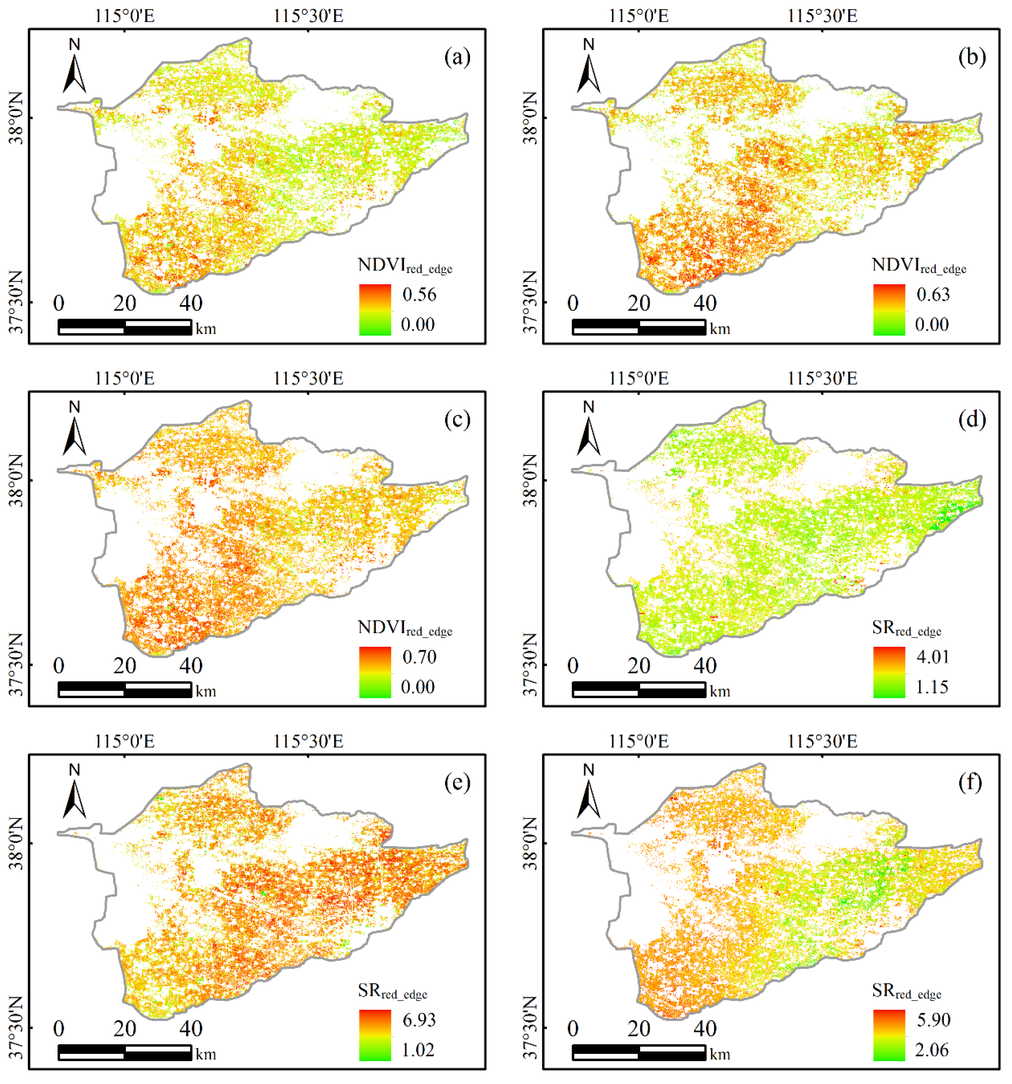
Figure 7.
The spatial distribution of the red-edge vegetation indices of crops in the main growing season. (a–c) Spatial distribution of NDVIred-edge of winter wheat from March to May. (d–f) Spatial distribution of SRred-edge of maize from July to September.
Figure 7.
The spatial distribution of the red-edge vegetation indices of crops in the main growing season. (a–c) Spatial distribution of NDVIred-edge of winter wheat from March to May. (d–f) Spatial distribution of SRred-edge of maize from July to September.

Figure 8.
The spatial distribution of the FPAR of crops in the main growing season. (a–c) Spatial distribution of the FPAR of winter wheat from March to May. (d–f) Spatial distribution of the FPAR of maize from July to September.
Figure 8.
The spatial distribution of the FPAR of crops in the main growing season. (a–c) Spatial distribution of the FPAR of winter wheat from March to May. (d–f) Spatial distribution of the FPAR of maize from July to September.

Figure 9.
The spatial distribution of the accumulated aboveground NPP and biomass of the crops during the main growing season. (a) Cumulative NPP of winter wheat from March to May. (b) Cumulative biomass of summer maize from July to September.
Figure 9.
The spatial distribution of the accumulated aboveground NPP and biomass of the crops during the main growing season. (a) Cumulative NPP of winter wheat from March to May. (b) Cumulative biomass of summer maize from July to September.


Figure 10.
The frequency of the accumulated NPP and biomass in the main growing seasons of the crops. (a,b) The frequency of the cumulative NPP of winter wheat and maize. (c,d) The frequency of the cumulative biomass of winter wheat and maize.
Figure 10.
The frequency of the accumulated NPP and biomass in the main growing seasons of the crops. (a,b) The frequency of the cumulative NPP of winter wheat and maize. (c,d) The frequency of the cumulative biomass of winter wheat and maize.


Figure 11.
Correlation of the aboveground biomass of winter wheat and maize in the main growing seasons.
Figure 11.
Correlation of the aboveground biomass of winter wheat and maize in the main growing seasons.

Figure 12.
Seasonal variations in NDVI, FPAR, LUE, and biomass in the main growing seasons. (a,b) Variations in the biophysical parameters of winter wheat and maize, respectively.
Figure 12.
Seasonal variations in NDVI, FPAR, LUE, and biomass in the main growing seasons. (a,b) Variations in the biophysical parameters of winter wheat and maize, respectively.

Figure 13.
Correlation between the predicted FPAR and the reference data in the main growing seasons. (a–h) Correlation between the FPAR retrieved by the NDVI, SR, MSR, EVI, , , , NDVI-SR, and MCD15A3H FPAR predictions.
Figure 13.
Correlation between the predicted FPAR and the reference data in the main growing seasons. (a–h) Correlation between the FPAR retrieved by the NDVI, SR, MSR, EVI, , , , NDVI-SR, and MCD15A3H FPAR predictions.


Figure 14.
Correlation histogram of the predicted FPAR of winter wheat and maize in the main growing seasons.
Figure 14.
Correlation histogram of the predicted FPAR of winter wheat and maize in the main growing seasons.

Figure 15.
Spatial distribution of seasonal average FPAR of different crops. (a–c) Seasonal average FPAR of winter wheat based on NDVIred-edge, NDVI and MODIS FPAR product. (d–f) Seasonal average FPAR of summer maize based on SRred-edge, NDVI and MODIS FPAR product.
Figure 15.
Spatial distribution of seasonal average FPAR of different crops. (a–c) Seasonal average FPAR of winter wheat based on NDVIred-edge, NDVI and MODIS FPAR product. (d–f) Seasonal average FPAR of summer maize based on SRred-edge, NDVI and MODIS FPAR product.

Figure 16.
Spatial distribution of aboveground biomass of different crops. (a–c) Aboveground biomass of winter wheat derived by improved CASA model, original CASA model and MODIS FPAR product. (d–f) Aboveground biomass of summer maize derived by improved CASA model, original CASA model and MODIS FPAR product.


Table 1.
Satellite data and descriptions.
| Satellite Data | Band | Center Wavelength (nm) | Resolution (m) | Source |
|---|---|---|---|---|
| Sentinel-2 | B1 | 443 | 60 | European Space Agency (https://sentinel.esa.int/web/sentinel/, accessed on 6 November 2020) |
| B2 | 490 | 10 | ||
| B3 | 560 | 10 | ||
| B4 | 665 | 10 | ||
| B5 | 705 | 20 | ||
| B6 | 740 | 20 | ||
| B7 | 783 | 20 | ||
| B8 | 842 | 10 | ||
| B8A | 865 | 20 | ||
| B9 | 940 | 60 | ||
| B10 | 1375 | 60 | ||
| B11 | 1610 | 20 | ||
| B12 | 2190 | 20 | ||
| QA10 | — | 10 | ||
| QA20 | — | 20 | ||
| QA60 | — | 60 | ||
| MCD15A3H | FPAR | — | 500 | NASA LP DAAC at the USGS EROS Center (https://lpdaac.usgs.gov/products/mcd15a3hv006/, accessed on 6 November 2020) |
| LAI | — | 500 |
Table 2.
Parameter values used for aboveground biomass estimation.
| Parameter | Unit | Description | Source |
|---|---|---|---|
| Meteorological Data | |||
| Temperature | °C | Near-surface (2 m) air temperature | China Meteorological Data Service Center (CMDSC) |
| Radiation | MJ/m2 | Surface downward shortwave radiation | Angstrom model |
| Measured Field Data | |||
| Winter Wheat Aboveground Biomass | g/m2 | Aboveground biomass at maturity stage | Field measurements |
| Summer Maize Aboveground Biomass | g/m2 | Aboveground biomass at maturity stage | Field measurements |
Table 3.
Regression accuracy of the FPAR of the red-edge vegetation indices.
| Crops | Vegetation Indices | Regression Model | R2 |
|---|---|---|---|
| Winter wheat | y = 0.8287x + 0.1889 | 0.72 | |
| y = 0.1656x + 0.7371 | 0.71 | ||
| y = 0.1619x + 0.0979 | 0.69 | ||
| Maize | y = 0.7081x − 0.0026 | 0.45 | |
| y = 0.1023x + 0.3011 | 0.53 | ||
| y = 0.5270x + 0.3305 | 0.40 |
Table 4.
Vegetation indices selected for the difference analysis. is the near-infrared band; is the red band; is the red-edge band.
Table 4.
Vegetation indices selected for the difference analysis. is the near-infrared band; is the red band; is the red-edge band.
| Vegetation Indices | Descriptions | Equation | Reference | |
|---|---|---|---|---|
| It corrects for some atmospheric conditions and canopy background noise. | (5) | [40] | ||
| It can distinguish green leaves from other objects and estimate the relative biomass. | (6) | [41] | ||
| It is used to assess vegetation biomass and growth, which reduces the impact of atmosphere and topography. | (7) | [42] | ||
| It is an improved version of SR, which is sensitive to vegetation biophysical parameters. | (8) | [43] | ||
| It uses bands in the red edge and incorporates a correction for leaf specular reflection. | (9) | [44] | ||
| It is similar to NDVI but capitalizes on the sensitivity of the vegetation red edge to small changes in canopy chlorophyll. | (10) | [45] | ||
| Combined with red band and near infrared band, it has strong robustness in a wide range. However, it saturates in dense vegetation conditions. | (11) | [46] | ||
Table 5.
Residual carbon ratio, dry matter ratio, and root–shoot ratio of crops.
| Crops | Carbon Content Ratio | Dry Matter Ratio | Root-Shoot Ratio | Moisture Content (%) | |
|---|---|---|---|---|---|
| Economic Production | Residual Carbon Ratio | ||||
| Winter wheat | 0.39 | 0.49 | 0.85 | 0.11 | 12.5 |
| Maize | 0.39 | 0.47 | 0.78 | 0.09 | 13.5 |
Publisher’s Note: MDPI stays neutral with regard to jurisdictional claims in published maps and institutional affiliations. |
© 2021 by the authors. Licensee MDPI, Basel, Switzerland. This article is an open access article distributed under the terms and conditions of the Creative Commons Attribution (CC BY) license (https://creativecommons.org/licenses/by/4.0/).
Share and Cite
MDPI and ACS Style
Fang, P.; Yan, N.; Wei, P.; Zhao, Y.; Zhang, X. Aboveground Biomass Mapping of Crops Supported by Improved CASA Model and Sentinel-2 Multispectral Imagery. Remote Sens. 2021, 13, 2755. https://0-doi-org.brum.beds.ac.uk/10.3390/rs13142755
AMA Style
Fang P, Yan N, Wei P, Zhao Y, Zhang X. Aboveground Biomass Mapping of Crops Supported by Improved CASA Model and Sentinel-2 Multispectral Imagery. Remote Sensing. 2021; 13(14):2755. https://0-doi-org.brum.beds.ac.uk/10.3390/rs13142755
Chicago/Turabian StyleFang, Peng, Nana Yan, Panpan Wei, Yifan Zhao, and Xiwang Zhang. 2021. "Aboveground Biomass Mapping of Crops Supported by Improved CASA Model and Sentinel-2 Multispectral Imagery" Remote Sensing 13, no. 14: 2755. https://0-doi-org.brum.beds.ac.uk/10.3390/rs13142755
Note that from the first issue of 2016, this journal uses article numbers instead of page numbers. See further details here.