Inversion of Geothermal Heat Flux under the Ice Sheet of Princess Elizabeth Land, East Antarctica

Abstract

Antarctic geothermal heat flux is a basic input variable for ice sheet dynamics simulation. It greatly affects the temperature and mechanical properties at the bottom of the ice sheet, influencing sliding, melting, and internal deformation. Due to the fact that the Antarctica is covered by a thick ice sheet, direct measurements of heat flux are very limited. This study was carried out to estimate the regional heat flux in the Antarctic continent through geophysical inversion. Princess Elizabeth Land, East Antarctica is one of the areas in which we have a weak understanding of geothermal heat flux. Through the latest airborne geomagnetic data, we inverted the Curie depth, obtaining the heat flux of bedrock based on the one-dimensional steady-state heat conduction equation. The results indicated that the Curie depth of the Princess Elizabeth Land is shallower than previously estimated, and the heat flux is consequently higher. Thus, the contribution of subglacial heat flux to the melting at the bottom of the ice sheet is likely greater than previously expected in this region. It further provides research clues for the formation of the developed subglacial water system in Princess Elizabeth Land.

1. Introduction

The Antarctic continent is covered by an ice sheet, which is a potential main driver of global sea-level changes. Heat flux of the bedrock significantly affects the melting of the ice sheet bottom, which may influence the ice sheet mass balance. Geothermal heat flux (GHF) is an important boundary condition of ice sheet dynamical models. For the areas below freezing point, a higher heat flux causes the ice bottom to heat up, reducing its viscosity and increasing its lubrication, and significantly accelerating the ice sheet flow [1]. Heat flux can also simulate past basic melting rates and help to explore the climate record of old ice cores [2]. Studies showed that East Antarctica has a smaller heat flux than the West Antarctica. This may be one of the reasons why the West Antarctic ice sheet is changing more rapidly [3]. However, some drilling results showed that the observed heat flux in some areas far exceeded the generally estimated heat flux by the GHF model [4,5,6]. The local subglacial thermal conditions have a greater impact on local ice sheet movement, which cannot be concealed by the low-resolution estimation results [7]. Recent studies showed that the surface mass loss of the ice sheet in Princess Elizabeth Land (PEL) is not as obvious as it is at the bottom [8]. The main contributing factor of the ice sheet material loss in this area may be obtained via ice sheet bottom analysis. Therefore, in order to more accurately model ice velocities and their evolution, and to learn more about the geology in PEL, it is necessary to obtain a more detailed understanding of the distribution of heat flux under the ice.

At present, there are three main methods for obtaining Antarctica heat flux information: (1) direct measurement of the geothermal gradient through ice boreholes or sediments on the coast [6,9,10]; (2) inversion by multiple geophysical methods, such as seismology, geomagnetism, and glacier dynamics [11,12,13,14,15]; and (3) using ice radar and the temperature gradient of the ice sheet or the ice bottom pressure melting point to calculate the distributions of heat flux [16,17]. Due to the rapid flow, ice sheet evolution is much faster than that of bedrock. However, it is difficult to calculate the thermal conditions of the ice bottom based on the temperature gradient of the ice sheet [17,18]. In addition, the ice sheet is very thick, and direct measurement of geothermal heat flux is very challenging [6]. Seismological methods estimate the subglacial thermal structure based on the thermal sensitivity of seismic properties. The disadvantage of this method is that the uneven distribution of seismic stations leads to the low resolution of seismic models, and many seismic parameters have significant uncertainties [15]. It is, therefore, a relatively common and efficient method to invert the heat flux through aerial geomagnetic observation.

Uncertainty surrounding the results obtained by the geomagnetic field mainly originate from the coverage of the data set and the reliability of the inversion method [1]. Available internationally in the public domain, the Antarctic magnetic data, known as the ADMAP2 data set, was released in 2018 and covers most of the Antarctica [19,20]. However, some areas still have large data gaps, especially in PEL, which was inverted by satellite magnetic data with a lower resolution. In the Martos Curie depth model [1], the maximum uncertainty value (~8 km) in this region is about 23% of the total Antarctic mean value (~34 km), which is higher than other regions.

2. Materials and Methods

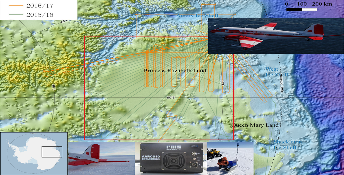
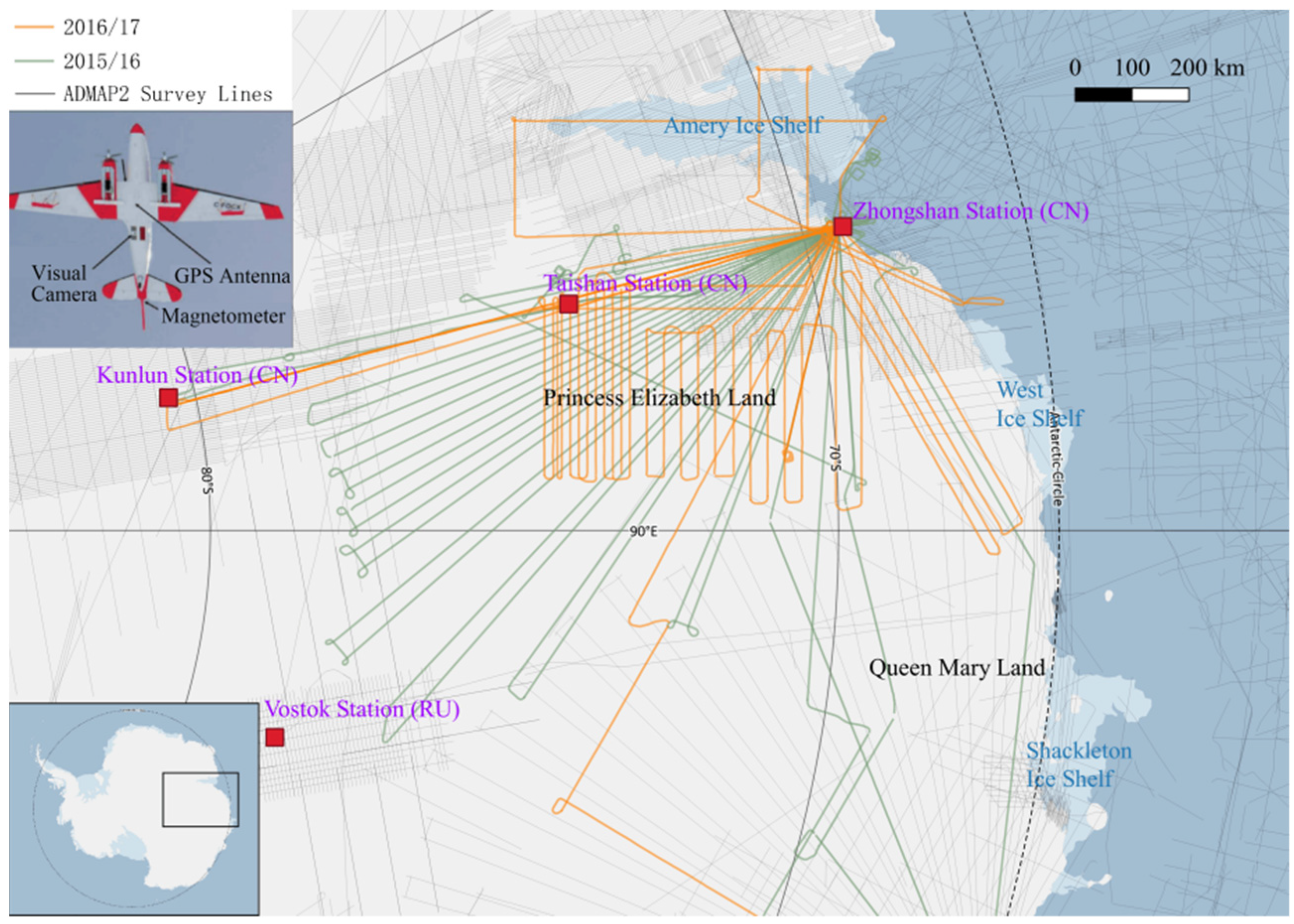
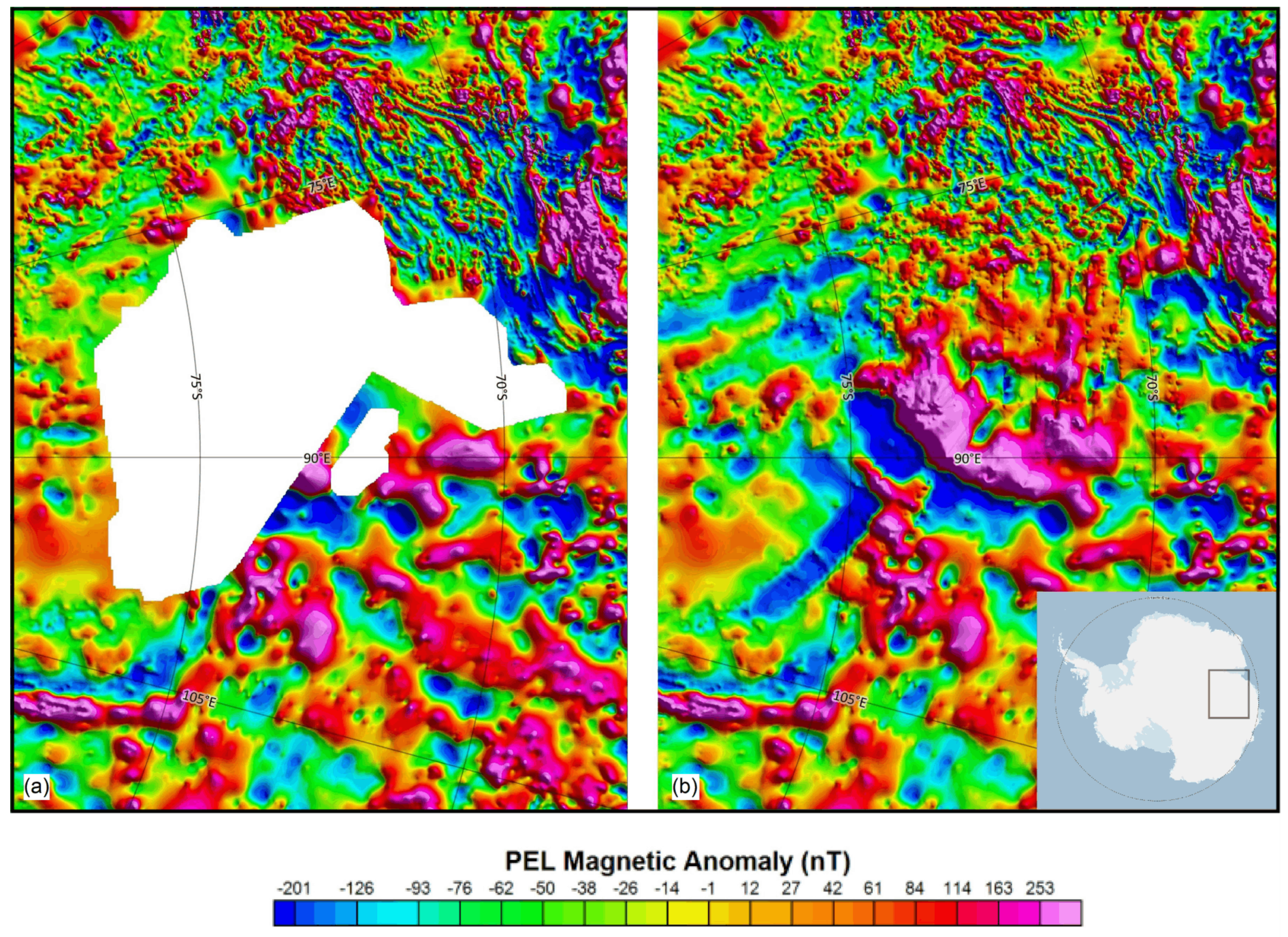
2.1. Aeromagnetic Data

Through the operation of China’s first Antarctic fixed-wing aircraft observation platform, we obtained large-scale aeromagnetic data from PEL. The single flight distance of the geophysical and glacier survey, carried out by the Snow Eagle 601 fixed-wing aircraft, was approximately 1700 km (6.5 h of endurance), and the total distance of the survey lines used in this study were about 47,000 km (Figure 1). During the aerial survey, flight altitude was maintained at 600 m above the ice surface.

The CS-3 magnetometer was used to measure the magnetic field. It was installed on the tail of the aircraft to avoid magnetic interference from the metal fuselage. The CS-3 magnetometer has high sensitivity and low noise interference, and its measurement range can be used for detection in most areas of the world. The magnetometer system consists of a Scintrex CS-3 scalar magnetometer, an RMS AARC510 adaptive aviation magnetic real-time compensator, and a Billingsley TFM100-G2 carrier magnetometer. During a survey, the CS-3 magnetometer measures the total magnetic field (with a sampling interval of 1 s, flight speed of 300 km/h, and sampling interval distance of ~83 m along the flight line), and the AARC510, with a three-axis fluxgate vector magnetometer, provides compensation for the influence of the flight direction and altitude.

The geomagnetic diurnal station (used for diurnal correction of the aeromagnetic survey) uses an EREV-1 proton magnetometer, located at the airport near the Zhongshan Station, with an absolute accuracy of less than 0.3 nT and a sampling interval of 1 s. In addition, a perennial geomagnetic observatory (with a sampling interval of 1 s) at the Zhongshan Station, 10 km away from the airport, provides backup data for diurnal observations.

We used the GRIDSTCH module of Oasis Montaj software for observational data fusion with ADMAP2. This method provides smooth blending without over-smoothing high-frequency variations that may occur along the suture path (Figure 2).

2.2. Inversion Method

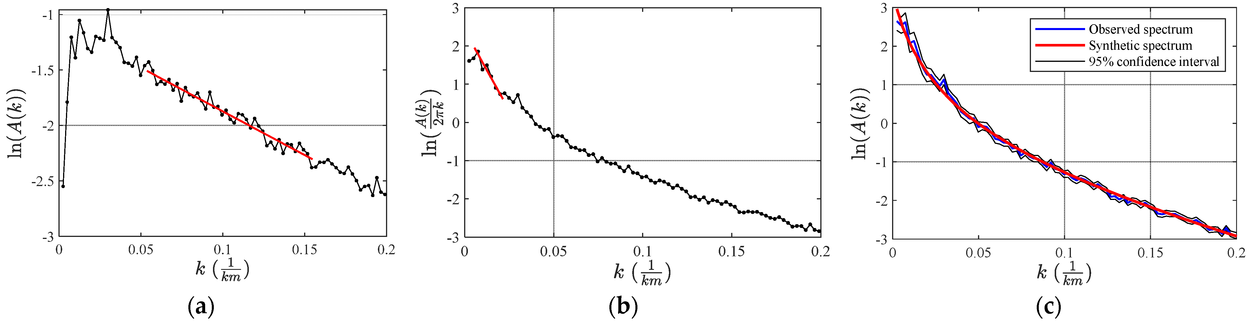
2.2.1. Using Modified Centroid Method to Invert the Curie Depth

The geomagnetic field is mainly produced in the ferromagnetic strata that exist in the Earth’s crust. After reaching a certain temperature, the ferromagnetic material will favor paramagnetism, which will significantly lower its magnetic field. At this temperature (580 °C for ferromagnetic ore [21]), the corresponding lithospheric interface is called the Curie isothermal interface, which is generally considered to be the bottom of the magnetic strata. Magnetic data can invert the large magnetic change interface and, thus, we can determine the Curie depth [22].

We used the centroid method to calculate the Curie depth. This method is based on the existence of a linear relationship between the spectral power density and specific wave number ranges. Compared with the defractal spectral method adopted by the Martos model, this method has very similar results under the same parameters [23]. In this method, it is assumed that the low wavenumber area of the power spectrum is caused by the deep field source, and the high wavenumber area is caused by the shallow field source. The Curie depth is considered to be the bottom interface of the deep field source, and, thus, it can be obtained through power spectrum analysis [24]:

$$\ln \left(A\left(k\right)\right)=E-\left|k\right|Z_t-\frac{\beta -1}{2}\ln \left|k\right|+\ln \left[1-e^{-\left|k\right|\left(Z_b-Z_t\right)}\right],$$

(1)

where A(k) is the radially averaged amplitude spectrum, and E is the constant related to the magnetization direction and geomagnetic field direction. First, we calculated the top surface depth of the deep field source. Then, we determined a fitting straight line from the high wavenumber region of the power spectrum, and calculated the depth of the deep field source top interface, $Z_t$, through the relationship with the slope of the straight line. Assuming $F$ is the constant, then Equation (1) is approximated to:

$$\ln \left(A\left(k\right)\right)\approx F-\left|k\right|Z_t-\frac{\beta -1}{2}\ln \left|k\right|,$$

(2)

Second, we calculated the depth of the centroid of the deep field source. We determined a fitting straight line from the low wavenumber region of the power spectrum, and calculated the centroid depth of the deep field source, $Z_0$, through the relationship with the slope of the straight line. Assuming $G$ is the constant:

$$\ln \left(A\left(k\right)/k\right)\approx G-\left|k\right|Z_0-\frac{\beta -1}{2}\ln \left|k\right|,$$

(3)

Finally, the depth of the bottom interface of the deep field source was calculated by the following simple positional relationship, calculating the Curie depth $Z_b$:

$$Z_b=2Z_0-Z_t,$$

(4)

The uncertainty associated with this method is calculated by [25]:

$$∆Z_b=\sqrt{2\times ∆{Z_0}^2+∆{Z_t}^2},$$

(5)

$∆Z_t$, $∆Z_0$ and $∆Z_b$ are the uncertainty of the top, the centroid, and the base of the magnetic source, respectively. The values of $∆Z_0$ and $∆Z_t$ were computed using the standard deviation (${\sigma }_r$) derived from the calculated power spectrum, and the linear fit in the wavenumber range was used to derive the slope ($k_2-k_1$) [26]. This uncertainty ($ϵ$) is:

$$ϵ=\frac{{\sigma }_r}{k_2-k_1},$$

(6)

For the division of the deep and the shallow field sources in the wavenumber range, manual intervention must be processed using digital methods, instead of automatic division, to reduce the error. Since the fractal parameters $\beta$ are unknown, in the case of wavenumber range participating in the matching has been determined, the observed power spectrum and the random magnetization model power spectrum can be optimally matched by continuously adjusting $\beta$ (with an adjustment interval of 0.1). Only then will the $\beta$ reflect the geological structure more truly.

The goodness of fit is evaluated using the following equation [23]:

$$R=\sqrt{\frac{1}{n}{{\displaystyle \sum }}_{i=1}^n{\left(A_f\left(k\right)-A_{syn}\left(k\right)\right)}^2},$$

(7)

where $A_f\left(k\right)$ is the observed power spectrum and $A_{syn}\left(k\right)$ is the model power spectrum. The smaller the R value, the better the fit. Manual adjustment is required in the process of adjusting the wavenumber range and $\beta$, which can reduce the uncertainty related to $\beta$.

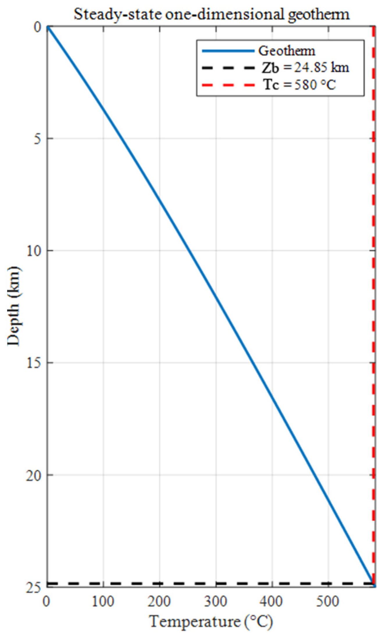
2.2.2. Calculating the Geothermal Heat Flux Based on Curie Depth

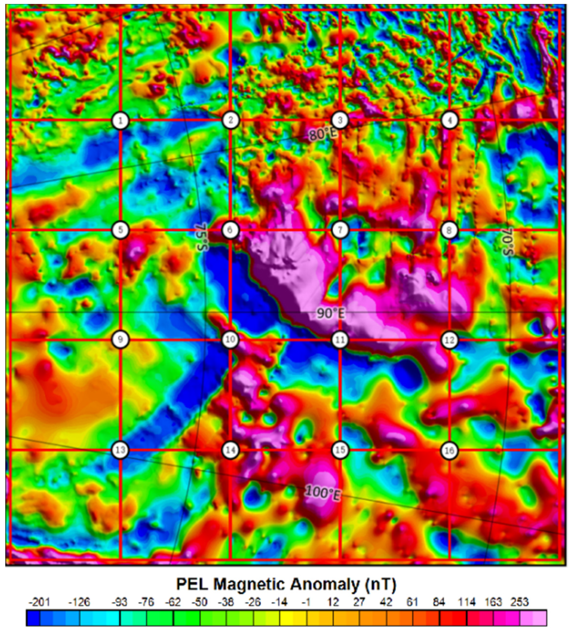
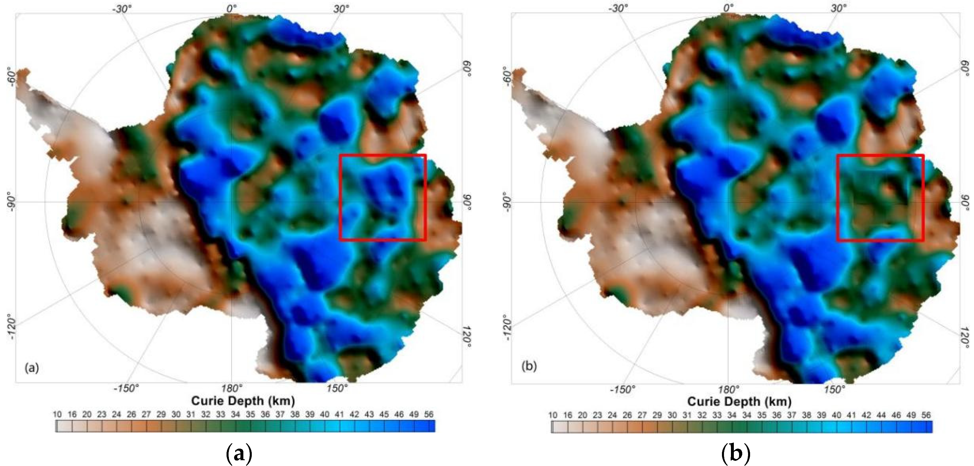
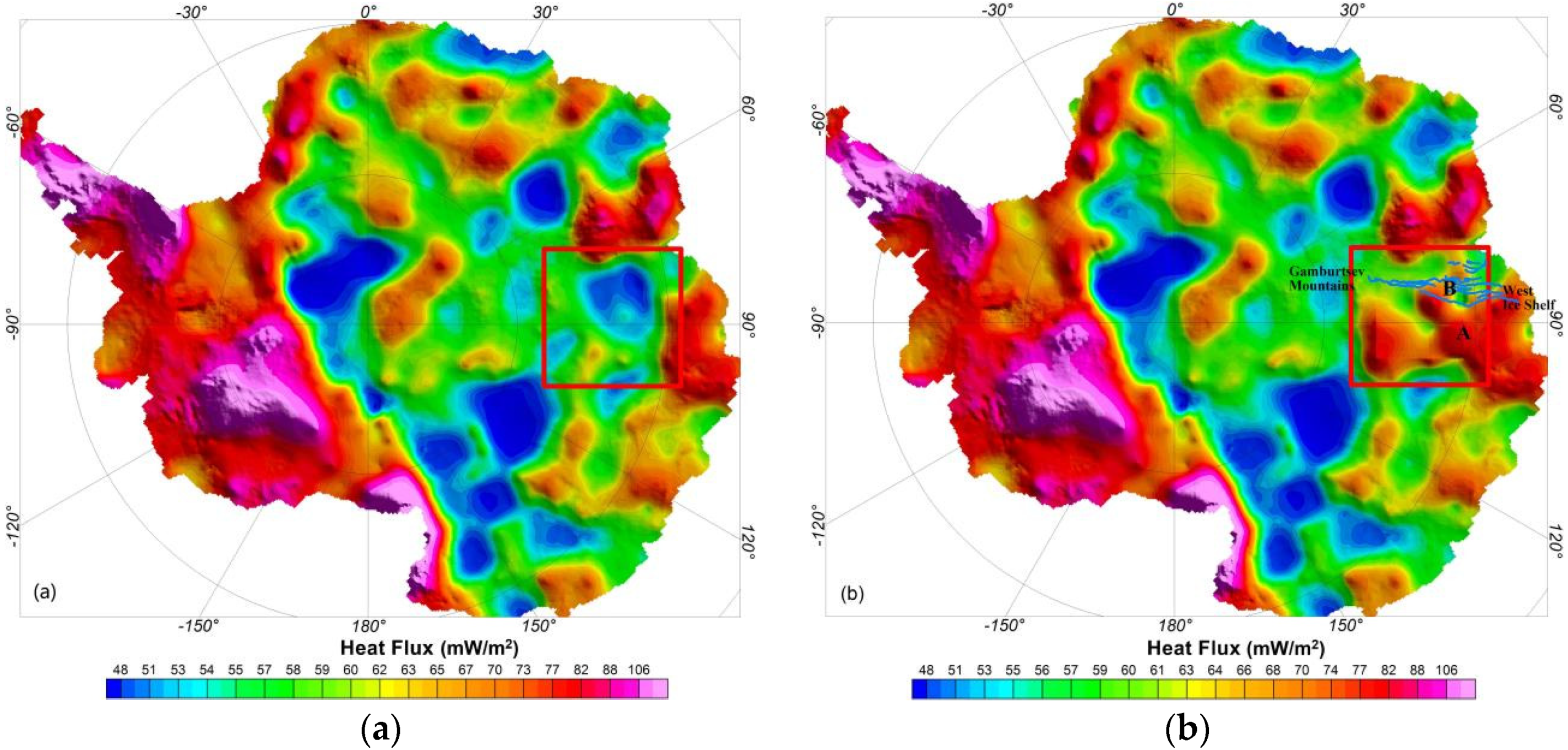
The relationship between the Curie depth and geothermal gradient can be approximated by the one-dimensional steady-state heat conduction equation, which can calculate the approximate geothermal heat flux of the Antarctic subglacial bedrock.

Assuming that there is no lateral heat production and conduction in the bedrock under the ice sheet, and that the longitudinal thermal conductivity is constant, if $q$ is heat flux, $z$ is depth, $\lambda$ is thermal conductivity, and $T$ is temperature, then the one-dimensional steady-state heat conduction equation will be:

$$q\left(z\right)=\lambda \frac{\partial T\left(z\right)}{\partial z},$$

(8)

Assuming that $Z_b$ is Curie depth, $T_c$. is Curie temperature, $T_0$. is surface temperature, $H_0$ is the surface heat production, $h_r$ is the depth for heat production, and $q_s$ is the surface geothermal heat flux, the heat conduction equation will be [27,28,29]:

$$q_s=\frac{\lambda \left(T_c-T_0\right)}{Z_b}+H_0{h}_r-\frac{H_0{h}_r^2}{Z_b}\left(1-e^{\left(-Z_b/h_r\right)}\right),$$

(9)

3. Results

According to the previous approximate distribution of the Curie depth inversion results for magnetic data in the Antarctica [1], we divided the observation area into 16 windows and calculated the Curie depth separately in each window. The size of each window was set to 400 × 400 km, which meant a 50% overlap between adjacent windows, as shown in Figure 3. The calculation result of each window corresponded to the center point. After data fusion, each piece of data was processed according to the larger spacing grid of ADMAP2 (1.5 km spacing) to ensure data accuracy.

In Figure 4, using window 3 as an example, the process of artificially dividing the wavenumber ranges, the fitting state of the observed power spectrum, and the simulated power spectrum are shown.

According to the radial power spectrum of PEL, the high wavenumber range is generally concentrated between 0.05 and 0.15, and the low wavenumber range is concentrated between 0.01 and 0.03. The difference between the observed power spectrum and the simulated power spectrum R was between 0.05 and 0.15.

In the process of calculating the heat flux from the Curie depth, the selection of geothermal parameters refers to the previous inference results [1]. It is generally believed that the surface temperature, $T_0$, is ~0 °C, the surface heat production, $H_0$, is ~2.5 mW/m³, the thermal conductivity, $\lambda$, is ~2.8 W/mK, and the depth for heat production, $h_r$, is ~8 km [30]. The Curie temperature, $T_c$, refers to a constant value of 580 °C. According to the Curie depth results, 16 areas were combined with the one-dimensional steady-state heat conduction equation to calculate the geothermal gradient and heat flux. Using window 3 as an example, the calculation results of regional geothermal gradient and heat flux are shown in Figure 5.

The combined calculation results of the Curie depth and the heat flux with the previous calculation results of the all-Antarctica magnetic field [1] are compared in Figure 6 and Figure 7.

The Curie depth range of East Antarctica in the Martos model was from 22 to 63 km. From our inversion results, the Curie depth of PEL was observed to be shallower than previously estimated depths, most of which varied in the range of 23–48 km, with an average depth of about 34 km, and a calculation error of ±4 km. The heat flux map showed that Queen Mary Land (Label A in Figure 7b) had the same magnitude of high geothermal heat flux as the region closer to the western ice shelf, which is consistent with the previous seismic model inversion results [31,32]. Overall, the heat flux was larger than previously estimated in the eastern area of PEL. Figure 7 indicates values ranging from 51 to 84 mW/m², with an average of 66 mW/m² and an error of ±7 mW/m², which is close to the global continental average of 65 mW/m² [7]. By comparison, the model of Martos et al. had a heat flow value of 45–85 mW/m² in East Antarctica [1], which is slightly lower than our calculation result.

4. Discussion

Previous satellite altimetry studies showed that there is an undiscovered, large sub-glacial drainage network hidden under the ice sheet of PEL. A series of long, deep canyons from Gamburtsev Mountain extend to the coast of the West Ice Shelf (Label B in Figure 7b). These canyons contain large amounts of subglacial water and lakes [33]. The aerial ice radar detection results of Snow Eagle 601 also confirmed this conclusion [34,35]. The North-South rift zones were formed during the Cenozoic crustal uplift and through volcanism in the area [7,36,37]. The rift system is believed to be an area where the geothermal heat flux is significantly increased [38]. In our calculation results, there is a high-low-high change trend in this area. In the process of rift formation, the influence of complex tectonism on the surrounding strata, such as the formation of metamorphic rocks caused by ductile shear zone and nappe structure, can be used to explain the origin of high and low heat flux in this area [39,40]. The high heat flux region described by this study (Figure 7b) may represent the product of orogeny and rift extension, as well as possible “thermal events” [41] during the evolution of the Antarctic continent [42,43].

Furthermore, there is a clear correlation between the subglacial water system and the heat flux [44,45]. Temperature profile analysis in ice boreholes showed that the bedrocks are warm at sites where subglacial water exists [18]. Geothermal heat flux of 120 ± 20 mW/m² can cause basal melting of up to 6 ± 1 mm/a [46]. Jamieson believed that the canyons reduced the likelihood of rapid ice flow due to the fact that rather than concentrating the water at one point and enhancing the sliding of the ice bottom, they capturing the water body so it cannot lubricate the ice-bed interface over a wide area [33]. The detailed distribution of water bodies under ice need to be analyzed by calculation of ice radar reflectivity. The heat flux distribution in this study may encourage further explanation of the distribution and cause of the subglacial water system in this area.

In general, the geomagnetic method is an efficient method for estimating heat flux. The inversion of the Curie depth, however, induces error due to the assumption of structural division, and it becomes difficult to divide the low wavenumber range, which represents the deep magnetic field source. The calculation of heat flux may also contain some errors due to the uneven heat production. The survey line spacing in the southeastern part of the study area close to Vostok is relatively large. It is greater than 100 km at the widest point, which may cause an error of more than 10 km in the estimation of the Curie depth. In order to improve the calculation results, it is necessary to carry out further survey lines of airborne geophysical observation and deeper borehole measurements. An integrated study of the regional geological structure of PEL in combination with geophysical inversion would provide more accurate information about the subglacial thermal environment in this region.

5. Conclusions

Based on the aeromagnetic data of PEL obtained by China’s fixed-wing aircraft observation platform, and by using the modified centroid method and the one-dimensional steady-state heat conduction equation, we obtained geothermal heat flux data on PEL’s ice sheet bottom. The Curie depth result was shallower than previously estimated and the heat flux was higher, showing that the contribution of subglacial heat flux to the melting of the ice sheet in this area is greater than previously calculated, which may be an important reason for the development of the subglacial water system in PEL.

Our calculation results showed that the high geothermal heat flux is better correlated with the melting of the bottom ice and the distribution of water in this area. GHF inference provided relatively accurate boundary conditions for simulating the dynamics and evolution of the ice sheet, which may help in estimating the bottom melting rate of the East Antarctic ice sheet and its impact on sea-level rise.

References

1. Martos, Y.M.; Catalán, M.; Jordan, T.A.; Golynsky, A.; Golynsky, D.; Eagles, G.; Vaughan, D.G. Heat Flux Distribution of Antarctica Unveiled. Geophys. Res. Lett. 2017, 44, 11417–11426. [Google Scholar] [CrossRef] [Green Version]
2. Burton-Johnson, A.; Dziadek, R.; Martin, C.; Halpin, J.; Whitehouse, P.L.; Ebbing, J.; Martos, Y.M.; Martin, A.; Schroeder, D.; Shen, W.; et al. Antarctic Geothermal Heat Flow: Future Research Directions; EPIC3SCAR-SERCE White Paper; Scientific Committee on Antarctic Research (SCAR): Paris, France, 2020; Volume 2006, pp. 1–9. [Google Scholar]
3. Llubes, M.; Lanseau, C.; Rémy, F. Relations between basal condition, sub-glacial hydrological networks and geothermal flux in Antarctica. Earth Planet. Sci. Lett. 2006, 241, 655–662. [Google Scholar] [CrossRef]
4. Risk, G.F.; Hochstein, M.P. Heat flow at arrival heights, Ross Island, Antarctica. N. Z. J. Geol. Geophys. 1974, 17, 629–644. [Google Scholar] [CrossRef]
5. Morin, R.H.; Williams, T.; Henrys, S.A.; Magens, D.; Niessen, F.; Hansaraj, D. Heat flow and hydrologic characteristics at the AND-1B borehole, ANDRILL McMurdo ice shelf project, Antarctica. Geosphere 2010, 6, 370–378. [Google Scholar] [CrossRef] [Green Version]
6. Fisher, A.T.; Mankoff, K.D.; Tulaczyk, S.M.; Tyler, S.W.; Foley, N. High geothermal heat flux measured below the West Antarctic ice sheet. Sci. Adv. 2015, 1, e1500093. [Google Scholar] [CrossRef] [PubMed] [Green Version]
7. Pollack, H.N.; Hurter, S.J.; Johnson, J.R. Heat flow from the earth’s interior: Analysis of the global data set. Rev. Geophys. 1993, 31, 267–280. [Google Scholar] [CrossRef]
8. Yamane, M.; Yokoyama, Y.; Abe-Ouchi, A.; Obrochta, S.; Saito, F.; Moriwaki, K.; Matsuzaki, H. Exposure age and ice-sheet model constraints on Pliocene East Antarctic ice sheet dynamics. Nat. Commun. 2015, 6, 7016. [Google Scholar] [CrossRef] [PubMed]
9. Engelhardt, H. Ice temperature and high geothermal flux at Siple Dome, west Antarctica, from borehole measurements. J. Glaciol. 2004, 50, 251–256. [Google Scholar] [CrossRef] [Green Version]
10. Hasterok, D. Thermal State of Continental and Oceanic Lithosphere. Ph.D. Thesis, University of Utah, Salt Lake City, UT, USA, 2010; p. 167. [Google Scholar]
11. Dalziel, I.W.; Elliot, D.H. West Antarctica: Problem child of Gondwanaland. Tectonics 1982, 1, 3–19. [Google Scholar] [CrossRef]
12. Block, A.E.; Bell, R.E.; Studinger, M. Antarctic crustal thickness from satellite gravity: Implications for the transantarctic and Gamburtsev Subglacial Mountains. Earth Planet. Sci. Lett. 2009, 288, 194–203. [Google Scholar] [CrossRef]
13. Fretwell, P.; Pritchard, H.D.; Vaughan, D.G.; Bamber, J.L.; Barrand, N.E.; Bell, R.; Zirizzotti, A. Bedmap2: Improved ice bed, surface and thickness datasets for Antarctica. Cryosphere 2013, 7, 375–393. [Google Scholar] [CrossRef] [Green Version]
14. An, M.; Wiens, D.A.; Zhao, Y.; Feng, M.; Nyblade, A.A.; Kanao, M.; Lévêque, J.J. S-velocity model and inferred Moho topography beneath the Antarctic plate from Rayleigh waves. J. Geophys. Res. Solid Earth 2015, 120, 359–383. [Google Scholar] [CrossRef]
15. Shen, W.; Wiens, D.A.; Lloyd, A.J.; Nyblade, A.A. A Geothermal Heat Flux Map of Antarctica Empirically Constrained by Seismic Structure. Geophys. Res. Lett. 2020, 47, e2020GL086955. [Google Scholar] [CrossRef]
16. Wolovick, M.J.; Moore, J.C.; Zhao, L. Joint Inversion for Surface Accumulation Rate and Geothermal Heat Flow From Ice-Penetrating Radar Observations at Dome A, East Antarctica. Part I: Model Description, Data Constraints and Inversion Results. J. Geophys. Res. Earth Surf. 2021, 126, 1–27. [Google Scholar] [CrossRef]
17. Zagorodnov, V.; Nagornov, O.; Scambos, T.A.; Muto, A.; Mosley-Thompson, E.; Pettit, E.C.; Tyuflin, S. Borehole temperatures reveal details of 20th century warming at Bruce Plateau, Antarctic Peninsula. Cryosphere 2012, 6, 675–686. [Google Scholar] [CrossRef] [Green Version]
18. Talalay, P.; Li, Y.; Augustin, L.; Clow, G.D.; Hong, J.; Lefebvre, E.; Markov, A.; Motoyama, H.; Ritz, C. Geothermal heat flux from measured temperature profiles in deep ice boreholes in Antarctica. Cryosphere 2020, 14, 4021–4037. [Google Scholar] [CrossRef]
19. Golynsky, A.V.; Ferraccioli, F.; Hong, J.K.; Golynsky, D.A.; von Frese, R.R.B.; Young, D.A.; Blankenship, D.D.; Holt, J.W.; Ivanov, S.V.; Kiselev, A.V.; et al. ADMAP2 Magnetic anomaly map of the Antarctic—links to files. PANGAEA 2018. [Google Scholar] [CrossRef]
20. Golynsky, A.V.; Ferraccioli, F.; Hong, J.K.; Golynsky, D.A.; von Frese, R.R.B.; Young, D.A.; Blankenship, J.W.; Holt, S.V.; Ivanov, A.V.; Kilesev, V.N.; et al. New magnetic anomaly map of the Antarctic. Geophys. Res. Lett. 45, 6437–6449. [CrossRef]
21. Frost, B.R.; Shive, P.N. Magnetic mineralogy of the lower continental crust. J. Geophys. Res. Atmos. 1986, 91, 6513–6521. [Google Scholar] [CrossRef]
22. Tanaka, A.; Okubo, Y.; Matsubayashi, O. Curie point depth based on spectrum analysis of the magnetic anomaly data in East and Southeast Asia. Tectonophysics 1999, 306, 461–470. [Google Scholar] [CrossRef]
23. Carrillo-de la Cruz, J.L.; Prol-Ledesma, R.M.; Velázquez-Sánchez, P.; Gómez-Rodríguez, D. MAGCPD: A MATLAB-based GUI to calculate the Curie point-depth involving the spectral analysis of aeromagnetic data. Earth Sci. Inform. 2020, 13, 1539–1550. [Google Scholar] [CrossRef]
24. Spector, A.; Grant, F.S. Statistical model for interpreting aeromagnetric data. Geophysics 1970, 35, 293–302. [Google Scholar] [CrossRef]
25. Martos, Y.M.; Catalán, M.; Galindo-Zaldivar, J. Curie depth, heat flux and thermal subsidence reveal the Pacific mantle outflow through the Scotia Sea. J. Geophys Res. Solid Earth 2019, 124, 10735–10751. [Google Scholar] [CrossRef]
26. Okubo, Y.; Matsunaga, T. Curie point depth in Northeast Japan and its correlation with regional thermal structure and seismicity. J. Geophys. Res. 1994, 99, 22363–22371. [Google Scholar] [CrossRef]
27. Birch, F.; Roy, R.F.; Decker, E.R. Heat flow and thermal history in New England and New York. In Studies of Appalachian Geology: Northern and Maritime; Zen, E.-A., Ed.; Wiley Interscience: New York, NY, USA, 1968; pp. 437–451. [Google Scholar]
28. Lachenbruch, A.H. Preliminary geothermal model of the Sierra Nevada. J. Geophys. Res. 1968, 73, 6977–6989. [Google Scholar] [CrossRef]
29. Roy, R.F.; Blackwell, D.D.; Birch, F. Heat generation of plutonic rocks and continental heat flow provinces. Earth Planet. Sci. Lett. 1968, 5, 1–12. [Google Scholar] [CrossRef]
30. Ravat, D.; Morgan, P.; Lowry, A.R. Geotherms from the temperature- depth–constrained solutions of 1-D steady-state heat-flow equation. Geosphere 2016, 12, 1187–1197. [Google Scholar] [CrossRef]
31. Shapiro, N.M.; Ritzwoller, M.H. Inferring surface heat flux distributions guided by a global seismic model: Particular application to Antarctica. Earth Planet. Sci. Lett. 2004, 223, 213–224. [Google Scholar] [CrossRef] [Green Version]
32. An, M.; Wiens, D.A.; Zhao, Y.; Feng, M.; Nyblade, A.; Kanao, M.; Li, Y.; Maggi, A.; Lévêque, J.-J. Temperature, lithosphere-asthenosphere boundary, and heat flux beneath the Antarctic Plate inferred from seismic velocities. J. Geophys. Res. Solid Earth 2015, 120, 8720–8742. [Google Scholar] [CrossRef]
33. Jamieson, S.S.R.; Ross, N.; Greenbaum, J.S.; Young, D.A.; Aitken, A.R.A.; Roberts, J.L.; Blankenship, D.D.; Bo, S.; Siegert, M.J. An extensive subglacial lake and canyon system in Princess Elizabeth Land, East Antarctica. Geology 2016, 44, 87–90. [Google Scholar] [CrossRef] [Green Version]
34. Cui, X.; Greenbaum, J.S.; Beem, L.H.; Guo, J.; Ng, G.; Li, L.; Blankenship, D.; Sun, B. The First Fixed-wing Aircraft for Chinese Antarctic Expeditions: Airframe, Modifications, Scientific Instrumentation and Applications. J. Environ. Eng. Geophys 2018, 23, 1–13. [Google Scholar] [CrossRef]
35. Cui, X.; Jeofry, H.; Greenbaum, J.S.; Guo, J.; Li, L.; Lindzey, L.E.; Habbal, F.A.; Wei, W.; Young, D.A.; Ross, N.; et al. Bed topography of Princess Elizabeth Land in East Antarctica. Earth Syst. Sci. Data 2020, 12, 2765–2774. [Google Scholar] [CrossRef]
36. LeMasurier, W.E.; Thomson, J.W. (Eds.) Volcanoes of the Antarctic plate and Southern Oceans. In Antarctic Research Series; American Geophysical Union: Washington, DC, USA, 1990; Volume 48, p. 487. [Google Scholar]
37. Hambrey, M.J.; McKelvey, B. Major Neogene fluctuations of the East Antarctic ice sheet: Stratigraphic evidence from the Lambert glacier region. Geology 2000, 28, 887–890. [Google Scholar] [CrossRef]
38. Morgan, P. Constraints on rift thermal processes from heat flow and uplift. Tectonophysics 1983, 94, 277–298. [Google Scholar] [CrossRef]
39. Liu, X.; Wang, W.; Zhao, Y.; Liu, J.; Chen, H.; Cui, Y.; Song, B. Early Mesoproterozoic arc magmatism followed by early Neoproterozoic granulite facies metamorphism with a near-isobaric cooling path at Mount Brown, Princess Elizabeth Land, East Antarctica. Precambrian Res. 2016, 284, 30–48. [Google Scholar] [CrossRef]
40. Pollett, A.; Thiel, S.; Bendall, B.; Raimondo, T.; Hand, M. Mapping the Gawler Craton–Musgrave Province interface using integrated heat flow and magnetotellurics. Tectonophysics 2019, 756, 43–56. [Google Scholar] [CrossRef]
41. Liu, X.; Yue, Z.; Hong, C.; Song, B. New zircon U–Pb and Hf–Nd isotopic constraints on the timing of magmatism, sedimentation and metamorphism in the northern Prince Charles Mountains, East Antarctica. Precambrian Res. 2017, 299, 15–33. [Google Scholar] [CrossRef]
42. Mueller, S.G.; Krapez, B.; Barley, M.E.; Fletcher, I.R. Giant iron-ore deposits of the Hamersley Province related to the breakup of Paleoproterozoic Australia; new insights from in situ SHRIMP dating of baddeleyite from mafic intrusions. Geology 2005, 33, 577–580. [Google Scholar] [CrossRef]
43. Rogers, J.; Santosh, M. Tectonics and surface effects of the supercontinent Columbia. Gondwana Res. 2009, 15, 373–380. [Google Scholar] [CrossRef]
44. Schroeder, D.M.; Blankenship, D.D.; Young, D.A.; Quartini, E. Evidence for elevated and spatially variable geothermal flux beneath the West Antarctic Ice Sheet. Proc. Natl. Acad. Sci. USA 2014, 111, 9070–9072. [Google Scholar] [CrossRef] [Green Version]
45. Dziadek, R.; Gohl, K.; Diehl, A.; Kaul, N. Geothermal heat flux in the Amundsen Sea sector of West Antarctica: New insights from temperature measurements, depth to the bottom of the magnetic source estimation and thermal modeling. Geochem. Geophys. Geosyst. 2017, 18, 2657–2672. [Google Scholar] [CrossRef]
46. Jordan, T.A.; Martin, C.; Ferraccioli, F.; Matsuoka, K.; Corr, H.; Forsberg, R.; Olesen, A.; Siegert, M. Anomalously high geothermal flux near the South Pole. Sci. Rep. 2018, 8, 1–8. [Google Scholar] [CrossRef] [PubMed] [Green Version]
Figure 1. Snow Eagle 601 aeromagnetic survey lines.
Remotesensing 13 02760 g001
Figure 2. Comparison of aeromagnetic data from Snow Eagle 601 observation platform with ADMAP2 magnetic data. The (a) ADMAP2 data set (note that there is no data in the blank area), and the (b) data set after fusion of the aeromagnetic data obtained by Snow Eagle 601 fixed-wing aircraft.
Remotesensing 13 02760 g002
Figure 3. Princess Elizabeth Land block divisions for calculation. Taking the marked position (white circle) as the center, the size of each window is 400 × 400 km, and the adjacent windows have a 50% overlapping coverage rate. There are 16 square windows in total covering PEL.
Remotesensing 13 02760 g003
Figure 4. The dividing the wave number range and determination of the fractal parameters, using window 3 as an example, according to the fitted curve. The (a) selected high wavenumber range; (b) selected low wavenumber range; and (c) degree of fit between the observed power spectrum and the simulated power spectrum.
Remotesensing 13 02760 g004
Figure 5. The inversion result of the ground temperature gradient using window 3 as an example.
Remotesensing 13 02760 g005
Figure 6. Comparison of Curie depth maps. The (a) previous calculation results of all Antarctica [1]; and (b) combining our calculation results in PEL (red frame area).
Remotesensing 13 02760 g006
Figure 7. Comparison of heat flux maps. The (a) previous calculation results of all Antarctica [1], and (b) combining our calculation results in PEL (red frame area). Blue lines indicate the location of rifts.
Remotesensing 13 02760 g007
Publisher’s Note: MDPI stays neutral with regard to jurisdictional claims in published maps and institutional affiliations.