
Learning the Incremental Warp for 3D Vehicle Tracking in LiDAR Point Clouds


1
School of Mathematical Sciences, Dalian University of Technology, Dalian 116024, China
2
School of Computer and Technology, Shan Dong Jianzhu University, Jinan 250101, China
3
Discipline of Business Analytics, Business School, The University of Sydney, Sydney, NSW 2006, Australia
4
Faculty of Electronic Information and Electrical Engineering, Dalian University of Technology, Dalian 116024, China
*
Author to whom correspondence should be addressed.
Remote Sens. 2021, 13(14), 2770; https://0-doi-org.brum.beds.ac.uk/10.3390/rs13142770
Submission received: 24 June 2021
/
Revised: 9 July 2021
/
Accepted: 9 July 2021
/
Published: 14 July 2021
(This article belongs to the Special Issue Deep Learning and Computer Vision in Remote Sensing)
Abstract
:Object tracking from LiDAR point clouds, which are always incomplete, sparse, and unstructured, plays a crucial role in urban navigation. Some existing methods utilize a learned similarity network for locating the target, immensely limiting the advancements in tracking accuracy. In this study, we leveraged a powerful target discriminator and an accurate state estimator to robustly track target objects in challenging point cloud scenarios. Considering the complex nature of estimating the state, we extended the traditional Lucas and Kanade (LK) algorithm to 3D point cloud tracking. Specifically, we propose a state estimation subnetwork that aims to learn the incremental warp for updating the coarse target state. Moreover, to obtain a coarse state, we present a simple yet efficient discrimination subnetwork. It can project 3D shapes into a more discriminatory latent space by integrating the global feature into each point-wise feature. Experiments on KITTI and PandaSet datasets showed that compared with the most advanced of other methods, our proposed method can achieve significant improvements—in particular, up to 13.68% on KITTI.
1. Introduction
Single object tracking in point clouds aims to localize the time-varying target represented by point clouds with the supervision of a 3D bounding box in the first frame. It is a challenging yet indispensable task in many real-world applications, such as autonomous driving [1,2] and mobile robot tracking [3,4]. Generally, object tracking encompasses two subtasks, target discrimination and state estimation, which are the fundamental steps for an agent to sense the surrounding environment and conduct motion planning [5]. Over the last few years, 2D single object tracking task has been explored extensively [6,7,8,9]. Inspired by that success, many RGB-D based methods refer to the pattern of 2D tracking to conduct 3D tracking [10,11,12,13]. Although working well in the conventional 2D domain, these methods rely heavily on the RGB modality. They hence may fail when color information is low-quality or even unavailable. In this work, we focus on the 3D vehicle tracking task using deep learning in point clouds, which is still in the development stage due to several factors, such as self-occlusion, disorder, density change, and the difficulty of the state estimation.
Recently, the high-end sensors for LiDAR (light detection and ranging) have attracted much attention, since they have high accuracy and are less sensitive to weather conditions than most other sensors. More importantly, it can capture the structure of a scene by producing plenty of 3D point clouds to provide reliable geometric information from far away. However, the source data constitute the unstructured representation, where the standard convolution operation is not applicable. This hampers the application of deep learning models in 3D object tracking. To overcome this barrier, some studies projected point clouds onto planes from a bird’s-eye view (BEV), and then discretized them into 2D images [5,14,15].
Although they could conduct tracking by detecting frame by frame, the BEV loses abundant geometric information. Consequently, starting from source point clouds, Giancola et al. [2] proposed SiamTrack3D to learn a generically template matching function which is trained by the shape completion regularization. Qi et al. [16] leveraged deep Hough voting [17] to produce potential bounding boxes. It is worth mentioning that the aforementioned approaches merely focus on determining the best proposal from a set of object proposals. In other words, they thoroughly ignore the importance of comprehensively considering both the target discrimination and the state estimation [18].
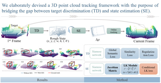
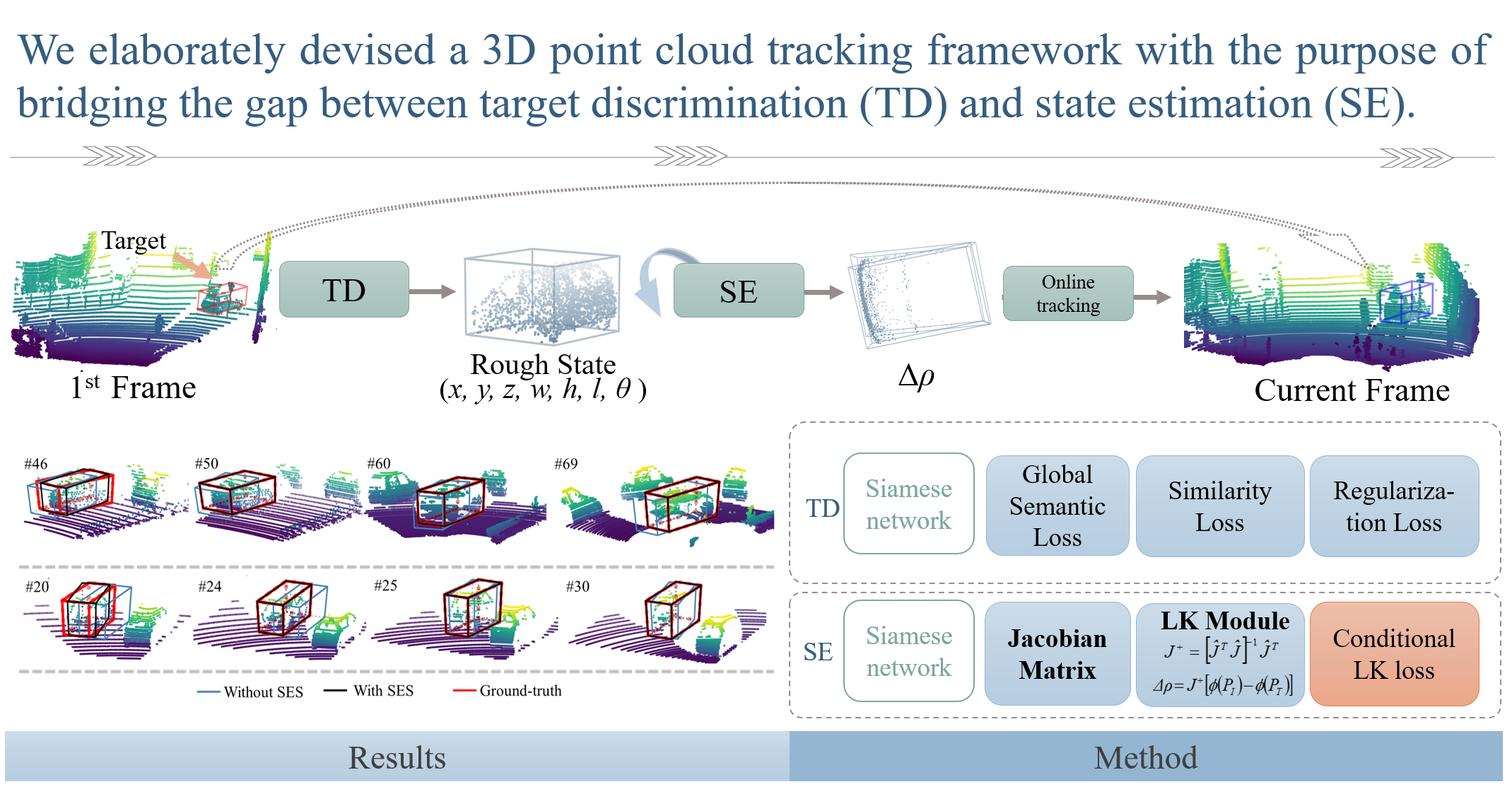
To address this problem, we elaborately designed a 3D point cloud tracking framework with the purpose of bridging the gap between target discrimination and state estimation. It is mainly comprised of two components, a powerful target discriminator and an accurate target state estimator, which realize their respective functions through the Siamese network. The state estimation subnetwork (SES) is proposed to estimate a optimal warp using the template and candidates extracted from the tracked frame. This subnetwork extends the 2D Lucas and Kanade (LK) algorithm [19] to the 3D point cloud tracking problem by incorporating it into a deep network. However, it is non-trivial, since the Jacobian matrix from the first-order Taylor expansion cannot be calculated as in the RGB image, where the Jacobian matrix can be split into two partial terms using the chain rule. The reason is that the gradients in x, y, and z cannot be calculated, as connections among points are lacking in 3D point clouds. To circumvent this issue, we thoughtfully present an approximation-based solution and a learning-based solution. By integrating them into a deep network in an end-to-end manner, our state estimation subnetwork can take a pair of point clouds as inputs to predict the incremental warp parameters. Additionally, we introduce an efficient target discrimination subnetwork (TDS) to remedy the deficiency of the SES. In order to project 3D shapes into a more discriminatory latent space, we designed a new loss that takes global semantic information into consideration. During online tracking, by forcing these two components to cooperate with each other properly, our proposed model could cope with the challenging point cloud scenarios robustly.
The key contributions of our work are three-fold:
- A novel state estimation subnetwork was designed, which extends the 2D LK algorithm to 3D point cloud tracking. In particular, based on the Siamese architecture, this subnetwork can learn the incremental warp for meliorating the coarse target state.
- A simple yet powerful discrimination subnetwork architecture is introduced, which projects 3D shapes into a more discriminatory latent space by integrating the global semantic feature into each point-wise feature. More importantly, it surpasses the 3D tracker using sole shape completion regularization [2].
- An efficient framework for 3D point cloud tracking is proposed to bridge the performance difference between the state estimation component and the target discrimination component. Due to the complementarity of these two components, our method achieved a significant improvement, from 40.09%/56.17% to 53.77%/69.65% (success/precision), on the KITTI tracking dataset.
2. Related Work
2.1. 2D Object Tracking
In this paper, we focus on single object tracking problem, which can be divided into two subtasks: target discrimination and state estimation [18]. Regarding 2D visual tracking, some discrimination-based methods [7,20] have recently shown outstanding performance. In particular, the family of the correlation filter trackers [8,20] have enjoyed great popularity in the tracking research community. These methods leverage the properties of circulant matrices, which can be diagonalized by discrete Fourier transformation (DFT) to learn a classifier online. With the help of the background context and the implicit exhaustive convolution in a 2D-grid, correlation filter methods achieve impressive performance. In addition, other discrimination approaches based on deep learning have achieved competitive results on 2D tracking benchmarks [21,22]. For instance, MDNet [7] first learns general feature representation in a multi-domain way, and then it captures domain-specific information via online updating. CFNet [23] creatively integrates the correlation filter into SiamFC [24]. However, the majority of these approaches put attention into developing a powerful discriminator and simply rely on brute-force multi-scale searching to adjust the target state. There also exist several special methods such as DeepLK [19] and GONTURN [25] which are merely derived from state estimation, but these obtain merely passable performances. To sum up, the situation is that most approaches for tracking the target start only with one aspect of the two subtasks.
To mitigate this situation, Danelljan et al. [18] designed a tracker called ATOM that seamlessly combines the intersection-over-union (IoU) network [26] with the fast online classifier. Taking ATOM as baseline, Zhao et al. [27] proposed an adaptive feature fusion and obtained considerable improvements. Their method takes into account both state estimation and target discrimination, thereby achieving better accuracy and robustness. Afterwards, following the same state estimation component presented in ATOM [18], Bhat et al. [28] proposed an efficient discriminator which resorts to a target predictor employing an iterative optimization technique. Our work is motivated to bridge the gap between state estimation and target discrimination via deep network, and can be thought of as 3D counterpart of them. However, utilizing a deep network to exert the potentiality of the unstructured point cloud is still challenging in 3D tracking tasks. In this work, we present a unified framework to track the target in point cloud with a dedicated state estimation subnetwork (Section 3.2) and discrimination subnetwork (Section 3.3).
2.2. 3D Point Cloud Tracking
Point cloud is a prevalent trend for representing objects in the real 3D world. A number of advanced algorithms based on point clouds have been flourishing in object classification [29,30], detection [17,31,32], registration [19], and segmentation [33,34]. Nevertheless, point cloud tracking based on deep learning has been untapped. As we all know, many algorithms dedicated to RGB-D data have been widely studied [10,12,13,35], but most of them are mainly used to boost the 2D tracking methods with the depth channel and are not good at tackling the long-range scenario. Therefore, designing an effective pattern for tracking those partial point clouds is a very promising problem.
In the past few years, there has emerged some approaches to track the target in 3D spatial data [2,5,14,36,37,38]. For instance, Held et al. [36] used color-augmented search alignment algorithm to obtain the separated vehicle’s velocity. Subsequently, combining shape, color, and motion information, Held et al. [37] utilized the dynamic Bayesian probabilistic model to explore the state space. However, these methods is bound to segmentation and data association algorithms. Different from them, Xiao et al. [39] simultaneously detect and track pedestrian using motion prior. All these traditional methods only obtain point segments instead of 3D orientated bounding boxes. Recently, some deep-learning-based methods infused new energy into point cloud tracking. For example, AVOD [14], FaF [5], and PIXOR [15] are designed for object detection based on BEV inputs, but can be applied tracking task in a tracking-by-detection manner. Specially for 3D tracking, Giancola et al. [2] introduced completion regularization to train a Siamese network. Subsequently, in light of the limitation of candidate box generation, Qi et al. [16] designed a point-to-box network, Zou [40] reduced redundant search space using a 3D frustum, and Fang et al. extended the region proposal network into pointNet++ [41] for 3D tracking. Nevertheless, all of above methods put more emphasis on distinguishing the target from a lot of proposals. We aimed to deal with both target discrimination and state estimation, with a dedicated Siamese network and extended LK algorithm.
2.3. Jacobian Matrix Estimation
Many tasks involve the estimation of the Jacobian matrix. As we know, the visual servoing field [42,43] usually relies on approximating the inverse Jacobian to control an agent favorably. In addition, for facial image alignment, Xiong et al. [44] proposed a supervised descent method (SDM), which avoids the calculation of the Jacobian and Hessian matrices with a sequence of learned descent directions based on hand-crafted feature. Lin et al. [45] proposed the conditional Lucas-Kanade algorithm to improve the SDM. Subsequently, Han et al. [46] dealt with the image-to-image alignment problem by jointly learning the feature representation for each pixel and partial derivatives. In this work, we innovatively estimate the Jacobian of extended LK algorithm in point cloud tracking.
3. Method
3.1. Overview
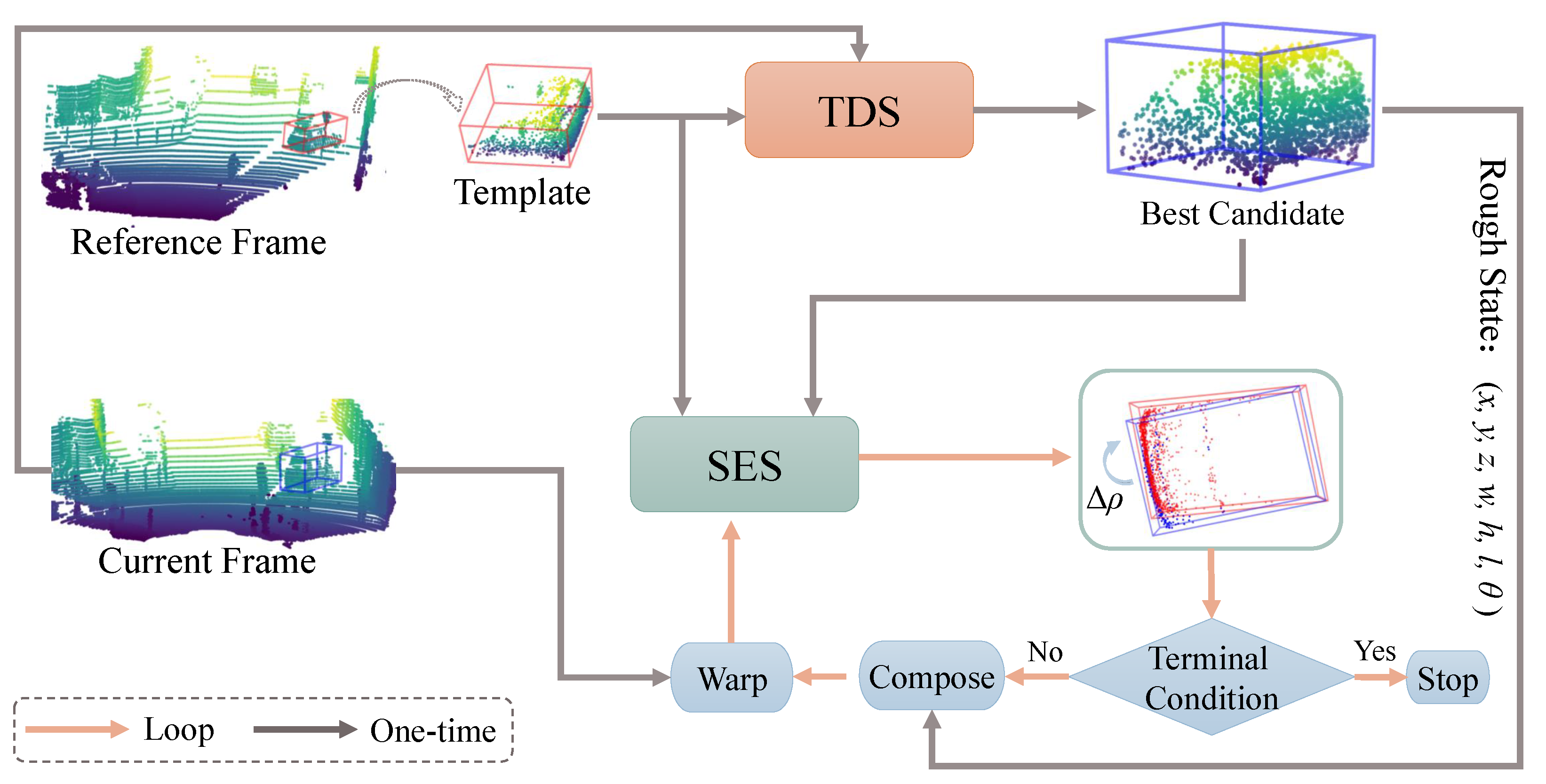
The proposed 3D point cloud tracking approach not only discriminates the target from distractors but also estimates the target state in a unified framework. Its pipeline is shown in Figure 1. Firstly, the template cropped from the reference frame and the current tracked frame are fed into the target discrimination subnetwork (TDS). It can select the best candidate in terms of the confidence score. Then, such selected candidate and the template are fed into the state estimation subnetwork (SES) to produce a incremental warp parameters . These parameters are applied to the rough state of the best candidate, leading to a new state. Next, the warped point cloud extracted by the new state is sent into the SES again, producing together with the template. This procedure is implemented iteratively until the terminal condition is satisfied. We use the same feature backbone but train the TDS and SES separately. In Section 3.2, we first present our SES in detail, which extends the LK algorithm for 2D tracking to 3D point clouds. In Section 3.3, the powerful TDS is introduced. Finally, in Section 3.4, we describe an online tracking strategy that illustrates how two components cooperate with each other.
3.2. State Estimation Subnetwork
Our state estimation subnetwork (SES) is designed to learn the incremental warp parameters between the template cropped from the first frame and candidate point clouds, so as to accommodate any motion variations. We took inspiration from DeepLK [19] and extended it to the 3D point cloud tracking task. To describe the state estimation subnetwork, we briefly revisit the inverse compositional (IC) LK algorithm [47] for 2D tracking.
The IC formulation is very ingenious and efficient because it avoids the repeated computation of the Jacobian on the warped source image. Given a template image T and a source image I, the essence of IC-LK is to solve the incremental warp parameters on T using sum-of-squared-error criterion. Therefore its objective function for one pixel can be formulated as follows:
where are currently known state parameters, is the number of increments the state parameters are to go through, are the pixel coordinates, and is the warp function. More concretely, if one considers the location shift and scale, i.e., , the warp function can be written as . Using the first-order Taylor expansion at the identity warp , the Equation (1) can be rewritten as
where is the identity mapping and represents the image gradients. Let the Jacobian . We hence can obtain by minimizing the above Equation (2); namely,
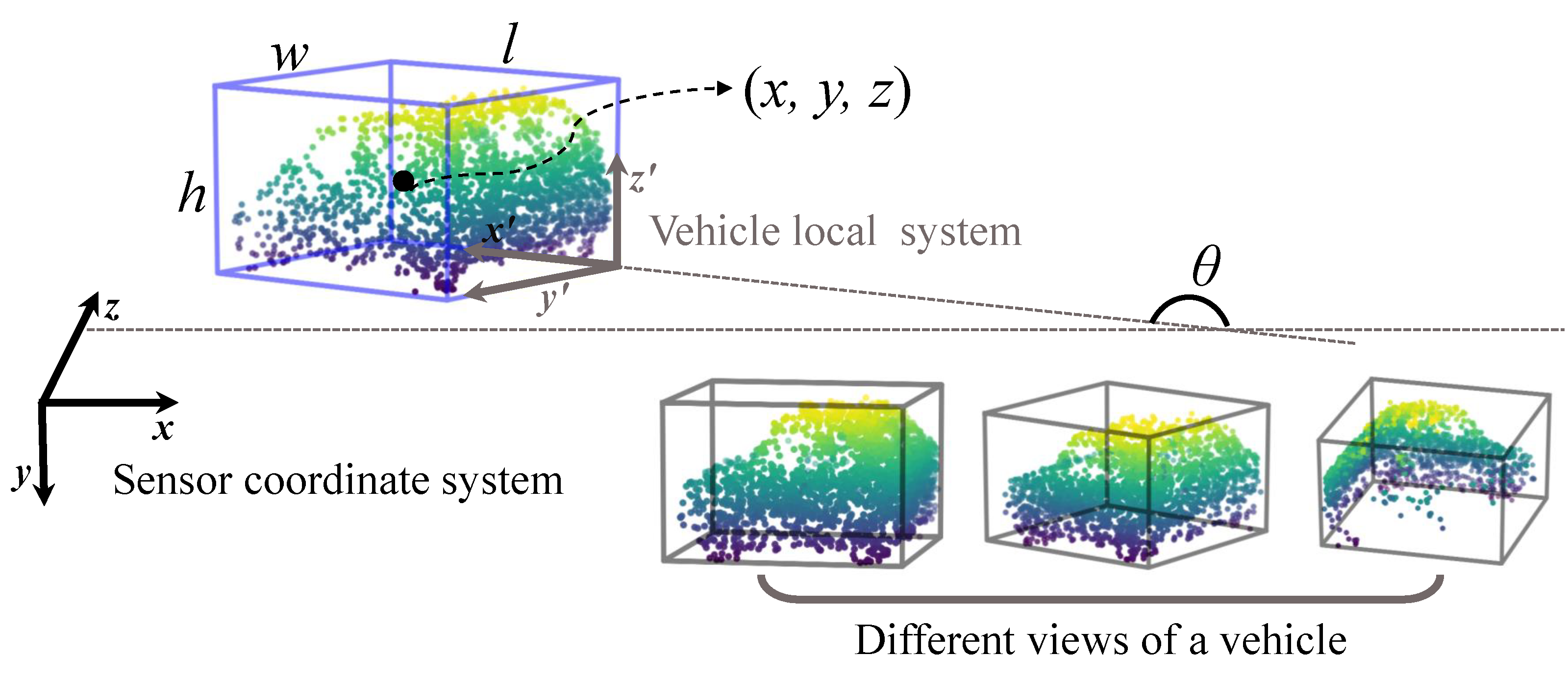
Compared with 2D visual tracking, 3D point cloud tracking has an unstructured data representation and high-dimensional search space for state parameters. Let denote the template point cloud. denotes the source point cloud in the tracked frames, which is extracted by a bounding box with inaccurate center and orientation. Note that we set the quantities of both and to N, and when their totals of points are less than N, we repeat sampling from existing points. In this work, we treat the deep network as a learnable “image” function. In light of this, the template point cloud and the source point cloud can obtain their descriptors using the network after transforming them into the canonical coordinate system. In addition, we regard the rigid transformation between and as the “warp” function. In this way, we can apply the philosophy of IC-LK to the 3D point cloud tracking problem. In practice, the 3D bounding box is usually utilized to represent the target state which can be parametrized by in the LiDAR system, as shown in Figure 2. Therein, is the target center coordinate, represents the target size, and is the rotation angle around the y-axis. Due to the target size remaining almost unchanged in 3D spatial space, it is sufficient to focus only on the state variations in the angle and x, y, and z axes. Consequently, the transformation G will be represented by four warping parameters . More concretely, it can be simplified as follows:
Now the state estimation problem in 3D tracking can be transformed to find satisfying , where is the warp operation on the homogeneous coordinate with . Being analogous to the aforementioned IC-LK in Equation (2), the objective of state estimation can be written as
Similar to the Equation (2), we could solve the incremental warp with the Jacobian matrix . Unfortunately, this Jacobian matrix cannot be calculated like the classical image manner. The core obstacle is that the gradients in x, y, and z cannot be calculated in the scattered point clouds due to the lack of connections among points or another regular convolution structure.
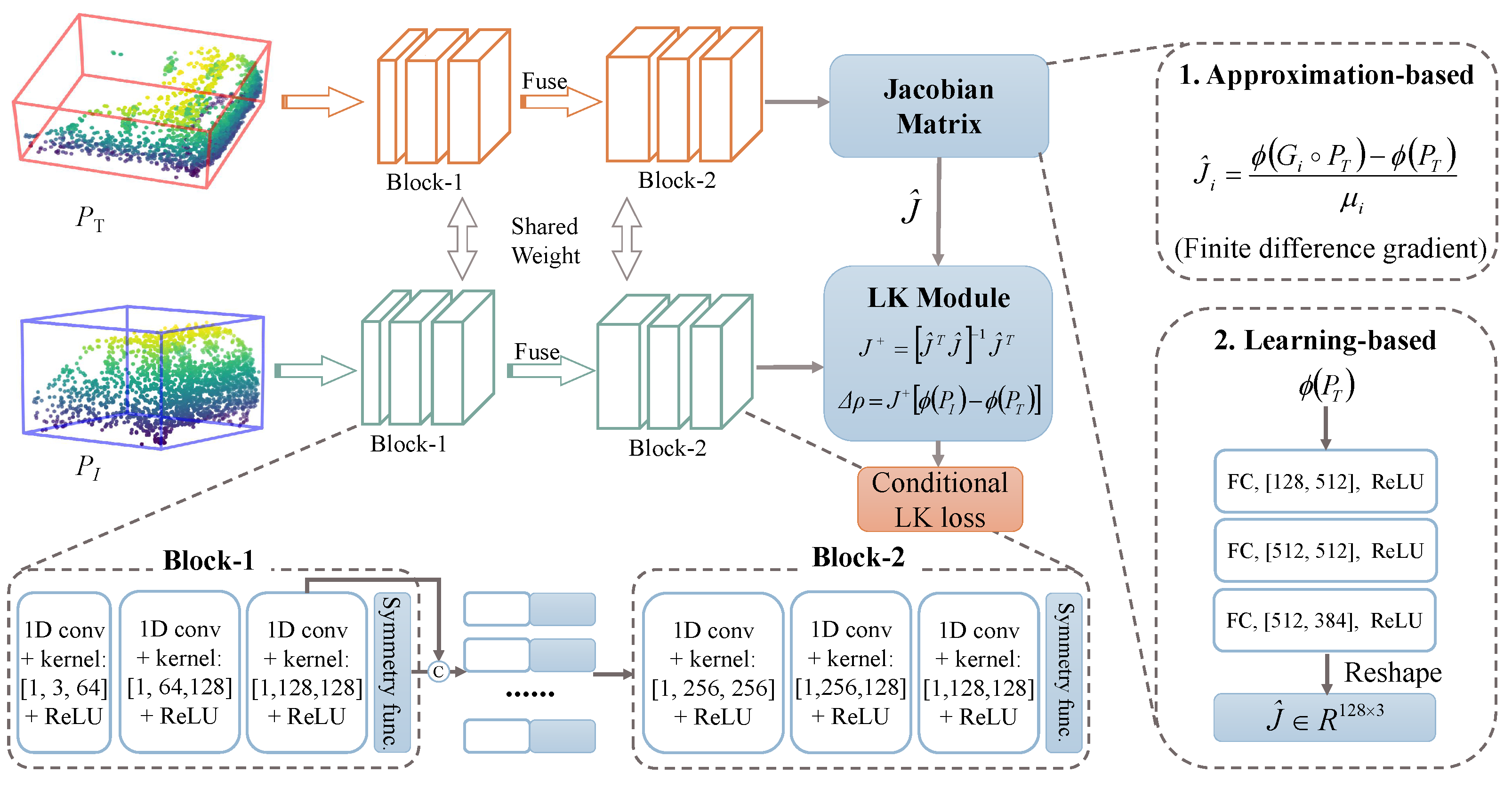
We introduce two solutions to circumvent this problem. One direct solution is to approximate the Jacobian matrix through a finite difference gradient [48]. Each column of the Jacobian matrix can be computed as
where are infinitesimal perturbations of the warp parameters , and is a transformation involving only one of the warp parameters. (In other words, only the i-th warp parameter has a non-zero value . Please refer to Appendix A for details).
On the other hand, we treat the construction of as a non-linear function with respect to . We hence propose an alternative: to learn the Jacobian matrix using a multi-layer perceptron, which consists of three fully-connected layers and ReLU activation functions (Figure 3). In Section 4.4, we report the comparison experiments.
Based on the above extension, we can analogously solve the incremental warp of the 3D point cloud in terms of Equation (3) as follows:
where is a Moore–Penrose inverse of . Afterwards, the source point cloud cropped from the coming frame can adjust its state by the following formula
where is the inverse compositional function and is the state representation of the source point cloud .
Network Architecture.Figure 3 summarizes the architecture of the state estimation subnetwork. Owing to the inherent complexity of the state estimation, it is non-trivial to train a powerful estimator on the fly under the sole supervision of the first point cloud scenario. We hence train the SES offline to learn general properties for predicting the incremental warp. It is natural that we opt to adopt a Siamese architecture for producing the incremental warp parameters between the template and candidate. In particular, our network contains two branches sharing the same feature backbone, each of which consists of two blocks. As shown in Figure 3, Block-1 first generates the global descriptor. Then Block-2 consumes the aggregation of the global descriptor and the point-wise features to generate the final K-dimensional descriptor, based on which the Jacobian matrix can be calculated. Finally, the LK module jointly considers , , and to predict . It is notable that this module theoretically provides the fusion strategy, namely, , between two features produced by the Siamese network. Moreover, we adopt the conditional LK loss [19] to train this subnetwork in an end-to-end manner. It is formulated as
where is the ground-truth warp parameter, is the smooth function [49], and M is the number of paired point clouds in a mini-batch. This loss can propagate back to update the network when the derivative of the batch inverse matrix is implemented.
3.3. Target Discrimination Subnetwork
In the 3D search space, how to efficiently determine the presence of the target is very critical for an agent to conduct state estimation. In this section, considering that the SES lacks discrimination ability, we present the design of a target discrimination subnetwork (TDS) to realize a strong alliance with the SES. It aims to distinguish the best candidate from distractors, thereby providing a rough target state. We leverage the matching function based method [2] to track the target. Generally, its model can be written as
where is the confidence score function, is the feature extractor, and g is a similarity metric. Under this framework, the candidate with the highest score is selected as the target.
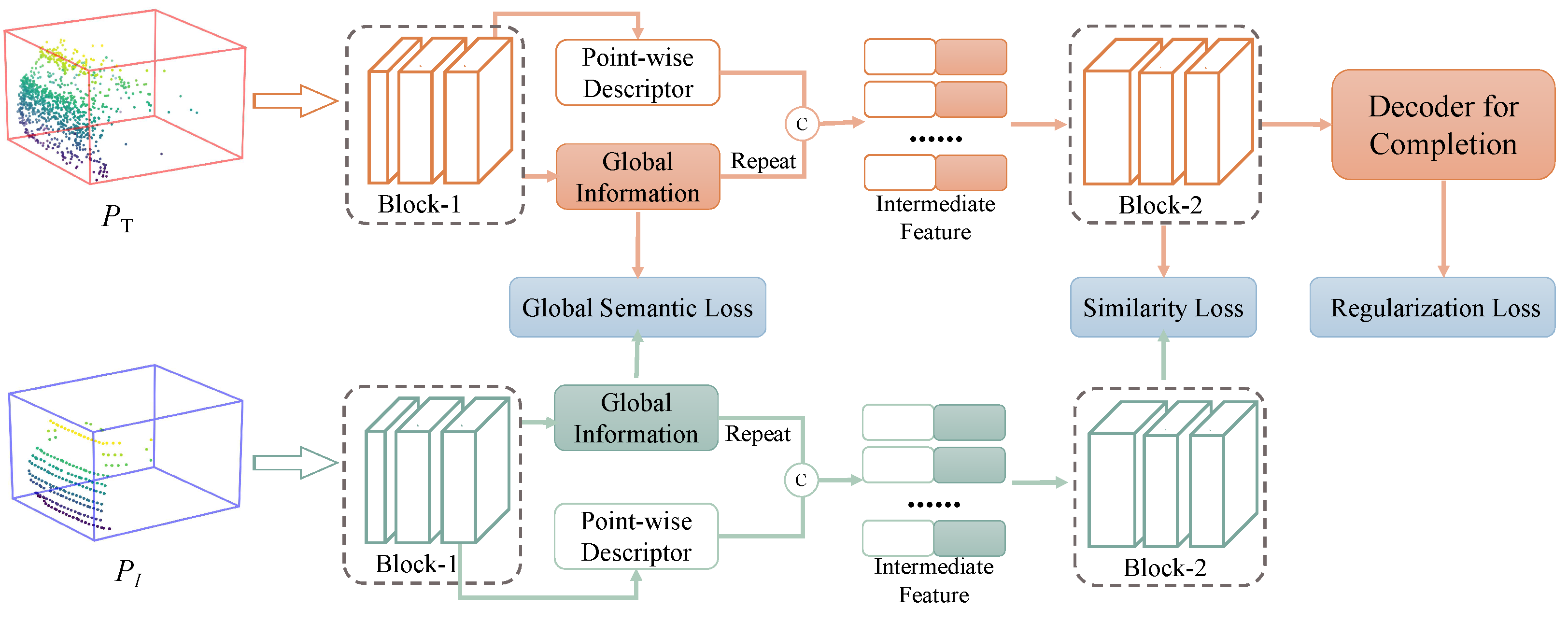
In this work, to equip the model with global semantic information, we incorporate the intermediate features generated by the first block to point-wise features, and then pass them to the second block, as shown in Figure 4. Consequently, our TDS could project 3D partial shapes into a more discriminatory latent space, which allows an agent to distinguish the target more accurately from distractors.
Network Architecture. We trained the TDS offline from scratch with an annotated KITTI dataset. Based on the Siamese network, the TDS takes paired point clouds as inputs and directly produces their similarity scores. Specifically, its feature extractor also consists of two blocks the same as in the SES. As can be seen in Figure 4, Block-1 generates the global descriptor, and Block-2 utilizes the aggregation of the global point-wise features to generate the more discriminative descriptor. As for the similarity metric g, we conservatively utilize hand-crafted cosine function. Finally, the similarity loss, global semantic loss, and regularization completion loss are combined in order to train this subnetwork; i.e.,
where is mean square error loss, s is the ground-truth score, is the balance factor, and is the completion loss for regularization [2], where represents each template point cloud predicted via shape completion network [2].
3.4. Online Tracking
Once trained offline, the two subnetworks can be combined for online tracking. We denote our whole framework SETD. For one scenario (frame) , , where Q is the total number of frames, we first sampled a collection of candidates in terms of Kalman filter as SiamTrack3D does, and then passed them into the TDS, which provided the rough state representation of the optimal candidate. Afterwards, it was adjusted iteratively by the SES until the termination condition was satisfied, and the best state was thus determined. Finally, the template point cloud was updated by appending the selected candidate to itself. Algorithm 1 shows the whole process in detail.
| Algorithm 1: SETD online tracking. |
 |
4. Experiments
KITTI [50] is a prevalent dataset of outdoor LiDAR point clouds. Its training set of contains 21 scenes (over 27,000 frames), and each frame has about 1.2 million points. For a fair comparison, we followed [2] to divide this dataset into a training set (scene 0–16), a validation set (scene 17–18), and a testing set (scene 19–20). In addition, to validate the effectiveness of different trackers, we also evaluated them on another large-scale point cloud dataset—PandaSet [51]. It covers complex driving scenarios, including lighting conditions at day time and night, steep hills, and dense traffic. In this dataset, more than 25 scenes were collected for testing, and the tracked instances are split into three levels (easy, middle, and hard) according to the LiDAR range.
4.1. Evaluation Metrics
To evaluate the tracking results, we adopted one-pass evaluation (OPE) [21] based on the location error and the overlap. The overlap represents the intersection-over-union (IoU) between the predicted bounding box and the corresponding ground-truth bounding box , i.e., . The location error measures the Euclidean distance between the centers of and . In this paper, the success and precision metrics are utilized as evaluation metrics. Specifically, the success metric is defined as the area-under-curve (AUC) where the x-axis denotes the overlap threshold ranging from 0 to 1 and the y-axis refers to the ratio above the threshold. The precision metric is defined as the AUC where the x-axis represents the location error threshold ranging from 0 to 2 meters and the y-axis is the ratio below this threshold.
4.2. Implementation Details
Training. We conducted experiments with PyTorch and Python 3.7 on a PC equipped with a GTX 2080Ti, 32 GB RAM, and 4.00 GHz Intel Core i7-4790K CPU. When training our SES, we first sampled a pair of target shapes (template and source point clouds) from the same sequence. Additionally, these two point clouds were transformed into a canonical coordinate system according to the respective bounding box. Assuming that the target motion obeyed the Gaussian distribution, we randomly produced the warp parameters and applied them to the source point clouds for the supervised learning. In practice, only when the IoU between the warped bounding box and its corresponding ground truth is larger than 0.1 can this paired data be fed into the SES. The mean of Gaussian distribution was set to zero, and the covariance was a diagonal matrix . The dimension K of shape descriptor generated by was set to 128. The network was trained from scratch using the Adam optimizer with the batch size of 32 and the initial learning rate of .
Regarding our TDS, the input data were the paired point clouds transformed into a canonical coordinate system. The outputs were similarity scores. The ground-truth score is the soft distance obtained by the Gaussian function. The output dimensions K of were set to 128. Our proposed loss (Equation (11)) was utilized to train it from scratch using an Adam optimizer. The batch size and initial learning rate were set to 32 and , respectively. As for , we reported its performance using several metrics in Section 4.4. The learning rates of both subnetworks were reduced via multiplying by a ratio of 0.1 when the loss of the validation set reached a plateau, and the maximum number of epochs was set to 40.
Testing. During the online testing phase, the tracked vehicle instance was usually specified in the first frame. When dealing with a coming frame, we exhaustively drew a set of 3D candidate boxes over the search space [2]. The number of was set to 125. The number of iterations was set to 2, and the termination parameter was set to . Besides, for each frame, our SETD tracker only took about 120 ms of GPU time (50 ms for the TDS and 70 ms for the SES) to determine the final state. We did not take into account the time cost of the generation and normalization of the template and candidates, which was 300 ms of CPU time, approximately.
4.3. Performance Comparison
We first compare the proposed SETD with the baseline in relation to several attributes, such as dynamics and occlusion. Then, we evaluate the tracking performances of recent related trackers on large-scale datasets.
4.3.1. Comparison with Baseline
SiamTrack3D [2] was the first method made to deal with this special task using the Siamese network and gives some referential insights via adequate ablation studies. It is a strong baseline for state-of-the-art tracking performance. We first show visualization comparison results for different attributes in Figure 5, Figure 6 and Figure 7, and then report quantitative comparison results in Table 1.
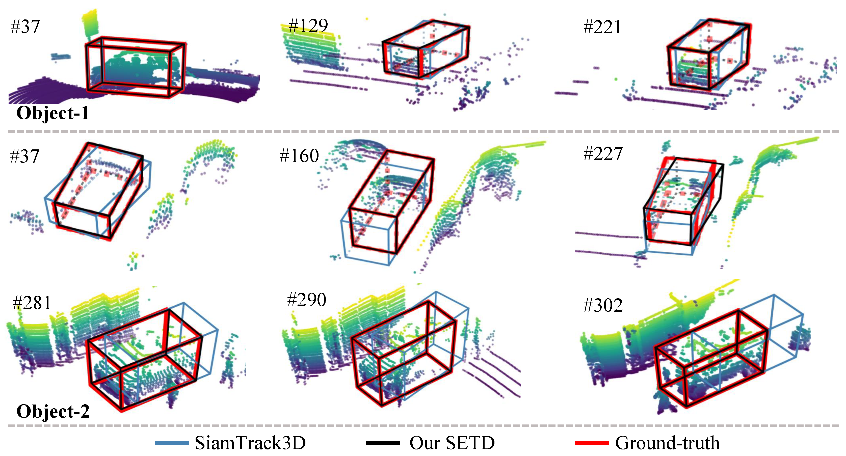
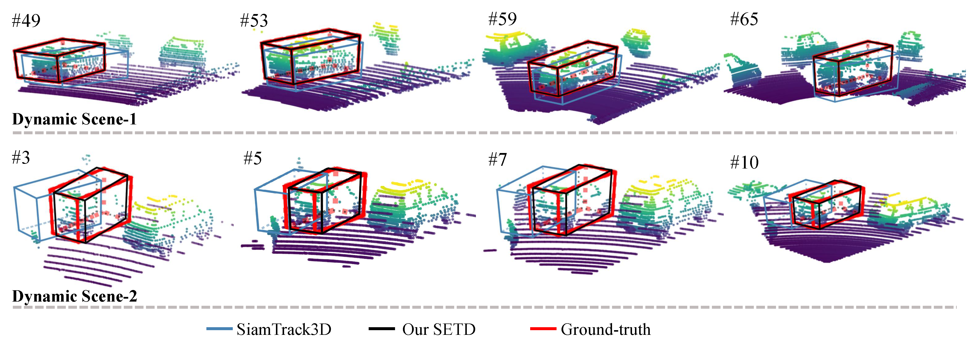
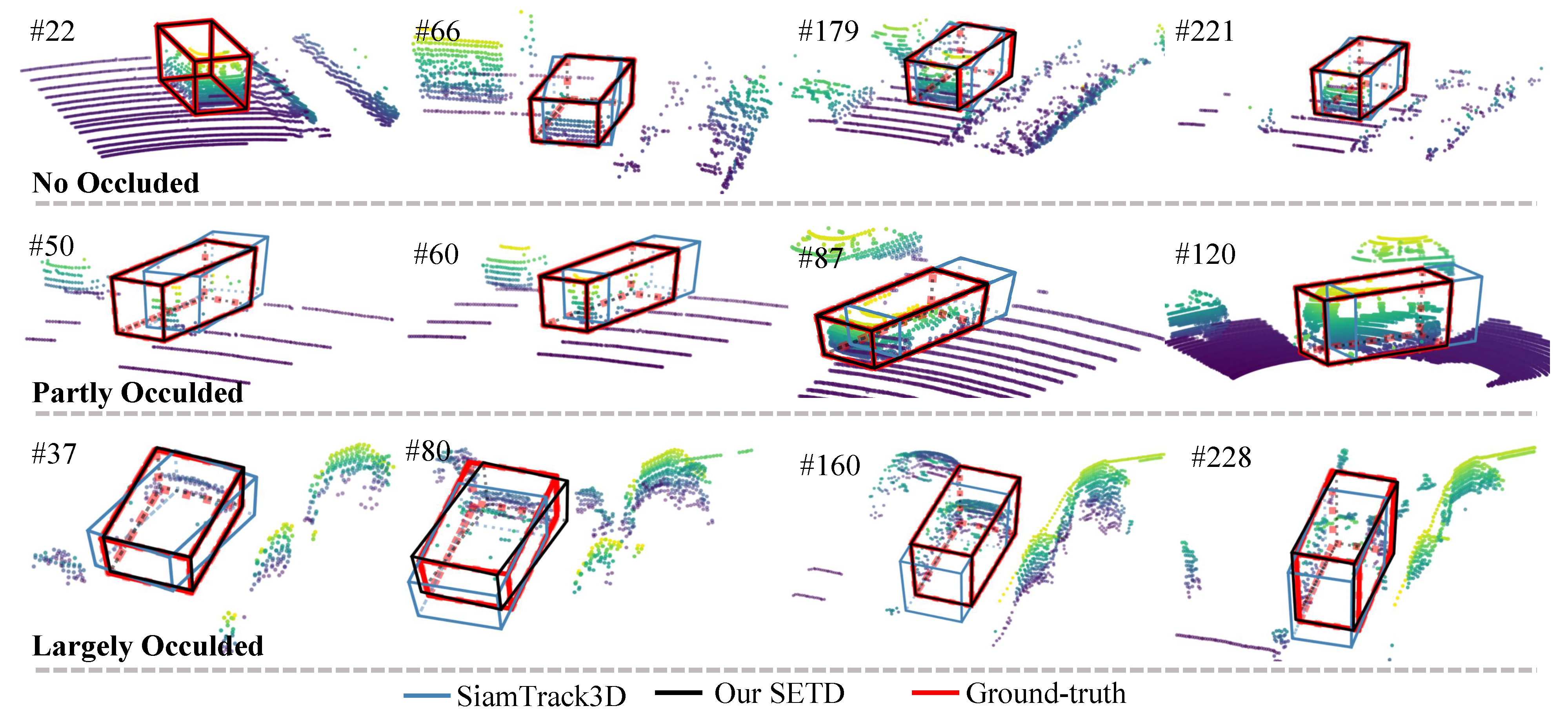
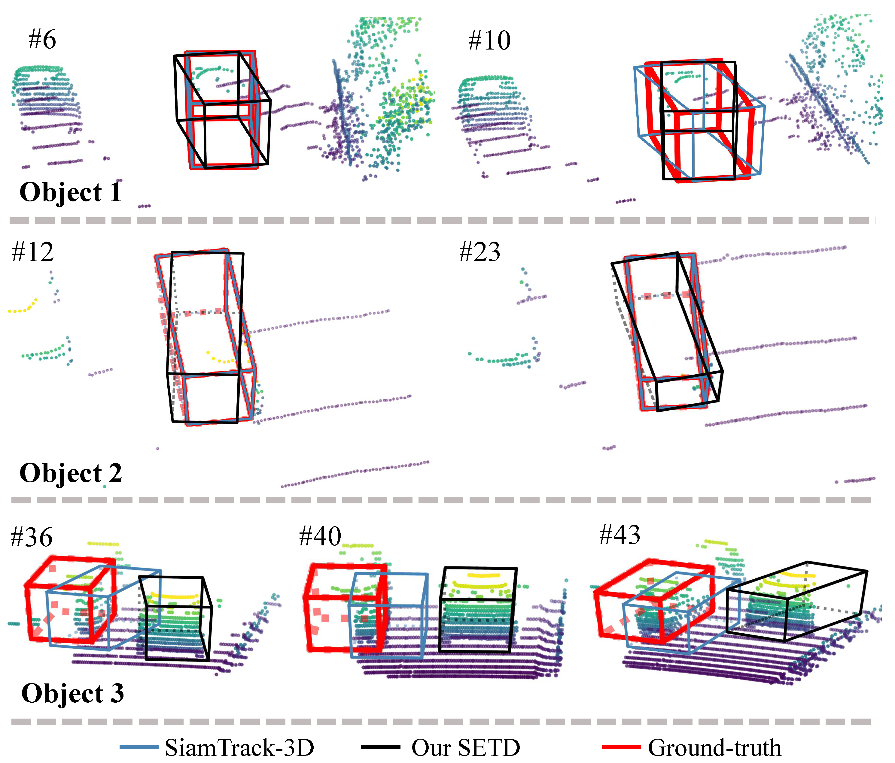
Figure 5 shows a visualization of density variation. As can be seen, “Object-1” changed from dense to sparse, and “Object-2” varied from sparse to dense. For all these scenes, our method tracked the target accurately, whereas SiamTrack3D exhibited skewing. Figure 6 presents some tracking results for dynamic scenes. Generally, the scene is treated as dynamic when the center distance between consecutive frames is larger than [2]. As shown in Figure 6, our method performed better than SiamTrack3D when the target moved quickly, which is attributed to the seamless integration of target discrimination and state estimation. In particular, even though the target was partly occluded and moving at high speed in the scenario presented in the second row, SETD obtained satisfying results, whereas SiamTrack3D produced greatly varying results. Figure 7 plots the tracking results from when the target suffered from different degrees of occlusion. As can be seen, whether the target was visible, partly occluded, or largely occluded, our SETD performed better than SiamTrack3D.
In addition, we quantitatively compared their performances according to four conditions: visible, occluded, dynamic, and static. The success and precision metrics for said attributes are shown in Table 1. Overall, the proposed SETD fully outperformed SiamTrack3D. Specifically, compared with SiamTrack3D, SETD not only significantly improved detection by 16.45%/13.61% (success/precision) in visible scenes, but also 11.31%/14.43% in occluded scenes. Meanwhile, as shown in the last two rows of Table 1, SETD also achieved great improvements of 7.68%/7.92% when detecting dynamic scenes, and 16.54%/16.73% when detecting static scenes. These significant improvements on four types of scenes thoroughly and powerfully demonstrate the effectiveness of learning incremental warp for accurate 3D point cloud tracking.
4.3.2. Comparison with Recent Methods
Apart from SiamTrack3D, we compared with other methods—AVODTrack [14], P2B [16], SiamTrack3D-RPN [52], and ICP&TDS—on the testing set. AVODTrack is a tracking-by-detection method which evolved from an advanced 3D detector, AVOD [14], by equipping it with an online association algorithm. To be more precise, it consumes point cloud BEVs and RGB images to generate a 3D detection box for every frame; then the final box is the one that has the highest IoU with the previous bounding box. P2B is a new, advanced method which integrates the target feature augmentation module into deep Hough voting [17]. SiamTrack3D-RPN evolved from SiamTrack3D by jointly learning on 2D BEV images and 3D point clouds. Furthermore, to estimate the state of moving vehicles, one may intend to obtain the motion transformation using the iterative closest point (ICP) [53], and then apply this transformation to previous bounding box. In this work, we first leveraged the proposed TDS to obtain a candidate point cloud and then run the ICP algorithm between the template and this candidate in a canonical coordinate system. This method is called ICP&TDS. In SiamTrack3D, as in the Kalman filter, the ground truth of the tracked frame is also utilized to approximate dense sampling for further testing of a tracker’s discrimination ability. It applies grid search centered at the tracked ground truth. We also considered this sampling strategy for comprehensive evaluation. Note that a method with the suffix “Dense” means that it adopts this dense sampling.
Table 2 summarizes the above methods’ performances on KITTI. In addition to conducting OPE of the 3D bounding box, we also present the results of the 2D BEV box, which was obtained by projecting the 3D box onto a rectangle from a bird’s-eye view. As shown in this table, SETD-Dense is superior to all other methods, given its high success and precision metrics. Specifically, the success and precision metrics of our SETD constituted 13.68% and 13.48% improvements compared with SiamTrack3D, and our SETD-Dense provided 5.12% and 6.77% improvements over SiamTrack3D-Dense. This demonstrates the validity of bridging the gap between state estimation and target discrimination. ICP&TDS and ICP&TDS-Dense obtained poor performances in these specific outdoor scenes. We deem that ICP lacks strength for partial scanned point clouds. This also proves that the proposed SES plays a critical role in the point cloud tracking task. In addition, even when using multiple modalities of RGB images and LiDAR point clouds, AVODTrack was inferior to the dense sampling models (SiamTrack3D-Dense and SETD-Dense) by large margins. P2B obtained better performances than SiamTrack3D and SETD, because P2B uses a learning procedure based on deep Hough voting to generate high quality candidates, whereas SiamTrack3D and SETD only use traditional Kalman filter sampling. Hence, better candidate generation is important for the following tracking process, and we recon that integrating a learning-based candidate generation strategy into SiamTrack3D and SETD will facilitate improving their accuracy.
Table 3 reports the tracking results on PandaSet. We compare the proposed method with two advanced open-source trackers: P2B and SiamTrack3D. Their performances were obtained by running their official code on our PC. As shown in the Table 3, our SETD performed considerably better than P2B in all easy, middle, and hard sets, especially in obtaining the success/precision improvements of 6.77/9.34% with the middle set. When compared with SiamTrack3D, SETD also outperformed it by a large margin on easy and middle sets. Nevertheless, on the hard set, SETD was inferior to SiamTrack3D. The reasons were that: (1) there exist some extremely sparse objects in the hard set, which makes the SES product a worse warp parameter, (2) SiamTrack3D has a better prior because it is first trained on ShapeNet and then fine-tuned on KITTI, whereas SETD is trained only from scratch.
4.4. Ablation Studies
We carried out five self-contrast experiments to demonstrate the necessity of each part.
SES and TDS. In order to prove the effectiveness of the combination of the state estimation and the target discrimination, we examined the tracking performance only using TDS or SES. TDS-only tracks the target merely via the target discrimination subnetwork, which selects a candidate bounding box with the highest confidence score. Based on the state estimation subnetwork, SES-only directly rectifies the estimated bounding box of the previous frame for tracking the target. Our SETD properly combines these two components to make up for their performance gap.
The results are shown in Table 4. According to the success metric, our SETD achieved 10.41% and 11.28% improvements in comparison with SES-only and TDS-only, respectively. As for the precision metric, SETD (69.65%) also significantly surpassed both SES-only (49.70%) and TDS-only (60.19%). These improvements of SETD highlight the importance of combining these two components. In addition, we observed that SES-only performed worse than TDS-only according to the success and precision metrics. The main reason lies in that (1) TDS-only selects the best one of many candidates generated by the Kalman filter, but SES-only directly uses the previous result while lacking discrimination; (2) the previous result used by SES often drifts due to self-occlusion and density variations, leading to far-fetched warp parameters. This also proves our observation mentioned in Section 3.3: that determining the presence of the target is crucial for an agent to conduct state estimation.
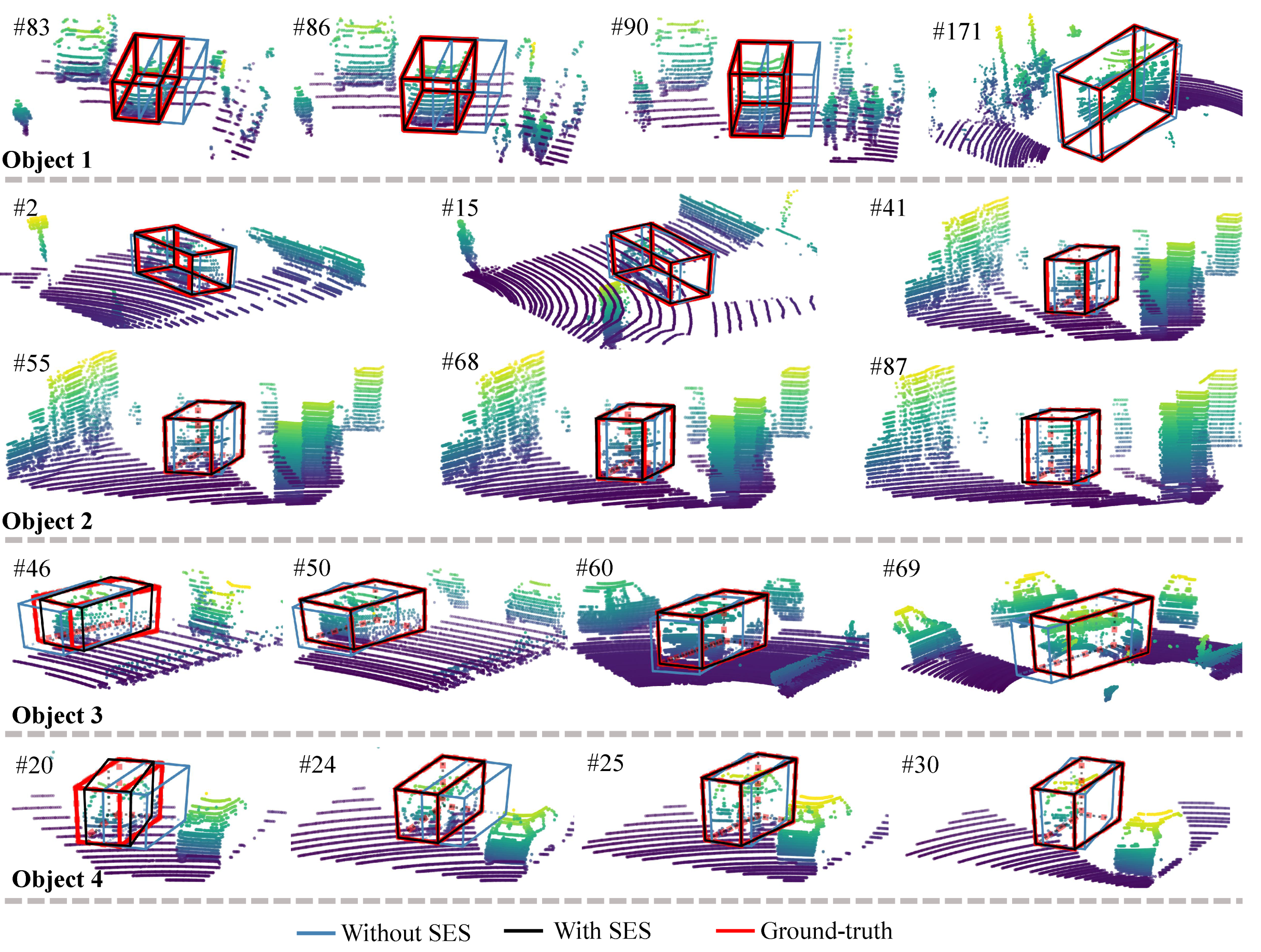
Moreover, Figure 8 presents some tracking results obtained without or with our state estimation subnetwork. As can be seen when going through the state estimation subnetwork, some inaccurate results (blue boxes), which were predicted solely via a target discrimination subnetwork, can be adjusted towards the corresponding ground truth.
Iteration or not. We also investigated the effect of iteratively adjusting the target state. Specifically, we designed a variant model named Iter-non, which does not apply the iterative online tracking strategy (Algorithm 1). In other words, it directly uses the first prediction of the SES as the final state increment. As shown in Table 4, Iter-non obtained a 44.67% success ratio and a 59.13% precision ratio on the KITTI tracking dataset. Compared with SETD (53.77%/69.65%), Iter-non fell short by 9% in success and precision metrics, which proves the effectiveness of our iterative online tracking strategy. In fact, the iteration process is an explicit cascaded regression that is more effective and verifiable for tasks solved in continuous solution spaces [19,48,54].
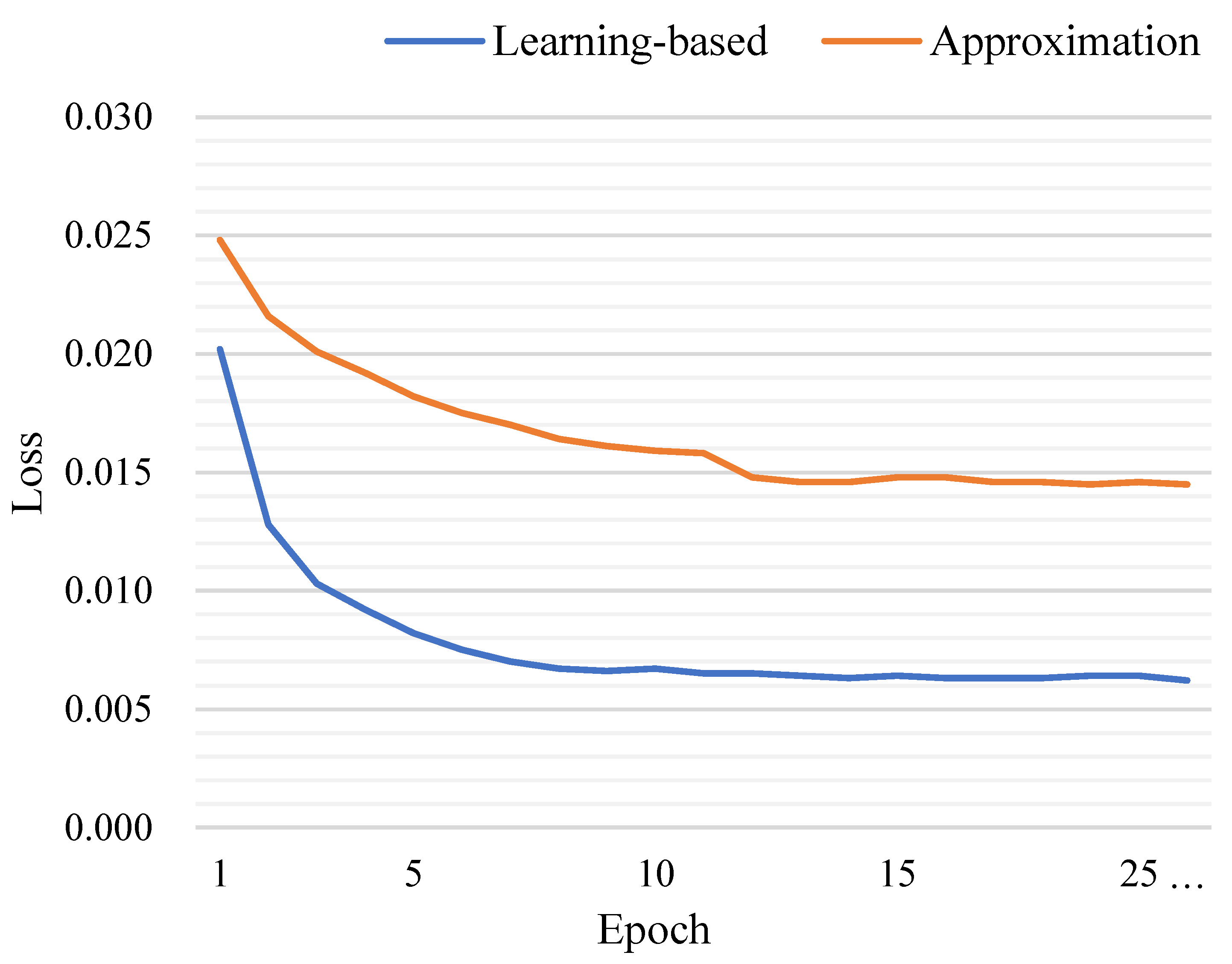
Jacobian Approximation or Learning. Two solutions have been provided to tackle the Jacobi matrix issue that occurred in the SES. We can approximate it via finite difference gradient or learn it using a multi-layer perceptron. To comprehensively compare these two solutions, we plotted their loss curves during the training phase in addition to reporting the success and precision metrics on the testing set. As shown in Figure 9, the learning-based solution had a far lower cost and flatter trend than the approximation-based one. Moreover, the last row of Table 5 shows the approximation-based solution achieved success/precision of 49.93%/67.15%; the learning-based solution reached 53.77%/69.65%. The reason may be that a teachable Jacobian module could be coupled with the shape descriptor , whereas the finite difference gradient defined by a hand-crafted formula is a hard constraint. Please refer to Appendix B for more details.
Descriptor Using Block-1 or Block-2. A cascaded network architecture is proposed for the 3D point cloud tracking problem. We explored the impact of using descriptors generated by different feature blocks when extending the traditional LK algorithm to the 3D point cloud tracking task. Each column of Table 5 shows that the descriptor from Block-2 is superior that from Block-1. This benefits from the novelty that we incorporate the global semantic information into point-wise features.
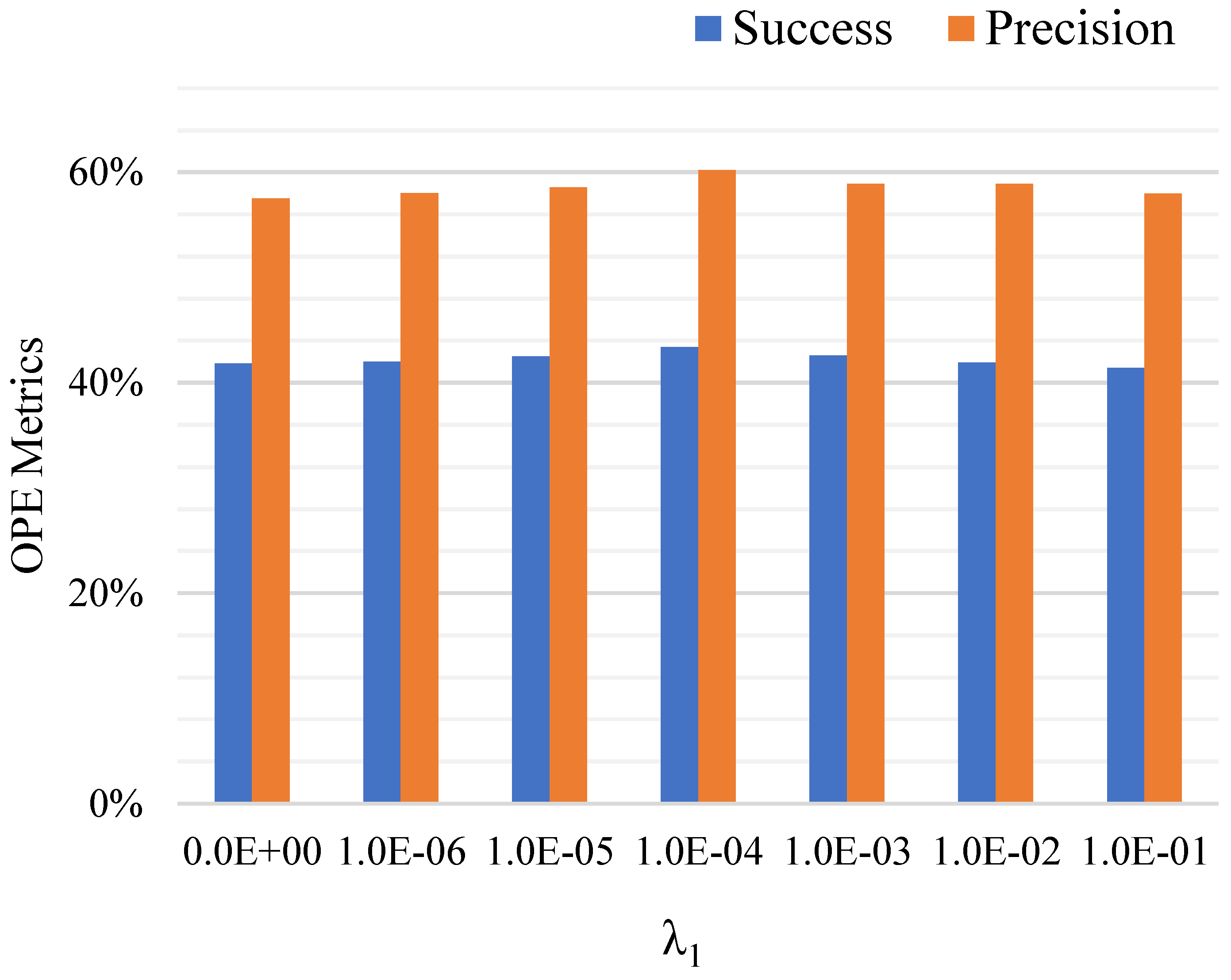
Key Parameter Analysis. In Section 3.3, in order to robustly determine the presence of the target in a point cloud scenario, we proposed a new loss that combines similarity loss, global semantic loss, and regularization completion loss. Therein, the parameter in Equation (11) plays a key role in the global information trade-off. In Figure 10, we compared different values of . As we can see, it obtained the best performance in success and precision metrics when .
4.5. Failure Cases
Figure 11 shows some failure cases of our proposed model. In this figure, “Object 1” (the first row) and “Object 2” (the second row) could not be tracked accurately by our SETD (black). The reason is that the extremely spare points could not extract an explicit pattern to discriminate target or estimate state. “Object 3” (the last row) drifted to similar distractors surrounding the target. This is because the previous bounding box, when applied to the current frame, covered similar adjacent objects due to its very fast movement.
5. Conclusions and Future Work
This paper presents a 3D point cloud tracking framework bridging the gap between state estimation and target discrimination subnetworks. Particularly, the traditional LK algorithm has been creatively extended to the case of 3D tracking for accurate state estimation. Meanwhile, a new loss method was proposed in the hopes of providing more powerful target discrimination. Experiments on the KITTI and PandaSet datasets have shown our method significantly outperforms others. Last but not least, the ablation studies fully demonstrated the effectiveness of each part and gave some key analyses of the descriptor, iteration strategy, and Jacobian matrix calculation.
SiamTrack3D [2] is the first point cloud tracker based on the Siamese network. This method starts with state estimation and target discrimination (inspired by 2D tracker [18,19]), and extends them to 3D point cloud tracking. Although achieving promising performance, it has huge room for improvement. For example, both SiamTrack3D and SETD are struggling with the proposal extraction issue. To be specific, they obtain proposals via Kalman filter or a dense sampling strategy. In light of this, in the future, it will be very important to explore an efficient proposal extraction algorithm. Despite the recent literature [52] providing better proposals via BEV, the joint learning on 2D BEV and 3D point cloud Siamese networks even drops the final discrimination ability. Besides, a new feature backbone [41,55] is also worth studying instead of using pointNet, which is used alone in SiamTrack3D. Last but not least, it will be important to study an end-to-end network, including the flow embedding layer [56], proposal generation, similarity metric, and state refinement.
Author Contributions
Conceptualization, S.T. and X.L.; methodology, S.T. and X.L.; validation, S.T.; formal analysis, S.T., M.L. and X.L.; investigation, S.T. and Y.B.; writing—original draft preparation, S.T. and M.L.; writing—review and editing, M.L. and J.G.; visualization, S.T. and Y.B.; supervision, X.L. and B.Y.; project administration, S.T. All authors have read and agreed to the published version of the manuscript.
Funding
This work was funded by the National Natural Science Foundation of China (grant number 61976040 and U1811463) and the National Key Research and Development Program of China (grant number 2020YFB1708902).
Institutional Review Board Statement
Not applicable.
Informed Consent Statement
Not applicable.
Data Availability Statement
The KITTI tracking dataset is available at http://www.cvlibs.net/download.php?file=data_tracking_velodyne.zip; accessed on 24 June 2021. The PandaSet dataset is available at https://scale.com/resources/download/pandaset; accessed on 24 June 2021. For the reported results, one can obtain it by request to corresponding author.
Conflicts of Interest
The authors declare no conflict of interest.
Appendix A. Details of Approximation-Based Solution
After extending the LK algoritm [19] designed for 2D visual tracking to 3D point cloud tracking task, we have the following objective
As the warp parameters and , the Jacobian matrix in the Equation (A1) belongs to . The formula of the finite difference gradient [48] is as follows:
We use infinitesimal perturbations to approximate each column of . Therein, , corresponds to the transformation that is obtained by only perturbing the i-th warp parameter, which can be formulated as
When training the SES by approximation-based solution, we set the infinitesimal perturbations to 0.1.
Appendix B. Analysis of the Jacobian Module
Our loss is defined as follows:
To enable the state estimation network to be trained in an end-to-end way, the differentiation of the Moore-Penrose inverse in Equation (A4) needs to be derived as [19] did. Concretely, the partial derivative of smooth function over the feature component can be written as
where is one-hot vector and is the derivative of the smooth loss. Besides, the partial derivative of smooth function over the is
Therein, the key step is to obtain the differentiation of . By the chain rule, it can be written as
where
According to the above equation, the derivative of a batch inverse matrix can be implemented in PyTorch such that the SES network can be trained in an end-to-end manner.
In this work, we present two solutions for calculating the Jacobian in our paper. Here we give their back-propagation formulae to deeply compare them with each other. When using multi-layer perceptron (learning-based) to calculate the Jacobian, the elements of are related to each component of . We hence have
where is adaptively updated.
When using finite difference gradient (approximition-based), we have
where
and
As can be seen from the above formulae, in the finite difference is fixed while the learning function is updated adaptively in the multi-layer perception. Thus, the learning-based solution may be more easily coupled with the feature extractor than the approximation-based one.
References
- Ma, Y.; Anderson, J.; Crouch, S.; Shan, J. Moving Object Detection and Tracking with Doppler LiDAR. Remote Sens. 2019, 11, 1154. [Google Scholar] [CrossRef] [Green Version]
- Giancola, S.; Zarzar, J.; Ghanem, B. Leveraging Shape Completion for 3D Siamese Tracking; CVPR: Salt Lake City, UT, USA, 2019; pp. 1359–1368. [Google Scholar]
- Comport, A.I.; Marchand, E.; Chaumette, F. Robust Model-Based Tracking for Robot Vision; IROS: Prague, Czech Republic, 2004; pp. 692–697. [Google Scholar]
- Wang, M.; Su, D.; Shi, L.; Liu, Y.; Miró, J.V. Real-time 3D Human Tracking for Mobile Robots with Multisensors; ICRA: Philadelphia, PA, USA, 2017; pp. 5081–5087. [Google Scholar]
- Luo, W.; Yang, B.; Urtasun, R. Fast and Furious: Real Time End-to-End 3D Detection, Tracking and Motion Forecasting with a Single Convolutional Net; CVPR: Salt Lake City, UT, USA, 2018; pp. 3569–3577. [Google Scholar]
- Schindler, K.; Ess, A.; Leibe, B.; Gool, L.V. Automatic detection and tracking of pedestrians from a moving stereo rig. ISPRS J. Photogramm. Remote Sens. 2010, 65, 523–537. [Google Scholar] [CrossRef]
- Nam, H.; Han, B. Learning Multi-Domain Convolutional Neural Networks for Visual Tracking; CVPR: Salt Lake City, UT, USA, 2016; pp. 4293–4302. [Google Scholar]
- Henriques, J.F.; Caseiro, R.; Martins, P.; Batista, J. High-Speed Tracking with Kernelized Correlation Filters. IEEE Trans. Pattern Anal. Mach. Intell. 2015, 37, 583–596. [Google Scholar] [CrossRef] [PubMed] [Green Version]
- Bertinetto, L.; Valmadre, J.; Golodetz, S.; Miksik, O.; Torr, P.H.S. Staple: Complementary Learners for Real-Time Tracking; CVPR: Salt Lake City, UT, USA, 2016; pp. 1401–1409. [Google Scholar]
- Liu, Y.; Jing, X.Y.; Nie, J.; Gao, H.; Liu, J.; Jiang, G.P. Context-Aware Three-Dimensional Mean-Shift With Occlusion Handling for Robust Object Tracking in RGB-D Videos. IEEE Trans. Multimed. 2019, 21, 664–676. [Google Scholar] [CrossRef]
- Kart, U.; Kamarainen, J.K.; Matas, J. How to Make an RGBD Tracker? ECCV: Munich, Germany, 2018; pp. 148–161. [Google Scholar]
- Bibi, A.; Zhang, T.; Ghanem, B. 3D Part-Based Sparse Tracker with Automatic Synchronization and Registration; CVPR: Salt Lake City, UT, USA, 2016; pp. 1439–1448. [Google Scholar]
- Luber, M.; Spinello, L.; Arras, K.O. People Tracking in RGB-D Data With On-Line Boosted Target Models; IROS: Prague, Czech Republic, 2011; pp. 3844–3849. [Google Scholar]
- Ku, J.; Mozifian, M.; Lee, J.; Harakeh, A.; Waslander, S.L. Joint 3D Proposal Generation and Object Detection from View; ICRA: Philadelphia, PA, USA, 2018; pp. 5750–5757. [Google Scholar]
- Yang, B.; Luo, W.; Urtasun, R. PIXOR: Real-Time 3D Object Detection from Point Clouds; CVPR: Salt Lake City, UT, USA, 2018; pp. 7652–7660. [Google Scholar]
- Qi, H.; Feng, C.; Cao, Z.; Zhao, F.; Xiao, Y. P2B: Point-to-Box Network for 3D Object Tracking in Point Clouds; CVPR: Salt Lake City, UT, USA, 2020; pp. 6328–6337. [Google Scholar]
- Qi, C.R.; Litany, O.; He, K.; Guibas, L.J. Deep Hough Voting for 3D Object Detection in Point Clouds; ICCV: Seoul, Korea, 2019; pp. 9276–9285. [Google Scholar]
- Danelljan, M.; Bhat, G.; Khan, F.S.; Felsberg, M. ATOM: Accurate Tracking by Overlap Maximization; CVPR: Salt Lake City, UT, USA, 2019; pp. 4655–4664. [Google Scholar]
- Wang, C.; Galoogahi, H.K.; Lin, C.H.; Lucey, S. Deep-LK for Efficient Adaptive Object Tracking; ICRA: Brisbane, Australia, 2018; pp. 626–634. [Google Scholar]
- Danelljan, M.; Bhat, G.; Khan, F.S.; Felsberg, M. ECO: Efficient Convolution Operators for Tracking; CVPR: Salt Lake City, UT, USA, 2017; pp. 6931–6939. [Google Scholar]
- Wu, Y.; Lim, J.; Yang, M.H. Object Tracking Benchmark. IEEE Trans. Pattern Anal. Mach. Intell. 2015, 37, 1834–1848. [Google Scholar] [CrossRef] [PubMed] [Green Version]
- Kristan, M.; Leonardis, A.; Matas, J.; Felsberg, M. The Sixth Visual Object Tracking VOT2018 Challenge Results; ECCV: Munich, Germany, 2018; pp. 3–53. [Google Scholar]
- Valmadre, J.; Bertinetto, L.; Henriques, J.F.; Vedaldi, A.; Torr, P.H.S. End-to-End Representation Learning for Correlation Filter Based Tracking; CVPR: Salt Lake City, UT, USA, 2017; pp. 5000–5008. [Google Scholar]
- Bertinetto, L.; Valmadre, J.; Henriques, J.F.; Vedaldi, A.; Torr, P.H.S. Fully-Convolutional Siamese Networks for Object Tracking; ECCV: Munich, Germany, 2016; pp. 850–865. [Google Scholar]
- Held, D.; Thrun, S.; Savarese, S. Learning to Track at 100 FPS with Deep Regression Networks; ECCV: Munich, Germany, 2016; pp. 749–765. [Google Scholar]
- Jiang, B.; Luo, R.; Mao, J.; Xiao, T.; Jiang, Y. Acquisition of Localization Confidence for Accurate Object Detection; ECCV: Munich, Germany, 2018; pp. 816–832. [Google Scholar]
- Zhao, S.; Xu, T.; Wu, X.J.; Zhu, X.F. Adaptive feature fusion for visual object tracking. Pattern Recognit. 2021, 111, 107679. [Google Scholar] [CrossRef]
- Bhat, G.; Danelljan, M.; Gool, L.V.; Timofte, R. Learning Discriminative Model Prediction for Tracking; ICCV: Seoul, Korea, 2019; pp. 6181–6190. [Google Scholar]
- Qi, C.R.; Su, H.; Mo, K.; Guibas, L.J. PointNet: Deep Learning on Point Sets for 3D Classification and Segmentation; CVPR: Salt Lake City, UT, USA, 2017; pp. 77–85. [Google Scholar]
- Lee, J.; Cheon, S.U.; Yang, J. Connectivity-based convolutional neural network for classifying point clouds. Pattern Recognit. 2020, 112, 107708. [Google Scholar] [CrossRef]
- Zhou, Y.; Tuzel, O. VoxelNet: End-to-End Learning for Point Cloud Based 3D Object Detection; CVPR: Salt Lake City, UT, USA, 2018; pp. 4490–4499. [Google Scholar]
- Shi, S.; Wang, X.; Li, H. PointRCNN: 3D Object Proposal Generation and Detection from Point Cloud; CVPR: Salt Lake City, UT, USA, 2019; pp. 770–779. [Google Scholar]
- Yi, L.; Zhao, W.; Wang, H.; Sung, M.; Guibas, L. GSPN: Generative Shape Proposal Network for 3D Instance Segmentation in Point Cloud; CVPR: Salt Lake City, UT, USA, 2019; pp. 3942–3951. [Google Scholar]
- Wang, W.; Yu, R.; Huang, Q.; Neumann, U. SGPN: Similarity Group Proposal Network for 3D Point Cloud Instance Segmentation; CVPR: Salt Lake City, UT, USA, 2018; pp. 2569–2578. [Google Scholar]
- Song, S.; Xiao, J. Tracking Revisited Using RGBD Camera: Unified Benchmark and Baselines; ICCV: Seoul, Korea, 2013; pp. 233–240. [Google Scholar]
- Held, D.; Levinson, J.; Thrun, S. Precision Tracking with Sparse 3D and Dense Color 2D Data; ICRA: Karlsruhe, Germany, 2013; pp. 1138–1145. [Google Scholar]
- Held, D.; Levinson, J.; Thrun, S.; Savarese, S. Robust real-time tracking combining 3D shape, color, and motion. Int. J. Robot. Res. 2016, 35, 30–49. [Google Scholar] [CrossRef]
- Spinello, L.; Arras, K.O.; Triebel, R.; Siegwart, R. A Layered Approach to People Detection in 3D Range Data; AAAI: Palo Alto, CA, USA, 2010; pp. 1625–1630. [Google Scholar]
- Xiao, W.; Vallet, B.; Schindler, K.; Paparoditis, N. Simultaneous detection and tracking of pedestrian from velodyne laser scanning data. ISPRS Ann. Photogramm. Remote Sens. Spat. Inf. Sci. 2016, 3, 295–302. [Google Scholar] [CrossRef] [Green Version]
- Zou, H.; Cui, J.; Kong, X.; Zhang, C.; Liu, Y.; Wen, F.; Li, W. F-Siamese Tracker: A Frustum-based Double Siamese Network for 3D Single Object Tracking; IROS: Prague, Czech Republic, 2020; pp. 8133–8139. [Google Scholar]
- Qi, C.R.; Yi, L.; Su, H.; Guibas, L.J. PointNet++: Deep Hierarchical Feature Learning on Point Sets in a Metric Space; NeurIPS: Vancouver, BC, Canada, 2017; pp. 5100–5109. [Google Scholar]
- Chaumette, F.; Seth, H. Visual servo control, Part I: Basic approaches. IEEE Robot. Autom. Mag. 2006, 13, 82–90. [Google Scholar] [CrossRef]
- Quentin, B.; Eric, M.; Juxi, L.; François, C.; Peter, C. Visual Servoing from Deep Neural Networks. In Proceedings of the Robotics: Science and Systems Workshop, Cambridge, MA, USA, 12–16 July 2017; pp. 1–6. [Google Scholar]
- Xiong, X.; la Torre, F.D. Supervised Descent Method and Its Applications to Face Alignment; CVPR: Salt Lake City, UT, USA, 2013; pp. 532–539. [Google Scholar]
- Lin, C.H.; Zhu, R.; Lucey, S. The Conditional Lucas-Kanade Algorithm; ECCV: Amsterdam, The Netherlands, 2016; pp. 793–808. [Google Scholar]
- Han, L.; Ji, M.; Fang, L.; Nießner, M. RegNet: Learning the Optimization of Direct Image-to-Image Pose Registration. arXiv 2018, arXiv:1812.10212. [Google Scholar]
- Baker, S.; Matthews, I. Lucas-Kanade 20 years on: A unifying framework. Int. J. Comput. Vis. 2004, 56, 221–255. [Google Scholar] [CrossRef]
- Aoki, Y.; Goforth, H.; Srivatsan, R.A.; Lucey, S. PointNetLK: Robust & Efficient Point Cloud Registration using PointNet; CVPR: Salt Lake City, UT, USA, 2019; pp. 7156–7165. [Google Scholar]
- Girshick, R.B. Fast R-CNN; ICCV: Santiago, Chile, 2015; pp. 1440–1448. [Google Scholar]
- Geiger, A.; Lenz, P.; Stiller, C.; Urtasun, R. Vision meets robotics: The KITTI dataset. Int. J. Robot. Res. 2013, 32, 1231–1237. [Google Scholar] [CrossRef] [Green Version]
- Hesai, I.S. PandaSet by Hesai and Scale AI. Available online: https://pandaset.org/ (accessed on 24 June 2021).
- Zarzar, J.; Giancola, S.; Ghanem, B. Efficient Bird Eye View Proposals for 3D Siamese Tracking. arXiv 2019, arXiv:1903.10168. [Google Scholar]
- Besl, P.J.; McKay, N.D. A method for registration of 3-D shapes. IEEE Trans. Pattern Anal. Mach. Intell. 1992, 14, 239–256. [Google Scholar] [CrossRef]
- Sun, X.; Wei, Y.; Liang, S.; Tang, X.; Sun, J. Cascaded Hand Pose Regression; CVPR: Salt Lake City, UT, USA, 2015; pp. 824–832. [Google Scholar]
- Wang, Y.; Sun, Y.; Liu, Z.; Sarma, S.E.; Bronstein, M.M.; Solomon, J.M. Dynamic Graph CNN for Learning on Point Clouds. ACM Trans. Graph. 2019, 38, 1–12. [Google Scholar] [CrossRef] [Green Version]
- Liu, X.; Qi, C.R.; Guibas, L.J. FlowNet3D: Learning Scene Flow in 3D Point Clouds; CVPR: Salt Lake City, UT, USA, 2019; pp. 529–537. [Google Scholar]
Figure 1.
Overview of the proposed method for 3D point cloud tracking. During online tracking, the TDS first provides a rough state of the best candidate. Afterwards, provided with the template from the reference frame, the SES produces the incremental warp of the rough state. It is implemented iteratively until the terminal condition () is satisfied. The state estimation subnetwork (SES) and the target determination subnetwork (TDS) are separately trained using the KITTI tracking dataset.

Figure 2.
Object state representation in the sensor coordinate system. An object can be encompassed with a 3D bounding box (blue). Therein, represents the object center location in the LiDAR coordinate system. are the height, width, and length of object, respectively. is the radian between the motion direction and x-axis. The right-bottom also exhibits different views of object point clouds produced by LiDAR.

Figure 3.
Illustration of the proposed state estimation subnetwork (SES). Firstly, the SES extracts the shape descriptors of the paired point clouds using the designed architecture. Its details are shown in the bottom dashed box. Subsequently, the Jacobian matrix is computed by one of the solutions: approximation-based or learning-based. Its details are shown in the right dashed box. Finally, the LK module generates the incremental warp parameters .

Figure 4.
The scheme of our TDS. Its feature backbone is composed of two blocks as same as the SES. Particularly, the global feature generated from Block-1 is repeated and concatenated with each point-wise feature. Afterwards, the intermediate aggregation feature is further fed into Block-2. Finally, we use the combination of similarity loss, global semantic loss, and regularization completion loss to train the TDS.

Figure 5.
Visual results on density change. We exhibit some key frames of two different objects. Compared with SiamTrack3D (blue), our SETD (black) has a larger overlap with the ground truth (red). The number after # refers to the frame ID.
Figure 5.
Visual results on density change. We exhibit some key frames of two different objects. Compared with SiamTrack3D (blue), our SETD (black) has a larger overlap with the ground truth (red). The number after # refers to the frame ID.

Figure 6.
Visual results in terms of dynamics. We show two dynamic scenes. When the target ran at a high speed (dynamic), our SETD obtained better results, whereas SiamTrack3D resulted in significant skewing.
Figure 6.
Visual results in terms of dynamics. We show two dynamic scenes. When the target ran at a high speed (dynamic), our SETD obtained better results, whereas SiamTrack3D resulted in significant skewing.

Figure 7.
Visual results in terms of occlusion. The first row shows the results of a visible vehicle. The second row shows partly occluded vehicles. The last row is a largely occluded vehicle. Our SETD performed better than SiamTrack3D in all three degrees of occlusion.
Figure 7.
Visual results in terms of occlusion. The first row shows the results of a visible vehicle. The second row shows partly occluded vehicles. The last row is a largely occluded vehicle. Our SETD performed better than SiamTrack3D in all three degrees of occlusion.

Figure 8.
Tracking results with or without the state estimation subnetwork (SES). The black bounding boxes were obtained with SES, and the blue bounding boxes without SES. As we can see, with the help of SES, a rough state (blue boxes) can be favorably meliorated. The number after # is the frame ID.

Figure 9.
Loss curves during the training phase, where the blue and red curves correspond to the learning-based solution and the approximation-based solution, respectively. Obviously, the former had a low cost and fast convergence.
Figure 9.
Loss curves during the training phase, where the blue and red curves correspond to the learning-based solution and the approximation-based solution, respectively. Obviously, the former had a low cost and fast convergence.

Figure 10.
Influence of the parameter . The OPE success and precision metrics for different values of are reported.
Figure 10.
Influence of the parameter . The OPE success and precision metrics for different values of are reported.

Figure 11.
Failure cases of our proposed method. The first and second rows show failure to track the target due to extremely sparse point clouds. The last row shows failure due to similar distractors. The number after # is the frame ID.
Figure 11.
Failure cases of our proposed method. The first and second rows show failure to track the target due to extremely sparse point clouds. The last row shows failure due to similar distractors. The number after # is the frame ID.


Table 1.
Performance comparison with the baseline [2] in terms of several attributes.
Table 1.
Performance comparison with the baseline [2] in terms of several attributes.
| Attribute | SiamTrack3D | SETD | ||
|---|---|---|---|---|
| Success (%) | Precision (%) | Success (%) | Precision (%) | |
| Visible | 37.38 | 55.14 | 53.87 | 68.75 |
| Occluded | 42.45 | 55.90 | 53.76 | 70.33 |
| Static | 38.01 | 53.37 | 54.55 | 70.10 |
| Dynamic | 40.78 | 58.42 | 48.46 | 66.34 |
Table 2.
Performance comparison with the state-of-the-art methods on KITTI. The OPE evaluations of 3D bounding boxes and 2D BEV boxes are reported.
Table 2.
Performance comparison with the state-of-the-art methods on KITTI. The OPE evaluations of 3D bounding boxes and 2D BEV boxes are reported.
| Method | 3D Bounding Box | 2D BEV Box | ||
|---|---|---|---|---|
| Success (%) | Precision (%) | Success (%) | Precision (%) | |
| SiamTrack3D-RPN | 36.30 | 51.00 | - | - |
| AVODTrack | 63.16 | 69.74 | 67.46 | 69.74 |
| P2B | 56.20 | 72.80 | - | - |
| SiamTrack3D | 40.09 | 56.17 | 48.89 | 60.13 |
| SiamTrack3D-Dense | 76.94 | 81.38 | 76.86 | 81.37 |
| ICP&TDS | 15.55 | 20.19 | 17.08 | 20.60 |
| ICP&TDS-Dense | 51.07 | 64.82 | 51.07 | 64.82 |
| SETD | 53.77 | 69.65 | 61.14 | 71.56 |
| SETD-Dense | 81.98 | 88.14 | 81.98 | 88.14 |
Table 3.
Performance comparison with the state-of-the-art methods on PandaSet. The results on three sets of different difficulty levels are reported.
Table 3.
Performance comparison with the state-of-the-art methods on PandaSet. The results on three sets of different difficulty levels are reported.
| Method | Easy | Middle | Hard | |||
|---|---|---|---|---|---|---|
| Success (%) | Precision (%) | Success (%) | Precision (%) | Success (%) | Precision (%) | |
| P2B | 53.49 | 59.97 | 35.76 | 40.56 | 19.13 | 19.64 |
| SiamTrack3D | 51.61 | 62.09 | 40.55 | 49.73 | 25.09 | 30.11 |
| SETD | 54.34 | 65.12 | 42.53 | 49.90 | 24.39 | 28.60 |
Table 4.
Self-contrast experiments evaluated by the success and precision ratio. SETD achieved the best performance.
Table 4.
Self-contrast experiments evaluated by the success and precision ratio. SETD achieved the best performance.
| Variants | TDS | SES | Iter. | Success (%) | Precision (%) |
|---|---|---|---|---|---|
| TDS-only | √ | 43.36 | 60.19 | ||
| SES-only | √ | 41.09 | 49.70 | ||
| Iter-non | √ | √ | 44.67 | 59.13 | |
| SETD | √ | √ | √ | 53.77 | 69.65 |
Table 5.
Performance comparison between models using different solutions for the Jacobian problem. Each row shows results using a different feature block.
Table 5.
Performance comparison between models using different solutions for the Jacobian problem. Each row shows results using a different feature block.
| Descriptor | Learning-Based | Approximation-Based | ||
|---|---|---|---|---|
| Success (%) | Precision (%) | Success (%) | Precision (%) | |
| Block-1 | 51.29 | 66.59 | 46.33 | 61.51 |
| Block-2 | 53.77 | 69.65 | 49.93 | 67.15 |
Publisher’s Note: MDPI stays neutral with regard to jurisdictional claims in published maps and institutional affiliations. |
© 2021 by the authors. Licensee MDPI, Basel, Switzerland. This article is an open access article distributed under the terms and conditions of the Creative Commons Attribution (CC BY) license (https://creativecommons.org/licenses/by/4.0/).
Share and Cite
MDPI and ACS Style
Tian, S.; Liu, X.; Liu, M.; Bian, Y.; Gao, J.; Yin, B. Learning the Incremental Warp for 3D Vehicle Tracking in LiDAR Point Clouds. Remote Sens. 2021, 13, 2770. https://0-doi-org.brum.beds.ac.uk/10.3390/rs13142770
AMA Style
Tian S, Liu X, Liu M, Bian Y, Gao J, Yin B. Learning the Incremental Warp for 3D Vehicle Tracking in LiDAR Point Clouds. Remote Sensing. 2021; 13(14):2770. https://0-doi-org.brum.beds.ac.uk/10.3390/rs13142770
Chicago/Turabian StyleTian, Shengjing, Xiuping Liu, Meng Liu, Yuhao Bian, Junbin Gao, and Baocai Yin. 2021. "Learning the Incremental Warp for 3D Vehicle Tracking in LiDAR Point Clouds" Remote Sensing 13, no. 14: 2770. https://0-doi-org.brum.beds.ac.uk/10.3390/rs13142770
Note that from the first issue of 2016, this journal uses article numbers instead of page numbers. See further details here.