Monitoring the Responses of Deciduous Forest Phenology to 2000–2018 Climatic Anomalies in the Northern Hemisphere

Abstract

Monitoring the phenological responses of deciduous forests to climate is important, due to the increasing frequency and intensity of extreme climatic events associated with climate change and global warming, which will in turn affect vegetation seasonality. We investigated the spatiotemporal patterns of the response of deciduous forests to climatic anomalies in the Northern Hemisphere, using satellite-derived phenological metrics from the Copernicus Global Land Service Leaf Area Index, and multisource climatic datasets for 2000–2018 at resolutions of 0.1°. Thereafter, we assessed the impact of extreme heatwaves and droughts on this deciduous forest phenology. We assumed that changes in the deciduous forest phenology in the Northern Hemisphere for the period 2000–2018 were monotonic, and that temperature and precipitation were the main climatic drivers. Analyses of partial correlations of phenological metrics with the timing of the start of the season (SoS), end of the season (EoS), and climatic variables indicated that changes in preseason temperature played a stronger role than precipitation in affecting the interannual variability of SoS anomalies: the higher the temperature, the earlier the SoS in most deciduous forests in the Northern Hemisphere (mean correlation coefficient of −0.31). Correlations between the SoS and temperature were significantly negative in 57% of the forests, and significantly positive in 15% of the forests (p < 0.05). Both temperature and precipitation contributed to the advance and delay of the EoS. A later EoS was significantly correlated with a positive Standardized Precipitation Evapotranspiration Index (SPEI) at the regional scale (~30% of deciduous forests). The timings of the EoS and SoS shifted by >20 d in response to heatwaves throughout most of Europe in 2003, and in the United States of America in 2012. This study contributes to improve our understanding of the phenological responses of deciduous forests in the Northern Hemisphere to climate change and extreme climate events.

1. Introduction

Interest in understanding the interactions between phenology and climate has increased over the past few decades [1], because vegetation phenology plays an important role in balancing biogeochemical cycles, such as the exchange of water, energy, and carbon [2,3,4,5]. Changes in the timing of phenology provide the first signals of adjustments in the responses of species to climatic anomalies [6].

Changes in the pattern of distribution of temperatures and precipitation as a consequence of global climate change, and the interactions with other cues—such as photoperiod—could strongly alter vegetation phenology [7,8,9,10,11]. Investigating the interactive effects of temperature and precipitation on phenology, in order to understand and anticipate the effects of climate change on vegetation, is therefore crucial [12]. Many previous studies have investigated the changes in vegetation phenology as a result of climate change and the associated global warming [13,14,15,16]. In this sense, the analysis of the sensitivity of vegetation to hydroclimatic anomalies is increasingly studied [1,17]—especially the effects of temperature on phenology [18,19,20,21,22]. Previous studies have demonstrated that temperature has been one of the most decisive factors affecting phenology over the past four decades, with strong correlations between deciduous forest phenology and temperature (R² > 0.5) in Central Europe, China [23,24], and the Mediterranean region—especially with temperatures in the months prior to the phenophases [25]. Phenology is changing in response to global warming, leading to an earlier SoS and a later EoS over the past few decades in some areas of the Northern Hemisphere [26,27], such as North America [4], China [28,29], and Eurasia [30,31]. Droughts also play an important role, where humidity determines vegetation growth [32,33].

Global warming has increased the intensity, frequency, and spatial distribution of extreme climatic events at the global and regional scales [34,35,36,37]. Extreme climatic events are often accompanied by anomalies of temperature and precipitation [2,38]. These events are characterized by being severe and unique compared to average conditions over a particular time series [39,40]. Understanding the responses of phenology to climatic extremes is therefore crucial and challenging, because future climatic anomalies will become more intense and frequent relative to those in past decades [10,11,41,42,43,44,45]. Climatic extremes early in the 21st century have affected most regions of the Northern Hemisphere, such as Europe [46,47] and North America [48], where heatwaves have been more common than in previous decades [49,50]. Some previous studies have also focused on assessing the phenological responses of vegetation to extreme climate events in Europe [51,52,53] and North America [54,55,56].

Remotely sensed data have been widely used to analyze vegetation dynamics and estimate phenological metrics at the hemispherical and global scales [57,58,59,60,61]. Several phenological metrics—including the start (SoS) and the end of the growing season (EoS)—have been estimated from time series of vegetation indices derived from medium-resolution satellite instruments, such as the Moderate-Resolution Imaging Spectroradiometer (MODIS), the Advanced Very-High-Resolution Radiometer (AVHRR), VEGETATION on board the Satellite Pour l’Observation de la Terre (SPOT-VGT), and PROBA-V [57,62,63,64,65]. Estimates of land surface phenology (LSP) using remotely sensed data play an important role in monitoring terrestrial responses to climate change [5]. Numerous LSP studies (e.g., [66,67,68,69]) have focused on the Northern Hemisphere. These studies commonly use the NDVI for detecting phenological trends and interannual variation [15,70,71], and mainly focus on determining trends and investigating the advance in the timing of the SoS over the past few decades.

This is the first study analyzing the response of vegetation phenology to climate anomalies by using phenological metrics derived from leaf area index (LAI) time series from both SPOT-VGT and PROBA-V sensors, which were demonstrated to outperform NDVI time series for phenology detection [57]. Our study focuses on understanding the changes and the sensitivity of deciduous forest phenology to the anomalies of temperature, precipitation, and drought in the 2000–2018 period in the Northern Hemisphere. We assumed that changes in the deciduous forest phenology in the Northern Hemisphere for the period 2000–2018 were monotonic, and that temperature and precipitation were the main climatic drivers. Our specific objectives were to (1) quantify the spatial patterns of correlations of the anomalies of deciduous forest phenology with precipitation and temperature, (2) identify the main causes of phenological change, (3) determine the impact of drought on phenology, (4) quantify the sensitivity of phenology to climate, and (5) assess the effects of some extreme climate events (e.g., heatwaves) on phenology. This study contributes to improve our understanding of the phenological response to climate change and extreme climate events in the Northern Hemisphere.

2. Materials and Methods

2.1. Data Sources and Processing

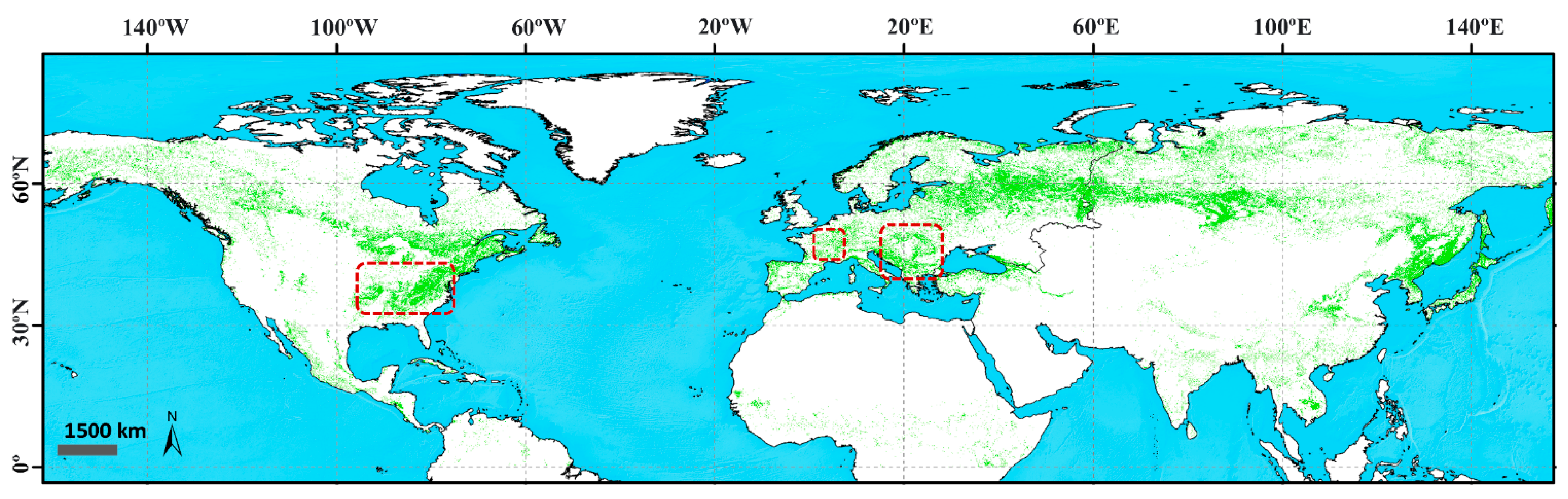
2.1.1. Study Area

Our study is focused on deciduous forests in the Northern Hemisphere (Figure 1), where the used LSP retrievals were validated [7,8]. According to the Intergovernmental Panel on Climate Change (IPCC)’s predictions [15,16], these northern regions are highly sensitive to climate change.

2.1.2. Land-Cover/vegetation Map

Because we focused on deciduous forests, we used a land-cover (LC) map that identified this type of vegetation: the Climate Change Initiative (CCI-LC) map series for 2015, at a spatial resolution of 300 m, available from the European Space Agency (ESA) [72]. CCI-LC discriminates 38 classes of land cover. We resampled the map to 0.1°, and analyzed only pixels containing deciduous forest.

2.1.3. Vegetation Phenology from SPOT VEGETATION and PROBA-V Data

The SoS and EoS during the 2000–2018 period were estimated using the time series of Copernicus Global Land Service LAI 1 km version 2, derived from SPOT VEGETATION (VGT) and PROBA-V data [73] (https://land.copernicus.eu/global/themes/vegetation (accessed on 13 June 2021)). These metrics were based on previous protocols and research [57,58,64] that used dynamic thresholds. This method is based on the percentage of the LAI amplitude in each pixel, in which the SoS is defined as the day of the year (DoY) when the LAI exceeds the 30% threshold, and the EoS is defined as the DoY when the LAI overpasses the 40% threshold after the growing season.

2.1.4. Rainfall and Temperature Datasets

The data for temperature and precipitation were collected from the ERA5 hourly gridded datasets from 2000 to 2018, with a spatial resolution of 0.25° [74]. To achieve higher resolution, we interpolated all climatological data from the spatial resolution of 0.25 to 0.1°, using a cubic convolution that calculated the value of each pixel by fitting a smooth curve based on the surrounding 16 pixels. Temperature was the air temperature at a height of 2 m, and precipitation was the accumulated amount of liquid or frozen water that fell, calculated as the sum of large-scale and convective precipitation, in millimeters.

We used the mean temperature and accumulated precipitation for the preseason, using time lags of 1, 3, and 6 months prior to the timings of the SoS and EoS.

2.1.5. SPEI

Drought indices have become useful tools for analyzing, assessing, and estimating the dry and humid periods that may have an impact on phenology [36]. Various drought indices are available, such as the Standardized Precipitation Index (SPI) or the Palmer Drought Severity Index [75] (PDSI), and several recent studies have analyzed drought conditions using the standardized precipitation evapotranspiration index (SPEI) [76,77]. The SPEI is based on precipitation and potential evapotranspiration, which includes the role of temperature in drought severity [78,79,80]. The SPEI considers drought timescales, which represent the cumulative water balance over the previous 1–48 months. It is based on the Standardized Precipitation Index (SPI) calculation method, but with improvements to include the potential evapotranspiration (PET). The SPEI uses the weekly (or monthly) difference between precipitation and PET (based on Thornthwaite’s method), and it is calculated as a standardized variable, which allows the comparison with other SPEI values and climatic variables over time and space [79]. Unlike the SPI, the SPEI includes the effects of temperature variability on drought estimation and, therefore, it takes into account the effects of warming processes on drought severity [79,80].

SPEI dataset version 2.6 was downloaded from the Global SPEI database [81] at a spatial resolution of 0.5°, and was resampled to 0.1° for the analysis. This dataset is based on the United Nations Food and Agriculture Organization (FAO)-56 Penman–Monteith estimation of potential evapotranspiration. The complete procedure for calculating the SPEI is provided by Vicente-Serrano et al. [79].

We determined drought severity for the timings of the SoS and EoS using different SPEI timescales (1, 3, 6, and 12 months), representing the cumulative water balance for the timings of preseason and presenescence. Positive SPEI values indicate that humidity is higher than the historical median, while negative values indicate a water deficit [79,80]. The SPEI data were classified into seven categories (

Table 1. Classification of drought based on SPEI data.

Range	Condition
SPEI ≤ −2	Extremely dry
−2 < SPEI ≤ −1.5	Severely dry
−1.5 < SPEI ≤ −1	Moderately dry
−1 < SPEI ≤ 1	Near normal
1 < SPEI ≤ 1.5	Moderately wet
1.5 < SPEI ≤ 2	Severely wet
SPEI ≥ 2	Extremely wet

) based on the World Atlas of Desertification [82] for analysis of conditions of wetness or dryness.

2.2. Methodology and Statistical Analysis

We first estimated the significant trends in the time series of the estimates (SoS and EoS). Secondly, we explored the impacts of anomalies in hydroclimatic variables—such as temperature, precipitation, and drought—on deciduous phenology throughout the Northern Hemisphere for 2000–2018. We applied spatiotemporal response analysis to determine the relationships between phenology and climate variables. Moreover, we investigated the spatial pattern of the sensitivity of phenology to climate, and its relationship with preseason and presenescence temperature, precipitation, and drought. We thereafter focused on some of the extreme events—including high temperatures, low temperatures, and severe drought—that have occurred in the past two decades.

We used different software to calculate and evaluate the effects of climatic variables on vegetation phenology. We first used Google Earth Engine [83] to download and process the time series of the hydroclimatic variables, and for estimating land surface phenological metrics in the Northern Hemisphere [57,58]. We then used RStudio, XLSAT, and Idrisi TerrSet for processing and statistically analyzing all data. Finally, we used ESRI ArcGIS 10.5 for generating the graphs and maps.

2.2.1. Trend Analysis

We calculated the trends in the estimated time series of the SoS and EoS before analyzing the relationships between phenology and climate. Temporal trends in the datasets were calculated by applying the Theil–Sen (TS) median slope trend analysis, which is an effective method for analyzing the rate of change in observations over a period of time (2000–2018 in our study), and is similar to linear least squares regression. TS analysis is based on nonparametric statistics (Mann–Kendall), and is independent of the assumptions of linear regression. Medians are used to calculate the trend, which is consequently less susceptible to noise and outliers [29,84,85]. The equation used to estimate the TS slope is:

$$\mathrm{TS}\mathrm{Slope}=\mathrm{Median}\left(\frac{{\mathrm{x}}_{\mathrm{j}}-{\mathrm{x}}_{\mathrm{i}}}{{\mathrm{t}}_{\mathrm{j}}-{\mathrm{t}}_{\mathrm{i}}}\right)$$

(1)

where x_j and x_i are values in years i and j, respectively. We estimated the significance of the TS slope using a nonparametric test (Mann–Kendall significance test), which provided a standardized Z and the corresponding probability (p). Positive and negative slopes indicated that the SoS and EoS had delayed and advanced trends, respectively, during the study period. The Mann–Kendall significance (Z and P) was calculated as:

$$=\{\begin{array}{c}\frac{\mathrm{S}-1}{\sqrt{\mathrm{Var}\left(\mathrm{S}\right)}} \mathrm{for} \mathrm{S}>0\\ \mathrm{j}\\ 0 \mathrm{for} \mathrm{S} =0\\ \\ \frac{\mathrm{S}+1}{\sqrt{\mathrm{Var}\left(\mathrm{S}\right)}} \mathrm{for} \mathrm{S}<0\end{array}$$

(2)

and:

$$\mathrm{P}=2\left[1-\mathsf{\varphi }\left(\left|\mathrm{z}\right|\right)\right]$$

(3)

where:

$$\mathsf{\Phi }\left(\left|\mathrm{z}\right|\right)=\frac{2}{\sqrt{\mathsf{\pi }}}\underset{0}{\overset{\left|\mathrm{z}\right|}{{\displaystyle \int }}}{\mathbf{e}}^{-{\mathrm{t}}^2}\mathrm{dt}$$

(4)

We also used the nonparametric Pettitt test method [86] to detect the possible abrupt change points in the phenological time series. This test allows us to identify shifts in the average, and their significance. The null hypothesis of the Pettitt test is the absence of a change point. The empirical significance level (p-value) was computed using XLSTAT statistical and data analysis software 2021 v.3.1, at a significance level of 5%. The nonparametric Pettitt statistical test is defined as:

$${\mathrm{K}}_{\mathsf{\tau }}=\max \left|{\mathrm{U}}_{\mathrm{t},\mathrm{T}}\right|,$$

(5)

where:

$${\mathrm{U}}_{\mathrm{t},\mathrm{T}}={\displaystyle \sum }_{\mathrm{i}=1}^{\mathrm{t}}{\displaystyle \sum }_{\mathrm{j}=\mathrm{i}+1}^{\mathrm{n}}\mathrm{sgn}\left(\mathrm{xj}-{\mathrm{x}}_{\mathrm{j}}\right)$$

(6)

where t is the period length and n is the number of data in the statistical series. The p-value and an interval around the p-value were evaluated using a Monte Carlo method.

2.2.2. Standardized Anomalies

We calculated standardized anomalies in the interannual time series (2000–2018) of phenology, temperature, and precipitation. Standardized anomalies were calculated by dividing anomalies by the standard deviation. The equation is [87]:

$$\mathrm{Z}=\frac{\mathrm{X}-\mathsf{\mu }}{\mathsf{\sigma }}$$

(7)

where Z is a standardized anomaly, X is the annual value, and µ and σ are the interannual mean and standard deviation, respectively, for each variable analyzed (i.e., the timings of the SoS and EoS, the mean preseason or presenescence temperature, or the accumulated preseason or presenescence precipitation).

Note that we estimated the anomalies in the time series of temperature and precipitation using the mean temperature and the accumulated precipitation for different timescales (1, 3, and 6 months) before estimating the timings of the SoS and EoS (see Section 2.1.3).

2.2.3. Correlation and Partial Correlation Analyses

We calculated the coefficients for the correlations between the estimated time series of phenology (SoS and EoS), temperature, precipitation, and SPEI for different preseason lengths. We used two types of correlation analysis to quantify the response of vegetation to climatic drivers. We first calculated the linear correlation (Pearson’s correlation) between the interannual anomalies of phenology (y) and hydroclimatic variables (x) at a significance level of 95%:

$${\mathrm{r}}_{\mathrm{xy}}=\frac{{\mathrm{n}\mathsf{\Sigma }\mathrm{x}}_{\mathrm{i}}{\mathrm{y}}_{\mathrm{i}}-{\mathsf{\Sigma }\mathrm{x}}_{\mathrm{i}}{\mathsf{\Sigma }\mathrm{y}}_{\mathrm{i}}}{\sqrt{\mathrm{n}{\displaystyle \sum }{\mathrm{x}}_{\mathrm{i}}^2-{\left({\mathsf{\Sigma }\mathrm{x}}_{\mathrm{i}}\right)}^2}\sqrt{\mathrm{n}{\displaystyle \sum }{\mathrm{y}}_{\mathrm{i}}^2-{\left({\mathsf{\Sigma }\mathrm{y}}_{\mathrm{i}}\right)}^2}}$$

(8)

where r_xy is the Pearson’s correlation coefficient between x and y, n is the number of observations, xi is the value of x for observation i, and yi is the value of y for observation i. A multivariate linear regression model was used for multivariate cases.

We correlated SoS and EoS anomalies with the climatic variables (temperature and precipitation) for timescales of 1, 3, and 6 months prior to the dates of the SoS and EoS, and summarized the climatic variables for the preseason periods in which the correlation was highest. For the SPEI, we used timescales from 1 to 12 months [80].

We then applied a partial correlation analysis of the SoS and EoS using the preseason and presenescence climatic variables for the three timescales (1, 3, and 6 months). The precipitation data for the same timescale were used as a constant factor for calculating the partial correlation between phenology and temperature. Similarly, the influence of temperature was considered to be a constant for calculating the correlation with accumulated precipitation. The partial correlation coefficient between vegetation and mean temperature, and its significance, were tested as:

$${\mathrm{r}}_{\mathrm{vt}.\mathrm{p}}=\frac{{\mathrm{r}}_{\mathrm{vt}}-{\mathrm{r}}_{\mathrm{vp}}{\mathrm{r}}_{\mathrm{tp}}}{\sqrt{\left(1-{\mathrm{r}}_{\mathrm{vp}}^2\right)\left(1-{\mathrm{r}}_{\mathrm{tp}}^2\right)}}$$

(9)

where v is the vegetation phenology, t is temperature, p is precipitation, and r_vt and r_vp are the simple correlation coefficients of the phenology (SoS or EoS) with the mean preseason or presenescence temperature and accumulated precipitation, respectively. Equation (8) is also valid for calculating the partial correlation between phenology and precipitation by changing the order in which the data are entered. The significance of the partial correlation coefficients at the 95% level was evaluated using Student’s t-test.

The Pearson’s correlation and partial correlation analysis produced similar maps, so the results obtained via partial correlation will be taken into account in subsequent sections for analyzing the correlations between phenology, temperature, and precipitation.

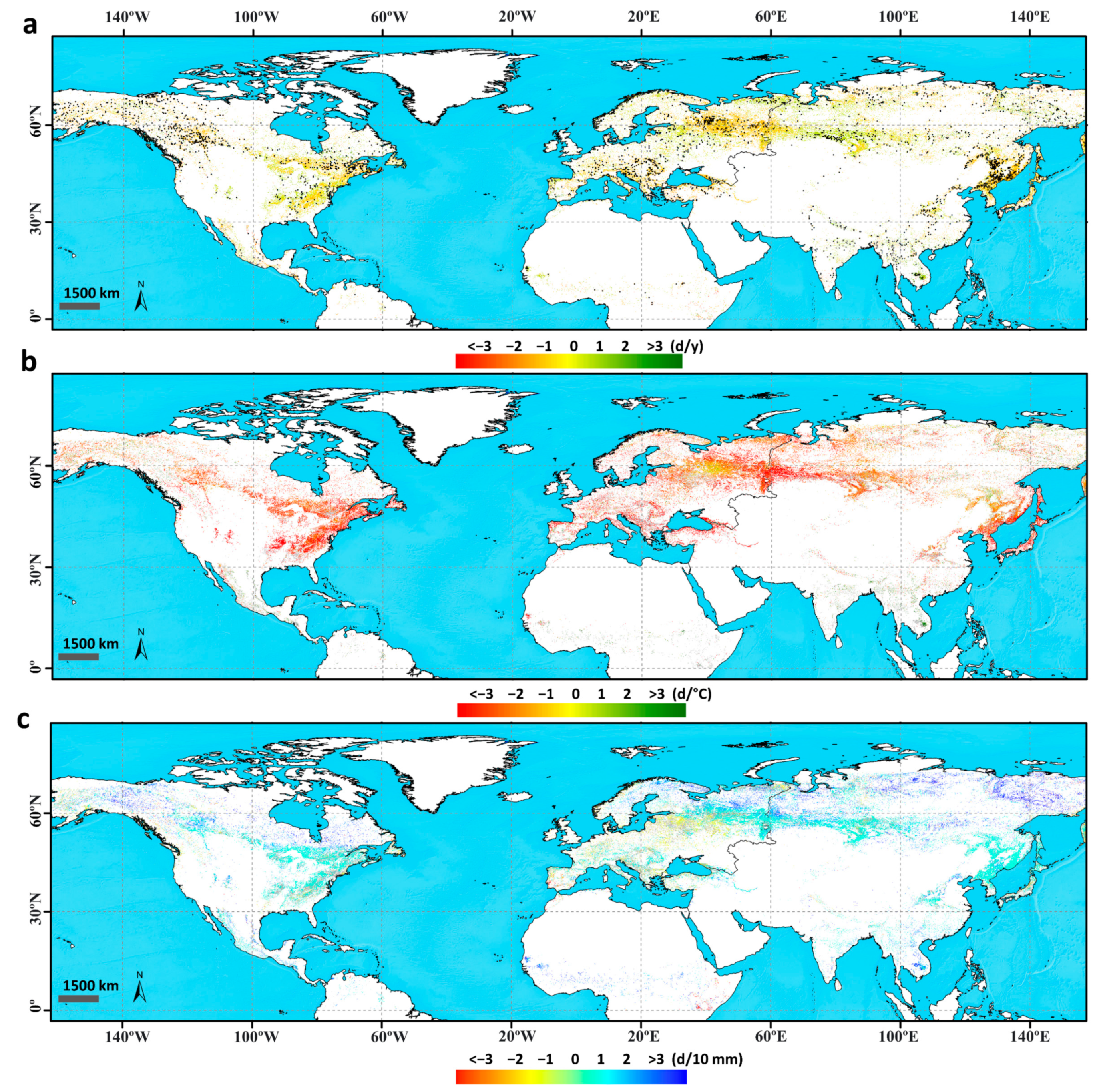
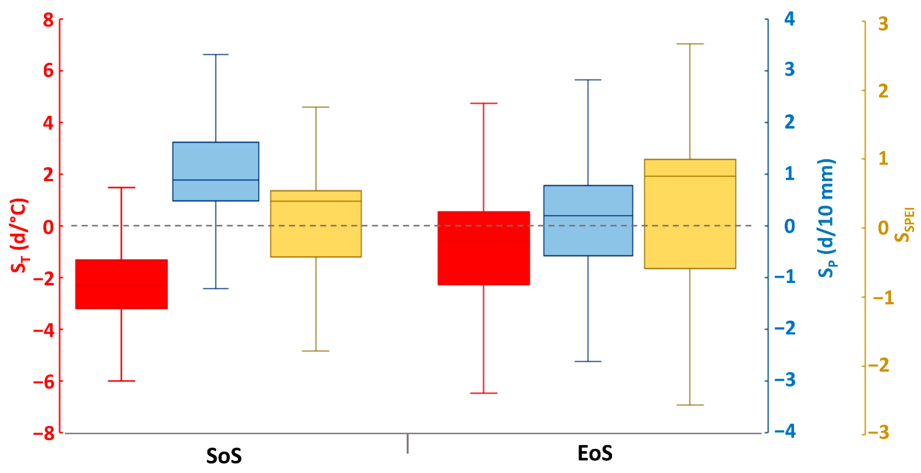
2.2.4. Sensitivity Analysis

We used multiple linear regression and sensitivity analysis to further investigate the interactions of phenology with temperature, precipitation, and SPEI. The responses of the sensitivity of vegetation phenology to the climatic variables corresponded to the slopes of the linear regressions between the phenological metrics and the climatic variables, representing the unit change in phenological date divided by the unit change in temperature, precipitation, or SPEI.

3. Results

3.1. Analysis of Trends and Correlations in the 2000–2018 Time Series

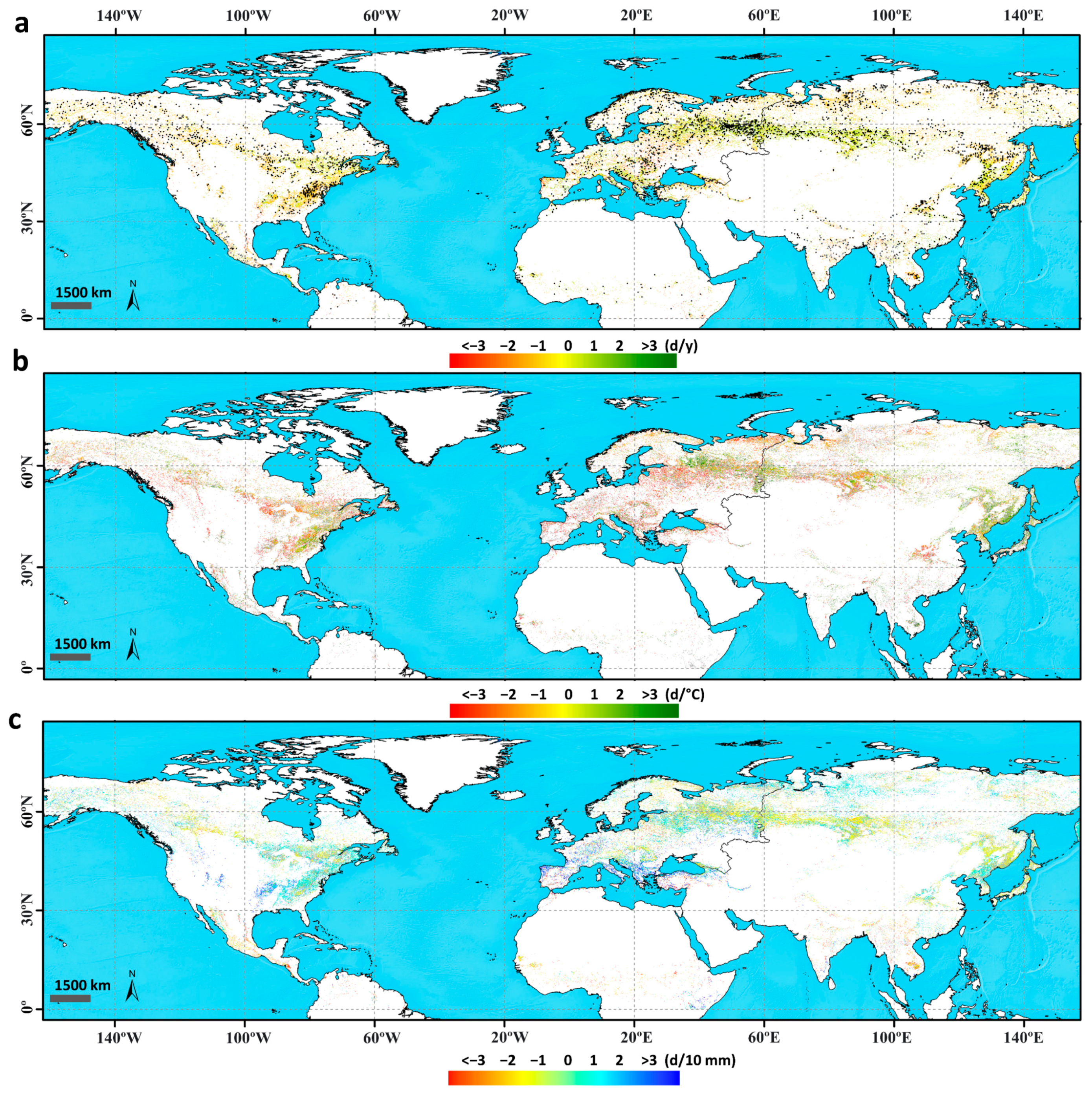
3.1.1. Trends in the Time Series of Estimated Phenology

The Pettitt test confirmed that phenological time series were monotonic, and any statistically significant change points were detected (p-values of 0.74 and 0.86 for SoS and EoS, respectively). The temporal trends in SoS for 2000–2018 (Figure 2a) were significant (p < 0.05) for 20.5% of the deciduous forests in the Northern Hemisphere. Negative trends, representing an advance in the timing of the SoS, and positive trends, representing a delay in the timing of SoS, accounted for 61.5 and 38.54% of these pixels, respectively (Table S1). Northeastern Europe mainly had negative SoS trends, while Russia and North America mainly had positive trends (Figure 1a). The EoS changed significantly in 23.8% of the deciduous forests, with 40.5 and 59.49% of these forests having a delayed and advanced EoS, respectively (Table S1). Our results indicated that the SoS and EoS advanced by 0.08 and 0.1 d/y, respectively. Positive significant trends were mainly in northeastern Europe, and negative trends were mainly in eastern North America (Figure 5a).

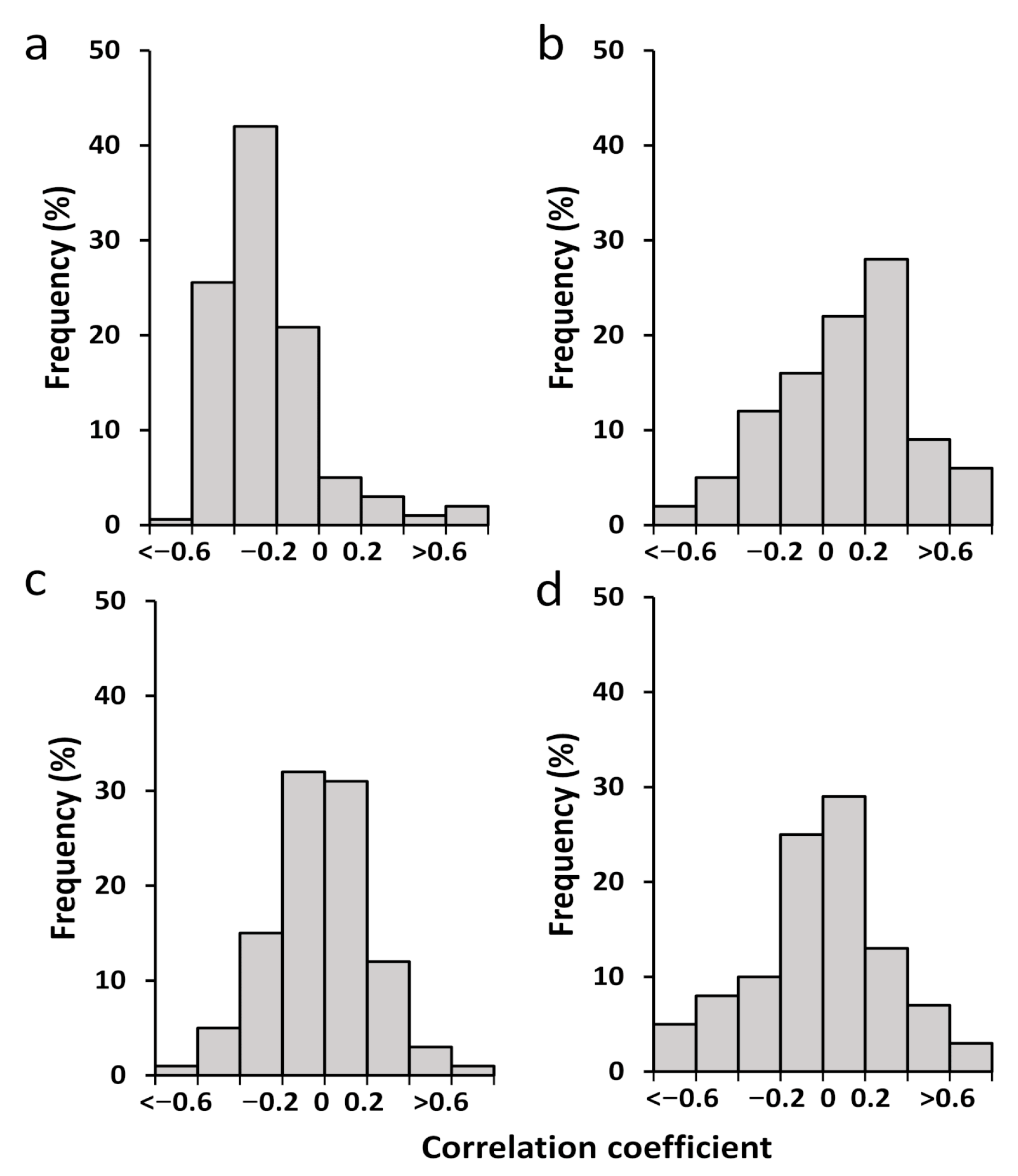
3.1.2. Correlation and Sensitivity of Phenology with Climatic Variables

The correlation between SoS anomalies and preseason temperature (Figure S1a and Figure 3) indicated that 72.13% of all pixels had significant correlations at p < 0.05, with negative correlations accounting for 57% of all pixels (

Table 2. Percentage of pixels with significant correlations (p < 0.05) between the anomalies of phenological events (SoS and EoS) and climatic variables (temperature, precipitation, and SPEI) in the Northern Hemisphere for 2000–2018.

Phenological Event	Climatic Variable	Positive (%)	Negative (%)
SoS	Temperature	14.94	57.19
	Precipitation	42.30	20.07
	SPEI	17.57	9.87
EoS	Temperature	23.57	20.75
	Precipitation	34.44	28.42
	SPEI	28.78	9.04

). An earlier SoS tended to be associated with higher temperatures in 35% of the pixels, and a later SoS was associated with lower temperatures in 21% of the pixels (Table S2). Temperature and SoS were negatively correlated in Eurasia and eastern North America, with correlation coefficients (r) of ~−0.7 and −0.6, respectively (Figure S1).

The spatial pattern of the distribution of the partial correlations between SoS and precipitation was more heterogeneous than the correlation between SoS and temperature. The correlation between SoS and precipitation was positive in most pixels, accounting for 42% of them (Table 2; Figure 3b and Figure S1b), which led to significant positive correlation advance or delay (20.9% and 21.4%) in the SoS with precipitation decrease or increase, respectively (Table S2).

The mean sensitivity of the SoS to temperature and precipitation was −2.45 d/°C and 0.8 d/10 mm, respectively (Figure 4). The sensitivity to temperature was highest (~−5 d/°C) in Eurasia and southeastern North America (Figure 2b), while the sensitivity to precipitation was highest (3 d/10 mm) at latitudes > 60° N (Figure 2c).

The sensitivity analysis (Figure 4 and Figure 5) indicated that the response of phenology to climatic anomalies was lower for the timing of the EoS than for the timing of the SoS. The pattern of temperature sensitivity was very heterogeneous, with symmetric distributions of positive and negative correlations between temperature and EoS in 23.57 and 20.75% of the pixels, respectively (Table 2, Figure 3c). EoS advanced with temperature by an average of ~0.5 d/°C (Figure 5b). The sensitivity of EoS to precipitation had the opposite pattern: the timing of EoS was delayed by an average of ~0.5 d/10 mm. Correlations were significantly positive (i.e. a delay in the timing of EoS with an increase in precipitation) in 34.44% of the study area (Figure S2), with sensitivities highest in southern and southwestern Europe (~3 d/10 mm). In contrast, 28.42% of the pixels had negative correlations (i.e., an advance in the timing of the EoS with an increase in precipitation)—mainly in northeastern Europe and areas of Russia (Figure 5c).

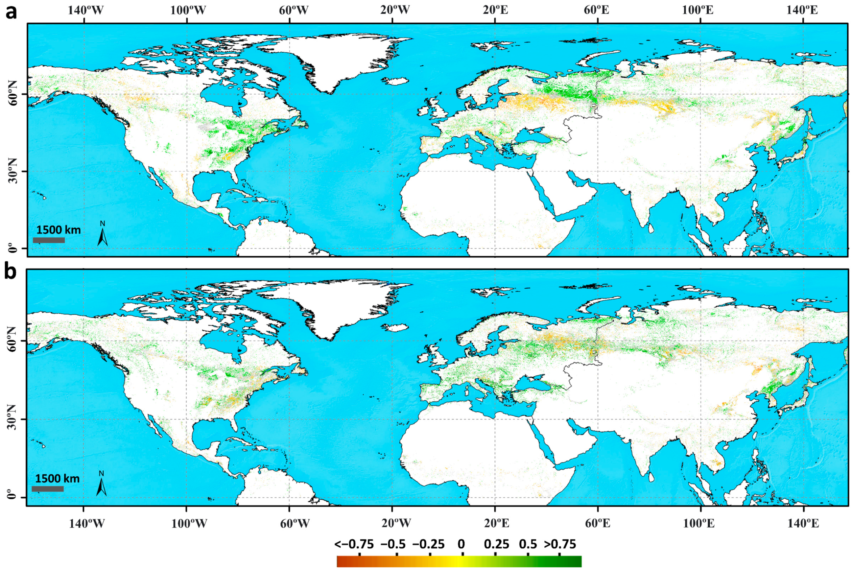
3.1.3. Response of Vegetation Phenology to Drought Using the SPEI

When analyzing the influence of drought on vegetation, we found that SPEI calculated using timescales between 1 and 3 months was the best correlated with the timings of the SoS and EoS in >50% of the pixels (Table S3).

The Spearman correlations between the SoS and the SPEI were positive in 52.3% of the Northern Hemisphere, and were significant (p < 0.05) in 17.5% of the pixels (Table 2)—mostly >60° N in northeastern Europe and North America (Figure 6a). The correlations were negative (47.6% of the pixels, significant in 9.8%) in northeastern Europe (between 50° and 60°) in areas where the sensitivity of the SoS to the SPEI was highest (Figure S3a).

Correlations between the timings of the EoS and the SPEI were positive in 58.8% of the study area (Table 2), with significant correlations for 28.8% of the pixels (p < 0.05). The correlations were particularly strong in southwestern Europe and northeastern North America (Figure 6b), in areas where the sensitivity of the EoS to the SPEI was highest (Figure S3b). Drought weakly affected phenology at high northern latitudes (>60° N), where temperature (Figure 5b), not precipitation (Figure 5c), was the main variable limiting phenology. The correlations between the EoS and the SPEI were thus weak.

3.2. Phenological Responses to Recent Climatic Extremes

We analyzed the effects of three heat- and cold waves on vegetation phenology in Europe and North America.

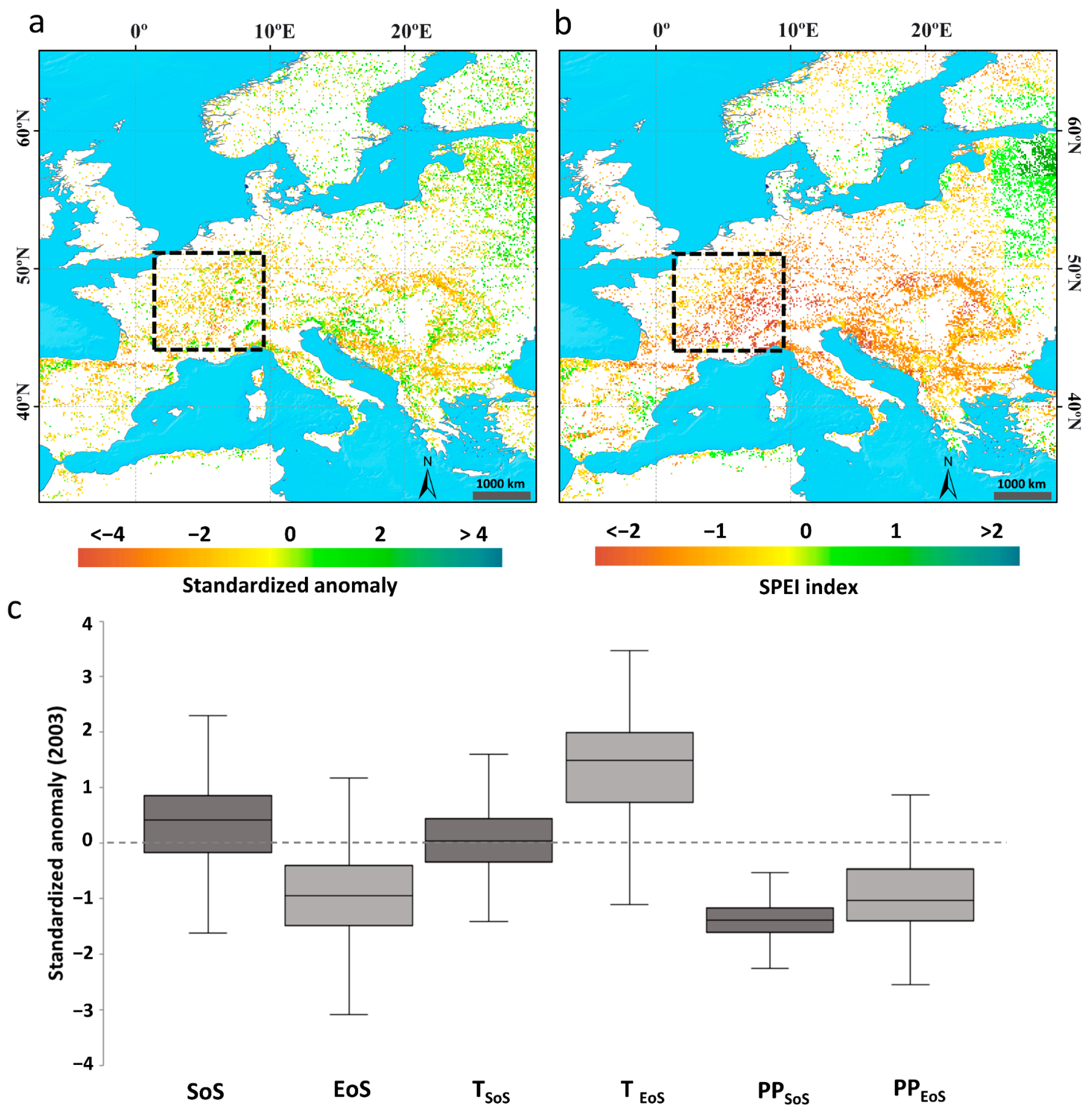
3.2.1. Effect of the 2003 Summer Heatwave in Western Europe

The year 2003 was one of the driest and warmest years recorded in the past 30 years in most of Central Europe [88,89]. The effects of this extreme episode were represented by negative anomalies in the timing of the EoS throughout most of Western Europe (Figure 7a). We highlight a region of southern France and southwestern Germany where an unstandardized anomaly for the timing of the EoS had a mean of −22 d.

An intense drought also occurred in 2003, which we identified using the SPEI (Figure 7b,

Table 3. Classification of SPEI data for characterizing drought in the three case studies: Europe, North America, and the Balkans, for 2003, 2012, and 2005, respectively. Two analytical periods are used: preseason (for the timing prior to the SoS) and presenescence (for the timing prior to the EoS). The SPEI timescale with the highest correlation in each pixel was considered.

		SoS (area, %)			EoS (area, %)
Range	Condition	Europe 2003	North America 2012	Balkans 2005	Europe 2003	North America 2012	Balkans 2005
SPEI ≤ −2	Extremely dry	0	0.77	0	26.30	3.96	0
−2 SPEI ≤ −1.5	Severely dry	2.88	9.60	0	29.75	5.56	0
−1.5 SPEI ≤ −1	Moderately dry	15.96	16.69	0	23.99	4.68	1.04
−1 < SPEI ≤ 1	Near normal	80.96	72.93	14.44	19.96	52.44	67.56
1 SPEI ≤ 1.5	Moderately wet	0	0	35.13	0	29.57	28.78
1.5 SPEI ≤ 2	Severely wet	0	0	35.08	0	3.81	2.40
SPEI ≥ 2	Extremely wet	0	0	15.35	0	0	0.23

). More than 80% of the pixels indicated an intense drought prior to the timing of the EoS. Fischer et al. [88] observed that an early EoS and stress from the lack of soil moisture contributed greatly to the suppression of evapotranspiration after the summer, and that this interaction may have amplified the temperature anomalies by locally increasing the flux of sensible heat. Figure 7c shows the standardized anomalies between phenology and the climatic variables, which allows for the visualization of the positive temperature anomalies for the timing of the EoS and the precipitation deficit for the timings of both the SoS and EoS.

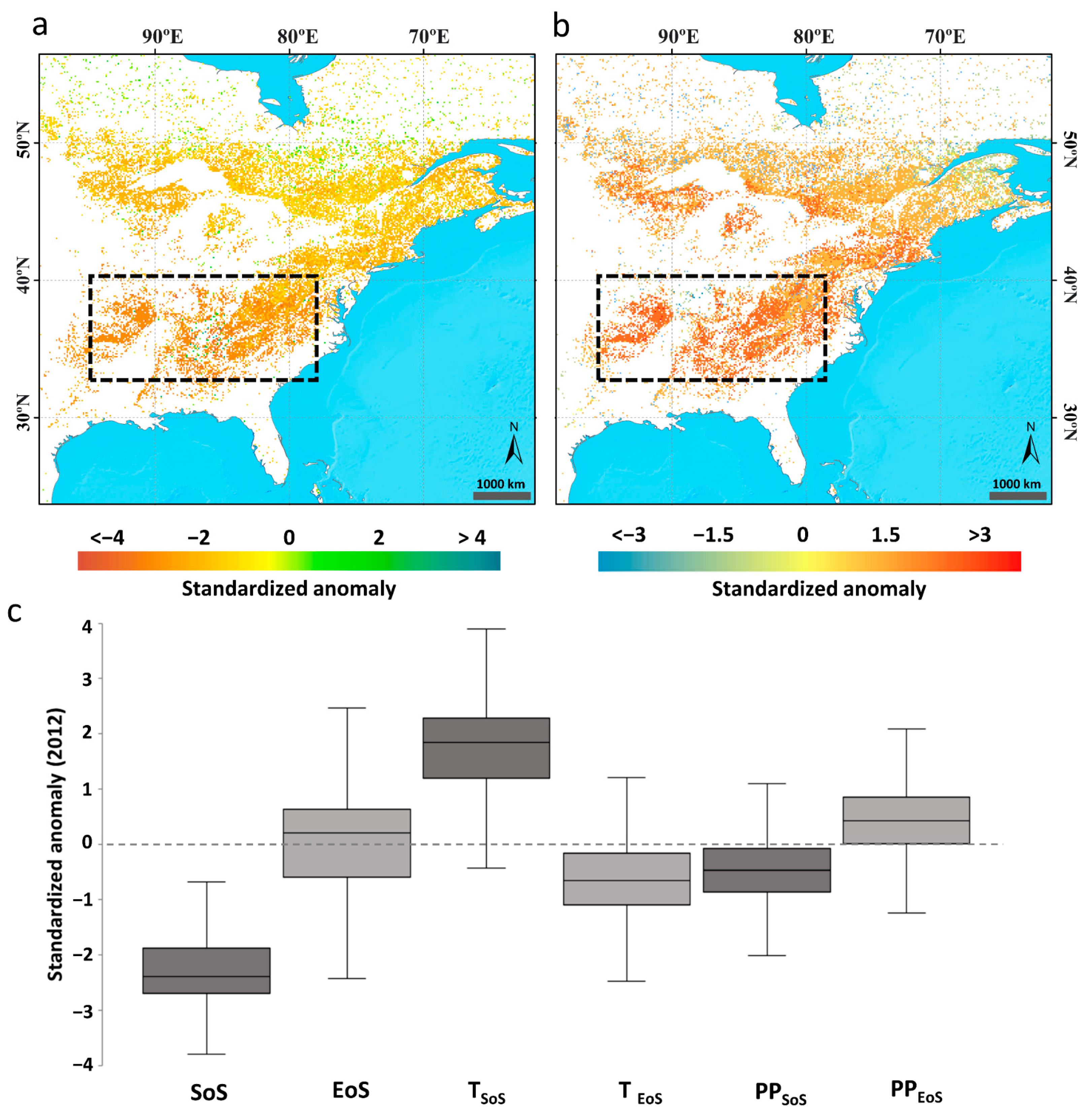
3.2.2. Effect of the 2012 Spring Heatwave in Eastern North America

We analyzed the early spring for 2012 in North America, focusing on the southeastern United States (US). We calculated the interannual anomalies for the phenological metrics and climatic variables for each pixel, in order to assess the spatial patterns of the phenological responses to the climatic extremes. Previous studies [55,56] considered the spring SoS anomaly in 2012 to be the earliest spring recorded since 1900 across North America (Figure 8a). Karl et al. [56] reported that the anomaly was driven by a strong and stable high-pressure anticyclone that remained over much of the northeast from late February to April, causing record high temperatures (Figure 8b,c) and phenological advancement.

Spring in many central and eastern areas of North America began between −15 and −30 d (unstandardized anomalies) before the mean SoS for the time series analyzed (2000–2018) (Figure 8c). The anomalies for the timing of the SoS were negative in most of the pixels (96.2%) (Figure 8a). Figure 8c shows the dominant role of temperature in the phenological advancement of the SoS in 2012, with mean standardized anomalies > 2 °C. Precipitation was slightly negatively anomalous before the timing of the SoS in 2012, but with no water stress, and the majority of the pixels (73%) indicated a normal SPEI between −1 and 1 (Table 3).

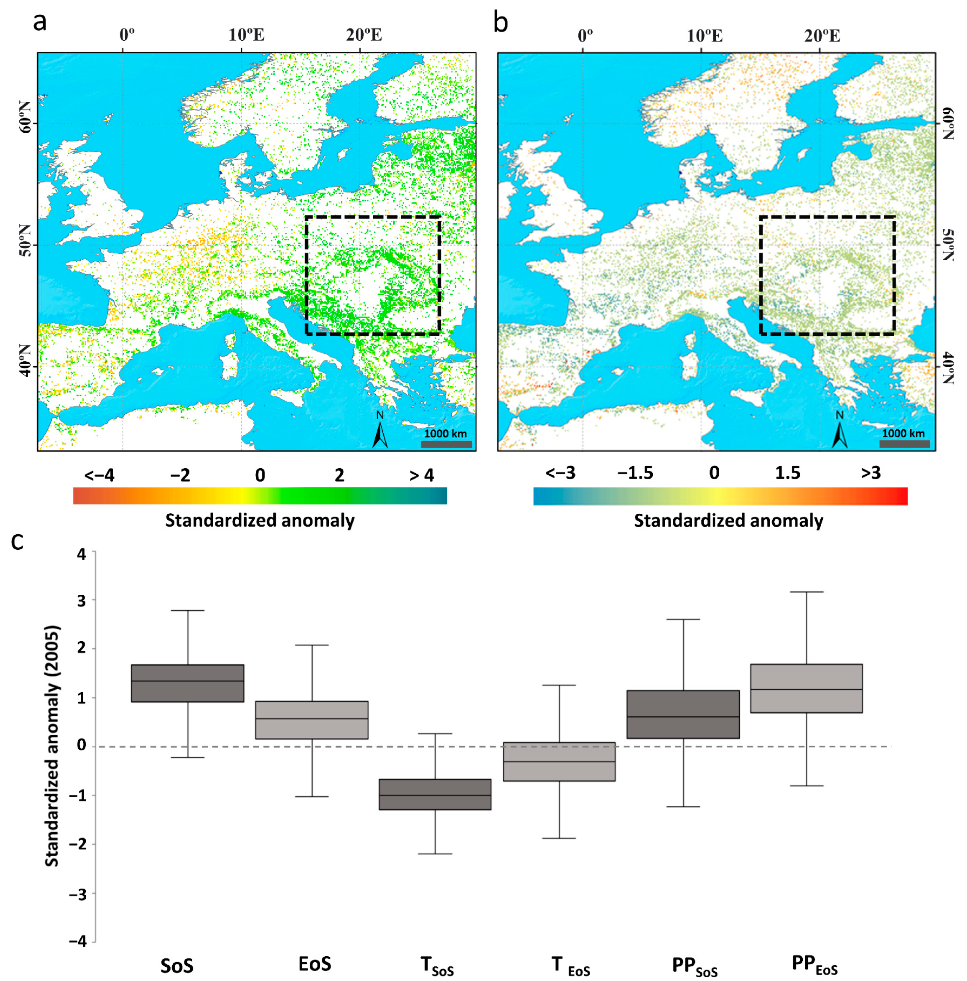
3.2.3. Effect of the Late 2005 Cold Wave in the Balkans

Unlike the two previous analyses, this third case refers to a delayed SoS due to a negative temperature anomaly for the timing of the preseason. Figure 9a,b shows the SoS anomaly and preseason mean temperature for 2005, respectively. The positive anomalies of the SoS affected much of Central and Eastern Europe—especially the northern Balkan Peninsula and the Carpathian Mountains, where positive anomalies were 10 d in most of the pixels (80.3%) (Figure 9a,c). The average standardized temperature anomaly was ~−1 °C (Figure 9b,c), which greatly delayed the timing of the SoS (~10 d). This delay also coincided with a positive SPEI. Eighty percent of the pixels represented moderate or very high humidities prior to the SoS (Table 3).

4. Discussion

Climatic projections indicate a likely increase in temperatures in much of the world, especially at the higher latitudes of the Northern Hemisphere [9,10]. Recent studies [12,90] have also found that extreme climatic events have increased in frequency, intensity, and duration—consistent with IPCC projections—which will affect many ecosystems, and especially vegetation. Climatic variability adds uncertainty in analyzing and predicting the impacts of climate change on vegetation phenology [3,38,91].

Previous studies have attributed the recent shifts in phenology to climate change, and to the effects of variations in temperature and precipitation [15,16,17,92]. Assessing the pattern of distribution, the variability of phenology, and the correlations between phenology and climatic variables is crucial for understanding the potential effects of future climate change [93]. Remotely sensed data have been widely used to assess trends in phenological time series and their responses to climatic variability. Numerous studies have reported that the phenological trends from 2000 to 2018 were lower than the rates of change from 1980 to 1999 [14,94,95,96]. De Beurs et al. [15] and Piao et al. [28] reported that the SoS advanced by 6.6 and 7.9 d/decade in North America and China, respectively, between 1982 and 1999. Jeong et al. [14] and Zeng et al. [95], however, found that phenological trends declined significantly after 2000, with an advancement of the timing of the SoS of 0.1–0.2 d/decade, respectively—consistent with our results. Some studies have even reported delays of 1 d/decade in the timing of the SoS after 2000, specifically in western North America [94,96].

In our study, we used land surface phenological metrics at the continental scale derived from LAI time series (2000–2018) of the SPOT-VGT and PROBA-V sensors [57,58]. Since the time series start in 2000, the detected trends are limited to reduced areas. For this reason, we mainly focused on analyzing the correlations between phenology and climatic variables, and analyzing the responses of phenological anomalies to recent climatic events.

Most previous studies have only emphasized the role of preseason temperature in determining the SoS, because an increase in the advance of the SoS is a consequence of global warming [8,28,29,97,98,99]. Other studies focusing on the EoS have recorded a delay in senescence, which led to longer growing seasons in some areas of Eurasia and North America [14,100]. We focused on analyzing the responses of phenology to mean preseason and presenescence temperatures, accumulated precipitation, and drought across the deciduous forests in the Northern Hemisphere. Our results indicated that anomalies of temperature and precipitation controlled the changes in phenological metrics in the deciduous forests, consistent with previous studies [2,101]; the anomalies of SoS were particularly strongly associated with the changes in mean preseason temperature, so this climatic variable may have been the main cause of the advance or delay in the start of the growing season, affecting 72.1% of the study area (mean r of −0.31) (p < 0.05). Correlations were significantly negative in 57% of the pixels (p < 0.05), i.e., an advance or delay in the SoS due to higher or lower temperatures, respectively.

The effects of the relationships between the climatic variables and vegetation on the timing of the EoS were more complex. The timing of the end of the growing season in response to temperature was generally delayed in most pixels. Water stress associated with droughts during summer, however, advanced the EoS in some regions—such as Southern Europe (Figure S2 and Figure 6)—with negative anomalies longer than −20 d for the timing of the EoS throughout most of Europe (in 2003), consistent with other studies [102,103,104,105].

The influence of drought on the timing of the EoS was lower in humid and cold regions (such as those pixels located between 55 and 80° N) than in drier regions, such as areas with a Mediterranean climate (Figure S3). The availability of water in Mediterranean areas was the primary limiting resource for the timing of the EoS, but temperature and other variables—such as photoperiod—may play a larger role at higher latitudes.

The distribution of the regression coefficients between the anomalies in phenology and the climatic variables was highly spatially heterogeneous, due to the spatial and latitudinal heterogeneity in climate, as well as the biological characteristics of the species, which could account for the variable responsiveness to climate [25,106]. The responses of phenology to climate—especially to climatic extremes—also vary with climatic gradients, type of event, and biome, and even among individuals of the same species [38,91].

These phenological changes may affect climate change via the feedback between vegetation and climate [1,3,107,108,109]. For example, climatic anomalies or extremely high temperatures (such as during heatwaves) alter vegetation growth due to both the high temperatures and lower amounts of soil moisture [47,51,110]. Altered vegetation growth greatly affects the uptake of CO₂, depending on the availability of soil water, regional characteristics, and plant species [3]. Deficits in soil moisture lead to lower water evaporation, which lowers the release of latent heat from the land, prevents the development of clouds, and may consequently intensify droughts because precipitation is reduced [111,112,113], which could also involve teleconnections between areas [109].

5. Conclusions

This study comprehensively analyzed the response of vegetation to climatic anomalies in the Northern Hemisphere, and assessed the impact of extreme climatic events on deciduous phenology. Our results suggest that deciduous phenology in the Northern Hemisphere is very sensitive to shifts in temperature—especially for the timing of the SoS—but also indicate the importance of water availability to the timing of the EoS, as the increase in drought stress contributes to its advance throughout some regions (e.g., Southern Europe). Our results also revealed that extreme climate events exert severe impacts on vegetation phenology for the timing of both the SoS and EoS. These findings highlight the need to develop strategies focused on mitigating the impact of future climate changes on vegetation, and their monitoring. The interactions of temperature, precipitation, drought, and phenology with other variables—such as solar radiation, soil type, soil moisture, and the coupling between variables and feedback between vegetation and climate—warrant future research.

References

1. Ceccherini, G.; Gobron, N.; Migliavacca, M. On the Response of European Vegetation Phenology to Hydroclimatic Anomalies. Remote Sens. 2014, 6, 3143–3169. [Google Scholar] [CrossRef] [Green Version]
2. He, Z.; Du, J.; Chen, L.; Zhu, X.; Lin, P.; Zhao, M.; Fang, S. Impacts of recent climate extremes on spring phenology in arid-mountain ecosystems in China. Agric. For. Meteorol. 2018, 260, 31–40. [Google Scholar] [CrossRef]
3. Peñuelas, J.; Filella, I. Phenology feedbacks on climate change. Science 2009, 324, 887–888. [Google Scholar] [CrossRef] [Green Version]
4. Richardson, A.D.; Keenan, T.F.; Migliavacca, M.; Ryu, Y.; Sonnentag, O.; Toomey, M. Climate change, phenology, and phenological control of vegetation feedbacks to the climate system. Agric. For. Meteorol. 2013, 169, 156–173. [Google Scholar] [CrossRef]
5. White, M.A.; Hoffman, F.; Hargrove, W.W. A global framework for monitoring phenological responses to climate change. Geophys. Res. Lett. 2005, 32. [Google Scholar] [CrossRef] [Green Version]
6. Walther, G.R.; Post, E.; Convey, P.; Menzel, A.; Parmesan, C.; Beebee, T.J.; Fromentin, J.M.; Hoegh-Guldberg, O.; Bairlein, F. Ecological responses to recent climate change. Nature 2002, 416, 389–395. [Google Scholar] [CrossRef]
7. Bradley, A.V.; Gerard, F.F.; Barbier, N.; Weedon, G.P.; Anderson, L.O.; Huntingford, C.; Aragao, L.E.; Zelazowski, P.; Arai, E. Relationships between phenology, radiation and precipitation in the Amazon region. Glob. Chang. Biol. 2011, 17, 2245–2260. [Google Scholar] [CrossRef]
8. Cleland, E.; Chuine, I.; Menzel, A.; Mooney, H.A.; Schwartz, M.D. Shifting plant phenology in response to global change. Trends Ecol. Evol. 2017, 22, 357–365. [Google Scholar] [CrossRef] [PubMed]
9. IPCC. Climate Change 2012. Managing the Risks of Extreme Events and Disasters to Advance Climate Change Adaptation. A Special Report of Working Groups I and II of the Intergovernmental Panel on Climate Change; Field, C.B., Barros, V., Stocker, T.F., Qin, D., Dokken, D.J., Eds.; Cambridge University Press: Cambridge, UK; New York, NY, USA, 2012; p. 582. [Google Scholar]
10. IPCC. Climate Change 2007. Contribution of Working Group 1 to the Fourth Assessment Report of the Intergovernmental Panel on Climate Change; Solomon, S., Qin, M., Manning, Z., Chen, M., Marquis, K.B., Eds.; Cambridge University Press: Cambridge, UK; New York, NY, USA, 2007. [Google Scholar]
11. IPCC. Climate Change 2013: The Physical Science Basis. Contribution of Working Group I to the Fifth Assessment Report of the Intergovernmental Panel on Climate Change; Stocker, T.F., Qin, D., Plattner, G.-K., Tignor, M., Allen, S.K., et al., Eds.; Cambridge University Press: Cambridge, UK, 2013; p. 1535. [Google Scholar]
12. Du, J.; He, Z.; Piatek, K.; Chen, L.F.; Lin, P.; Zhu, X. Interacting effects of temperature and precipitation on climatic sensitivity of spring vegetation green-up in arid mountains of China. Agric. For. Meteorol. 2019, 269, 71–77. [Google Scholar] [CrossRef]
13. Piao, S.L.; Friedlingstein, P.; Ciais, P.; Viovy, N.; Demarty, J. Growing season extension and its effects on terrestrial carbon flux over the last two decades. Glob. Biogeochem. Cycles 2007, 21, GB3018. [Google Scholar] [CrossRef]
14. Jeong, S.J.; Ho, C.H.; Gim, H.J.; Brown, M. Phenology shifts at start vs end of growing season in temperate vegetation over the Northern Hemisphere for the period 1982–2008. Glob. Chang. Biol. 2011, 17, 2385–2399. [Google Scholar] [CrossRef]
15. De Beurs, K.; Henebry, G. Land surface phenology and temperature variation in the International Geosphere–Biosphere Program high-latitude transects. Glob. Chang. Biol. 2005, 11, 779–790. [Google Scholar] [CrossRef]
16. Zhou, L.; Tucker, C.J.; Kaufmann, R.K.; Slayback, D.; Shabanov, N.V.; Myneni, R.B. Variations in northern vegetation activity inferred from satellite data of vegetation index during 1981–1999. J Geophys. Res. 2001, 106, 20069–20083. [Google Scholar] [CrossRef]
17. Shen, M.G.; Piao, S.L.; Cong, N.; Zhang, G.X.; Jassens, I.A. Precipitation impacts on vegetation spring phenology on the Tibetan Plateau. Glob. Chang. Biol. Bioenergy 2015, 21, 3647–3656. [Google Scholar] [CrossRef] [PubMed] [Green Version]
18. Forrest, J.; Miller-Rushing, A.J. Toward a synthetic understanding of the role of phenology in ecology and evolution. Philos. Trans. R. Soc. 2010, 365, 3101–3112. [Google Scholar] [CrossRef] [PubMed] [Green Version]
19. Cong, N.; Shen, M.G.; Piao, S.L. Spatial variations in responses of vegetation autumn phenology to climate change on the Tibetan Plateau. J. Plant Ecol. 2017, 10, 744–752. [Google Scholar] [CrossRef] [Green Version]
20. Thackeray, S.J.; Henrys, P.A.; Hemming, D.; Bell, J.R.; Botham, M.S.; Burthe, S.; Helaouet, P.; Johns, D.G.; Jones, I.D.; Leech, D.I.; et al. Phenological sensitivity to climate across taxa and trophic levels. Nature 2016, 535, 241–245. [Google Scholar] [CrossRef] [PubMed] [Green Version]
21. Wang, W.; Anderson, B.; Entekhabi, D.; Huang, D.; Su, Y.; Kaufmann, R.; Myneni, R. Intraseasonal interactions between temperature and vegetation over the boreal forests. Earth Interact. 2007, 11, 1–30. [Google Scholar] [CrossRef] [Green Version]
22. Forzieri, G.; Feyen, L.; Cescatti, A.; Vivoni, E.R. Spatial and temporal variations in ecosystem response to monsoon precipitation variability in southwestern North America. J. Geophys. Res. 2014, 119, 1999–2017. [Google Scholar] [CrossRef] [Green Version]
23. Estrella, N.; Menzel, A. Responses of leaf colouring in four deciduous tree species to climate and weather in Germany. Clim. Res. 2006, 32, 253–267. [Google Scholar] [CrossRef] [Green Version]
24. Lu, P.L.; Yu, Q.; Liu, J.D.; He, Q.T. Effects of changes in spring temperature on flowering dates of woody plants across China. Bot. Stud. 2016, 47, 153–161. [Google Scholar]
25. Peñuelas, J.; Filella, I.; Comas, P. Changed plant and animal life cycles from 1952 to 2000 in the Mediterranean region. Glob. Chang. Biol. 2002, 8, 531–544. [Google Scholar] [CrossRef] [Green Version]
26. Peñuelas, J.; Filella, I. Phenology: Responses to a warming world. Science 2001, 294, 793–795. [Google Scholar] [CrossRef] [PubMed]
27. Piao, S.; Liu, Q.; Chen, A.; Janssens, I.A.; Fu, Y.; Dai, J.; Liu, L.; Lian, X.; Shen, M.; Zhu, X. Plant phenology and global climate change: Current progresses and challenges. Glob. Chang. Biol. 2019, 25, 1922–1940. [Google Scholar] [CrossRef] [PubMed]
28. Piao, S.; Fang, J.; Zhou, L.M.; Ciais, P.; Zhu, B. Variations in satellite-derived phenology in China’s temperate vegetation. Glob. Change Biol. 2006, 12, 672–685. [Google Scholar] [CrossRef]
29. Kang, W.; Wang, T.; Liu, S. The Response of Vegetation Phenology and Productivity to Drought in Semi-Arid Regions of Northern China. Remote Sens. 2018, 10, 727. [Google Scholar] [CrossRef] [Green Version]
30. Menzel, A. Plant phenological anomalies in Germany and their relation to air temperature and NAO. Clim. Change 2003, 57, 243–263. [Google Scholar] [CrossRef]
31. Piao, S.; Wang, X.; Ciais, P.; Zhu, B.; Wang, T.; Liu, J. Changes in satellite-derived vegetation growth trend in temperate and Boreal Eurasia from 1982 to 2006. Glob. Chang. Biol. 2011, 17, 3228–3239. [Google Scholar] [CrossRef]
32. Piao, S.; Tan, J.; Chen, A.; Fu, Y.H.; Ciais, P.; Liu, Q.; Janssens, I.A.; Vicca, S.; Zeng, Z.; Jeong, S.J.; et al. Leaf onset in the northern hemisphere triggered by daytime temperature. Nat. Commun. 2015, 6, 6911. [Google Scholar] [CrossRef] [Green Version]
33. Ramos, A.; Pereira, M.J.; Soares, A.; Rosário, L.d.; Matos, P.; Nunes, A.; Branquinho, C.; Pinho, P. Seasonal patterns of Mediterranean evergreen woodlands (Montado) are explained by long term precipitation. Agric. For. Meteorol. 2015, 202, 44–50. [Google Scholar] [CrossRef]
34. Chen, H.; Sun, J. Changes in drought characteristics over China using the standardized precipitation evapotranspiration index. J. Clim. 2015, 28, 5430–5447. [Google Scholar] [CrossRef]
35. Held, I.M.; Soden, B. Robust responses of the hydrological cycle to global warming. J. Clim. 2006, 19, 5686–5699. [Google Scholar] [CrossRef]
36. Javed, T.; Li, Y.; Feng, K.; Ayantobo, O.O.; Ahmad, S.; Chen, X.; Rashid, S.; Suon, S. Monitoring responses of vegetation phenology and productivity to extreme climatic conditions using remote sensing across different sub-regions of China. Environ. Sci. Pollut. Res. 2021, 28, 3644–3659. [Google Scholar] [CrossRef] [PubMed]
37. Sheffield, J.; Wood, E. Projected changes in drought occurrence under future global warming from multi-model, multi-scenario, IPCC AR4 simulations. Clim. Dyn. 2008, 31, 79–105. [Google Scholar] [CrossRef]
38. Ma, X.; Huete, A.; Moran, S.; Ponce-Campos, G.; Eamus, D. Abrupt shifts in phenology and vegetation productivity under climate extremes. J. Geophys. Res. Biogeosci. 2015, 120, 2036–2052. [Google Scholar] [CrossRef]
39. Butt, N.; Seabrook, L.; Maron, M.; Law, B.S.; Dawson, T.P.; Syktus, J.; McAlpine, C.A. Cascading effects of climate extremes on vertebrate fauna through changes to low-latitude tree flowering and fruiting phenology. Glob. Chang. Biol. 2015, 21, 3267–3277. [Google Scholar] [CrossRef] [Green Version]
40. Menzel, A.; Seifert, H.; Estrella, N. Effects of recent warm and cold spells on European plant phenology. Int. J. Biometeorol. 2011, 55, 921–932. [Google Scholar] [CrossRef]
41. Jentsch, A.; Kreyling, J.; Boettcher, J.; Beierkuhnlein, C. Beyond gradual warming: Extreme weather events alter flower phenology of European grassland and heath species. Glob. Chang. Biol. 2009, 15, 837–849. [Google Scholar] [CrossRef]
42. Reichstein, M.; Bahn, M.; Ciais, P.; Frank, D.; Mahecha, M.D.; Seneviratne, S.I.; Zscheischler, J.; Beer, C.; Buchmann, N.; Frank, D.C.; et al. Climate extremes and the carbon cycle. Nature 2013, 500, 287–295. [Google Scholar] [CrossRef] [PubMed]
43. Tang, X.G.; Li, H.P.; Ma, M.G.; Yao, L.; Peichl, M.; Arain, A.; Xu, X.B.; Goulden, M. How do disturbances and climate effects on carbon and water fluxes differ between multi-aged and even-aged coniferous forests? Sci. Total Environ. 2017, 599, 1583–1597. [Google Scholar] [CrossRef]
44. Zheng, C.; Tang, X.; Gu, Q.; Wang, T.; Wei, J.; Song, L.; Ma, M. Climatic anomaly and its impact on vegetation phenology, carbon sequestration and water-use efficiency at a humid temperate forest. J. Hydrol. 2018, 565. [Google Scholar] [CrossRef]
45. Zhao, A.; Zhang, A.; Cao, S.; Liu, X.F.; Liu, J.H.; Cheng, D. Responses of vegetation productivity to multi-scale drought in Loess Plateau, China. Catena 2018, 163, 165–171. [Google Scholar] [CrossRef]
46. Ivits, E.; Horion, S.; Fensholt, R.; Cherlet, M. Drought footprint on European ecosystems between 1999 and 2010 assessed by remotely sensed vegetation phenology and productivity. Glob. Chang. Biol. 2014, 20, 581–593. [Google Scholar] [CrossRef] [PubMed]
47. Reichstein, M.; Ciais, P.; Papale, D.; Valentini, R.; Running, S.; Viovy, N.; Cramer, W.; Granier, A.; Ogée, J.; Allard, V.; et al. Reduction of ecosystem productivity and respiration during the European summer 2003 climate anomaly: A joint flux tower, remote sensing and modelling analysis. Glob. Chang. Biol. 2007, 13, 634–651. [Google Scholar] [CrossRef]
48. Ponce-Campos, G.; Moran, M.; Huete, A.; Zhang, Y.; Bresloff, C.; Huxman, T.; Starks, P. Ecosystem resilience despite large-scale altered hydroclimatic conditions. Nature 2013, 494, 349–352. [Google Scholar] [CrossRef] [PubMed]
49. Fischer, E.M.; Schär, C. Consistent geographical patterns of changes in high-impact European heatwaves. Nat. Geosci. 2010, 3, 398–403. [Google Scholar] [CrossRef]
50. Trumbore, S.; Brando, P.; Hartmann, H. Forest health and global change. Science 2015, 349, 814–818. [Google Scholar] [CrossRef] [Green Version]
51. Ciais, P.; Reichstein, M.; Viovy, N.; Granier, A.; Ogée, J.; Allard, V.; Aubinet, M.; Buchmann, N.; Bernhofer, C.; Carrara, A.; et al. Europe-wide reduction in primary productivity caused by the heat and drought in 2003. Nature 2005, 437, 529–533. [Google Scholar] [CrossRef]
52. Gobron, N.; Pinty, B.; Mélin, F.; Taberner, M.; Verstraete, M.; Belward, A.; Lavergne, T.; Widlowski, J.L. The state of vegetation in Europe following the 2003 drought. Int. J. Remote Sens. 2005, 26, 2013–2020. [Google Scholar] [CrossRef]
53. Lorenz, R.; Davin, E.; Lawrence, D.; Stöckli, R.; Seneviratne, S. How important is vegetation phenology for European climate and heatwaves? J. Clim. 2013, 26, 10077–10100. [Google Scholar] [CrossRef] [Green Version]
54. Diffenbaugh, N. Sensitivity of extreme climate events to CO2 induced biophysical atmosphere-vegetation feedbacks in the western United States. Geophys. Res. Lett. 2005, 32, 1–4. [Google Scholar] [CrossRef]
55. Ellwood, E.; Temple, S.; Primack, R.; Bradley, N.; Davis, C. Record-Breaking Early Flowering in the Eastern United States. PLoS ONE 2013, 8, e53788. [Google Scholar] [CrossRef] [PubMed]
56. Karl, T.R.; Gleason, B.; Menne, M.; Mcmahon, J.; Heim, J.; Brewer, M.; Kunkel, K.; Arndt, D.; Privette, J.; Bates, J.; et al. temperature and drought: Recent anomalies and trends. EoS Trans. 2012, 93, 473–474. [Google Scholar] [CrossRef]
57. Bórnez, K.; Descals, A.; Verger, A.; Peñuelas, J. Land surface phenology from VEGETATION and PROBA-V data. Assessment over deciduous forests. Int. J. Appl. Earth Obs. Geoinf. 2020, 84, 101974. [Google Scholar] [CrossRef]
58. Bórnez, K.; Richardson, A.D.; Verger, A.; Descals, A.; Peñuelas, J. Evaluation of VEGETATION and PROBA-V Phenology Using PhenoCam and Eddy Covariance Data. Remote Sens. 2020, 12, 3077. [Google Scholar] [CrossRef]
59. Richardson, A.D.; Braswell, B.; Hollinger, D.Y.; Jenkins, J.P.; Ollinger, S.V. Near-surface remote sensing of spatial and temporal variation in canopy phenology. Ecol. Appl. 2009, 19, 1417–1428. [Google Scholar] [CrossRef]
60. Wang, S.; Yang, B.; Yang, Q.; Lu, L.; Wang, X.; Peng, Y. Temporal Trends and Spatial Variability of Vegetation Phenology over the Northern Hemisphere during 1982–2012. PLoS ONE. 2016, 11, e0157134. [Google Scholar] [CrossRef] [PubMed]
61. Verger, A.; Baret, F.; Weiss, M. Algorithm Theoretical Basis Document: LAI, FAPAR, FCOVER Collection 1km, Version 2, Issue I1.41. 2019. Available online: https://land.copernicus.eu/global/sites/cgls.vito.be/files/products/CGLOPS1_ATBD_LAI1km-V2_I1.41.pdf (accessed on 10 July 2020).
62. Atkinson, P.M.; Jeganathan, C.; Dash, J.; Atzberger, C. Inter-comparison of four models for smoothing satellite sensor time-series data to estimate vegetation phenology. Remote Sens. Environ. 2012, 123, 400–417. [Google Scholar] [CrossRef]
63. Delbart, N.; Kergoat, L.; Le Toan, T.; Lhermitte, J.; Picard, G. Determination of phenological dates in boreal regions using Normalized Difference Water Index. Remote Sens. Environ. 2005, 97, 26–38. [Google Scholar] [CrossRef] [Green Version]
64. Verger, A.; Filella, I.; Baret, F.; Penuelas, J. Vegetation baseline phenology from kilometric global LAI satellite products. Remote Sens. Environ. 2016, 178, 1–14. [Google Scholar] [CrossRef] [Green Version]
65. Zhang, X.; Friedl, M.A.; Schaaf, C.B. Climate controls on vegetation phenological patterns in northern mid- and high latitudes inferred from MODIS data. Glob. Change Biol. 2004, 10, 1133–1145. [Google Scholar] [CrossRef]
66. Menzel, A.; Fabian, P. Growing season extended in Europe. Nature 1999, 397, 659. [Google Scholar] [CrossRef]
67. Beaubien, E.G.; Freeland, H.J. Spring phenology trends in Alberta, Canada: Links to ocean temperature. Int. J. Biom. 2000, 44, 53–59. [Google Scholar] [CrossRef]
68. Chmielewski, F.M.; Rotzer, T. Annual and spatial variability of the beginning of growing season in Europe in relation to air temperature changes. Clim. Res. 2002, 19, 257–264. [Google Scholar] [CrossRef] [Green Version]
69. Schwartz, M.D.; Ahas, R.; Aasa, A. Onset of spring starting earlier across the Northern Hemisphere. Glob. Chang. Biol. 2006, 12, 343–351. [Google Scholar] [CrossRef]
70. Julien, Y.; Sobrino, J. Global land surface phenology trends from GIMMS database. Int. J. Remote Sens. 2009, 30, 3495–3513. [Google Scholar] [CrossRef] [Green Version]
71. White, M.A.; de Beurs, K.; Didan, K.; Inouye, D.; Richardson, A.; Jensen, O.; Lauenroth, W. Intercomparison, interpretation, and assessment of spring phenology in North America estimated from remote sensing for 1982–2006. Glob. Chang. Biol. 2009, 15, 2335–2359. [Google Scholar] [CrossRef]
72. ESA. Land Cover CCI Product C3S. Available online: http://maps.elie.ucl.ac.be/CCI/viewer/download.php (accessed on 2 May 2021).
73. Verger, A.; Baret, F.; Weiss, M. Near real time vegetation monitoring at global scale. IEEE J. Sel. Top. Appl. Earth Obs. Remote Sens. 2014, 7, 3473–3481. [Google Scholar] [CrossRef]
74. ERA5 Climate Dataset. Available online: https://cds.climate.copernicus.eu/ (accessed on 2 May 2021).
75. Palmer, W.C. Meteorological drought. U.S. Research Paper No. 45; US Weather Bureau: Washington, DC, USA, 1965; p. 58.
76. Chen, S.; Zhang, L.G.; Tang, R.; Yang, K.; Huang, Y. Analysis on temporal and spatial variation of drought in Henan Province based on SPEI and TVDI. Trans. Chin. Soc. Agric. Eng. 2017, 33, 126–132. [Google Scholar]
77. Wang, Z.; Li, J.; Lai, C.; Huang, Z.; Zhong, R.; Zeng, Z.; Chen, X. Increasing drought has been observed by SPEI_pm in Southwest China during 1962–2012. Theor. Appl. Climatol. 2017, 133, 23–38. [Google Scholar] [CrossRef]
78. Beguería, S.; Vicente-Serrano, S.M.; Reig, F.; Latorre, B. Standardized precipitation evapotranspiration index (SPEI) revisited: Parameter fitting, evapotranspiration models, tools, datasets and drought monitoring. Int. J. Climatol. 2013, 34, 3001–3023. [Google Scholar] [CrossRef] [Green Version]
79. Vicente-Serrano, S.M.; Beguería, S.; López-Moreno, J. A multiscalar drought index sensitive to global warming: The Standardized Precipitation Evapotranspiration Index. J. Clim. 2010, 23, 1696–1718. [Google Scholar] [CrossRef] [Green Version]
80. Vicente-Serrano, S.M. Response of vegetation to drought time-scales across global land biomes. Proc. Natl. Acad. Sci. USA 2013, 110, 52–57. [Google Scholar] [CrossRef] [PubMed] [Green Version]
81. SPEI Database. Available online: https://spei.csic.es/database.html (accessed on 2 May 2021).
82. Cherlet, M.; Hutchinson, C.; Reynolds, J.; Hill, J.; Sommer, S.; Von Maltitz, G. World Atlas of Desertification; Publications Office of the European Union: Luxembourg, 2018; ISBN1 978-92-79-75350-3. ISBN2 978-92-79-75349-7. [Google Scholar] [CrossRef]
83. Gorelick, N.; Matt, H.; Mike, S.; David, T.; Rebecca, M. Google Earth Engine: Planetary-Scale Geospatial Analysis for Everyone. Remote Sens. Environ. 2017, 202 (Suppl. C), 18–27. [Google Scholar] [CrossRef]
84. Sen, P.K. Estimates of the regression coefficient based on kendall’s tau. J. Am. Stat. Assoc. 1968, 63, 1379–1389. [Google Scholar] [CrossRef]
85. Theil, H. A rank-invariant method of linear and polynomial regression analysis. In Henri Theil’s Contributions to Economics and Econometrics; Springer: Berlin, Germany, 1992; pp. 345–381. [Google Scholar]
86. Pettitt, A.N. A non-parametric approach to the change-point problem. Appl. Stat. 1979, 351, 126–135. [Google Scholar] [CrossRef]
87. Funk, C.; Pedreros, D.; Nicholson, S.; Hoell, A.; Korecha, D.; Galu, G.; Artan, G.; Segele, Z.; Tadege, A.; Atheru, Z.; et al. Examining the potential contributions of extreme “Western V” sea surface temperatures to the 2017 March–June East African Drought. Bull. Am. Meteorol. Soc. 2019, 100, S55–S60. [Google Scholar] [CrossRef] [Green Version]
88. Fischer, E.M.; Seneviratne, S.I.; Vidale, P.; Lüthi, D.; Schär, C. Soil moisture–atmosphere interactions during the 2003 European summer heat wave. J. Clim. 2007, 20, 5081–5099. [Google Scholar] [CrossRef]
89. Stéfanon, M.; Drobinski, P.; Noblet, N.; D’Andrea, F. Effects of interactive vegetation phenology on the 2003 summer heat waves. J. Geophys. Res. 2012, 117. [Google Scholar] [CrossRef] [Green Version]
90. Lin, P.; He, Z.; Du, J.; Chen, L.; Zhu, X.; Li, J. Recent changes in daily climate extremes in an arid mountain region, a case study in northwestern China’s Qilian Mountains. Sci. Rep. 2017, 7, 2245. [Google Scholar] [CrossRef] [Green Version]
91. Siegmund, J.F.; Wiedermann, M.; Donges, J.F.; Donner, R.V. Impact of temperature and precipitation extremes on the flowering dates of four German wildlife shrub species. Biogeosciences 2016, 13, 5541. [Google Scholar] [CrossRef] [Green Version]
92. Vitasse, Y.; Delzon, S.; Dufrêne, E.; Pontailler, J.Y.; Louvet, J.M.; Kremer, A.; Michalet, R. Leaf phenology sensitivity to temperature in European trees: Do within-species populations exhibit similar responses? Agric. For. Meteorol. 2009, 149, 735–744. [Google Scholar] [CrossRef]
93. Miao, L.; Müller, D.; Cui, X.; Ma, M. Changes in vegetation phenology on the Mongolian Plateau and their climatic determinants. PLoS ONE 2017, 12, e0190313. [Google Scholar] [CrossRef] [PubMed] [Green Version]
94. Wang, X.; Piao, S.; Xu, X.; Ciais, P.; MacBean, N.; Myneni, R.B.; Li, L. Has the advancing onset of spring vegetation green-up slowed down or changed abruptly over the last three decades? Glob. Ecol. Biogeogr. 2015, 24, 621–631. [Google Scholar] [CrossRef]
95. Zeng, H.; Jia, G.; Epstein, H. Recent changes in phenology over the northern high latitudes detected from multi-satellite data. Environ. Res. Lett. 2011, 6, 045508. [Google Scholar] [CrossRef] [Green Version]
96. Zhao, J.; Zhang, H.; Zhang, Z.; Guo, X.; Li, X.; Chen, C. Spatial and Temporal Changes in Vegetation Phenology at Middle and High Latitudes of the Northern Hemisphere over the Past Three Decades. Remote Sens. 2015, 7, 10973–10995. [Google Scholar] [CrossRef] [Green Version]
97. Monahan, W.B.; Rosemartin, A.; Gerst, K.L.; Fisichelli, N.A.; Ault, T.; Schwartz, M.D.; Gross, J.E.; Weltzin, J.F. Climate change is advancing spring onset across the US national park system. Ecosphere 2016, 7, e01465. [Google Scholar] [CrossRef] [Green Version]
98. Peng, D.; Wu, C.; Li, C.; Zhang, X.; Liu, Z.; Ye, H.; Luo, S.; Liu, X.; Hu, Y.; Fang, B. Spring green-up phenology products derived from MODIS NDVI and EVI: Intercomparison, interpretation and validation using National Phenology Network and AmeriFlux observations. Ecol. Indic. 2017, 77, 323–336. [Google Scholar] [CrossRef]
99. Zhang, X.; Tarpley, D.; Sullivan, J. Diverse responses of vegetation phenology to a warming climate. Geophys. Res. Lett. 2007, 34, L19405. [Google Scholar] [CrossRef]
100. Liu, Q.; Fu, Y.S.H.; Zhu, Z.C.; Liu, Y.W.; Liu, Z.; Huang, M.T.; Janssens, I.A.; Piao, S.L. Delayed autumn phenology in the Northern Hemisphere is related to change in both climate and spring phenology. Glob. Chang. Biol. 2016, 22, 3702–3711. [Google Scholar] [CrossRef]
101. Zhou, J.H.; Cai, W.T.; Qin, Y.; Lai, L.M.; Guan, T.Y.; Zhang, X.L.; Jiang, L.H.; Du, H.; Yang, D.W.; Cong, Z.T.; et al. Alpine vegetation phenology dynamic over 16 years and its covariation with climate in a semi-arid region of China. Sci. Total Environ. 2016, 572, 119–128. [Google Scholar] [CrossRef] [PubMed]
102. Hmimina, G.; Dufrêne, E.; Pontailler, J.; Delpierre, N.; Aubinet, M.; Caquet, B.; De Grandcourt, A.; Burban, B.; Flechard, C.; Granier, A.; et al. Evaluation of the potential of MODIS satellite data to predict vegetation phenology in different biomes: An investigation using ground-based NDVI measurements. Remote Sens. Environ. 2013, 132, 145–158. [Google Scholar] [CrossRef]
103. Li, Y.; Zhang, Y.; Gu, F.; Liu, S. Discrepancies in vegetation phenology trends and shift patterns in different climatic zones in middle and eastern Eurasia between 1982 and 2015. Ecol. Evol. 2019, 9, 8664–8675. [Google Scholar] [CrossRef] [Green Version]
104. Angert, A.; Biraud, S.; Bonfils, C.; Henning, C.C.; Buermann, W.; Pinzon, J.; Tucker, C.J.; Fung, I. Drier summers cancel out the CO2 uptake enhancement induced by warmer springs. Proc. Natl. Acad. Sci. USA 2005, 102, 10823–10827. [Google Scholar] [CrossRef] [Green Version]
105. Wang, X.; Piao, S.; Ciais, P.; Li, J.; Friedlingstein, P.; Koven, C.; Chen, A. Spring temperature change and its implication in the change of vegetation growth in North America from 1982 to 2006. Proc. Natl. Acad. Sci. USA 2011, 108, 1240–1245. [Google Scholar] [CrossRef] [Green Version]
106. Hou, W.; Gao, J.; Wu, S.; Dai, E. Interannual Variations in Growing-Season NDVI and Its Correlation with Climate Variables in the Southwestern Karst Region of China. Remote Sens. 2015, 7, 11105–11124. [Google Scholar] [CrossRef] [Green Version]
107. Beer, C.; Reichstein, M.; Tomelleri, E.; Ciais, P.; Jung, M.; Carvalhais, N.; Rödenbeck, C.; Arain, M.; Baldocchi, D.; Bonan, G. Terrestrial gross carbon dioxide uptake: Global distribution and covariation with climate. Science 2010, 329, 834–838. [Google Scholar] [CrossRef] [PubMed] [Green Version]
108. Bonan, G. Ecological Climatology: Concepts and Applications, 3rd ed.; Cambridge University Press: Cambridge, UK, 2015. [Google Scholar] [CrossRef]
109. Lian, X.; Piao, S.; Li, L.; Li, Y.; Huntingford, C.; Ciais, P.; Cescatti, A.; Janssens, I.A.; Penuelas, J.; Buermann, W.; et al. Land atmosphere coupling and climate change in Europe. Nature 2006, 443, 205–209. [Google Scholar]
110. Seneviratne, S.I.; Luthi, D.; Litschi, M.; Schar, C. Land atmosphere coupling and climate change in Europe. Nature 2006, 443, 205–209. [Google Scholar] [CrossRef]
111. Berg, A.; Findell, K.; Lintner, B.; Giannini, A.; Seneviratne, S.I.; van den Hurk, B.; Lorenz, R.; Pitman, A.; Hagemann, S.; Meier, A.; et al. Land–atmosphere feedbacks amplify aridity increase over land under global warming. Nat. Clim. Chang. 2016, 6, 869–874. [Google Scholar] [CrossRef]
112. Buermann, W.; Parida, B.; Jung, M.; Burn, D.; Reichstein, M. Earlier springs decrease peak summer productivity in North American boreal forests. Environ. Res. Lett. 2013, 8, 024027. [Google Scholar] [CrossRef]
113. Buermann, W.; Forkel, M.; O’Sullivan, M.; Sitch, S.; Friedlingstein, P.; Haverd, V.; Jain, A.K.; Kato, E.; Kautz, M.; Lienert, S.; et al. Widespread seasonal compensation effects of spring warming on northern plant productivity. Nature 2018, 562, 110–114. [Google Scholar] [CrossRef] [PubMed] [Green Version]
Figure 1. Map showing the study area, with the distribution of the deciduous forests analyzed (in green). The red dashed lines show the regional areas assessed in Section 3.2.
Remotesensing 13 02806 g001
Figure 2. (a) Distribution of trends for the SoS time series in the Northern Hemisphere between 2000 and 2018, in pixels, with significant correlations between phenology and climate (a positive trend indicates a delayed SoS, and a negative trend indicates an advanced SoS). Regions with black dots indicate significant trends (Mann–Kendall test, p < 0.05). For visualization purposes, the size of the black dots has been increased. (b) Distribution of sensitivity coefficients between the SoS and mean preseason temperature (d/°C). (c) Distribution of sensitivity coefficients between the SoS and preseason accumulated precipitation (d/10 mm). White indicates unvegetated areas and areas with no deciduous forests, while light gray (in (b) and (c)) indicates vegetated areas with nonsignificant correlations (p > 0.05).
Remotesensing 13 02806 g002
Figure 3. Frequencies of the correlations between phenology and the climatic variables. Panels (a) and (b) show the correlations between the SoS and temperature and precipitation, respectively. Panels (c) and (d) show the correlations between the EoS and temperature and precipitation, respectively.
Remotesensing 13 02806 g003
Figure 4. Boxplots of the sensitivities of the timings of the SoS (left) and EoS (right) to temperature (ST, red), precipitation (SP, blue), and SPEI (SPEI, yellow) before the SoS and EoS. Only significant (p < 0.05) correlation coefficients are shown.
Remotesensing 13 02806 g004
Figure 5. (a) Distribution of trends for the EoS time series in the Northern Hemisphere between 2000 and 2018, in pixels, with significant correlations between phenology and climate (a positive trend indicates a delayed EoS, and a negative trend indicates an advanced EoS). Regions with black dots indicate significant trends (Mann–Kendall test, p < 0.05). For visualization purposes, the size of the black dots has been increased. (b) Distribution of sensitivity coefficients between the EoS and mean presenescence temperature (d/°C). (c) Distribution of sensitivity coefficients between the EoS and presenescence accumulated precipitation (d/10 mm). White indicates unvegetated areas and areas with no deciduous forests, while light gray (in (b) and (c)) indicates vegetated areas with nonsignificant correlations (p > 0.05).
Remotesensing 13 02806 g005
Figure 6. Spatial patterns of the partial correlations between the SPEI and the (a) SoS and (b) EoS for 2000–2018 in the Northern Hemisphere. The color scale represents the maximum correlation coefficient for each pixel, independently of the SPEI timescale. White indicates unvegetated areas and areas with no deciduous forests, while light gray indicates vegetated areas with nonsignificant correlations (p > 0.05).
Remotesensing 13 02806 g006
Figure 7. (a) Distribution of the anomalies for the timing of the EoS, and (b) the SPEI before the EoS, in Western Europe, 2003. (c) The boxplots show the standardized anomalies between phenology and the climatic variables (SoS in dark gray, and EoS in light gray).
Remotesensing 13 02806 g007
Figure 8. (a) Distribution of the anomalies for the timing of the SoS, and (b) preseason mean temperature, in the eastern US, 2012. (c) The boxplots show the standardized anomalies between phenology and the climatic variables (SoS in dark gray, and EoS in light gray).
Remotesensing 13 02806 g008
Figure 9. (a) Distribution of the anomalies for the timing of the SoS, and (b) preseason mean temperature, in the Balkans, 2005. (c) The boxplots show the standardized anomalies between phenology and the climatic variables (SoS in dark gray, and EoS in light gray).
Remotesensing 13 02806 g009