
Gap-Free LST Generation for MODIS/Terra LST Product Using a Random Forest-Based Reconstruction Method


1
Chongqing Jinfo Mountain Karst Ecosystem National Observation and Research Station, School of Geographical Sciences, Southwest University, Chongqing 400715, China
2
Chongqing Engineering Research Center for Remote Sensing Big Data Application, School of Geographical Sciences, Southwest University, Chongqing 400715, China
3
Institute of Mountain Hazards and Environment, Chinese Academy of Sciences, Chengdu 610041, China
4
School of Energy and Power Engineering, Xihua University, Chengdu 610039, China
*
Author to whom correspondence should be addressed.
Remote Sens. 2021, 13(14), 2828; https://0-doi-org.brum.beds.ac.uk/10.3390/rs13142828
Submission received: 2 June 2021
/
Revised: 15 July 2021
/
Accepted: 16 July 2021
/
Published: 19 July 2021
Abstract
:Land surface temperature (LST) is a crucial input parameter in the study of land surface water and energy budgets at local and global scales. Because of cloud obstruction, there are many gaps in thermal infrared remote sensing LST products. To fill these gaps, an improved LST reconstruction method for cloud-covered pixels was proposed by building a linking model for the moderate resolution imaging spectroradiometer (MODIS) LST with other surface variables with a random forest regression method. The accumulated solar radiation from sunrise to satellite overpass collected from the surface solar irradiance product of the Feng Yun-4A geostationary satellite was used to represent the impact of cloud cover on LST. With the proposed method, time-series gap-free LST products were generated for Chongqing City as an example. The visual assessment indicated that the reconstructed gap-free LST images can sufficiently capture the LST spatial pattern associated with surface topography and land cover conditions. Additionally, the validation with in situ observations revealed that the reconstructed cloud-covered LSTs have similar performance as the LSTs on clear-sky days, with the correlation coefficients of 0.92 and 0.89, respectively. The unbiased root mean squared error was 2.63 K. In general, the validation work confirmed the good performance of this approach and its good potential for regional application.
1. Introduction
Land surface temperature (LST) has a deep influence in the study of water balance, land surface energy and land surface processes at regional and global scales [1,2], and it plays an essential role in various fields, such as monitoring soil moisture, evapotranspiration, drought assessment, urban climate change, hydrological cycle research and disease transmission [3,4,5,6,7]. Since the 1970s, the extraction of LST from airborne thermal infrared data has attracted much attention [8]. Currently, the fast development of LST retrieval algorithms enables relatively high accuracy for LST estimation which can reach within 1 K in the uniform area of flat surface coverage [9,10].
LST products derived from the moderate resolution imaging spectroradiometer (MODIS) have been extensively in different fields [11,12]. Most MODIS LST products have a high temporal resolution, which are generally retrieved by the generalized split-window algorithm [13,14]. However, data gaps are widespread in LST product retrieval from TIR data due to cloud cover, which lead to great barriers when analyzing the spatio-temporal variability of LST. Statistically more than 60% of the global MODIS LST datasets are affected by cloud cover [15]. Therefore, to overcome the restriction of missing values resulting from clouds, a range of research has focused on developing reconstruction methods [15,16,17,18,19,20].
Currently, the reconstruction methods for cloud-covered pixel can be mainly separated into three categories including spatial information-based methods, multi-temporal information-based methods and hybrid methods. Spatial information-based methods are the most common, such as inverse distance weighting, the Kriging method, Co-Kriging and adjusted Kriging [21,22]. These geostatistical methods are based on the spatial correlation between the missing LST data and their adjacent clear-sky pixels. Based on this theory, Ke et al. [22] reconstructed LST time-series over mountainous areas; Fan, et al. [23] estimated the LST in a flat terrain and fragmented landscape considering land cover and other environmental elements; Hengl, et al. [24] built an interpolated model to generate daily mean temperatures over a whole year period by using a time-series of auxiliary predictors. Regrettably, the large numbers of missing LST data limits the applicability of geostatistical interpolation methods. The second methods are based on the recognition of temporal LST variations, whose performance is greatly impacted by close time gaps between two cloud-free values. A variety of temporal interpolation methods have been suggested and evaluated, such as Coops, et al. [25], who investigated differences between the MODIS Aqua and Terra LST and derived the full diurnal LST; Xu and Shen [26] employed the Harmonic Analysis of Time Series algorithm to remove cloud-covered pixels and reconstructed the MODIS LST data in the Yangtze River Delta region. Since spatial interpolation methods and temporal interpolation methods are often used to reconstruct the cloud-affected values, the hybrid methods was proposed by combining the advantages of spatial and temporal neighborhood information. Chen, et al. [27] used multiple temporally adjacent images as reference and developed a best estimate for the clear-sky equivalent LST based on a Bayesian approach. A reconstruction method reliant on spatial and temporal information was applied to reconstruct MODIS LST products was developed by Kang, et al. [28].
All these methods can reconstruct the theoretical clear-sky LSTs values rather than the actual LSTs which are normally influenced by cloud cover, so Zhao and Duan [29] developed a novel approach for recovering the cloud-affected LSTs for MODIS daily observations using a random forest (RF)-based approach. The major innovation of this method was the use of the downward shortwave radiation flux (DSSF) product from Meteosat Second Generation (MSG) geostationary observations to describe the effect of cloud cover on LST. Because of the high time resolution of MSG products, it can well reflect the influence of the cumulative radiation factor in the area covered by clouds. With this solar radiation factor and other environmental factors as the predictor variables, this method was fitted by RF regression method with clear-sky pixels and then applied to the cloudy pixels to estimate the actual LST. As a machine learning method, it represented the interaction between LST and the most relevant LST influencing variables, and it was relatively simple for this approach to fit reconstruction functions. Moreover, a visual inspection, using Global Land Data Assimilation System NOAH LST data and ground-based air temperature data partly confirmed the reliable performance of the reconstructed LST. However, a direct validation with ground-based LST measurements was lacking in this study.
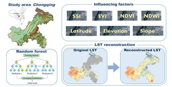
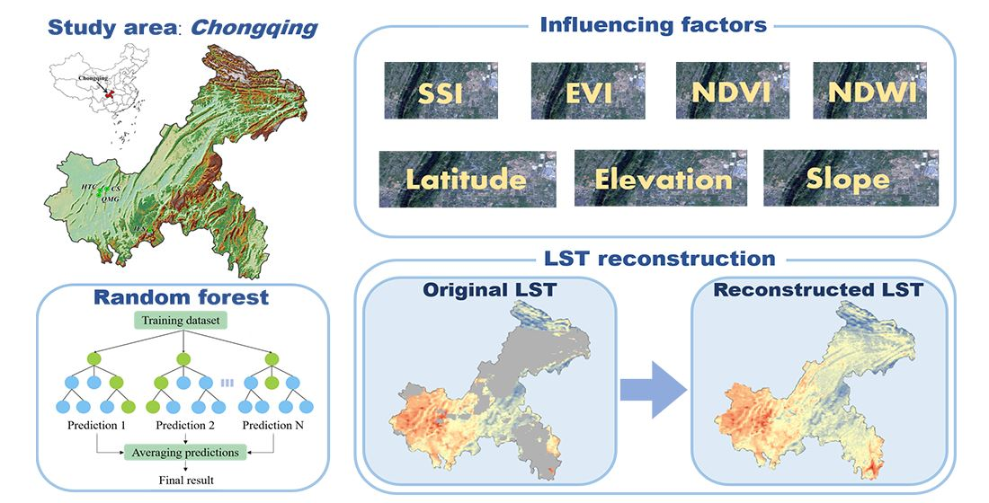
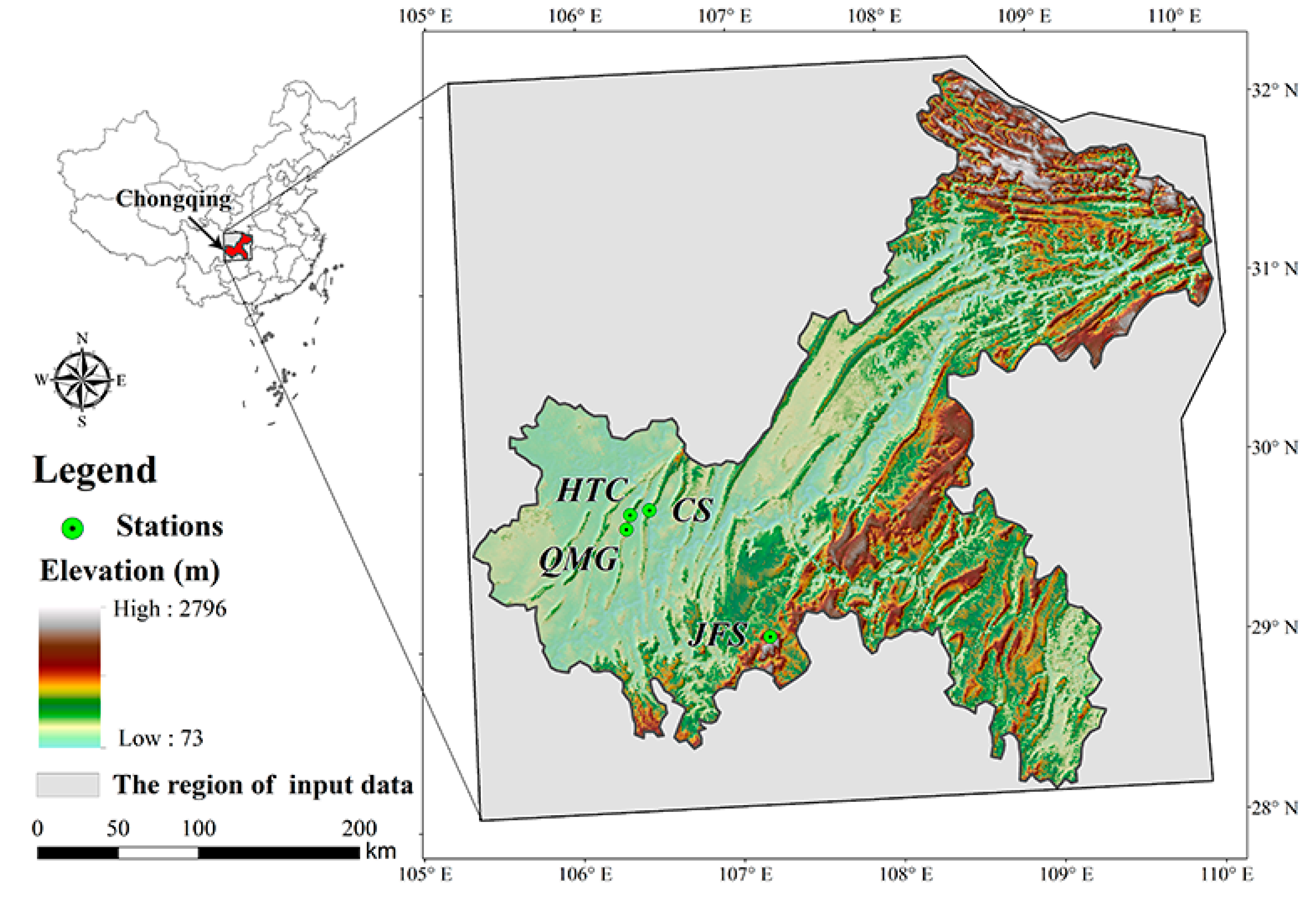
Here, a time-series LST product was generated based on the RF method, and an evaluation study was conducted in this study to further evaluate the performance of the reconstruction model. The Chongqing city in southwest China was selected as the study area and the in situ LST measurements from four sites, including Caoshang (CS), Hutoucun (HTC), Jinfoshan (JFS) and Qingmuguan (QMG), in this region were used to validate the reconstructed LST.
2. Materials and Methods
2.1. Study Area
Chongqing is located in southwest China, between 105°11′–110°11′ E and 28°10′–32°13′ N (Figure 1). The climate is subtropical humid, with a mean annual rainfall of 1240.9 mm and an average annual temperature of 14.6–15.6 °C. It has complex topographic features with elevation changing from 73 to 2796 m. The western Chongqing is located in the Sichuan Basin, and the east gradually uplifts eastward. As an inland city, Chongqing is characterized by its cloudy and foggy weather. The statistics based on MODIS daily observations in 2018 indicate that the number of the days with valid values for each pixel in this region accounts for 38 to 135. Therefore, it is a good place to evaluate the LST reconstruction study. To obtain more valid pixels for modeling, the study area was extended to cover the whole Chongqing city as shown in Figure 1.
2.2. Methodology and Data
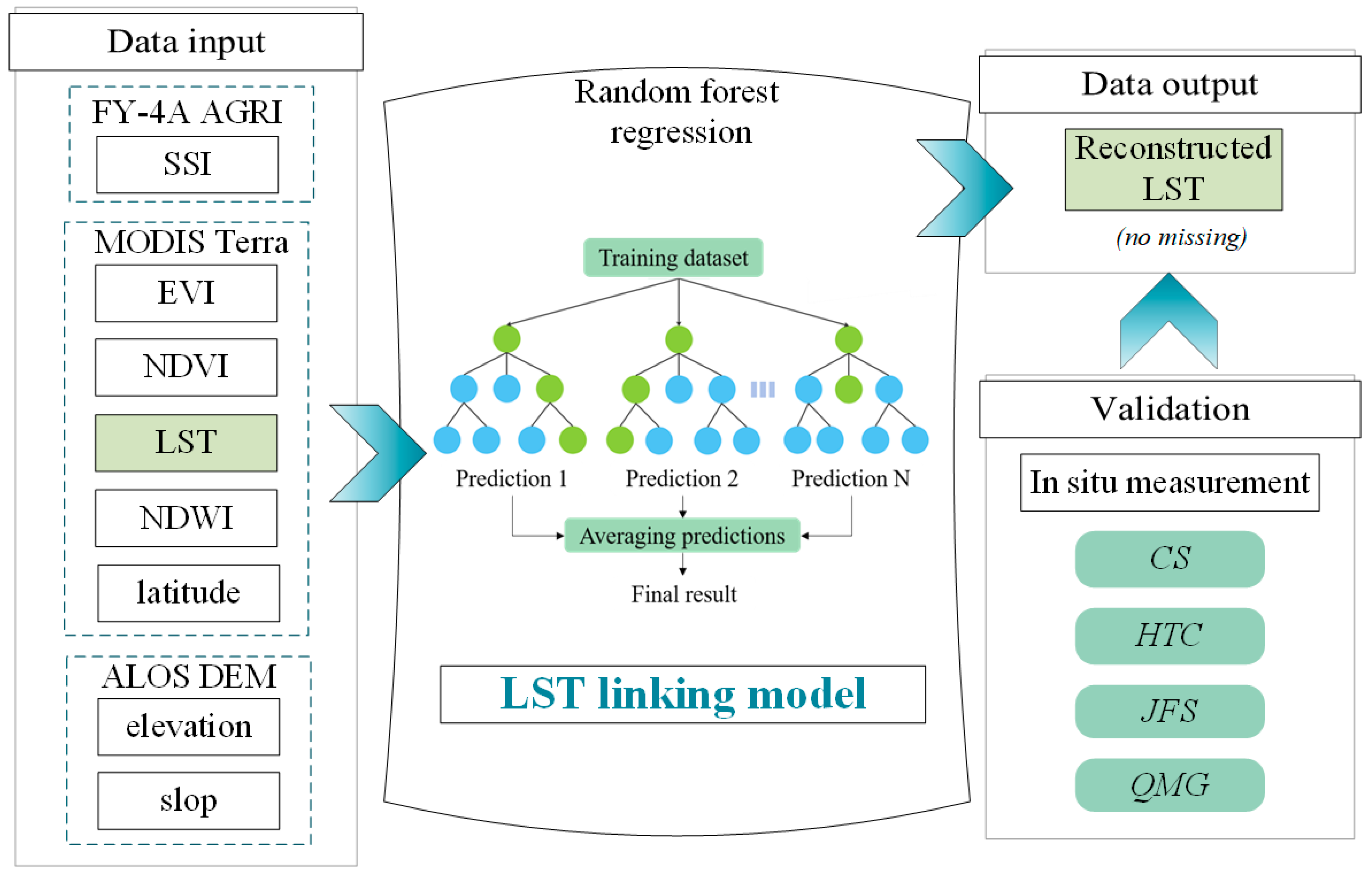
2.2.1. Random Forest-Based Reconstruction Model
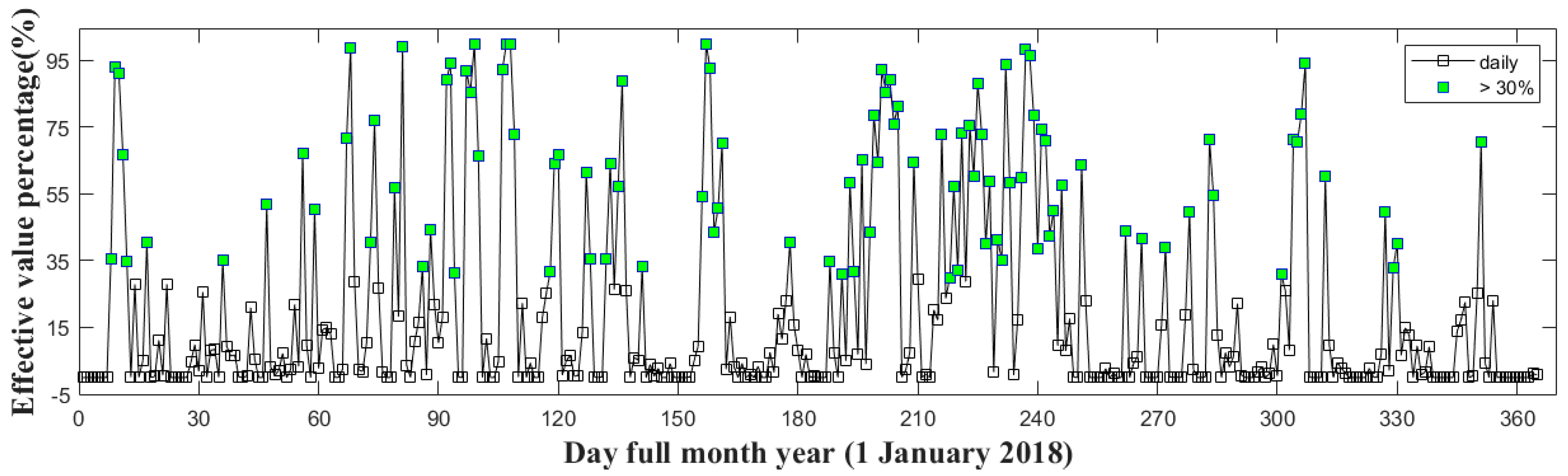
LST is impacted by incident surface radiation, topography, meteorology, land cover, latitude and elevation. Under cloud cover conditions, the incident solar radiation is blocked by cloud cover, which influences the evolution of LST in obscured areas. To effectively express the influence of environmental variables on effective LST, Zhao, et al. [30] constructed a LST linking model. Based on this LST linking model, Zhao and Duan [29] proposed a RF-based approach to reconstruct LST under the cloud cover. Compared with other reconstruction methods, this method is relatively independent from in situ measurements and shows high flexibility due to the large number of decision trees generated by splitting at each tree node by the random selection of a subset of training samples and a subset of variables. The predictors are NDVI (), EVI (), NDWI (), albedo (), elevation (), slope (), latitude () and solar radiation factor (). is estimated based on the cumulative value of surface solar irradiance between sunrise and the satellite overpass time. In this study, because the surface albedo product was strongly contaminated by frequent cloud cover in this region, a slight improvement was introduced in the reconstruction method of this study by excluding from the reconstruction process to avoid the impacts of cloud cover. The detailed flowchart of the reconstruction process was shown in Figure 2. The RF-based approach was firstly used to establish the LST linking model with the observations from clear-sky pixels. Then, the established linking model was applied to the cloud-covered pixels to estimate the actual LST values. During the estimation process, there should be enough clear-sky pixels available for the linking model construction to effectively capture the complex relationship between LST and these predictor variables. After many tests, a threshold of 30% of clear sky pixels are needed to determine whether the training samples are appropriate to reconstruct the LSTs under cloud cover. For days with less than 30% valid LST pixels, the reconstruction will not be conducted on these days. As shown in Figure 3, the number of the days passing the above requirement is only 102 in 2018. Before fitting the model, two important parameters need to be specified: The number of variables to be selected at each split (mtry) and the total number of trees to be grown (ntree). In this study, the machine learning library (Scikit-Learn 0.24.2) was used to build the link model in Python 3.8 (https://www.python.org/downloads/release/python-380/, accessed on 1 June 2021), and the ntree and mtry values were 500 and 3, respectively, which were selected based on several tests.
Finally, the in situ LST measurements acquired from the longwave radiation observations at four stations were used to validate the recovered LST and evaluate the reconstruction method.
2.2.2. MODIS Products
In this study, we selected the 1 km MOD11A1 product to implement the reconstruction of LSTs. The cloudy and low-accuracy pixels, with error larger than 1K, were removed according to the data quality control flags. Then the 3σ-edit rule, a widely used method for outlier detection [31], was used to remove outliers to obtain robust statistics for LST validation.
The surface reflectance data and the vegetation indices data were selected from MOD09A1 and MOD13A2 products, respectively, in this study. NDWI was calculated based on MOD09 A1 products. NDVI and EVI were available from MOD13A2 products. These datasets were used as related impact factor data to deduce the interrelationship between LST and its variables. The quality of vegetation indices is affected by various factors, such as the noise of anisotropic reflectance, electronic unstable errors, artificial data resampling and atmospheric condition. To reduce the noise induced by clouds, a temporal filter method, the Savitzky–Golay filtering (SG) technique [32,33], was used to smooth vegetation indices (NDVI and EVI) time-series products before running the RF-based reconstruction model. For the SG method, Lara and Gandini [32] have evaluated its performance and found that it showed more reliable results than other smoothing functions on a complex and heterogeneous landscape. All the MODIS datasets are downloaded from NASA’s Earthdata website (https://search.earthdata.nasa.gov/, accessed on 20 August 2020) for free.
2.2.3. Topographic Parameters
To obtain the terrain information, the freely available Advanced Land Observing Satellite (ALOS) 30-m DEM data was downloaded from the website (https://www.eorc.jaxa.jp/ALOS/en/aw3d30/, accessed on 20 August 2020). According to the DEM data, surface slope and elevation are calculated to be the terrain factors in the reconstruction process, and they were aggregated into 1 km matching the MODIS LST data using the bilinear interpolation method.
2.2.4. Solar Radiation Factor Estimation
represents the cumulative value of surface solar radiation from sunrise to satellite observing time. For pixels with permanent cloud cover, the value should be very small and its value will show a general increasing trend with the increase of the clear-sky duration. Therefore, it can represent the impact of cloud cover during the diurnal warming process. Regarding the advantage of high-temporal-resolution, FY-4A L2 Surface Solar Irradiance (SSI) data was selected in this study. FY-4A was launched on 11 December 2016. It is equipped with an advanced geosynchronous radiation imager (AGRI), which can provide a high-temporal-resolution (60-min) and a coarse-resolution (4-km) SSI product. SSI product was downloaded for free from the FENGYUN Satellite Data Center (http://data.nsmc.org.cn, accessed on 1 June 2021). To match the spatial resolution of the MODIS LST data, the FY-4A SSI product was interpolated to 1 km using a bilinear interpolation method. After this, the values were estimated by integrating the instantaneous data from sunrise to satellite observing time.
2.2.5. Validation Data
Four sites (shown in Figure 1) provide the in situ LST data estimated by the longwave radiation data to validate the reconstruction results. Before validation, it is necessary to verify that the in situ (point) datasets are representative on the satellite pixel scale [31]. Here the 90-m ASTER LST product downloaded from the website (https://search.earthdata.nasa.gov/, accessed on 15 January 2021) was selected to assess the spatial homogeneity of these stations.
Based on the thermal radiation transfer function, the in situ LST measurements can be estimated by the following function [34]:
where is the surface upwelling longwave radiation; is the surface downwelling longwave radiation; is the surface broadband emissivity; is the Stefan–Boltzmann constant (5.67 × 10⁻⁸ Wm−2 K−4); and is the in situ LST value. From this, can be estimated through the following form [35]:
where , and are the surface narrow-band emissivities of MODIS bands 29 (8.3 μm), 31 (10.8 μm) and 32 (12.1 μm), respectively, which are available from MOD11C1 monthly dataset.
3. Results
3.1. Visual Assessment for the Reconstruction LST
3.1.1. Original LST
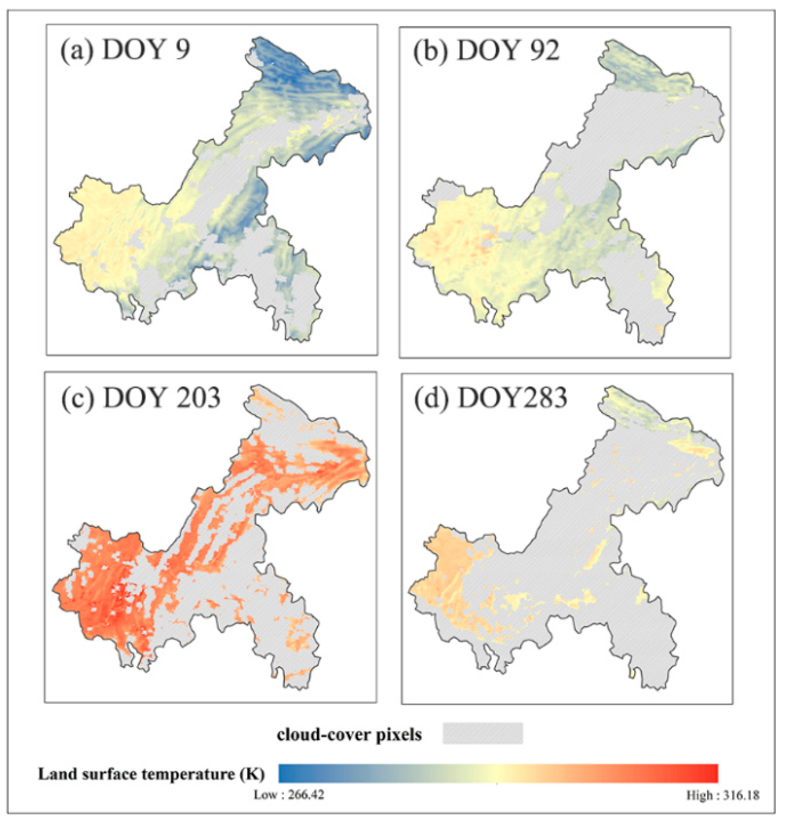
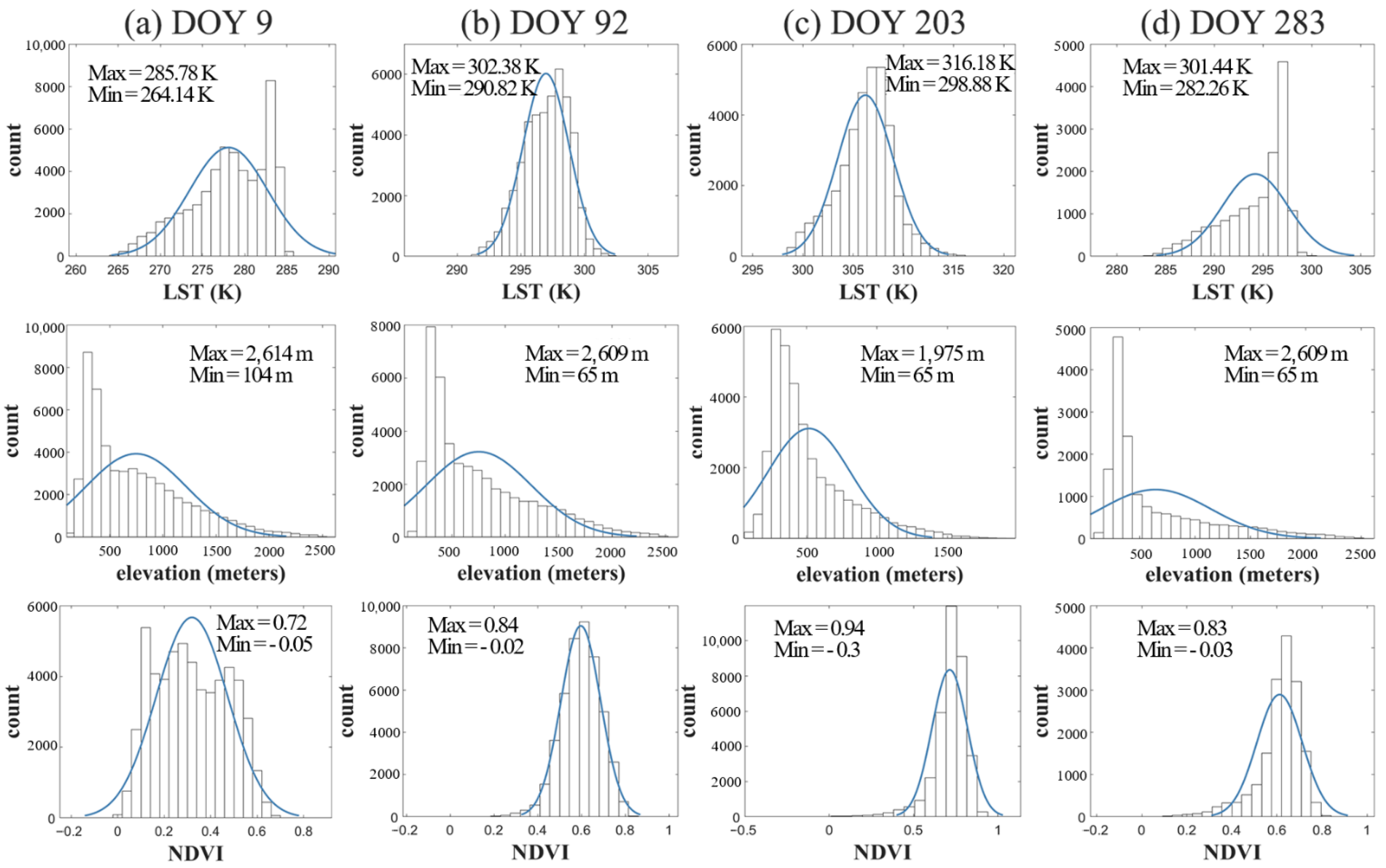
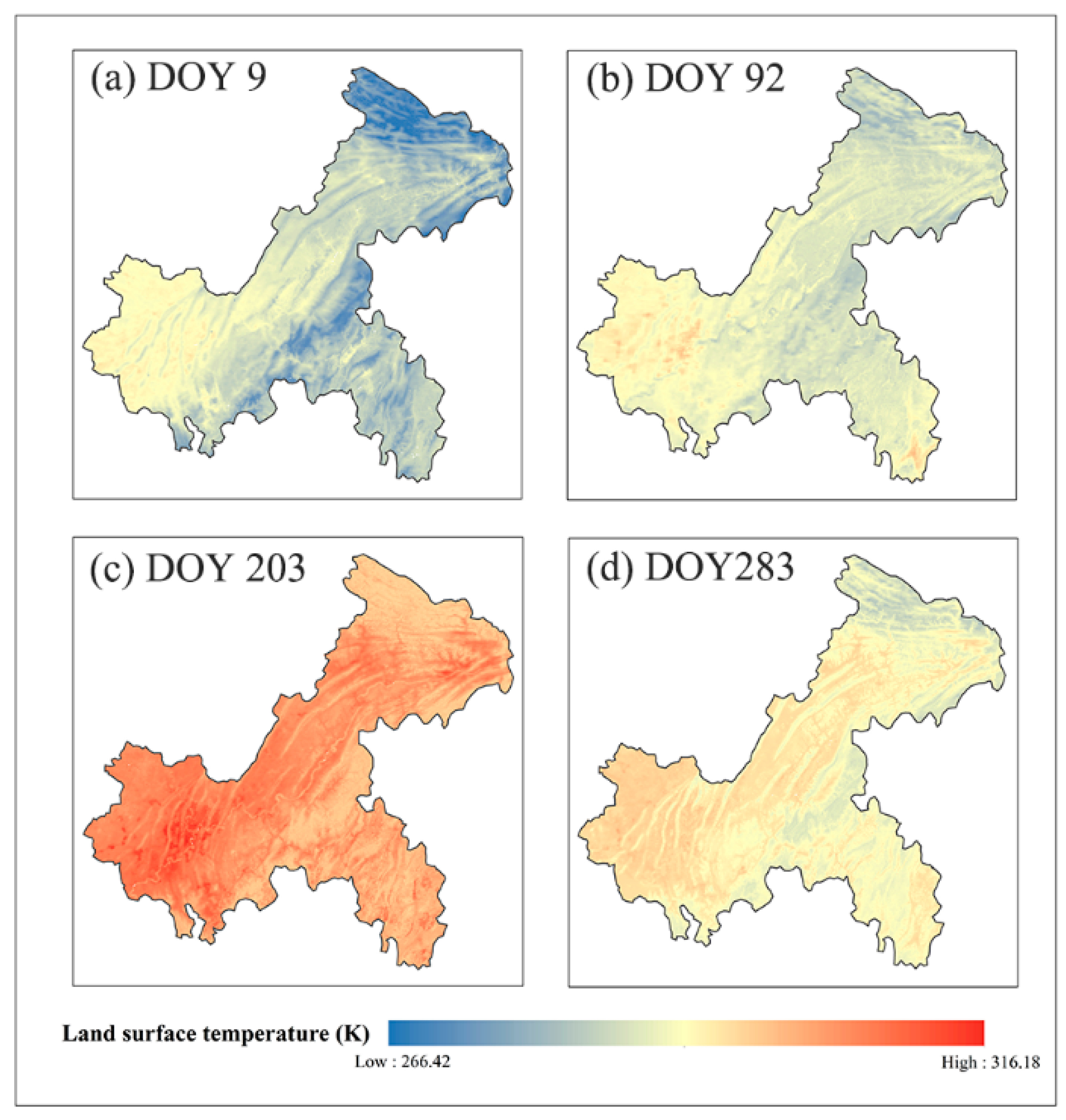
To present the reconstruction effect, four scenes at different seasons (the day of the year (DOY) 9, 92, 203 and 283 in 2018) were selected as examples. As shown in Figure 4, (DOY) 9, 92, 203 and 283 represented the winter, spring, summer and fall of the year, respectively. The data missing from these four days is serious, and the percentage of valid value in these images is 66.6%, 55.7%, 44.4% and 20.3%, respectively, and the pixels without data are mainly distributed in the northeast and southeast of Chongqing. The significant LST difference of these days can represent the distribution characteristics in one year, hence the reason for choosing these four days. The histogram profile of LST, elevation and NDVI on these four days is shown in Figure 5. The clear-sky pixels are distributed in both high elevation and high NDVI regions, as well as low latitude and low NDVI regions, that can describe the altitudinal and environmental temperature features and capture the characteristics of predictor variables. The input data including low LST and high LST pixels in a single day is beneficial to derive the complex relationships between LST and the variables. In addition, the size of pixels with value in four days is different, which can further demonstrate the impact of different sizes of input data on the accuracy of model construction.
3.1.2. The Impact of Cloud
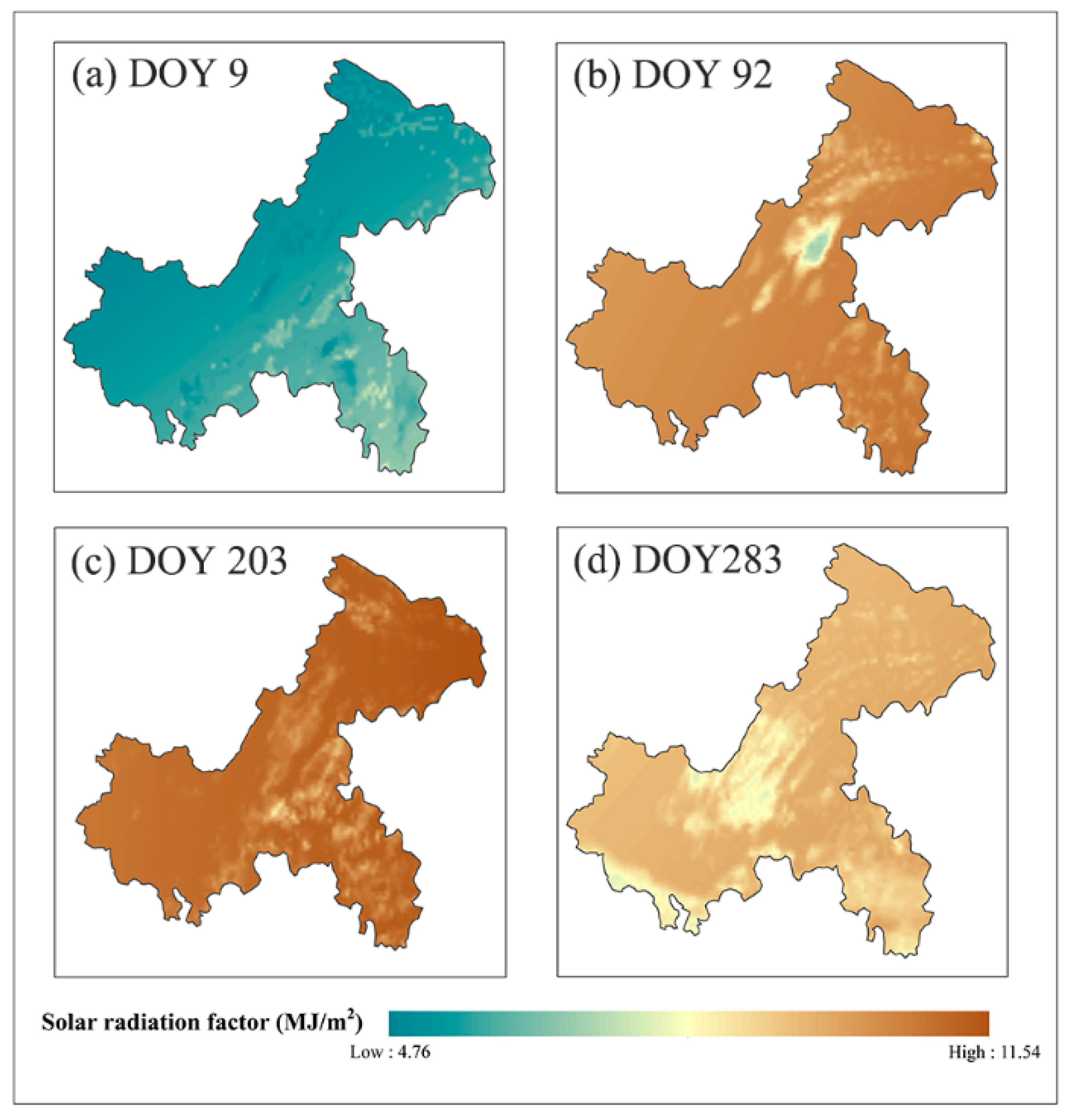
Along with the model fitting, clouds play an important role. Figure 6 shows the cumulative value of surface solar irradiance of these four days, which can present the impact of the cloud cover on solar radiation during the surface warming process. Comparing the cumulative SSI (Figure 6) with the original LST (Figure 4), the low value pixels of SSI and the blank areas of LST obscured by clouds have a similar spatial distribution. The mountains in the northeast and southwest are frequently covered by clouds that the cumulative SSIs are usually low. The cumulative SSI can account for the influence of cloud cover with different duration times. Therefore, based on the time-series FY-4A SSI product, the impact from different solar radiation conditions can be accurately monitored. Accordingly, the RF model effectively obtained the relationship between the LST and different surface variables, especially cloudy information.
3.1.3. Reconstructed LST
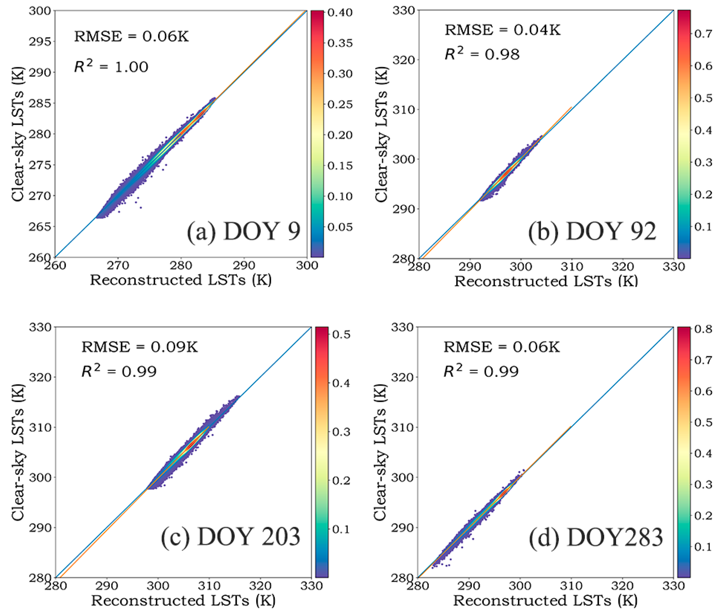
As shown in Figure 7, the density plots between the recovered LSTs and the valid LSTs illustrate the good performance of the LST linking model fitting. The coefficient of determination (R2) is above 0.98 and the root mean squared error (RMSE) is lower than 0.1 K; this demonstrates that the RF model maintains a relatively stable performance for different seasons with close agreement between the untrained LST values and the reconstructed LST values. Meanwhile, the input dataset was randomly divided into the training part and test part, containing 90% and 10% of the dataset, which was applied for cross-validation. The average out-of-bag score was above 0.98, that indicated the fitted model well describes the interactions between LST and the predictor variables. Along with the model fitting, the average variable importance scores for each variable of the reconstructed days is shown in Table 1. The high score values of , and is 0.299, 0.209 and 0.148, respectively, which present the strong correlation with LST. As shown in Figure 8, the reconstructed LST images have strong spatial continuity without abrupt increase or decrease. According to the spatial distribution of the reconstructed LSTs in these four days, it can be found that there is a similar increasing trend of LSTs from north to south. The LST variation associated with surface elevation can be clearly detected in all four images. The high elevation regions in the north and middle part of the study area usually have low LST, while the low elevation regions in the west part have high LST. Based this method, the reconstructed LST images clearly show the impact from the mountain ranges in the middle and western part of this region.
3.2. Validation of the Reconstructed LSTs
3.2.1. Evaluation of the Spatial Representativeness of In Situ LST Observations
Prior to the validation of the reconstructed LSTs, the spatial standard deviation (STD) of LSTs was calculated using a subset of 11 × 11 ASTER pixels corresponding to the MODIS pixel centered on each site [31]. The STDs of HTC and JFS sites are considerably larger than that of the other two sites shown in Table 2. However, all sites have a spatial STD lower than 1.7 K; therefore, they can be considered relatively homogeneous and can be used to directly validate the LSTs at MODIS scale.
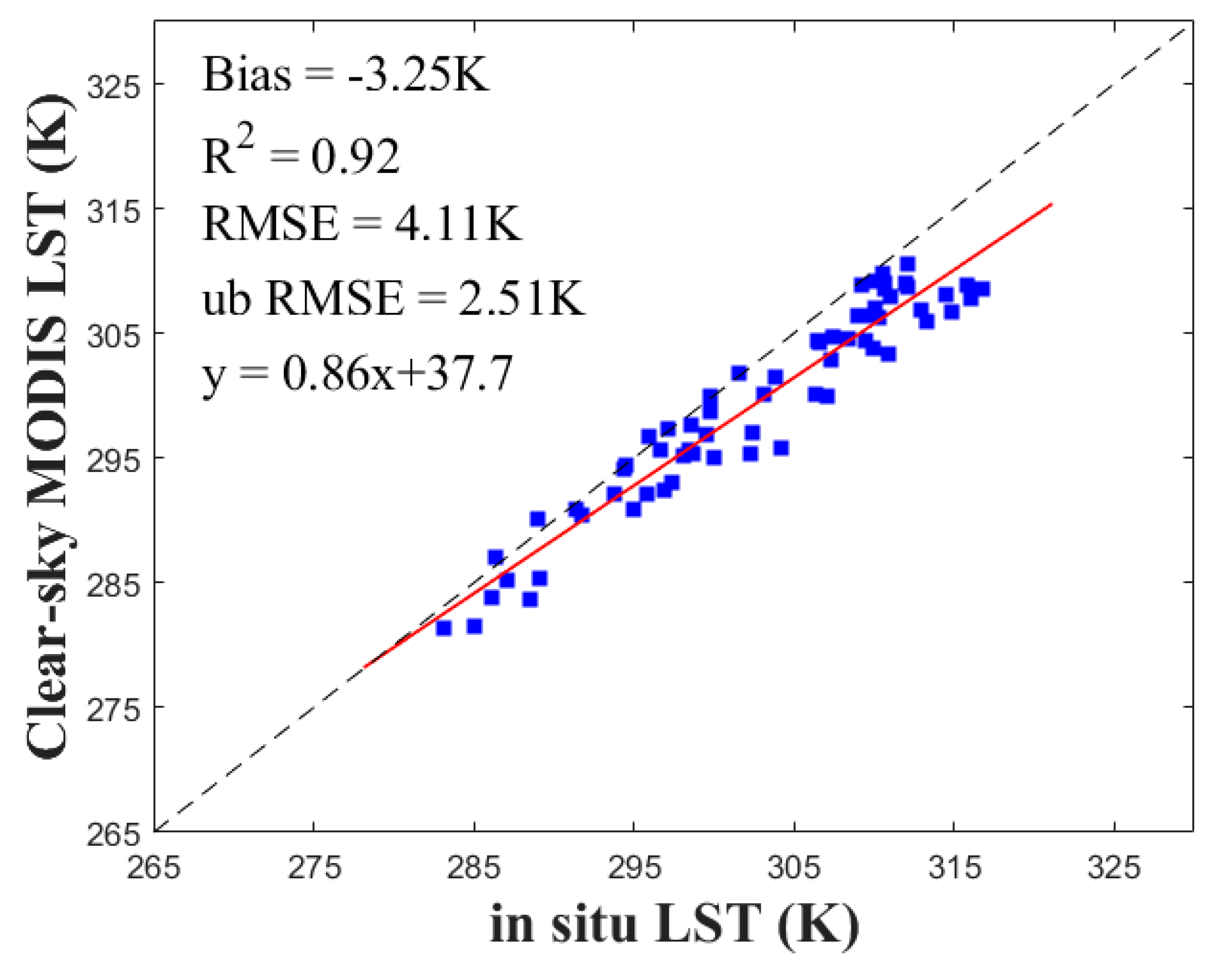
Meanwhile, the measurements from these sites were selected to assess the accuracy of the original MODIS LST product. The scatter plot shown in Figure 9 indicates that there is good correlation between two datasets with the R2 of 0.92 and the unbiased root mean squared error (ub RMSE) less than 3 K. However, there is a systematic negative bias in the MODIS LST product.
3.2.2. Validation with In Situ measurements
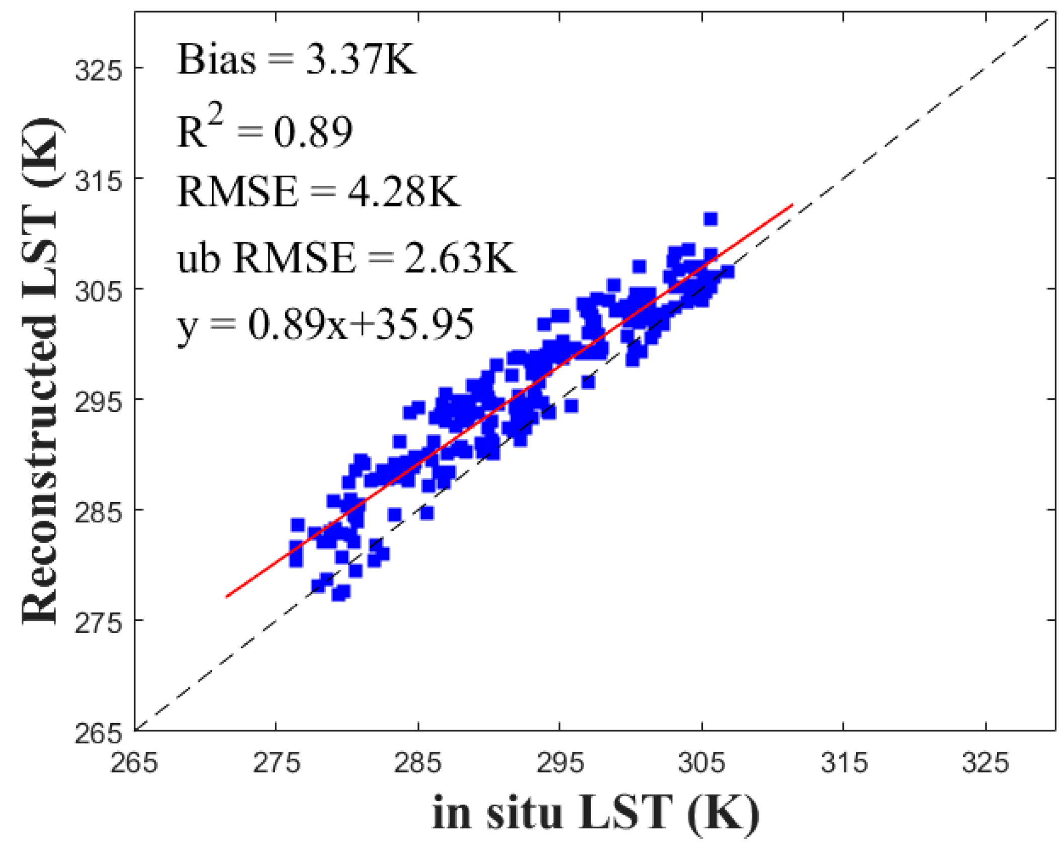
Figure 10 shows the reconstructed LSTs versus in situ measurements of four sites after removing the systematic biases. The scatter plot generally shows that the reconstructed LSTs at these four sites have a good correlation with the in situ data with an R2 value of 0.89 and the ubRMSE of 2.63 K. Additionally, most of the reconstructed LST values are concentrated near the 1:1 line, which demonstrates that the reconstructed LSTs have a good agreement with the original LSTs, and this method provides a reliable, robust filling result. Although the R2 is slightly lower than the comparison for cloud-free LST pixels, the bias is a little smaller according to the absolute value.
To further analyze the validation effects at different sites, the accuracy of the reconstructed LSTs was evaluated separately with in situ measurements at each site. Table 3 summarizes the statistics of these comparisons. For these four sites, the bias varies from 3.00 K to 4.87 K, meaning that a slightly systematic overestimation happens at all sites. The comparison results indicated that the validation at the JFS site is worse than other sites, especially in terms of bias. Combined with the STDs of four sites shown in Table 2, one possible reason for the significant discrepancies is spatial heterogeneity of LST at this site. Furthermore, the comparison results display that although some sites show a relatively large bias, the overall results generally present the strong correlation between two original LSTs and in situ LSTs. Therefore, we can conclude that the RF-based approach has satisfactory performance in reconstructing the LSTs under cloud cover.
4. Discussion
In this study, a RF-based approach was used restore the missing LST values affected by clouds. Although a visual comparison and ground-based measurements show satisfactory performance, there are various advantages and disadvantages in this research.
According to the statistics in 2018, there were only 38 to 135 days with valid values for each pixel in the study area. While this study area is continually and widely covered by clouds, it has complex terrain features. Therefore, the MODIS LST products are hardly available, which severely impedes regional research such as climate change assessments, agricultural drought monitoring and urban heat monitoring. In this paper, the RF approach performs well in reconstructing missing LST values in such a complex area. As Figure 8 shows, there is no extreme overestimation or underestimation in reconstructed LST and the cloud cover pixels were effectively filled. Meanwhile, the experimental results also infer that the RF approach is effective in reconstructing the missing values.
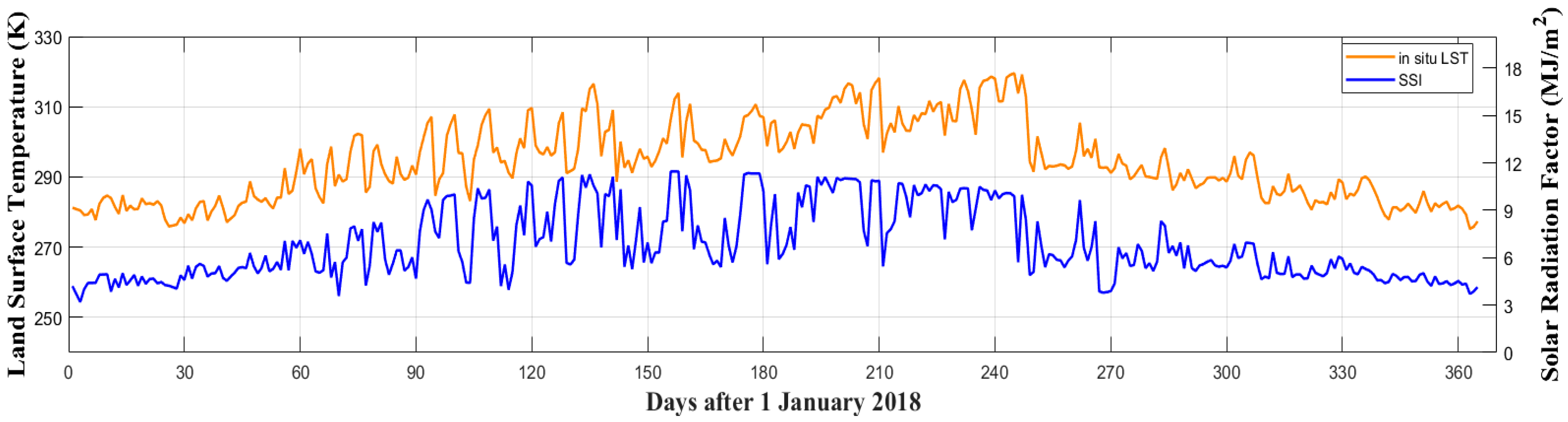
Zhao and Duan [29] used the Meteosat Second Generation (MSG) downward surface shortwave flux product to depict the impact of cloud cover on LST. Here, the FY-4A SSI product was selected to estimate the cumulative downward surface solar irradiance during the surface warming process. FY-4A is the first Chinese next-generation geostationary meteorological satellite. It was launched in 2016 and began operating in 2018. A comparison obviously displays that the spatial distribution of the invalid LST (Figure 4) from MODIS suffering from cloud cover is highly consistent in low value areas of the cumulative SSI images (Figure 6). Besides, Figure 11 shows a comparison of the in situ LST (orange curve) and the cumulative value of SSI (blue curve) with the day of the year. As shown in the Figure 11, these two curves exhibit good coherence and change similarly, which could suggest that the cumulative value of SSI sufficiently captured the impact of cloud cover on LST. Therefore, based on the FY-4A SSI product, the cloud-covered information of MODIS LST values between sunrise and satellite overpass time can be accurately estimated. can be obtained by the FY-4A SSI product, and the RF approach can be applied to the entire hemisphere’s LSTs with a longitude centered at 104°42′ E, theoretically. Compared with other methods [34,36], this reconstruction method is much more practical and independent, with the auxiliary data obtained from the FY-4A SSI product to describe the change of LST impacted by the cloud-covered conditions.
Despite the good performance of the result with the RF approach, some limitations still exist. First, the performance of the RF model depends on a sufficiently large data sample. Therefore, as many valid pixels as possible should be selected to fit the model. Based on empirical assumption, a cloud-free fraction of at least 30% is needed for the reconstruction studies in this study. To select abundant valid pixels to train the model, the data input used here covers the entire study area. Moreover, the fitted model has some inherent uncertainty associated with input datasets. For instance, the vegetation indices are smoothed by the SG filter, which leads to uncertainty in describing the actual surface circumstance for one specific day. To reduce the uncertainty of variables, the quality and error of datasets should be controlled before reconstruction.
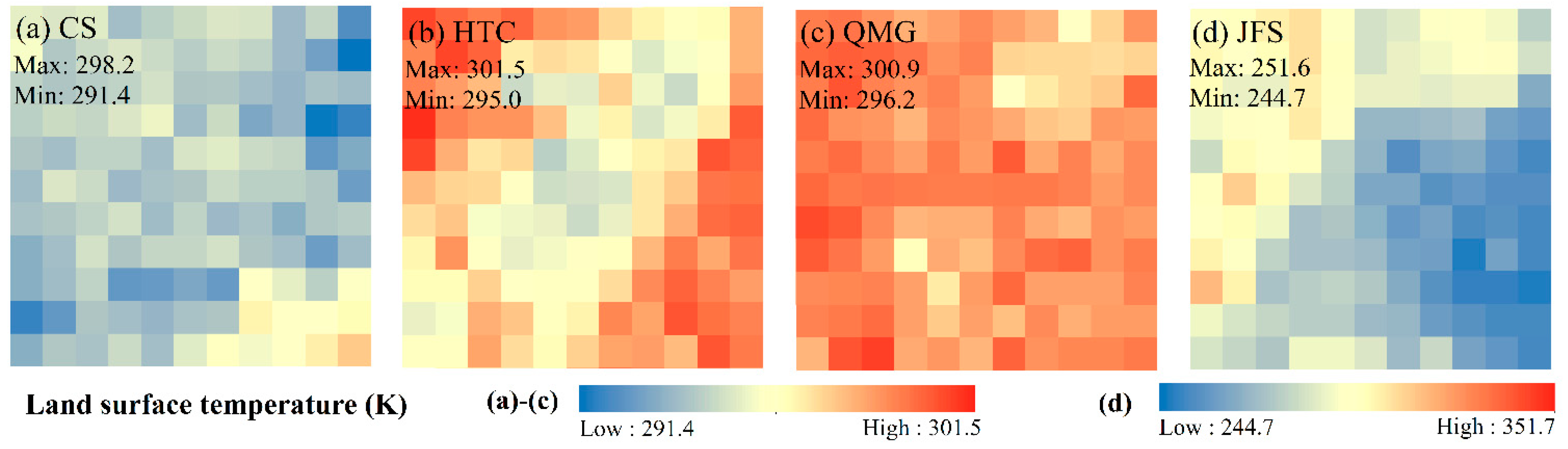
Second, there are many challenges in validation. Due to the limited availability of ground-based observations, there is a lack of abundant sites and measurements at a complete time-series for validation in the complex area. Moreover, because of the special spatial position in this region, the LST products reconstructed by this method are not compared with other reconstructed LST products [34,37]. Additionally, it is difficult to validate the LST products in such a heterogeneous region. As shown in Figure 12, a set of ASTER pixels (corresponding to the MODIS pixel) centered on each site (marked in Figure 1) were acquired in CS, HTC and QMG on 14 August and in JFS on 2 January under a clear-sky condition. Figure 12 indicates that for four sites in diurnal LST experiments, the LSTs in QMG demonstrate weaker heterogeneous structural characteristics than the other sites, whose LST difference at one MODIS LST pixel with a temperature of ~10K. Associated with the STDs of four sites shown as Table 2, there are large spatial variations in LST over the sites, which is influenced by strong convection systems, such as strong wind, heavy precipitation and rapid transition among the air masses. Therefore, it is necessary to ensure spatial homogeneity of the satellite pixel and high-quality in situ measurements before validation.
5. Conclusions
This study presented an evaluation of time-series LST reconstruction products under the influence of cloud coverage, based on the RF method. The time-series FY-4A SSI product was selected to obtain the relationship between the LST and the cloud cover. Through visual assessment and direct validation with in situ LST data collected from four sites in the study area, this evaluation indicated that the reconstruction method can sufficiently capture the spatial and temporal variations of LST under different land surface conditions. The topographic influence was clearly presented in the reconstructed LSTs. Furthermore, the quantitative validation also showed that the reconstructed LSTs have good correlation with in situ LST measurements with the R2 of 0.89. In general, the evaluation study confirmed the reliability of the reconstruction method in estimating LST under cloud-covered conditions. However, the size of the training dataset has a direct influence on the model accuracy, and the validation suffers from the topographic impacts. Therefore, how to improve the accuracy of this reconstructed method and validation in complex region should be investigated in further study.
Author Contributions
Conceptualization, Y.X. and M.M.; methodology, W.Z.; validation, Y.X. and W.Z.; formal analysis, Y.X., W.Z. and K.H.; resources, M.M. and W.Z.; data curation, Y.X. and K.H.; writing—original draft preparation, Y.X.; writing—review and editing, W.Z. and K.H.; supervision, M.M. and W.Z.; funding acquisition, M.M. and W.Z. All authors have read and agreed to the published version of the manuscript.
Funding
This research was funded by the National Natural Science Foundation of China Project, grant number 41830648 and 41771453; National Major Projects on High-Resolution Earth Observation System, grant number 21-Y20B01-9001-19/22; The Sichuan Science and Technology Program, grant number 2020JDJQ0003; and the Graduate Scientific Research and Innovation Foundation of Chongqing, grant number CYS20108. The APC was funded by the National Natural Science Foundation of China Project, grant number 41830648.
Institutional Review Board Statement
Not applicable.
Informed Consent Statement
Not applicable.
Data Availability Statement
Not applicable.
Acknowledgments
This manuscript was supported by the National Natural Science Foundation of China Project under Grant 41830648 and 41771453; National Major Projects on High-Resolution Earth Observation System under Grant 21-Y20B01-9001-19/22; The Sichuan Science and Technology Program under Grant 2020JDJQ0003; and the Graduate Scientific Research and Innovation Foundation of Chongqing under Grant CYS20108.
Conflicts of Interest
The authors declare no conflict of interest.
References
- Caselles, V.J.S.; César, C. A physical model for interpreting the land surface temperature obtained by remote sensors over incomplete canopies. Remote. Sens. Environ. 1992, 39, 203–211. [Google Scholar] [CrossRef]
- Li, Z.-L.; Tang, B.-H.; Wu, H.; Ren, H.; Yan, G.; Wan, Z.; Trigo, I.F.; Sobrino, J.A. Satellite-derived land surface temperature: Current status and perspectives. Remote Sens. Environ. 2013, 131, 14–37. [Google Scholar] [CrossRef] [Green Version]
- Jaber, S.M.; Abu-Allaban, M.M. MODIS-based land surface temperature for climate variability and change research: The tale of a typical semi-arid to arid environment. Eur. J. Remote Sens. 2020, 53, 81–90. [Google Scholar] [CrossRef]
- Zhao, W.; He, J.; Yin, G.; Wen, F.; Wu, H. Spatiotemporal Variability in Land Surface Temperature Over the Mountainous Region Affected by the 2008 Wenchuan Earthquake From 2000 to 2017. J. Geophys. Res. Atmos. 2019, 124, 1975–1991. [Google Scholar] [CrossRef]
- Lu, Y.; Wu, P.; Ma, X.; Yang, H.; Wu, Y. Monitoring Seasonal and Diurnal Surface Urban Heat Islands Variations Using Landsat-Scale Data in Hefei, China, 2000–2017. IEEE J. Sel. Top. Appl. Earth Obs. Remote. Sens. 2020, 13, 6410–6423. [Google Scholar] [CrossRef]
- Cui, Y.; Zeng, C.; Chen, X.; Fan, W.; Liu, H.; Liu, Y.; Xiong, W.; Sun, C.; Luo, Z. A New Fusion Algorithm for Simultaneously Improving Spatio-Temporal Continuity and Quality of Remotely Sensed Soil Moisture Over the Tibetan Plateau. IEEE J. Sel. Top. Appl. Earth Obs. Remote Sens. 2021, 14, 83–91. [Google Scholar] [CrossRef]
- Ren, M.; Pei, R.; Jiangtulu, B.; Chen, J.; Xue, T.; Shen, G.; Yuan, X.; Li, K.; Lan, C.; Chen, Z.; et al. Contribution of Temperature Increase to Restrain the Transmission of COVID-19. Innovation 2021, 2, 100071. [Google Scholar] [CrossRef]
- McMillin, L.M. Estimation of sea surface temperatures from two infrared window measurements with different absorption. J. Geophys. Res. 1975, 80, 5113–5117. [Google Scholar] [CrossRef]
- Soliman, A.; Duguay, C.; Saunders, W.; Hachem, S. Pan-Arctic Land Surface Temperature from MODIS and AATSR: Product Development and Intercomparison. Remote Sens. 2012, 4, 3833–3856. [Google Scholar] [CrossRef] [Green Version]
- Tomlinson, C.J.; Chapman, L.; Thornes, J.E.; Baker, C.J.; Prieto-Lopez, T. Comparing night-time satellite land surface temperature from MODIS and ground measured air temperature across a conurbation. Remote Sens. Lett. 2012, 3, 657–666. [Google Scholar] [CrossRef]
- Long, D.; Yan, L.; Bai, L.; Zhang, C.; Li, X.; Lei, H.; Yang, H.; Tian, F.; Zeng, C.; Meng, X.; et al. Generation of MODIS-like land surface temperatures under all-weather conditions based on a data fusion approach. Remote Sens. Environ. 2020, 246. [Google Scholar] [CrossRef]
- Zhang, X.; Zhou, J.; Liang, S.; Wang, D. A practical reanalysis data and thermal infrared remote sensing data merging (RTM) method for reconstruction of a 1-km all-weather land surface temperature. Remote Sens. Environ. 2021, 260. [Google Scholar] [CrossRef]
- Wan, Z.-M.; Dozier, J. A Generalized Split-Window Algorithm for Retrieving Land-Surface Temperature from Space. IEEE Trans. Geosci. Remote. Sens. 1996, 34, 892–905. [Google Scholar]
- Wan, Z.-M.; Zhang, Y.-L.; Zhang, Q.-C.; Li, Z.-L. Validation of the land-surface temperature products retrieved from Terra Moderate Resolution Imaging Spectroradiometer data. Remote Sens. Environ. 2002, 83, 163–180. [Google Scholar] [CrossRef]
- Duan, S.-B.; Li, Z.-L.; Leng, P. A framework for the retrieval of all-weather land surface temperature at a high spatial resolution from polar-orbiting thermal infrared and passive microwave data. Remote Sens. Environ. 2017, 195, 107–117. [Google Scholar] [CrossRef]
- Gerber, F.; Jong, R.d.; Schaepman, M.E.; Schaepman-Strub, G.; Furrer, R. Predicting Missing Values in Spatio-Temporal Remote Sensing Data. IEEE Trans. Geosci. Remote Sens. 2018, 56, 2841–2853. [Google Scholar] [CrossRef] [Green Version]
- Zeng, C.; Long, D.; Shen, H.; Wu, P.; Cui, Y.; Hong, Y. A two-step framework for reconstructing remotely sensed land surface temperatures contaminated by cloud. ISPRS J. Photogramm. Remote Sens. 2018, 141, 30–45. [Google Scholar] [CrossRef]
- Martins, J.P.A.; Trigo, I.F.; Ghilain, N.; Jimenez, C.; Göttsche, F.-M.; Ermida, S.L.; Olesen, F.-S.; Gellens-Meulenberghs, F.; Arboleda, A. An All-Weather Land Surface Temperature Product Based on MSG/SEVIRI Observations. Remote Sens. 2019, 11, 3044. [Google Scholar] [CrossRef] [Green Version]
- Zhang, X.; Zhou, J.; Göttsche, F.; Zhan, W.; Liu, S.; Cao, R. A Method Based on Temporal Component Decomposition for Estimating 1-km All-Weather Land Surface Temperature by Merging Satellite Thermal Infrared and Passive Microwave Observations. IEEE Trans. Geosci. Remote Sens. 2019, 57, 4670–4691. [Google Scholar] [CrossRef]
- Tan, J.; Che, T.; Wang, J.; Liang, J.; Zhang, Y.; Ren, Z. Reconstruction of the Daily MODIS Land Surface Temperature Product Using the Two-Step Improved Similar Pixels Method. Remote Sens. 2021, 13, 1671. [Google Scholar] [CrossRef]
- Lyon, S.W.; S⊘rensen, R.; Stendahl, J.; Seibert, J. Using landscape characteristics to define an adjusted distance metric for improving kriging interpolations. Int. J. Geogr. Inf. Sci. 2010, 24, 723–740. [Google Scholar] [CrossRef] [Green Version]
- Ke, L.; Ding, X.; Song, C. Reconstruction of Time-Series MODIS LST in Central Qinghai-Tibet Plateau Using Geostatistical Approach. IEEE Geosci. Remote. Sens. Lett. 2013, 10, 1602–1606. [Google Scholar] [CrossRef]
- Fan, X.-M.; Liu, H.-G.; Liu, G.-H.; Li, S.-B. Reconstruction of MODIS land-surface temperature in a flat terrain and fragmented landscape. Int. J. Remote Sens. 2014, 35, 7857–7877. [Google Scholar] [CrossRef]
- Hengl, T.; Heuvelink, G.B.M.; Perčec Tadić, M.; Pebesma, E.J. Spatio-temporal prediction of daily temperatures using time-series of MODIS LST images. Theor. Appl. Climatol. 2011, 107, 265–277. [Google Scholar] [CrossRef] [Green Version]
- Coops, N.C.; Duro, D.C.; Wulder, M.A.; Han, T. Estimating afternoon MODIS land surface temperatures (LST) based on morning MODIS overpass, location and elevation information. Int. J. Remote Sens. 2007, 28, 2391–2396. [Google Scholar] [CrossRef]
- Xu, Y.; Shen, Y. Reconstruction of the land surface temperature time series using harmonic analysis. Comput. Geosci. 2013, 61, 126–132. [Google Scholar] [CrossRef]
- Chen, Y.; Nan, Z.; Zhao, S.; Xu, Y. A Bayesian approach for interpolating clear-sky MODIS land surface temperatures on areas with extensive missing data. IEEE J. Sel. Top. Appl. Earth Obs. Remote Sens. 2020, 14, 515–528. [Google Scholar] [CrossRef]
- Kang, J.; Tan, J.; Jin, R.; Li, X.; Zhang, Y. Reconstruction of MODIS Land Surface Temperature Products Based on Multi-Temporal Information. Remote Sens. 2018, 10, 1112. [Google Scholar] [CrossRef] [Green Version]
- Zhao, W.; Duan, S.-B. Reconstruction of daytime land surface temperatures under cloud-covered conditions using integrated MODIS/Terra land products and MSG geostationary satellite data. Remote Sens. Environ. 2020, 247, 111931. [Google Scholar] [CrossRef]
- Zhao, W.; Duan, S.-B.; Li, A.; Yin, G. A practical method for reducing terrain effect on land surface temperature using random forest regression. Remote Sens. Environ. 2019, 221, 635–649. [Google Scholar] [CrossRef]
- Duan, S.-B.; Li, Z.-L.; Li, H.; Göttsche, F.-M.; Wu, H.; Zhao, W.; Leng, P.; Zhang, X.; Coll, C. Validation of Collection 6 MODIS land surface temperature product using in situ measurements. Remote Sens. Environ. 2019, 225, 16–29. [Google Scholar] [CrossRef] [Green Version]
- Lara, B.; Gandini, M. Assessing the performance of smoothing functions to estimate land surface phenology on temperate grassland. Int. J. Remote Sens. 2016, 37, 1801–1813. [Google Scholar] [CrossRef]
- Cai, Z.; Jönsson, P.; Jin, H.; Eklundh, L. Performance of Smoothing Methods for Reconstructing NDVI Time-Series and Estimating Vegetation Phenology from MODIS Data. Remote Sens. 2017, 9, 1271. [Google Scholar] [CrossRef] [Green Version]
- Yu, W.; Tan, J.; Ma, M.; Li, X.; She, X.; Song, Z. An Effective Similar-Pixel Reconstruction of the High-Frequency Cloud-Covered Areas of Southwest China. Remote Sens. 2019, 11, 336. [Google Scholar] [CrossRef] [Green Version]
- Wang, K.; Liang, S. Evaluation of ASTER and MODIS land surface temperature and emissivity products using long-term surface longwave radiation observations at SURFRAD sites. Remote Sens. Environ. 2009, 113, 1556–1565. [Google Scholar] [CrossRef]
- Liu, H.; Lu, N.; Jiang, H.; Qin, J.; Yao, L. Filling Gaps of Monthly Terra/MODIS Daytime Land Surface Temperature Using Discrete Cosine Transform Method. Remote Sens. 2020, 12, 361. [Google Scholar] [CrossRef] [Green Version]
- Zhou, J.; Liang, S.; Cheng, J.; Wang, Y.; Ma, J. The GLASS Land Surface Temperature Product. IEEE J. Sel. Top. Appl. Earth Obs. Remote Sens. 2019, 12, 493–507. [Google Scholar] [CrossRef]
Figure 1.
The location of the study area and location of validation stations.

Figure 2.
Flowchart of the LST reconstruction process for cloudy pixels.

Figure 3.
Percentage of MODIS LST pixels with valid values in the study area and their change with the day of the year.
Figure 3.
Percentage of MODIS LST pixels with valid values in the study area and their change with the day of the year.

Figure 4.
Original MODIS/Terra daytime LST images on four days in 2018 (DOY 9, DOY 92, DOY 203 and DOY 283).
Figure 4.
Original MODIS/Terra daytime LST images on four days in 2018 (DOY 9, DOY 92, DOY 203 and DOY 283).

Figure 5.
Histogram profiles of LST, elevation and NDVI on four days in 2018 (DOY 9, DOY 92, DOY 203 and DOY 283).
Figure 5.
Histogram profiles of LST, elevation and NDVI on four days in 2018 (DOY 9, DOY 92, DOY 203 and DOY 283).

Figure 6.
Estimated solar radiation factor on four days in 2018 (DOY 9, DOY 92, DOY 203 and DOY 283).
Figure 6.
Estimated solar radiation factor on four days in 2018 (DOY 9, DOY 92, DOY 203 and DOY 283).

Figure 7.
Model accuracy on four days in 2018 (DOY 9, DOY 92, DOY 203 and DOY 283).

Figure 8.
Reconstructed LST images on four days in 2018 (DOY 9, DOY 92, DOY 203 and DOY 283).

Figure 9.
Scatter plot of the clear-sky MODIS LST versus in situ measurements.

Figure 10.
Scatter plot of the reconstructed LST versus in situ measurements.

Figure 11.
The in situ LST and estimated solar radiation factor over the CS site and their change with the day of the year.
Figure 11.
The in situ LST and estimated solar radiation factor over the CS site and their change with the day of the year.

Figure 12.
ASTER LST images over the sites: (a–c) acquired on 14 August 2018 and (d) acquired on 2 January 2018.
Figure 12.
ASTER LST images over the sites: (a–c) acquired on 14 August 2018 and (d) acquired on 2 January 2018.


Table 1.
The average variable importance scores of the reconstructed days.
| 0.113 | 0.080 | 0.086 | 0.209 | 0.299 | 0.065 | 0.148 |
Table 2.
The spatial standard deviation (STD) of validation sites used in this study.
| Sites | CS | HTC | QMG | JFS |
|---|---|---|---|---|
| STD(K) | 1.03 | 1.59 | 0.78 | 1.62 |
Table 3.
Bias, R2, RMSE and ub RMSE of difference between the reconstructed LSTs and in situ for four sites.
Table 3.
Bias, R2, RMSE and ub RMSE of difference between the reconstructed LSTs and in situ for four sites.
| Sites | CS | HTC | QMG | JFS |
|---|---|---|---|---|
| Bias (K) | 3.00 | 3.61 | 3.05 | 4.87 |
| R2 | 0.88 | 0.90 | 0.88 | 0.68 |
| RMSE (K) | 4.11 | 4.32 | 3.78 | 5.79 |
| ub RMSE (K) | 2.81 | 2.38 | 2.24 | 3.13 |
Publisher’s Note: MDPI stays neutral with regard to jurisdictional claims in published maps and institutional affiliations. |
© 2021 by the authors. Licensee MDPI, Basel, Switzerland. This article is an open access article distributed under the terms and conditions of the Creative Commons Attribution (CC BY) license (https://creativecommons.org/licenses/by/4.0/).
Share and Cite
MDPI and ACS Style
Xiao, Y.; Zhao, W.; Ma, M.; He, K. Gap-Free LST Generation for MODIS/Terra LST Product Using a Random Forest-Based Reconstruction Method. Remote Sens. 2021, 13, 2828. https://0-doi-org.brum.beds.ac.uk/10.3390/rs13142828
AMA Style
Xiao Y, Zhao W, Ma M, He K. Gap-Free LST Generation for MODIS/Terra LST Product Using a Random Forest-Based Reconstruction Method. Remote Sensing. 2021; 13(14):2828. https://0-doi-org.brum.beds.ac.uk/10.3390/rs13142828
Chicago/Turabian StyleXiao, Yao, Wei Zhao, Mingguo Ma, and Kunlong He. 2021. "Gap-Free LST Generation for MODIS/Terra LST Product Using a Random Forest-Based Reconstruction Method" Remote Sensing 13, no. 14: 2828. https://0-doi-org.brum.beds.ac.uk/10.3390/rs13142828
Note that from the first issue of 2016, this journal uses article numbers instead of page numbers. See further details here.