
Hyperspectral and Multispectral Image Fusion Using Coupled Non-Negative Tucker Tensor Decomposition


1
Department of Electrical and Electronics Engineering, Shiraz University of Technology, Shiraz 13876-71557, Iran
2
Imec-Vision Lab, Department of Physics, University of Antwerp, 2610 Antwerp, Belgium
*
Author to whom correspondence should be addressed.
Remote Sens. 2021, 13(15), 2930; https://0-doi-org.brum.beds.ac.uk/10.3390/rs13152930
Submission received: 25 June 2021
/
Revised: 16 July 2021
/
Accepted: 21 July 2021
/
Published: 26 July 2021
(This article belongs to the Topic High-Resolution Earth Observation Systems, Technologies, and Applications)
Abstract
:Fusing a low spatial resolution hyperspectral image (HSI) with a high spatial resolution multispectral image (MSI), aiming to produce a super-resolution hyperspectral image, has recently attracted increasing research interest. In this paper, a novel approach based on coupled non-negative tensor decomposition is proposed. The proposed method performs a tucker tensor factorization of a low resolution hyperspectral image and a high resolution multispectral image under the constraint of non-negative tensor decomposition (NTD). The conventional matrix factorization methods essentially lose spatio-spectral structure information when stacking the 3D data structure of a hyperspectral image into a matrix form. Moreover, the spectral, spatial, or their joint structural features have to be imposed from the outside as a constraint to well pose the matrix factorization problem. The proposed method has the advantage of preserving the spatio-spectral structure of hyperspectral images. In this paper, the NTD is directly imposed on the coupled tensors of the HSI and MSI. Hence, the intrinsic spatio-spectral structure of the HSI is represented without loss, and spatial and spectral information can be interdependently exploited. Furthermore, multilinear interactions of different modes of the HSIs can be exactly modeled with the core tensor of the Tucker tensor decomposition. The proposed method is straightforward and easy to implement. Unlike other state-of-the-art approaches, the complexity of the proposed approach is linear with the size of the HSI cube. Experiments on two well-known datasets give promising results when compared with some recent methods from the literature.
1. Introduction
Hyperspectral imagery utilizes a broad range of the electromagnetic spectrum to obtain information of the imaged scene, allowing better identification of materials or detection of processes. As each band of a HSI contains the spectral response to a narrow interval of the electromagnetic spectrum, it is necessary to collect reflectance from a wider area on the scene, decreasing the spatial resolution of HSIs. HSI acquisition instruments have extensive limitations for capturing high-resolution images, and there is always a tradeoff between spectral resolution and spatial resolution.
Hence, we always need spatial information provided from outside; using an auxiliary image consisting of panchromatic image, multispectral image or an RGB one is a well-known approach. In recent years, there have been several attempts which fuse a high resolution multispectral image (HRMSI) with a low resolution hyperspectral image (LRHSI) [1,2,3,4,5,6,7,8,9,10,11,12,13] to produce a high spatio-spectral resolution HSI. Basically, all fusion approaches can be grouped in the following categories: methods using a Bayesian framework [6,11,14,15,16,17,18], matrix factorization based methods [4,5,12,19,20,21], tensor factorization based methods [1,3,9,22,23,24,25] and deep learning based methods [26,27,28].
Bayesian methods apply the observed LRHSI and HRMSI and some prior information or regularization terms to build up the statistical model for estimating a super-resolution HSI [29]. In [11], a Bayesian framework is introduced, based on a sparse representation along with the alternating direction method of multipliers (ADMM) to solve the fusion problem. In our previous work [15], smooth graph signal modeling is employed to regularize in order to incorporate the spatio-spectral joint structural features of the HSI. The method proposed in [6] uses spectral unmixing and sparse representations in a Bayesian framework to increase the spatial resolution of the HSI. The most important deficiency of the Bayesian framework is that regularization terms are required that should comprehensively represent spatial information of HSIs, which is partially lost by matricizing the HSI.
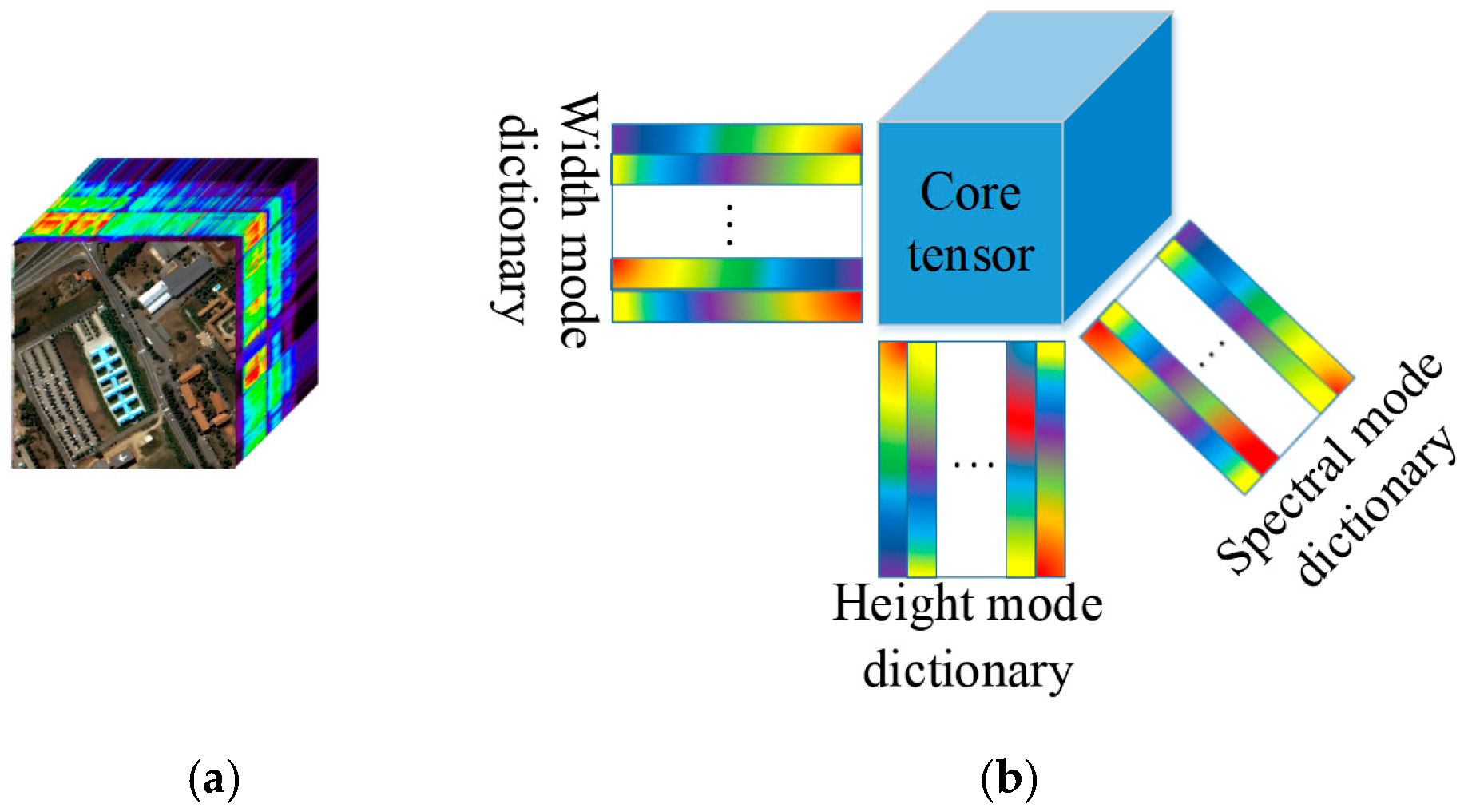
As an alternative approach, matrix factorization approaches have been widely applied to fuse LRHSI with HRMSI [4,5,12,19,20,21]. These methods describe the targeted high resolution HSI (HRHSI) as a product of a matrix of basis vectors of spectral signatures, learned from the high spectral resolution LRHSI, and a coefficient matrix, estimated from auxiliary data, such as a HRMSI. The method proposed in [4] exploits non-local self-similarity, based on a spatial and spectral sparse representation to estimate both basis vectors and coefficient matrices. Ref. [5] employed a non-negative structured sparse representation to estimate the spectral basis vectors, and a structured sparse representation is utilized to determine the coefficient matrices. In [19,20], the spatial structure of HRHSI is applied as regularization to estimate the super-resolution HSI. The method proposed in [12] applied spectral unmixing to regularize the fusion problem. This method alternately updates spectral basis vectors and coefficient matrices, subject to non- negativity and sum-to-one constraints. As HSIs are essentially non-negative data, non-negative matrix factorization (NMF) frameworks are quite compatible with the observed data. Therefore, the approach proposed in [21] alternately factorizes the LRHSI and HRMSI under non-negativity constraints, and multiplicative update rules (MUR) [30] are engaged to estimate the two factorized matrices in each stage. Of note, in Bayesian frameworks and NMF-based approaches, the 3D data structure is stacked into a matrix form, which causes a loss in the neighborhood structures, smoothness, and continuity characteristics. To avoid this, tensors or multiway arrays have been frequently used in hyperspectral data analysis for the purposes of image classification [31,32,33], data compression [34,35], change detection [36,37], target and anomaly detection [36,38], and denoising [39,40]. Additionally, exploiting the capability of multilinear algebra on the multiway array representations allows more flexibility in choosing constraints and describing data structures. Moreover, more general features can be extracted from the data compared with the matrix-based approaches. More recently, tensor-based representations have been widely used for HSI super-resolution [1,9,22,24,41]. The representation of a HSI as a tensor of order three is a structural and natural model without any loss of information. In most of these methods, a low rank tensor representation is exploited to estimate the HRHSI. It offers the benefits of extreme noise and memory usage reduction, and extraction of discriminative features [41]. Accordingly, two well-known tensor decompositions, the Canonical Polyadic decomposition (CPD) and the Tucker decomposition, are frequently used to estimate HRHSIs [9,22,24,25,31,42]. The former decomposes a tensor into the sum of component rank-one tensors, while the later factors three-dimensional data into the multiplication (mode-n products) of four fractions: a core tensor and three dictionary matrices corresponding to each mode (see Figure 1). In [22], a low rank tensor-train representation is incorporated for HSI super-resolution. In [23], nonlocal sparse tensor factorization is proposed to model non-local self-similarity of HSIs. In [24], a nonlocal coupled CPD framework is used to fuse hyperspectral and multispectral images. A spatio-spectral sparsity prior constraint is imposed on the core tensor in a coupled sparse tensor factorization method in [9]. In [38], a low-rank constraint is applied to the core tensor in the Tucker representation to detect anomalies in HSI. It effectively shows the superposition of a spectral background and the anomaly signatures. A coupled CP decomposition based method is proposed in [43], which fused LRHSI and HRMSI to produce a HRHSI in a tensor framework. Note that the CP-based rank of a tensor is defined as the minimum of rank-one component tensors that are summed to express that tensor, which is unknown and generally not easy to estimate. Meanwhile, in the Tucker representation there is just one component tensor which is called the core tensor. It can comprehensively express the relations between the various modes and multilinear interactions among them.
Moreover, with the recent success of deep learning techniques in various image processing tasks, an increasing research interest arose for deep learning-based image fusion. In [27] a fusion method based on convolutional neural networks (CNN) was proposed, in which the two CNN branches are devoted to spectral features of the LR-HSI and spatial neighborhood features of the HR-MSI, respectively. In [28], an unsupervised deep approach was proposed for a blind fusion of HRMSI and LRHSI, considering no prior assumptions on spatial and spectral degradation functions. Instead, they are modeled with deep network structures. The largest deficiency of the deep learning-based methods is their requirement of huge amounts of training data, which is practically not available. Furthermore, deep learning-based methods have limited generalization ability regarding the different sensor characteristics such as spectral range and the observational models.
AS HSI is naturally non-negative data, it has a strong prior knowledge to apply to the tensor factorization method, which is expected to further improve the performance of the fusion. In this paper, we extend NMF to a tensor framework, applying a non-negative tensor decomposition. Contrary to the conventional NMF-based methods, where the spatial, spectral, or their joint structural features must be additionally imposed as constraints, in this paper, the spatio-spectral joint structures of HSIs are preserved without having to impose constraints. We optimally exploit the spectral properties of the LRHSI and the spatial properties of the HRMSI, by directly applying a coupled (non-negative) Tucker decomposition to both images. We will refer to the proposed method as coupled non-negative Tucker decomposition (CNTD).
Using the Tucker tensor representation, the proposed method comprehensively models multilinear modes of the HSI, where the core tensor precisely expresses the relations between the various modes. Therefore we proposed this tensor framework to benefit from its ability to preserve spatio-spectral joint structures. Regarding the huge amount of data in hyperspectral image processing and analysis, computation efficiency is a significant factor. Thus, we propose an algorithm which is straightforward and easy to implement, with a complexity, linear with the size of the hyperspectral data cube. The main contributions of this paper are highlighted below.
- The application of non-negativity priors to the Tucker tensor decomposition of LRHSI and HRMSI, to estimate spectral and spatial mode-dictionaries in a Tucker model, respectively. To the best of our knowledge, this is the first time that a non-negative Tucker decomposition is used to represent hyperspectral images in a HSI fusion framework.
- The preservation of spatio-spectral joint structures of HSIs without prior knowledge requirements and much lower information losses than matrix frameworks.
- The construction of an algorithm with lower-order complexity than the state-of-the-art.
The remainder of this paper is organized as follows. Some preliminaries on tensors are given in Section 2. Section 3 formulates the HSI-MSI fusion framework. The proposed coupled non-negative tensor decomposition (CNTD) method for super-resolution HSI is introduced in Section 4. The complexity of the proposed method is elaborated in Section 5. Section 6 describes some experimental results on two well-known datasets, Pavia University and Indian Pines. Finally, conclusions and future work are described in Section 7.
2. Preliminaries on Tensors
Let us denote a tensor of order N as , having N indices and its members by where . Tensor matricization unfolds a tensor of order N into a matrix. The mode- matricization of reorders the elements of to form the matrix . Tensor matricization can be regarded as an extension to matrix vectorization.
The mode-n product of tensor and matrix , is defined by , and entries are calculated by:
The mode-n product can also be denoted in matrix form as . The mode-n product has two important properties: (i) the order of multiple mode-n products with different modes is arbitrary:
and for multiple mode-n products with the same modes, the order is relevant:
The scalar product of two tensors indicated as . The Frobenius norm of a tensor is indicated as
The Tucker decomposition of is expressed as mode products of a core tensor and N mode matrices , which is expressed as:
which has an element-wise form given by:
The mode-n matricization form of is expressed by Kronecker products () of the mode-n matricization of the core tensor and mode matrices, as:
where is the mode-n matricization of the core tensor The Kronecker product of two matrices and is a matrix denoted by , defined as:
The following Kronecker product properties and the vectorization operation () are used in this paper:
All basic notations are presented in Table 1.
3. HSI-MSI Fusion Problem Formulation
In this paper, the HRHSI, LRHSI, and HRMSI are denoted as tensors of order three. The target HRHSI is denoted by , where , and are the width, height and number of spectral bands, respectively. The LRHSI and HRMSI are denoted by and , respectively, with ≪ , ≪ and ≪ . In this paper, we aim at estimating a HRHSI in a fusion framework, based on the observations and . In this section, we briefly describe the matrix factorization-based fusion scheme and then detail the tensor decomposition-based scheme.
3.1. Matrix Factorization-Based Fusion Scheme
In the matrix factorization-based fusion scheme, each spectral signature of the HRHSI is considered to be a linear mixture of a small number of basis vectors:
where, is the mode-three matricization of . contains the basis vectors in its columns and is the coefficient matrix. Similarly and are the mode-three matricization of and , respectively. Conventionally, they can be considered as spectral and spatial down-sampled versions of the target HRHSI. Thus:
where, is the point spread function (PSF) matrix and the spatial down-sampling in the hyperspectral sensor. It can be separated regarding width and height modes [9]:
where and are spatial separable down-sampling operators of the width and height spatial modes, respectively.
Similarly:
where is a matrix, modeling spectral down-sampling in the multispectral sensor. Therefore, the spectral response functions (SRF) of the multispectral sensor is included within its rows.
Commonly, in the HSI-MSI fusion problem formulation, the SRF and PSF are assumed to be known [4,9,11,17,25]. the proposed approach in [19] is also used to approximate the SRF and PSF from observed data. Following (10):
which, according to (12), can also be written as:
In, an optimization framework, based on quadratic regularizing, is presented to estimate and from the observed LRHSI and HRMSI:
where and are quadratic regularizers, and are the respective regularization parameters. See [19] for more details.
3.2. Tensor Decomposition-Based Fusion Scheme
As HSIs are naturally 3D data, the tensor is a more efficient representation than a matrix form, and we can benefit from its ability to exploit intrinsic structures of the HSI and multilinear interactions between its different modes. Hence, in this paper, the target HRHSI is formally expressed by:
which is called the Tucker representation, where , and are width, height and spectral dictionary matrices, respectively. , and are the number dictionary atoms of each mode, and is the core tensor that denotes the interactions between several modes.
Mode-n matricizations of are given by:
Similarly, both LRHSI and HRMSI are represented by:
where , and are width, height, and spectral dictionary matrices, respectively, and and denote Independent-Identically-Distributed (i.i.d.) noise of and , respectively. As the LRHSI and HRMSI are the spatially and spectrally down-sampled form of the HRHSI, respectively, one has:
4. Proposed CNTD Approach
The goal of a LRHSI and HRMSI fusion framework is to estimate a high spatio-spectral target HSI. Since , and , the super resolution problem is severely ill-posed and prior information is needed to regularize the fusion problem. Orthogonality and statistical independency of basis vectors in the Tucker representation, and sparsity, smoothness, and non-negativity of HSIs are some constraints that help to find a unique solution for the super-resolution problem of HSIs [44,45,46].
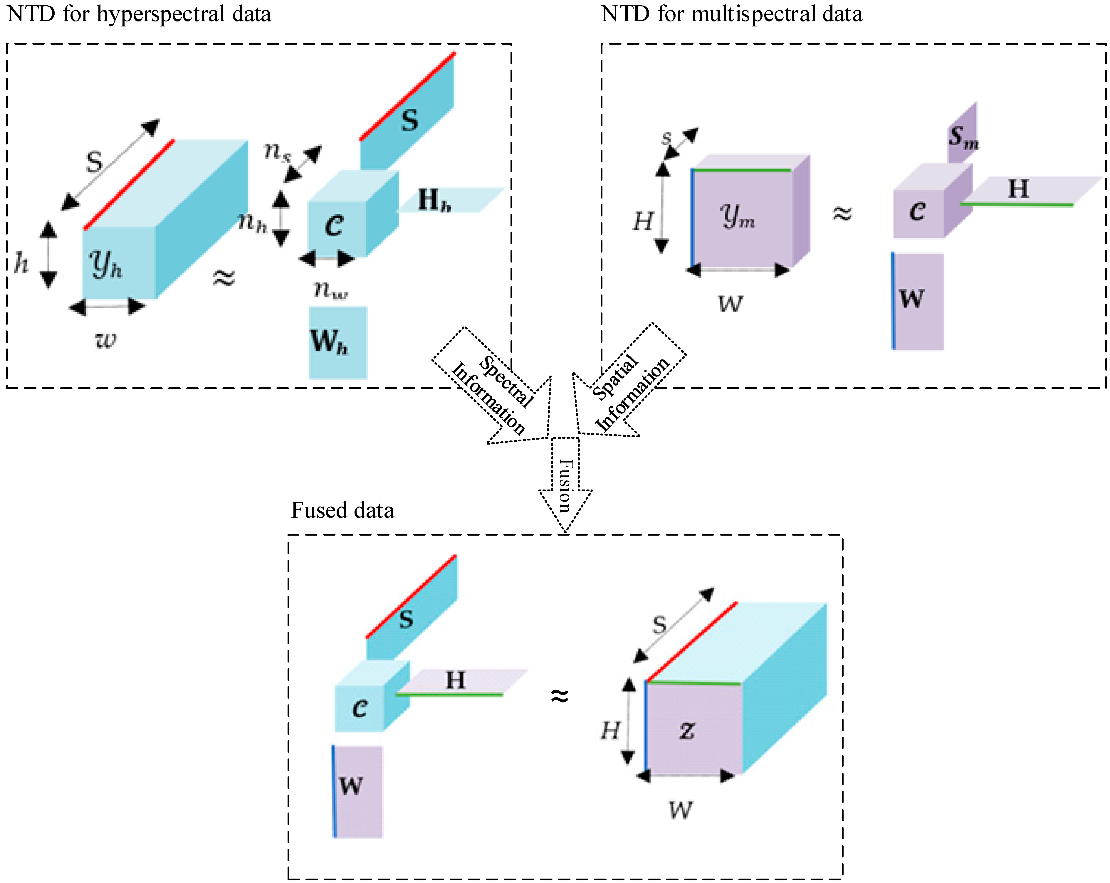
In this paper, we propose a new algorithm based on coupled non-negative Tucker decomposition (CNTD). The proposed method performs Tucker tensor decomposition of the LRHSI and HRMSI, subject to NTD. The original NMF method inherently loses spatio-spectral joint structure information when unfolding the 3D data into matrix form. Therefore, in this paper, we impose NTD to both tensors of the HSI and MSI directly. The CNTD method effectively combines multiple data tensors, where the intrinsic spatio-spectral joint structures of HSI can be represented without loss and interdependently exploited. The proposed CNTD approach is depicted in Figure 2, illustrating the fusion of the spatial information of HRMSI and the spectral information of LRHSI to produce the HRHSI.
Considering (16), (18), and (19), the LRHSI and HRMSI fusion problem is formulated by the following constrained least square optimization problems:
Hyperspectral and multispectral data fusion, based on NTD, is executed by the estimation of the corresponding dictionaries and the core tensor. The non-negative Tucker tensor decomposition is non-convex in its entirety, but it is convex in each of its factors. We easily derive updated rules for each mode-dictionary matrix by matricizing the Tucker model into its corresponding modes. Therefore, these can be considered as conventional NMF for which we use a block coordinate descent scheme. Therefore, the cost functions are optimized with respect to each factor while keeping the others fixed. Traditionally in gradient descent, the learning rates are positive, but since the subtraction of terms in the updated rules can lead to negative elements, Lee and Seung [30] proposed to use adaptive learning rates to avoid subtraction and thus the production of negative elements. Like the conventional NMF, the optimization algorithm is easy to implement and computationally efficient. NTD attempts to decompose a non-negative data tensor into the multilinear products of a non-negative core tensor and non-negative mode-dictionary matrices [47]. To minimize the predefined optimization problems (23) and (24), the multiplicative update rule (MUR) is applied, and can be directly achieved by NMF multiplicative rule, for which the convergence to local optima under the non-negativity constraints has been proven in [30,48].
4.1. Updating Mode-Dictionary Matrices
Updating algorithms for each mode-dictionary matrix can be easily derived by matricizing the Tucker model into its corresponding modes. Lee and Seung’s multiplicative update rule has been a widely known approach owing to the simplicity of its implementation [30]. We use an extended MUR for the mode-dictionary matrices of . The first mode matricization of is given by:
where and are the first mode matricization of LRHSI () and the core tensor (), respectively. Equation (25) can be rewritten as , just like the conventional NMF, for which the updating rules are given by [49]:
Equation (25) can be treated as the conventional NMF, where each fraction is updated using MUR (26):
where the fraction line denotes the element-wise division.
Similarly, the second mode matricization of is given by:
and the second mode-dictionary matrix is updated as:
Finally, the third mode matricization of is given by . Therefore, the spectral mode-dictionary () is updated as:
4.2. Updating Core Tensor
Applying (8) to (25):
which can be treated as the conventional NMF as well. Incorporating MUR to calculate the core tensor ():
Applying (8) to the numerator of (32):
and its denominator is given by:
As a result, the core tensor is updated by:
When performing MUR for in a similar way, the following updating relations for are obtained:
As the LRHSI and HRMSI contain, respectively, spectral and spatial information of the target image, the spectral mode-dictionary is initialized using the former and the spatial mode-dictionary matrices of the height H and width W are initialized using the latter. The spectral mode-dictionary is initialized using the simplex identification split augmented Lagrangian (SISAL) algorithm [50], which efficiently identifies a minimum volume simplex containing the LRHSI spectral vectors. The spatial mode-dictionary matrices W and H are initialized from the mode-one and -two matricization of the HRMSI, respectively, via dictionary update cycles of the KSVD method [51]. The core tensor is initialized using the ADMM framework presented in [9].
To fully exploit its spectral information, the proposed algorithm CNTD starts with applying NTD to the LRHSI. and are initialized by (20) and (21), respectively, to inherit the reliable spatial information from the HRMSI, while the other variables are fixed. Then, , , and are alternately updated by (27), (29), (30), and (35), respectively, until convergence of the objective function in (23).
The next step of the proposed algorithm is to apply NTD to the HRMSI. is initialized by (22), to exploit the spectral information of the LRHSI. In the optimization phase, , , and are alternately updated using (36)–(39) while the other variables are fixed, until convergence of the objective function in (24). The super-resolution HSI is calculated using the estimated core tensor and mode-dictionary matrices. Algorithm 1 gives the pseudocode of the proposed CNTD algorithm.
| Algorithm 1: The proposed coupled non-negative tensor decomposition method. |
| Input: LRHSI (), HRMSI (). Output: HRHSI () |
| Estimate PSF (, ), SRF (), using method from [19]. |
| Initialize the core tensor () via ADMM [9], and mode-dictionaries ( via DUC KSVD [51]. |
| NTD for Initialize , (20), (21), respectively. Update , , and alternately by (27), (29), (30) and (35), respectively until convergence of |
| NTD for Initialize by (22) Update , , and alternately by (36)–(39) until convergence of the objective function in (24). Using the estimated , , and to calculate the HRHSI () via Tucker tensor decomposition (16). |
5. Computational Complexity
In this section, we analyze the computational complexity of the proposed method. According to Algorithm 1, the proposed method includes two sub-optimization problems, which engage MURs to estimate the NTD of and . Each sub-optimization problem mainly contains four updating steps. In each step, the heaviest parts are the multiplications of the core matrix with the output of the Kronecker products. For optimizing the width dictionary, this term is given by , which has a complexity order of . For the height dictionary, the term has a complexity order of . For the spectral dictionary, the term has a complexity order of . Finally, the highest complexity order of the core tensor is . Similarly, the heaviest parts of the second sub-optimization step have complexity orders , , , and for , , , and , respectively. Given that, LR-HSI and HR-HSI are the spatial and spectral down-sampled versions of HR-HSI, respectively, , and are multiples of , and , respectively. Therefore, the overall computational complexity of the proposed algorithm can be expressed as:
From (40), one can observe that the overall computational complexity is linear with the size of the HSI cube (, , ). This is just the same as that of the conventional NMF algorithm, owing to the fact that each update step of the proposed CNTD method can be considered as an NMF problem. Of note, the complexity of the proposed method outperforms the other state-of-the-art tensor factorization methods [4,9,23].
6. Experimental Observations and Results
6.1. Data Sets
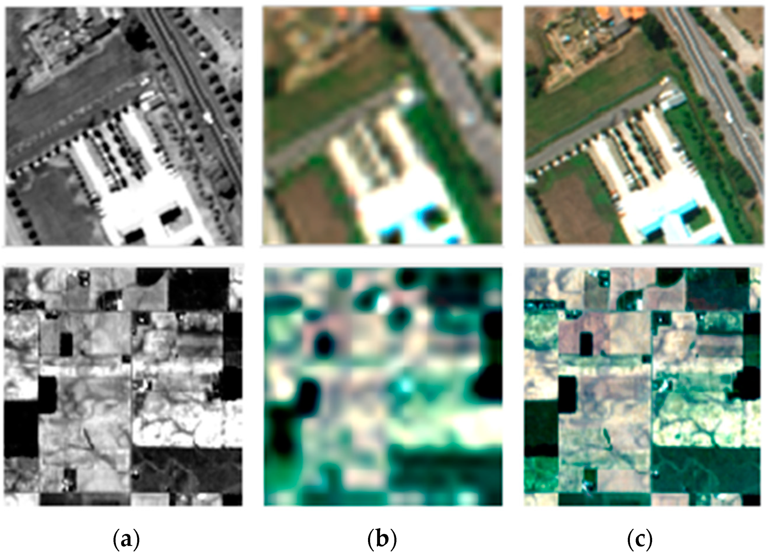
The proposed method CNTD is performed on two well-known data sets, depicted in Figure 3. The first data set is the Pavia University image [52], which is captured by the Reflective-Optics-System-Imaging-Spectrometer (ROSIS) optical sensor upon the Pavia University in Italy. The reference HRHSI is a image with 1.3 m per pixel spatial resolution. The wavelength domain from to mm is removed because of low SNR and water vapor absorptions. The LRHSI is produced by applying a Gaussian spatial blurring filter on each band of the reference image, and down-sampling with a factor of four in both width and height directions. The HRMSI of size is produced by filtering the reference image with the IKONOS-like reflectance spectral response function depicted in Figure 4. (see [19] for more details about SRF and PSF).
The Indian Pines image is the second test data set. It was acquired by the NASA Aeronautics-and-Space-Administration-Airborne-Visible-Infrared-Imaging-Spectrometer (AVIRIS) [53] over the Indian Pines scene situated in North-Western Indiana. The reference image of size has a wavelength domain from nm to nm and a m per pixel spatial resolution. We reduced its number of bands to 185 after removing the water absorption and noisy bands (–, –, –, and ). The LRHSI of size was constructed after down-sampling and application of the same blurring filters as which were applied to the first data set. The LANDSAT 7-like spectral response function, depicted in Figure 4, is engaged to produce a HRMSI of size . The reference, LRHSI and HRMSI of both data sets are depicted in Figure 3.
6.2. Evaluation Criteria
The performance of the proposed method is evaluated using five different indices. The first index, which is a measure of spectral distortion, is the spectral angle mapper (SAM) in degrees. The angle between pixel spectral responses and of the estimated HRHSI () and the reference image () are calculated, then averaged over all pixels. It is expressed as:
the ideal SAM value being zero.
The second index is the root mean squared error (RMSE) that evaluates the quality of the estimated HRHSI (), compared to the reference image (). It is defined as:
The third evaluation index is the relative dimensionless global error in synthesis (ERGAS), which measures the spectral quality of the estimated HRHSI, and is defined as:
where and denote the ith band of and , respectively. is the mean of . A lower ERGAS value means a lower spectral distortion between the estimated HRHSI () and the reference image (). In the case of perfect reconstruction, it is zero.
The degree of the distortion (DD) is the fourth index, defined as:
where is norm, and and are the vectorization of tensors and , respectively. The smaller the value of DD, the lower the spectral distortion.
The fifth index is the universal image quality index (UIQI) [54]. It is calculated by averaging over windows. The UIQI between the ith band of and is calculated by:
where d is the number of windows, and denote the jth window of the ith band of and , respectively, is the sample covariance between and , and are the mean and standard deviations of , respectively. The UIQI index between and is the average UIQI value of all bands, which is:
The ideal UIQI value is one.
All of the experiments were performed using MATLAB version R2016a, and have been run by a computer with an Intel Core i5 central processing unit (CPU) at 3.4 GHz and 32 GB random access memory (RAM).
6.3. Evaluation of the Parameters
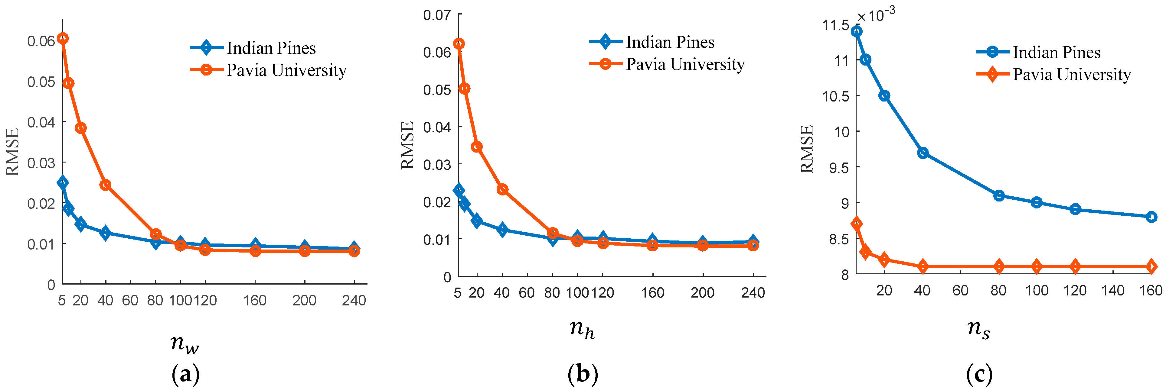
In order to evaluate the sensitivity of the proposed CNTD approach w. r. t. and its essential parameters, i.e., the number of mode (width, height, and depth) dictionary atoms , and , the proposed method has been performed for different numbers of mode-dictionary atoms. Figure 5a–c shows the RMSE of the estimated Pavia University and Indian Pines data sets as functions of the number of mode-dictionary atoms , and , respectively. As Figure 5a,b shows, the RMSE of both data sets strongly declines when and increase from 5 to 200. After that, the RMSE does not improve any further. Therefore, we chose to set the values of and to 167 for both data sets for all remaining experiments. As can be seen from Figure 5c, the RMSE for Pavia University decreases while increases from 5 to 40. For Indian Pines, the RMSE decreases as increases from 5 to 100, after which it does not decrease any further. Hence, we set to 30 for both aforementioned data sets. That the proposed CNTD method requires larger width and height mode-dictionaries compared to the spectral mode-dictionary is because generally the HSIs spectral vectors belong to a much lower dimension subspace.
6.4. Comparison with State of the Art Fusion Methods
The proposed fusion method is compared with state-of-the-art methods. In order to see the impact of non-negative priors, the CNTD method is compared with tensor decomposition methods CSFT [9] and NLSTF [23], which do not include non-negativity. Additionally, the proposed CNTD approach is compared with the well-known matrix framework CNMF [21], aiming to evaluate the ability of the proposed CNTD approach to preserve the spatio-spectral structure. Furthermore, our Tucker based method is compared with a CP tensor decomposition method, referred to as STEREO [43]. Finally, we have compared with the two-branched CNN method of [28].
The experiments validate the superiority of the proposed CNTD method on three aspects: the advantage of non-negative priors, the ability to preserve the spatio-spectral structure, and the computational complexity. RMSE, SAM, DD, ERGAS and UIQI for all approaches are shown in Table 2 and Table 3 for the Pavia University and Indian Pines data sets, respectively. To evaluate the computational complexity of the proposed method in comparison with the matrix-based method and the other tensor frameworks, the computation times of CNMF, CSTF, NLSTF and the proposed CNTD are shown in Table 4. The best values are depicted in bold.
It can be observed from Table 2 and Table 3 that the proposed method outperforms the other competing methods in terms of RMSE, DD, and UIQI indices, and shows promising results for the other indices. The proposed method outperforms CNMF, CNN and STEREO in almost all of the indices on both data sets. Of note, the efficiency of the CNN method highly depends on the training sample rate, while a huge amount of hyperspectral training data is practically unavailable. Furthermore, the proposed CNTD method outperforms the CSFT for most indices on both data sets. It also has better values of RMSE, DD, and UIQI than NLSTF.
As can be observed from Table 4, the proposed method is much more computationally efficient than the competing tensor-based approaches, and is comparable to the CNMF method. This agrees with the detailed description of the computational complexity in Section V. In contrast to the proposed method, for some of the state-of-the-art methods, such as CSTF and NLTF, the complexity increases faster than that which is linear with the size of the HSI cube.
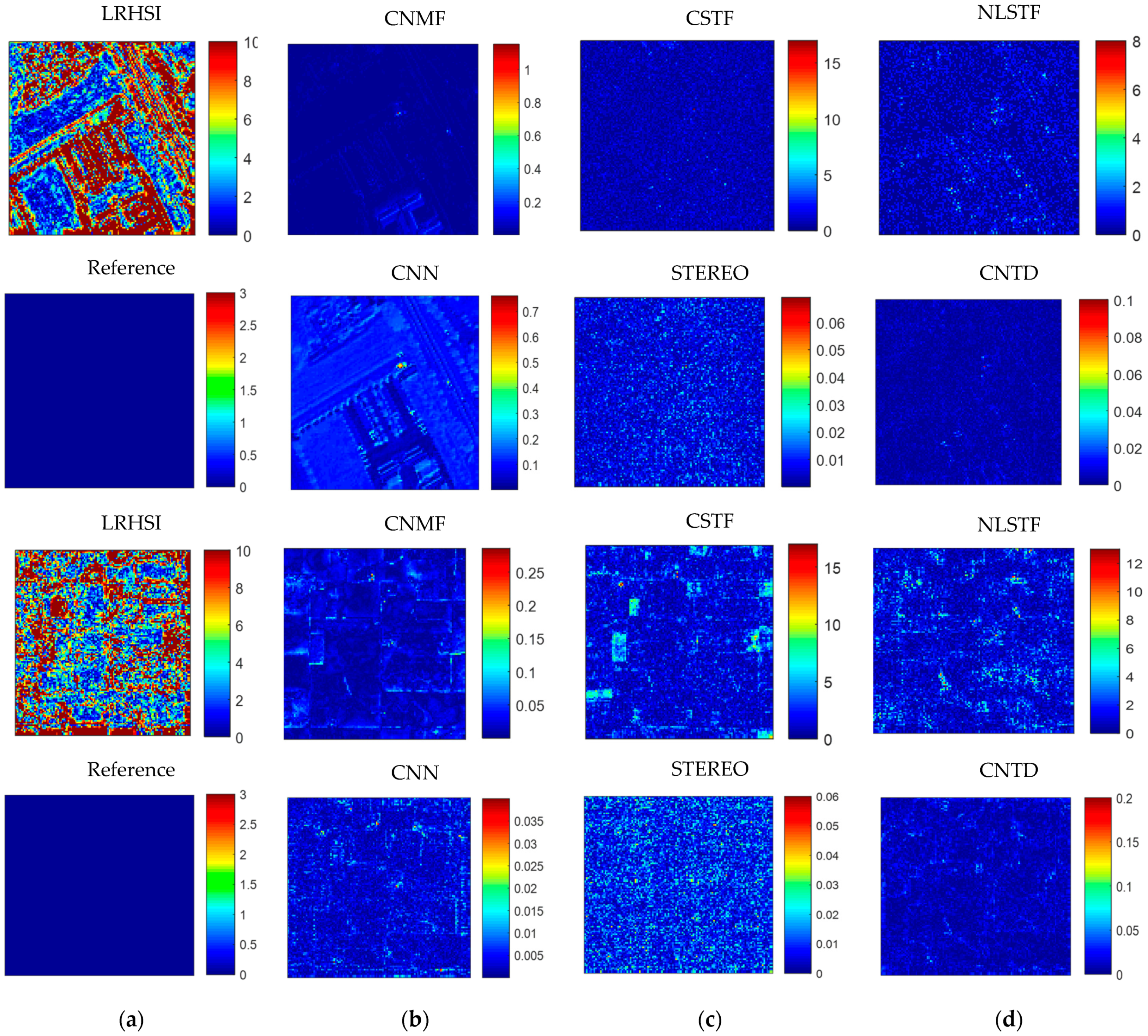
In order to validate the performance with respect to preserving spatial structures, in Figure 6, band 30 of the LRHSI and the estimated HRHSI with CNMF, CSTF, NLSTF, CNN, STEREO and the proposed CNTD are compared with the reference HRHSI. It can be observed that the proposed CNTD approach can correctly estimate most of the spatial details of the HRHSI, though there are a few distortions in the fusion results. Additionally, the error images of band 30, which reflect the differences between the estimated HRHSI and the reference image of both data sets are shown in Figure 7. The error images of the LRHSI, CNMF, CSTF, NLSTF, CNN, STEREO and the proposed CNTD are depicted. The proposed approach estimates spatial details of the HRHSI with much lower error than the competing methods. With CNMF and CNN, the edge structures of the HSI are lost, while CSTF, NLSTF and STEREO suffer from errors in homogeneous regions. The proposed approach performs better in preserving the spatial structures of HSIs at both edges and homogeneous regions.
7. Conclusions
The main objective of this paper was to extend the matrix formulation of non-negative matrix factorization to a tensor framework for the purpose of hyperspectral and multispectral image fusion. We proposed a coupled non-negative tensor decomposition approach that can be treated as a conventional NMF-based model. The proposed approach performs a tucker tensor factorization of a LRHSI and a HRMSI under the constraint of non-negative tensor decomposition. Unlike other state of the art methods, the complexity of the proposed approach is linear with the size of the HSI cube. The proposed approach gives competitive results with the state-of-the-art fusion approaches. As a future plan, we will incorporate prior information, such as spectral self-similarity, sparsity, smoothness and local consistence in the non-negative tensor decomposition, in order to find better unique basis vectors for the Tucker representation. Furthermore, in this paper we assumed the SRF and PSF to be known and also two input images considered to be registered. Therefore, we will try to overcome these limitations in our future work.
Author Contributions
M.Z.: conceptualization, methodology, software, writing, review and editing. M.S.H.: supervision. K.K. and P.S.: investigation, writing, review and editing. All authors have read and agreed to the published version of the manuscript.
Funding
This research received no external funding.
Acknowledgments
The authors would like to thank Jose Bioucas-Dias from the Instituto de Telecomunicaes and Instituto Superior Tecnico, Universidade de Lisboa for sharing the IKONOS-like reflectance spectral responses. Also, J. Inglada, from Centre National d’Études Spatiales, for providing the LANDSAT spectral responses used in the experiments. The authors also highly appreciate the time and consideration of the editors and the anonymous referees for their constructive suggestions that greatly improved the paper.
Conflicts of Interest
The authors declare no conflict of interest.
References
- Dian, R.; Fang, L.; Li, S. Hyperspectral image super-resolution via non-local sparse tensor factorization. In Proceedings of the IEEE Conference on Computer Vision and Pattern Recognition, San Juan, PR, USA, 17–19 June 1997; pp. 5344–5353. [Google Scholar]
- Kwan, C.; Choi, J.H.; Chan, S.H.; Zhou, J.; Budavari, B. A super-resolution and fusion approach to enhancing hyperspectral images. Remote Sens. 2018, 10, 1416. [Google Scholar] [CrossRef] [Green Version]
- Dian, R.; Li, S.; Fang, L.; Bioucas-Dias, J. Hyperspectral image super-resolution via local Low-rank and sparse representations. In Proceedings of the IGARSS 2018–2018 IEEE International Geoscience and Remote Sensing Symposium, Valencia, Spain, 22–27 July 2018; pp. 4003–4006. [Google Scholar]
- Dian, R.; Li, S.; Fang, L.; Wei, Q. Multispectral and hyperspectral image fusion with spatial-spectral sparse representation. Inf. Fusion 2019, 49, 262–270. [Google Scholar] [CrossRef]
- Dong, W.; Fu, F.; Shi, G.; Cao, X.; Wu, J.; Li, G.; Li, X. Hyperspectral image super-resolution via non-negative structured sparse representation. IEEE Trans. Image Process. 2016, 25, 2337–2352. [Google Scholar] [CrossRef]
- Ghasrodashti, E.; Karami, A.; Heylen, R.; Scheunders, P. Spatial resolution enhancement of hyperspectral images using spectral unmixing and bayesian sparse representation. Remote Sens. 2017, 9, 541. [Google Scholar] [CrossRef] [Green Version]
- Joshi, M.V.; Upla, K.P. Multi-Resolution Image Fusion in Remote Sensing; Cambridge University Press: Cambridge, UK, 2019. [Google Scholar]
- Lanaras, C.; Baltsavias, E.; Schindler, K. Hyperspectral super-resolution with spectral unmixing constraints. Remote Sens. 2017, 9, 1196. [Google Scholar] [CrossRef] [Green Version]
- Li, S.; Dian, R.; Fang, L.; Bioucas-Dias, J.M. Fusing hyperspectral and multispectral images via coupled sparse tensor factorization. IEEE Trans. Image Process. 2018, 27, 4118–4130. [Google Scholar] [CrossRef] [PubMed]
- Li, X.; Tian, L.; Zhao, X.; Chen, X. A super resolution approach for spectral unmixing of remote sensing images. Int. J. Remote Sens. 2011, 32, 6091–6107. [Google Scholar] [CrossRef]
- Wei, Q.; Bioucas-Dias, J.; Dobigeon, N.; Tourneret, J.-Y. Hyperspectral and multispectral image fusion based on a sparse representation. IEEE Trans. Geosci. Remote Sens. 2015, 53, 3658–3668. [Google Scholar] [CrossRef] [Green Version]
- Wei, Q.; Bioucas-Dias, J.; Dobigeon, N.; Tourneret, J.-Y.; Chen, M.; Godsill, S. Multiband image fusion based on spectral unmixing. IEEE Trans. Geosci. Remote Sens. 2016, 54, 7236–7249. [Google Scholar] [CrossRef] [Green Version]
- Yang, J.; Li, Y.; Chan, J.; Shen, Q. Image fusion for spatial enhancement of hyperspectral image via pixel group based non-local sparse representation. Remote Sens. 2017, 9, 53. [Google Scholar] [CrossRef] [Green Version]
- Akhtar, N.; Shafait, F.; Mian, A. Bayesian sparse representation for hyperspectral image super resolution. In Proceedings of the IEEE Conference on Computer Vision and Pattern Recognition, Boston, MA, USA, 7–12 June 2015; pp. 3631–3640. [Google Scholar]
- Zare, M.; Helfroush, M.S.; Kazemi, K. Fusing hyperspectral and multispectral images using smooth graph signal modelling. Int. J. Remote Sens. 2020, 41, 8610–8630. [Google Scholar] [CrossRef]
- Hardie, R.C.; Eismann, M.T.; Wilson, G.L. MAP estimation for hyperspectral image resolution enhancement using an auxiliary sensor. IEEE Trans. Image Process. 2004, 13, 1174–1184. [Google Scholar] [CrossRef]
- Nezhad, Z.H.; Karami, A.; Heylen, R.; Scheunders, P. Fusion of hyperspectral and multispectral images using spectral unmixing and sparse coding. IEEE J. Sel. Top. Appl. Earth Obs. Remote Sens. 2016, 9, 2377–2389. [Google Scholar] [CrossRef]
- Wei, Q.; Dobigeon, N.; Tourneret, J.-Y. Bayesian fusion of multi-band images. IEEE J. Sel. Top. Signal Process. 2015, 9, 1117–1127. [Google Scholar] [CrossRef] [Green Version]
- Simões, M.; Bioucas-Dias, J.; Almeida, L.B.; Chanussot, J. A convex formulation for hyperspectral image superresolution via subspace-based regularization. IEEE Trans. Geosci. Remote Sens. 2014, 53, 3373–3388. [Google Scholar] [CrossRef] [Green Version]
- Veganzones, M.A.; Simoes, M.; Licciardi, G.; Yokoya, N.; Bioucas-Dias, J.M.; Chanussot, J. Hyperspectral super-resolution of locally low rank images from complementary multisource data. IEEE Trans. Image Process. 2015, 25, 274–288. [Google Scholar] [CrossRef] [PubMed] [Green Version]
- Yokoya, N.; Yairi, T.; Iwasaki, A. Coupled nonnegative matrix factorization unmixing for hyperspectral and multispectral data fusion. IEEE Trans. Geosci. Remote Sens. 2012, 50, 528–537. [Google Scholar] [CrossRef]
- Dian, R.; Li, S.; Fang, L. Learning a low tensor-train rank representation for hyperspectral image super-resolution. IEEE Trans. Neural Netw. Learn. Syst. 2019, 30, 2672–2683. [Google Scholar] [CrossRef] [PubMed]
- Dian, R.; Li, S.; Fang, L.; Lu, T.; Bioucas-Dias, J.M. Nonlocal sparse tensor factorization for semiblind hyperspectral and multispectral image fusion. IEEE Trans. Cybern. 2019, 50, 4469–4480. [Google Scholar] [CrossRef] [PubMed]
- Xu, Y.; Wu, Z.; Chanussot, J.; Comon, P.; Wei, Z. Nonlocal coupled tensor cp decomposition for hyperspectral and multispectral image fusion. IEEE Trans. Geosci. Remote Sens. 2020, 58, 348–362. [Google Scholar] [CrossRef]
- Zhang, G.; Fu, X.; Huang, K.; Wang, J. Hyperspectral super-resolution: A coupled nonnegative block-term tensor decomposition approach. In Proceedings of the 2019 IEEE 8th International Workshop on Computational Advances in Multi-Sensor Adaptive Processing (CAMSAP), Guadeloupe, France, 15–18 December 2019; pp. 470–474. [Google Scholar]
- Sun, W.; Ren, K.; Meng, X.; Xiao, C.; Yang, G.; Peng, J. A band divide-and-conquer multispectral and hyperspectral image fusion method. IEEE Trans. Geosci. Remote Sens. 2021. [Google Scholar] [CrossRef]
- Yang, J.; Zhao, Y.-Q.; Chan, J.C.-W. Hyperspectral and multispectral image fusion via deep two-branches convolutional neural network. Remote Sens. 2018, 10, 800. [Google Scholar] [CrossRef] [Green Version]
- Zhang, L.; Nie, J.; Wei, W.; Li, Y.; Zhang, Y. Deep blind hyperspectral image super-resolution. IEEE Trans. Neural Netw. Learn. Syst. 2021. [Google Scholar] [CrossRef]
- Loncan, L.; De Almeida, L.B.; Bioucas-Dias, J.M.; Briottet, X.; Chanussot, J.; Dobigeon, N.; Fabre, S.; Liao, W.; Licciardi, G.A.; Simoes, M. Hyperspectral pansharpening: A review. IEEE Geosci. Remote Sens. Mag. 2015, 3, 27–46. [Google Scholar] [CrossRef] [Green Version]
- Lee, D.D.; Seung, H.S. Learning the parts of objects by non-negative matrix factorization. Nature 1999, 401, 788–791. [Google Scholar] [CrossRef] [PubMed]
- Jouni, M.; Dalla Mura, M.; Comon, P. Hyperspectral Image Classification Based on Mathematical Morphology and Using Tensor CP Decomposition. Math. Morphol.Theory Appl. 2019, 1, 1–30. [Google Scholar]
- Jouni, M.; Dalla Mura, M.; Comon, P. Classification of hyperspectral images as tensors using nonnegative CP decomposition. In Proceedings of the International Symposium on Mathematical Morphology and Its Applications to Signal and Image Processing, Saarbrücken, Germany, 8–10 July 2019; pp. 189–201. [Google Scholar]
- Zhao, G.; Tu, B.; Fei, H.; Li, N.; Yang, X. Spatial-spectral classification of hyperspectral image via group tensor decomposition. Neurocomputing 2018, 316, 68–77. [Google Scholar] [CrossRef]
- Das, S. Hyperspectral image, video compression using sparse tucker tensor decomposition. IET Image Process. 2021, 15, 964–973. [Google Scholar] [CrossRef]
- Fang, L.; He, N.; Lin, H. CP tensor-based compression of hyperspectral images. JOSA A 2017, 34, 252–258. [Google Scholar] [CrossRef]
- Huang, F.; Yu, Y.; Feng, T. Hyperspectral remote sensing image change detection based on tensor and deep learning. J. Vis. Commun. Image Represent. 2019, 58, 233–244. [Google Scholar] [CrossRef]
- Tan, J.; Zhang, J.; Zhang, Y. Target detection for polarized hyperspectral images based on tensor decomposition. IEEE Geosci. Remote Sens. Lett. 2017, 14, 674–678. [Google Scholar] [CrossRef]
- Li, S.; Wang, W.; Qi, H.; Ayhan, B.; Kwan, C.; Vance, S. Low-rank tensor decomposition based anomaly detection for hyperspectral imagery. In Proceedings of the 2015 IEEE International Conference on Image Processing (ICIP), Quebec City, QC, Canada, 27–30 September 2015; pp. 4525–4529. [Google Scholar]
- Fan, H.; Li, C.; Guo, Y.; Kuang, G.; Ma, J. Spatial–spectral total variation regularized low-rank tensor decomposition for hyperspectral image denoising. IEEE Trans. Geosci. Remote Sens. 2018, 56, 6196–6213. [Google Scholar] [CrossRef]
- Zhang, H.; Liu, L.; He, W.; Zhang, L. Hyperspectral image denoising with total variation regularization and nonlocal low-rank tensor decomposition. IEEE Trans. Geosci. Remote Sens. 2019, 58, 3071–3084. [Google Scholar] [CrossRef]
- Qian, Y.; Xiong, F.; Zeng, S.; Zhou, J.; Tang, Y.Y. Matrix-vector nonnegative tensor factorization for blind unmixing of hyperspectral imagery. IEEE Trans. Geosci. Remote Sens. 2017, 55, 1776–1792. [Google Scholar] [CrossRef] [Green Version]
- Kanatsoulis, C.I.; Fu, X.; Sidiropoulos, N.D.; Ma, W.-K. Hyperspectral super-resolution: Combining low rank tensor and matrix structure. In Proceedings of the 2018 25th IEEE International Conference on Image Processing (ICIP), Athens, Greece, 7–10 October 2018; pp. 3318–3322. [Google Scholar]
- Kanatsoulis, C.I.; Fu, X.; Sidiropoulos, N.D.; Ma, W.-K. Hyperspectral super-resolution: A coupled tensor factorization approach. IEEE Trans. Signal Process. 2018, 66, 6503–6517. [Google Scholar] [CrossRef] [Green Version]
- Cichocki, A.; Mandic, D.; De Lathauwer, L.; Zhou, G.; Zhao, Q.; Caiafa, C.; Phan, H.A. Tensor decompositions for signal processing applications: From two-way to multiway component analysis. IEEE Signal Process. Mag. 2015, 32, 145–163. [Google Scholar] [CrossRef] [Green Version]
- Cichocki, A.; Zdunek, R.; Phan, A.H.; Amari, S.-I. Nonnegative Matrix and Tensor Factorizations: Applications to Exploratory Multi-way Data Analysis and Blind Source Separation; John Wiley & Sons: Hoboken, NJ, USA, 2009. [Google Scholar]
- Zhou, G.; Cichocki, A. Fast and unique Tucker decompositions via multiway blind source separation. Bull. Pol. Acad. Sci. Tech. Sci. 2012, 60, 389–405. [Google Scholar] [CrossRef] [Green Version]
- Kim, Y.-D.; Choi, S. Nonnegative tucker decomposition. In Proceedings of the 2007 IEEE Conference on Computer Vision and Pattern Recognition, Minneapolis, MN, USA, 17–22 June 2007; pp. 1–8. [Google Scholar]
- Liu, X.; Xia, W.; Wang, B.; Zhang, L. An approach based on constrained nonnegative matrix factorization to unmix hyperspectral data. IEEE Trans. Geosci. Remote Sens. 2010, 49, 757–772. [Google Scholar] [CrossRef]
- Burred, J.J. Detailed derivation of multiplicative update rules for NMF. Paris Fr. 2014. Available online: https://www.semanticscholar.org/paper/Detailed-derivation-of-multiplicative-update-rules-Burred/3376b4df752f2428c451e530f9c6e0ce3a3f05e4 (accessed on 25 May 2021).
- Bioucas-Dias, J.M. A variable splitting augmented Lagrangian approach to linear spectral unmixing. In Proceedings of the 2009 First Workshop on Hyperspectral Image and Signal Processing: Evolution in Remote Sensing, Grenoble, France, 26–28 August 2009; pp. 1–4. [Google Scholar]
- Smith, L.N.; Elad, M. Improving dictionary learning: Multiple dictionary updates and coefficient reuse. IEEE Signal Process. Lett. 2012, 20, 79–82. [Google Scholar] [CrossRef]
- Dell’Acqua, F.; Gamba, P.; Ferrari, A.; Palmason, J.A.; Benediktsson, J.A.; Árnason, K. Exploiting spectral and spatial information in hyperspectral urban data with high resolution. IEEE Geosci. Remote Sens. Lett. 2004, 1, 322–326. [Google Scholar] [CrossRef]
- Green, R.O.; Eastwood, M.L.; Sarture, C.M.; Chrien, T.G.; Aronsson, M.; Chippendale, B.J.; Faust, J.A.; Pavri, B.E.; Chovit, C.J.; Solis, M. Imaging spectroscopy and the airborne visible/infrared imaging spectrometer (AVIRIS). Remote Sens. Environ. 1998, 65, 227–248. [Google Scholar] [CrossRef]
- Wang, Z.; Bovik, A.C. A universal image quality index. IEEE Signal Process. Lett. 2002, 9, 81–84. [Google Scholar] [CrossRef]
Figure 1.
Tensor factorization; (a) 3-dimensional tensor, (b) Tucker tensor decomposition.

Figure 2.
Illustration of the proposed CNTD method for hyperspectral and multispectral data fusion.

Figure 3.
Composite color images of (a) HRMSI, (b) LRHSI (c) reference images of the Pavia University data set (top row) and Indian Pines data set (bottom row).
Figure 3.
Composite color images of (a) HRMSI, (b) LRHSI (c) reference images of the Pavia University data set (top row) and Indian Pines data set (bottom row).

Figure 4.
Spectral response functions; (a) IKONOS like spectral response function, (b) LANDSAT 7-like spectral response function.
Figure 4.
Spectral response functions; (a) IKONOS like spectral response function, (b) LANDSAT 7-like spectral response function.

Figure 5.
The RMSE as function of the number of atoms , and for the proposed CNTD approach: (a) ; (b) ; (c) .
Figure 5.
The RMSE as function of the number of atoms , and for the proposed CNTD approach: (a) ; (b) ; (c) .

Figure 6.
Band 30 of the Pavia University (two top rows) and Indian Pines data sets (two bottom rows), respectively; the first and third rows (a) LRHSI, (b) CNMF, (c) CSTF, (d) NLSTF. The second and fourth rows (a) reference image, (b) CNN, (c) STEREO, (d) proposed CNTD.
Figure 6.
Band 30 of the Pavia University (two top rows) and Indian Pines data sets (two bottom rows), respectively; the first and third rows (a) LRHSI, (b) CNMF, (c) CSTF, (d) NLSTF. The second and fourth rows (a) reference image, (b) CNN, (c) STEREO, (d) proposed CNTD.

Figure 7.
The error images of the 30th band of Pavia University (two top rows) and Indian Pines data sets (two bottom rows), the first and third rows show the error image of (a) LRHSI, (b) CNMF, (c) CSTF, and (d) NLSTF. The second and fourth rows show the error images of (a) reference error image, (b) CNN, (c) STEREO, and (d) proposed CNTD method.


Table 1.
Basic Notation.
| Notation | Description |
|---|---|
| Tensor | |
| X | Matrix |
| Tensor element | |
| Spectral vector of tensor | |
| X | Scaler |
| Mode-n product | |
| Kronecker product | |
| Hadamard product | |
| Mode-n matricization of tensor X | |
| n mode matrix in Tucker decomposition |
Table 2.
Quantitative metrics of the different fusion methods on the Pavia University data set.
| Method | Pavia University Data Set | ||||
|---|---|---|---|---|---|
| RMSE | SAM | DD | ERGAS | UIQI | |
| Ideal value | 0.000 | 0.000 | 0.000 | 0.000 | 1.000 |
| CNMF [21] | 0.140 | 4.313 | 0.017 | 4.989 | 0.952 |
| CSTF [9] | 2.160 | 2.390 | 1.055 | 1.230 | 0.991 |
| NLSTF [23] | 1.452 | 0.964 | 0.846 | 0.520 | 0.993 |
| CNN [27] | 0.016 | 2.203 | 0.103 | 1.447 | 0.976 |
| STEREO [43] | 0.061 | 3.922 | 0.010 | 1.865 | 0.989 |
| CNTD method | 0.008 | 1.963 | 0.005 | 1.169 | 0.996 |
Table 3.
Quantitative metrics of the different fusion methods on the Indian Pines data set.
| Method | Indian Pines Data Set | ||||
|---|---|---|---|---|---|
| RMSE | SAM | DD | ERGAS | UIQI | |
| Ideal value | 0.000 | 0.000 | 0.000 | 0.000 | 1.000 |
| CNMF [21] | 0.054 | 2.142 | 0.008 | 1.789 | 0.954 |
| CSTF [9] | 1.533 | 1.363 | 0.997 | 1.082 | 0.974 |
| NLSTF [23] | 0.899 | 0.768 | 0.484 | 0.755 | 0.984 |
| CNN [27] | 0.013 | 2.270 | 2.090 | 1.060 | 0.820 |
| STEREO [43] | 0.042 | 2.303 | 0.007 | 2.538 | 0.932 |
| CNTD method | 0.009 | 1.661 | 0.006 | 1.249 | 0.972 |
Publisher’s Note: MDPI stays neutral with regard to jurisdictional claims in published maps and institutional affiliations. |
© 2021 by the authors. Licensee MDPI, Basel, Switzerland. This article is an open access article distributed under the terms and conditions of the Creative Commons Attribution (CC BY) license (https://creativecommons.org/licenses/by/4.0/).
Share and Cite
MDPI and ACS Style
Zare, M.; Helfroush, M.S.; Kazemi, K.; Scheunders, P. Hyperspectral and Multispectral Image Fusion Using Coupled Non-Negative Tucker Tensor Decomposition. Remote Sens. 2021, 13, 2930. https://0-doi-org.brum.beds.ac.uk/10.3390/rs13152930
AMA Style
Zare M, Helfroush MS, Kazemi K, Scheunders P. Hyperspectral and Multispectral Image Fusion Using Coupled Non-Negative Tucker Tensor Decomposition. Remote Sensing. 2021; 13(15):2930. https://0-doi-org.brum.beds.ac.uk/10.3390/rs13152930
Chicago/Turabian StyleZare, Marzieh, Mohammad Sadegh Helfroush, Kamran Kazemi, and Paul Scheunders. 2021. "Hyperspectral and Multispectral Image Fusion Using Coupled Non-Negative Tucker Tensor Decomposition" Remote Sensing 13, no. 15: 2930. https://0-doi-org.brum.beds.ac.uk/10.3390/rs13152930
Note that from the first issue of 2016, this journal uses article numbers instead of page numbers. See further details here.