Communication

Angle Estimation for MIMO Radar in the Presence of Gain-Phase Errors with One Instrumental Tx/Rx Sensor: A Theoretical and Numerical Study

1
College of Computer and Information Technology, Three Gorges University, Yichang 443000, China
2
College of Electronic Countermeasure, National University of Defense Technology, Hefei 230037, China
3
Nanjing Marine Radar Institute, Nanjing 211153, China
4
The 723th Research Institute of China State Shipbuilding Corporation, Yangzhou 225000, China
*
Author to whom correspondence should be addressed.
Remote Sens. 2021, 13(15), 2964; https://0-doi-org.brum.beds.ac.uk/10.3390/rs13152964
Submission received: 8 June 2021 / Revised: 23 July 2021 / Accepted: 26 July 2021 / Published: 28 July 2021
(This article belongs to the Special Issue Radar Signal Processing for Target Tracking)

Abstract

:
Ideal transmitting and receiving (Tx/Rx) array response is always desirable in multiple-input multiple-output (MIMO) radar. In practice, nevertheless, Tx/Rx arrays may be susceptible to unknown gain-phase errors (GPE) and yield seriously decreased positioning accuracy. This paper focuses on the direction-of-departure (DOD) and direction-of-arrival (DOA) problem in bistatic MIMO radar with unknown gain-phase errors (GPE). A novel parallel factor (PARAFAC) estimator is proposed. The factor matrices containing DOD and DOA are firstly obtained via PARAFAC decomposition. One DOD-DOA pair estimation is then accomplished from the spectrum searching. Thereafter, the remainder DOD and DOA are achieved by the least squares technique with the previous estimated angle pair. The proposed estimator is analyzed in detail. It only requires one instrumental Tx/Rx sensor, and it outperforms the state-of-the-art algorithms. Numerical simulations verify the theoretical advantages.

1. Introduction

Array radar is one of the most important techniques in remote sensing [1,2,3,4,5]. As a branch of active array radar, multiple-input multiple-output (MIMO) radar has gained extensive interest owing to the capability of waveform diversity (it emits mutual orthogonal waveforms using sensor array and receives the echoes using sensor array). To accurately estimate the direction-of-departure (DOD) and direction-of-arrival (DOA) is crucial to MIMO radar. In the past decades, many algorithms have emerged. Typical estimators include multiple signal classification (MUSIC) [6], Capon [7], estimation of signal parameters via rotational invariance techniques (ESPRIT) [8,9], parallel factor (PARAFAC) [10], etc. As reported in the literature, their excellent performances rely on ideal sensor response, i.e., transmitting and receiving (Tx/Rx) sensors are well-calibrated. In practice, unfortunately, unknown gain-phase errors (GPE) may exist in Tx/Rx arrays owing to hardware nonideality, which would bring perturbation to direction matrix, leading to a decline in estimation performance.
The GPE self-calibration issue has been extensively discussed in sensor arrays, but such a topic has always been overlooked in MIMO radar. Usually, the calibration issue in MIMO radar is much more complex than that in sensor array, because it often involves high-dimension array data processing. Several self-calibration methodologies have been proposed for MIMO radar with unknown GPE. In [11], a MUSIC-like framework was developed, which only needs one well-calibrated Tx/Rx sensor. The angles and GPE vectors are achieved via an alternative iteration method. Similar to the traditional counterparts, MUSIC-like is computationally unacceptable owing to exhaustive parameter search and slow convergence performance. Besides, it may occasionally fail since it usually gets stuck in the local minima. In [12], an ESPRIT-like method was introduced. The problem of DOD, DOA, and GPE vectors estimation is linked to a constrained optimization issue, and it is solved by Lagrange multiplier approach. It offers closed-form solutions to DOA and DOD estimation, so it is much more efficient than MUSIC-like. Another reduced-dimension MUSIC (RD-MUSIC) approach was derived in [13]. Therein, the estimation problem was transformed into a quadratic optimization issue, and DOD and DOA were separately obtained via two one-dimensional spatial spectrum searches. In [14], an improved ESPRIT method was presented, where rotational invariance property was only applicable to the data collected from the well-calibrated sensors. Therefore, the virtual aperture of MIMO radar was sacrificed. Recently, tensor algebra has brought new insight into this area. Benefiting from the tensor gain, the tensor methods usually provide more accurate decomposition results than the matrix approaches. By exploiting the tensor nature, the PARAFAC-like estimators were introduced in [15,16]. In both works, the factor matrices containing DOD and DOA were firstly achieved via PARAFAC decomposition. To estimate the angles and GPE vectors from the factor matrices, the Lagrange multiplier method was followed in [15], while the element-wise division operation was chosen in [16]. Another PARAFAC estimator was introduced in [17], which first estimates the gain error via element-wise division, and then it obtains the angle estimation via the least squares fitting. Finally, it achieves the phase errors with the estimated angles. More recently, an improved PARAFAC model was established in [18], which formulates the errors into an isolated factor matrix, and the iterative method is adopted to estimate the factor matrix. Unfortunately, the iteration is very sensitive to the initial values. Besides, the polarimetric signal model was investigated in [19], which calibrates the errors using an additional polarization resource. It should be pointed out that the methods in [12,13,14,16,17] require at least two auxiliary Tx/Rx sensors. Although the estimator in [15] works well with one well-calibrated Tx/Rx sensor, the array manifold must be strictly nonlinear, which limits its implementation.
To avoid the drawbacks pointed out previously, an improved PARAFAC-based estimator is proposed in this paper; the novelties of the proposed estimator are listed as follows:
  • Unlike the existing frameworks, the proposed estimator is suitable for MIMO radar with only one instrumental Tx/Rx sensor. This improvement benefits from the fact that the stochastic feature of the phase error is taken into account in the proposed estimator. Moreover, it is adaptive to arbitrary Tx/Rx sensor geometries;
  • The proposed estimator is computationally friendly. The DOD/DOA estimation in the proposed estimator can be accomplished via the combination of one-dimensional grid searching and least squares (LS) fitting. It does not involve eigen decomposition or high-dimension spectrum searching.
Owing to the above reasons, the proposed estimator is attractive from the perspectives of robustness, complexity, and accuracy. The identification ability as well as Cramer-Rao bound (CRB) of the proposed algorithm is analyzed. Numerical simulations are designed to verify the improvement of the proposed algorithm.

2. Problem Formulation

Throughout this paper, all the notations are the same to that in [8], unless otherwise specified.
We consider a bistatic MIMO radar configuration, which is equipped with M-element transmitting sensors and N-element receiving sensors. Both Tx/Rx arrays are uniform linear arrays (ULA) with the inter-element spacing d. We suppose the transmitting sensors simultaneously emit M orthogonal pulse waveforms. Assume there are K uncorrelated far field slow-moving targets appearing in the same range bin, let ϕ k and θ k be the DOD and DOA of the k-th ( k = 1 , 2 , , K ) target, respectively. The echoes of the targets are collected by the receiving array and passed through the matched filters. The noisy array measurement after matched filtering is given by [10].
x ( τ ) = k = 1 K [ a r ( θ k ) a t ( ϕ k ) ] b k ( τ ) + n ( τ )
where τ denotes the snapshot index, and b k ( τ ) denotes the complex envelope of the k-th target. n ( τ ) denotes the array noise, which is assumed to be Gaussian white. a t ( ϕ k ) M × 1 and a r ( θ k ) N × 1 are the k-th transmitting response vector (the phase shifts with respect to the reference sensor) and the receiving response vector, which are given by
{ a t ( ϕ k ) = [ 1 , exp ( j 2 π d sin ( ϕ k ) / λ ) , , exp ( j 2 π d ( M 1 ) sin ( ϕ k ) / λ ) ] T a r ( θ k ) = [ 1 , exp ( j 2 π d sin ( θ k ) / λ ) , , exp ( j 2 π d ( N 1 ) sin ( θ k ) / λ ) ] T
where λ is the wavelength of the carrier frequency. Specifically, suppose that GPE exists in both the Tx/Rx arrays. Then the model in (1) should be modified into [12,13,14,15,16,17]
x ( τ ) = k = 1 K [ ( C r a r ( θ k ) C t a t ( ϕ k ) ) ] b k ( τ ) + n ( τ )
where C t = G t P t M × M and C r = G r P r N × N are two diagonal matrices, whose diagonal elements denote the GPE of the transmitting array and receiving array, respectively. G t = diag { g t } , P t = diag { exp ( j p t ) } , G r = diag { g r } , P r = diag { exp ( j p r ) } , g t = [ g t 1 , g t 2 , , g t M ] T , p t = [ p t 1 , p t 2 , , p t M ] T , g r = [ g r 1 , g r 2 , , g r N ] T , p r = [ p r 1 , p r 2 , , p r N ] T , where g t m ( m = 1 , 2 , , M ) and g t n ( n = 1 , 2 , , N ) denote the gain errors associated with the m-th transmitting antenna and the n-th receiving antenna, and p t m and p r n denote the associated phase errors, respectively. Herein, the reference Tx/Rx sensor is assumed to be well-calibrated, e.g., g t 1 = g r 1 = 1 , p t 1 = p r 1 = 0 . Once L ( τ = 1 , 2 , , L ) snapshots are collected, (3) can be formulated in matrix format as
X = [ ( C r A r ) ( C t A t ) ] B T + N x = [ A ˜ r A ˜ t ] B T + N x
where A t = [ a t ( ϕ 1 ) , a t ( ϕ 2 ) , a t ( ϕ K ) ] M × K denotes the transmitting direction matrix; A r = [ a r ( θ 1 ) , a r ( θ 2 ) , a r ( θ K ) ] N × K denotes the receiving direction matrix; B = [ b 1 , b 2 , , b K ] L × K denotes the target reflection coefficient matrix; and b k = [ b k ( 1 ) , b k ( 2 ) , , b k ( L ) ] T , N x = [ n ( 1 ) , n ( 2 ) , , n ( L ) ] , A ˜ t = C t A t and A ˜ r = C r A r denote the associated perturbed direction matrices. Since the original direction matrices A t and A t are corrupted by the GPE matrices, thus the traditional subspace algorithms will fail to work.
It was pointed out that X can be formulated into a third-order tensor X N × M × L as [10]
X = k = 1 K a ˜ r , k a ˜ t , k b k + N
where N is the tensor format of the noise. According to [20] X can be interpreted as the Mode-3 unfolding of X Similarly, we can achieve another two matrices Y M L × N and Z N L × L , respectively, via Mode-1 and Mode-2 unfolding of X , which are given by
Y = [ A ˜ t B ] A ˜ r T + N y
and
Z = [ B A ˜ r ] A ˜ t T + N z
where N y and N z denote the rearranged array noise.

3. The Proposed Framework

The main steps of the proposed estimator are shown in Figure 1. It performs PARAFAC decomposition to acquire the corrupted direction matrices. Thereafter, it acquires the DOD/DOA via the combination of grid searching and the LS method. The details of the proposed approach will be shown next.

3.1. Estimation of the Corrupted Direction Matrices

Since the GPE matrices C t M × M and C r N × N are coupled with the direction matrices A t and A r , we need to achieve the corrupted response matrices A ˜ t and A ˜ r first. From the model in (5), they can be estimated via optimizing
min A ˜ t , A ˜ r , B X I × 1 A ˜ r × 2 A ˜ t × 3 B F
To tackle the above optimization issue, the trilinear alternating least squares (TALS) technique is commonly utilized. Since the tensor can be unfolded into matrices, the optimization in (8) is equivalently expressed as
{ min A ˜ t , A ˜ r , B X [ A ˜ r A ˜ t ] B T F min A ˜ t , A ˜ r , B Y [ A ˜ t B ] A ˜ r T F min A ˜˜ t , A ˜˜ r , B Z [ B A ˜ r ] A ˜ t T F
The main principle of TALS is to successively update one of A ˜ r , A ˜ t , and B via the LS technique and treat the remainder as known prior. For instance, if A ˜ r and A ˜ t are known, then B can be estimated via fitting the first item of (9), the LS solution of which is then given by
B ^ T = [ A ˜ r A ˜ t ] X
Similarly, once A ˜ t and B are estimated, we can further estimate A ˜ r via LS fitting the second item of (9), and the LS calculation of A ˜ r is
A ^ r T = [ A ˜ t B ] Y
In addition, with the previously estimated A ˜ r and B , we can estimate A ˜ t via the LS fitting of the last item in (9), from which one can obtain the LS update of A ˜ t as
A ^ t T = [ B A ˜ r ] Z
Usually, the LS updates in (10)–(12) will repeat before the convergence conditions, e.g., the fitting error is smaller than a fixed threshold. Although the TALS is guaranteed to converge, it suffers from the slow convergence speed. Herein, the well-known COMFAC algorithm in [21,22] is adopted to speed the iteration, which undergoes some pre-processing and can be quickly converged with only a few iterations.
Unlike the traditional matrix decomposition, PARAFAC decomposition is usually unique. For the model in (5), it was pointed out that if the Kruskal ranks of A ˜ r , A ˜ t and B (denoted by k r ( A ˜ r ) , k r ( A ˜ t ) and k r ( B ) , respectively) fulfill [10]
k r ( A ˜ r ) + k r ( A ˜ t ) + k r ( B ) 2 K + 2
then the estimations of A ˜ r , A ˜ t , and B are unique with permutations and scaling effect, i.e.,
{ A ^ t = A ˜ t Π Δ 1 + N 1 A ^ r = A ˜ r Π Δ 2 + N 2 B ^ = B Π Δ 3 + N 3
where Π is a permutation matrix, and Δ 1 , Δ 2 , and Δ 3 denote the corresponding scaler effects, which are diagonal scaling matrices and satisfy Δ 1 Δ 2 Δ 3 = I k . N 1 , N 2 , and N 3 are the fitting error matrices.

3.2. DOD and DOA Estimation

In what follows, we will show how to estimate the DOD from A ^ t , and the DOA can be estimated in a similar way from A ^ r . Before the detailed derivation, we assume that the phase errors are zero-mean random variables, i.e.,
{ E { ρ t } = 0 E { ρ r } = 0
The above hypothesis is always held for large scale arrays. It is easy to verify that
0 1 = 0 k Π
Besides, let a ^ t , k and a ˜ t , k stand for, respectively, the k-th column of A ˜ t and A ˜ t . Ignoring the noise item in a ^ t , k ,we can get a ^ t , k = δ a ^ t , k , where δ is a scalar. Define p m ( γ ) as
p m ( γ ) = { angle ( [ a ^ t , k ] m [ a t H ( γ ) ] m ) } 2
where [ a ] m denotes the m-th entity of a . Consequently, if γ = ϕ k , then p m ( γ ) = p t m 2 . Similar to [23], we construct the following spatial spectrum function
f ( γ ) = m = 2 M p m ( γ )
Notably, once γ = ϕ k , we have f ( γ ) = p t 2 2 + p t 3 2 + + p t M 2 . Replace sin ( γ ) with x, and then f ( γ ) can be rewritten as
g ( x ) = m = 2 M [ p t m + 2 π d m ( x sin ( ϕ k ) ) / λ ] 2
where d m = d ( m 1 ) . To find out the minimum value of g ( x ) , one can calculate the first derivative of g ( x ) and enforce it to zero, and then we can get the minimum point
x 0 = λ m = 2 M d m p t m 2 π m = 2 M d m 2 + sin ϕ k
In addition, let m ˜ denote the arithmetic mean of d m p t m , i.e.,
m ˜ = 1 M m = 2 M d m p t m
The mathematical expectation of m ˜ is
E { m ˜ } = 1 M m = 2 M E { d m p t m } = E { d p t }
It is easy to prove that m ˜ is an unbiased estimation. Then the mathematical expectation of x 0 is given by
E { x 0 } = λ M E { d p t } 2 π m = 2 M d m 2 + sin ϕ k
Since d and p t are independent, then we have E { d p t } = E { d } E { p t } . In combination with (15), it is easy to have
E { x 0 } = sin ϕ k
Therefore, by setting a series of search grids γ 1 , γ 2 , , γ Q , the first DOD can be estimated via finding the minimum value of f ( γ ) , e.g., ϕ ^ 1 = arg max γ f ( γ ) .
Although the rest DOD can be achieved in a similar method, it is computationally inefficient. Fortunately, the columns of A ˜ t suffer from the same GPE. Let h = angle ( a ˜ t , p . / a ˜ t , q ) , where . / represents the element-wise division [16]. Define
P t = [ 1   1     1 0   π ( M 1 ) π ] T
It is easy to find P t v = h , where v 2 × 1 is a vector with the second entity [ v ] 2 sin ( ϕ p ) sin ( ϕ q ) . Accordingly, let h ^ t , k = angle ( a ^ t , p . / a ^ t , q ) , and compute
v ^ t , k = P t h ^ t , k
After that, we can obtain the remainder (k = 2, 3…, K) DOD via
ϕ ^ k = arcsin ( [ v ^ ] 2 + sin ( ϕ ^ 1 ) )
Similarly, we can estimate all the DOA via one spatial spectrum search and K-1 LS fittings.

4. Algorithmic Analysis

4.1. Related Remarks

Remark 1.
From (14), one can observe that both A ^ t and A ^ t suffer from the same permutation Π Therefore, the estimated k-th DOD-DOA pair is paired automatically.
Remark 2.
Obviously, the proposed algorithm does not involve array geometry, but it can be easily extended to configuration with arbitrary array geometry, by adjusting the fitting matrix P t
.
Remark 3.
To simplify the derivation, we ignore the noise item in a ^ t , k , so the proposed algorithm works well at high signal-to-noise ratio (SNR), but may fail at low SNR.
Remark 4.
Once the DOD and DOA are obtained, the direction matrices A t and A r can be constructed. With the element-wise division technique in [16], one can easily achieve the estimated GPE matrices, and consequently the GPE self-calibration can be carried out by left multiplying X with C ^ r 1 C ^ t 1 , where C ^ r and C ^ t denote the estimations of C r and C t , respectively.
Remark 5.
The target reflection coefficient matrix B contains the Doppler information of target. Although the topic of estimate target Doppler frequency is interesting, it is beyond the scope of this paper.

4.2. Identifiability

The identifiability is equal to the maximum value K. (13) reveals the identifiability of the proposed estimator. Since we have max ( k r ( A ˜ t ) ) = M , max ( k r ( A ˜ r ) ) = N , when B is full Kruskal rank, (13) becomes
M + N + min ( L , K ) 2 ( K + 1 )
Generally, we have L ≥ K, so (28) is simplified as M + N K + 2 . It means that the proposed estimator can identify at most M + N 2 targets.

4.3. Deterministic CRB

The whole unknown parameter vector can be written as ξ = [ γ T , η T ] T , where γ = [ g t T , p t T , g r T , p r T ] T 2 ( M + N ) × 1 , η = [ θ t , 1 , θ t , K , ϕ t , 1 , θ r , k , ϕ r , K ] T 4 K × 1 . According to [12], the CRB on angle estimation is given by
CRB ( η ) = σ 2 2 [ J η η J γ η J γ γ 1 J γ η T ] 1
where Π A ˜ = I - A ˜ A ˜ , A ˜ = A ˜ r A ˜ t , J η η = τ = 1 L D τ H Π A ˜ D τ , J γ η = τ = 1 L D τ H Π A ˜ H τ , J γ γ = τ = 1 L H τ H Π A ˜ H τ with
D τ = [ a ˜ 1 b 1 ( τ ) θ t , 1 , , a ˜ b k ( τ ) ϕ t , k , a ˜ k b k ( τ ) θ r , k , , a ˜ K b K ( τ ) ϕ t , K ]
H τ = [ C g t 1 , , C p t m , , C g r n , , C p r n ] b l k d i a g { A b ( τ ) A b ( τ ) 2 ( M + N ) }
where b l k d i a g { · } denotes a block diagonal matrix.

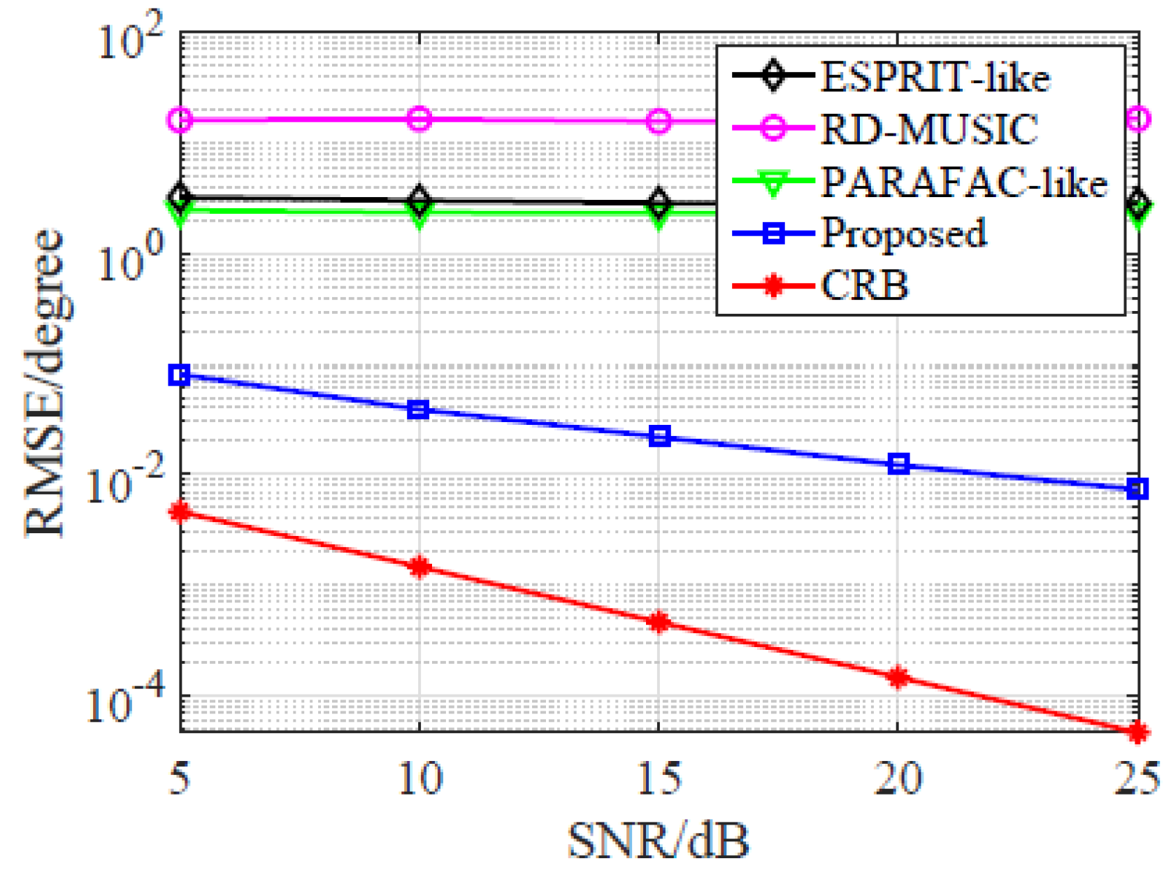
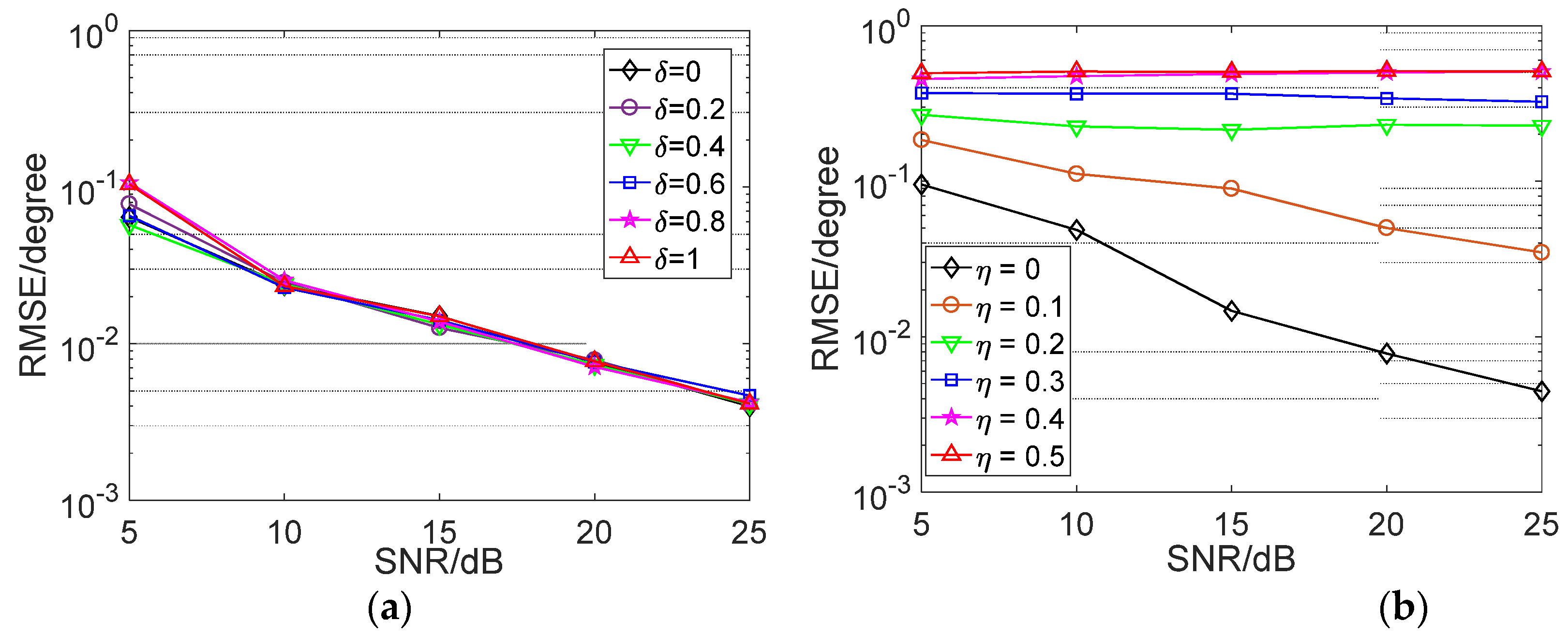
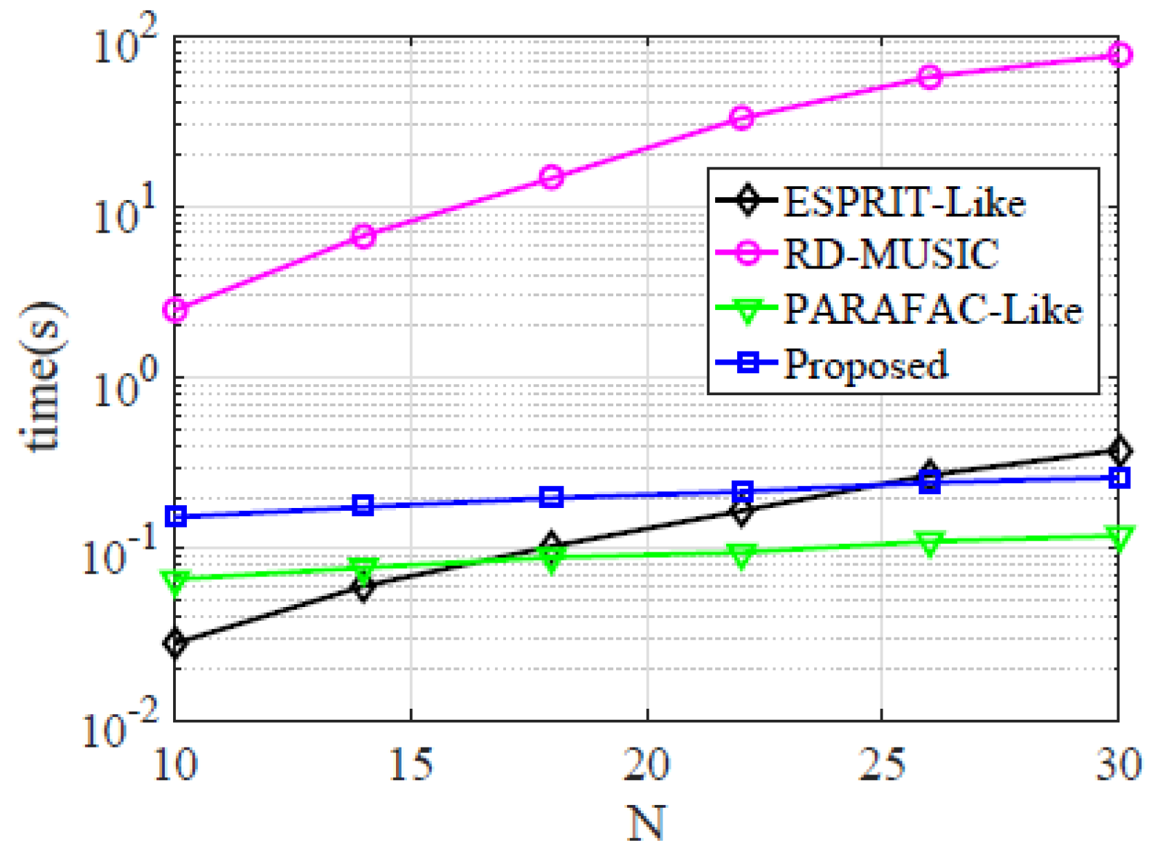
5. Simulation Results

Herein, Q = 200 Monte-Carlo simulation experiments are carried out to show the improvement of our estimator. Suppose that there are M = 11 transmitting sensors and N = 11 receiving sensors, both of which are half-wavelength spacing ULA. Consider that K = 3 targets are located at ( θ 1 , ϕ 1 ) = ( 10 , 15 ) , ( θ 2 , ϕ 2 ) = ( 20 , 25 ) and ( θ 3 , ϕ 3 ) = ( 30 , 35 ) , respectively. The following two cases are considered. Case (I): one instrumental Tx/Rx sensor with g t =[1, 1.26, 0.62, 1.09, 0.84, 0.56, 0.64, 1.03, 0.93, 1.06, 0.52]T and g r =[1, 0.6, 1.27, 1.34, 0.63, 1.42, 0.57, 1.15, 0.89, 0.75, 1.34]T; Case (II): three instrumental transmitting sensors and two instrumental receiving sensors with g t =[1, 1, 1, 1.07, 0.69, 1.17, 1.15, 1.43, 1.11, 1.3, 0.53]T and g r =[1, 1, 0.6, 1.27, 0.67, 1.17, 0.68, 1.15, 1.41, 0.72, 0.72, 1.31, 0.52, 0.78]T. In both cases, phase errors are randomly chosen from ±0.1, and L = 100. SNR in the simulation is defined as SNR = 10 lg ( X N x F 2 / N x F 2 ) [dB]. The root mean square error (RMSE) is utilized to assess the estimation accuracy, the definition of which is
R M S E = 1 Q q = 1 Q ( ϑ q ϑ 0 ) 2
where ϑ q is the estimated parameter in the q-th trial, and ϑ 0 is the true value. For comparison purpose, the performances of ESPRIT-like [12], RD-MUSIC [13], PARAFAC-like [15], and CRB are added (Matlab demo of the proposed algorithm can be found here).
Firstly, the average RMSE performances in Case I with various SNR are depicted in Figure 2. It is seen that the RMSE performances corresponding to ESPRIT-like, RD-MUSIC, and PARAFAC-like are at least an order of magnitude higher than the proposed estimator, and they barely vary with the increasing SNR. The observation indicates that ESPRIT-like, RD-MUSIC, and PARAFAC-like fail to work in such cases, since they need at least two well-calibrated Tx/Rx sensors. In contrast, average RMSE of the proposed estimator improves when SNR increases, which proves that the proposed estimator is suitable for the scenario with one instrumental Tx/Rx sensor.
Secondly, we plot the average RMSE of the proposed estimator vs. GPE ranges of our estimator in Case I. Herein, we consider the scenario that additional gain error δ is added to each sensor or additional phase error η is added to the mean of the phase errors. Figure 3 indicates the results. Obviously, the proposed estimator is insensitive to the gain error while it is sensitive to the mean of phase error. The mean of the phase errors in the proposed estimator must be strictly zero, otherwise it may fail to work.
Thirdly, we repeat the above simulation in Case II, and the result is shown in Figure 4. It is clearly observed that all the RMSE improve once SNR increases. Compared with ESPRIT-like, RD-MUSIC, and PARAFAC-like, the RMSE of the proposed estimator is about 10 dB lower. The observation may be caused by two reasons. On the one hand, the estimation accuracy of MUSIC is related to its search grid while ESPRIT-like suffers from the inaccurate GPE error matrices estimation. On the other hand, the eigen decomposition in both MUSIC and ESPRIT cannot exploit the tensor nature, leading to degraded subspace estimation. Notably, the proposed estimator always provides the lowest RMSE, which proves that the proposed estimator is superior to all comparison algorithms. However, it should be pointed out, as illustrated in Figure 2 and Figure 4, the distance between the proposed approach and CRB is big, so there is much room for further improvement.
Finally, the average run time of different algorithms versus N is given. In this experiment, M = 21, SNR = 15 dB, snapshot L = 500, gain errors, and phase errors are randomly chosen from [0.5,1.5] and ±0.1, respectively. It can be found in Figure 5 that the run time that RD-MUSIC required is at least 10 dB higher than the proposed estimator. Besides, the run time of our estimator is similar to that of PARAFAC-like (the gap is smaller than 5 dB), and the proposed estimator is more efficient than ESPRIT-like for large scale array.

6. Conclusions and Future Research

We have stressed the issue of joint angle and GPE self-calibration in bistatic MIMO radar system in this paper, where only one well-calibrated Tx/Rx sensor is considered. An improved PARAFAC estimator was proposed, the RMSE of which is an order of magnitude lower than that of the state-of-the-art PARAFAC-like method [15], while they offer comparable complexity. It should be a good choice for engineering application, especially in massive MIMO configuration. In the near future, more efforts should be devoted to verifying the proposed approach in the presence of real-life data.

Author Contributions

F.W.—designed the simulations and provided the draft; J.S. and X.W. and L.W.—helped to improve the writing. All authors have read and agreed to the published version of the manuscript.

Funding

This research was funded by National Natural Science Foundation of China under grant number 62071476.

Conflicts of Interest

The authors declare no conflict of interest.

References

  1. Liu, J.; Biondi, F.; Orlando, D.; Farina, A. Training data classification algorithms for radar applications. IEEE Signal Process. Lett. 2019, 26, 1446–1450. [Google Scholar] [CrossRef]
  2. Biondi, F.; Clemente, C.; Orlando, D. An atmospheric phase screen estimation strategy based on multichromatic analysis for differential interferometric synthetic aperture radar. IEEE Trans Geos. Remote Sens. 2019, 57, 7269–7280. [Google Scholar] [CrossRef]
  3. Biondi, F.; Addabbo, P.; Clemente, C.; Ullo, S.L.; Orlando, D. Monitoring of critical infrastructures by micromotion estimation: The mosul dam destabilization. IEEE J. Sel. Top. Appl. Earth Obs. Remote Sens. 2020, 13, 6337–6351. [Google Scholar] [CrossRef]
  4. Biondi, F.; Addabbo, P.; Clemente, C.; Orlando, D. Measurements of surface river doppler velocities with along-track InSAR using a single antenna. IEEE J. Sel. Top. Appl. Earth Obs. Remote Sens. 2020, 13, 987–997. [Google Scholar] [CrossRef]
  5. Biondi, F.; Clemente, C.; Orlando, D. An eigenvalue-based approach for structure classification in polarimetric SAR images. IEEE Geos. Remote Sens. Lett. 2020, 17, 1003–1007. [Google Scholar] [CrossRef] [Green Version]
  6. Yan, H.; Li, J.; Liao, G. multitarget identification and localization using bistatic MIMO radar systems. EURASIP J. Adv. Signal Process. 2008, 1, 48. [Google Scholar] [CrossRef] [Green Version]
  7. Bekkerman, I.; Tabrikian, J. Target detection and localization using MIMO radars and sonars. IEEE Trans. Signal Process. 2006, 54, 3873–3883. [Google Scholar] [CrossRef]
  8. Wen, F.; Shi, J.; Zhang, Z. Closed-form estimation algorithm for EMVS-MIMO radar with arbitrary sensor geometry. Signal Process. 2021, 186, 108117. [Google Scholar] [CrossRef]
  9. Wan, L.; Liu, K.; Liang, Y.C.; Zhu, T. DOA and polarization estimation for non-circular signals in 3-D millimeter wave polarized massive MIMO systems. IEEE Wirel. Commun. 2021, 20, 3152–3167. [Google Scholar] [CrossRef]
  10. Zhang, X.; Xu, Z.; Xu, L.; Xu, D. Trilinear decomposition-based transmit angle and receive angle estimation for multiple-input multiple-output radar. IET Radar Sonar Nav. 2011, 5, 626–631. [Google Scholar] [CrossRef]
  11. Liu, X.; Liao, G. Multitarget localization and estimation of gain phase error for bistatic MIMO radar. Acta Electron. Sin. 2011, 39, 596601. [Google Scholar]
  12. Guo, Y.; Zhang, Y.; Tong, N. ESPRIT-like angle estimation for bistatic MIMO radar with gain and phase uncertainties. Electron. Lett. 2011, 47, 996–997. [Google Scholar] [CrossRef]
  13. Li, J.; Zhang, X.; Cao, R.; Zhou, M. Reduced-dimension MUSIC for angle and array gain-phase error estimation in bistatic MIMO radar. IEEE Commun. Lett. 2013, 17, 443–446. [Google Scholar] [CrossRef]
  14. Li, J.; Jin, M.; Zheng, Y.; Liao, G.; Lv, L. Transmit and receive array gain-phase error estimation in bistatic MIMO radar. IEEE Antenn. Wirel. Propag. Lett. 2015, 14, 32–35. [Google Scholar] [CrossRef]
  15. Li, J.; Zhang, X.; Gao, X. A joint scheme for angle and array gain-phase error estimation in bistatic MIMO radar. IEEE Geos. Remote Sens. Lett. 2013, 10, 1478–1482. [Google Scholar] [CrossRef]
  16. Li, J.; Zhang, X. A method for joint angle and array gain-phase error estimation in bistatic multiple-input multiple-output non-linear arrays. IET Signal Process. 2014, 8, 131–137. [Google Scholar]
  17. Guo, Y.; Wang, X.; Wan, L.; Huang, M.; Shen, C.; Zhnag, K.; Yang, Y. Tensor-based angle and array gain-phase error estimation scheme in bistatic MIMO radar. IEEE Access 2019, 7, 47972–47981. [Google Scholar] [CrossRef]
  18. Sokal, B.; Gomes, P.R.B.; de Almeida, A.L.F.; Haardt, M. Tensor based receiver for joint channel, data, and phase-noise estimation in MIMO-OFDM systems. IEEE J. Sel. Top. Signal Process. 2021, 15, 803–815. [Google Scholar] [CrossRef]
  19. Kong, L.; Xu, X. Calibration of a polarimetric MIMO array with horn elements for near-field measurement. IEEE Trans. Antenn. Propag. 2020, 68, 4489–4501. [Google Scholar] [CrossRef]
  20. Kolda, T.G.; Bader, B.W. Tensor decompositions and applications. SIAM Rev. 2009, 51, 455–500. [Google Scholar] [CrossRef]
  21. Bro, R.; Sidiropoulos, N.; Giannakis, G. A fast least squares algorithm for separating trilinear mixtures. In Proceedings of the International Workshop on Independent Component Analysis and Blind Signal Separation, Aussois, France, 11–15 January 1999; pp. 289–294. [Google Scholar]
  22. Shi, J.; Wen, F.; Liu, T. Nested MIMO radar: Coarrays, tensor modeling and angle estimation. IEEE Trans Aero. Elec. Syst. 2021, 57, 573–585. [Google Scholar]
  23. Dai, Z.; Su, W.; Gu, H. A calibration method for linear arrays in the presence of gain-phase errors. IEICE Trans. Fund. Electr. 2020, 103, 2020. [Google Scholar] [CrossRef]
Figure 1. Illustration of the proposed estimator.
Remotesensing 13 02964 g001
Figure 2. Average RMSE vs. SNR in Case I.
Remotesensing 13 02964 g002
Figure 3. (a) Average RMSE vs. SNR with various gain error range δ, and (b) Average RMSE vs. SNR with various phase error range η.
Remotesensing 13 02964 g003
Figure 4. Average RMSE vs. SNR in Case II.
Remotesensing 13 02964 g004
Figure 5. CPU run time versus N in Case II.
Remotesensing 13 02964 g005
Publisher’s Note: MDPI stays neutral with regard to jurisdictional claims in published maps and institutional affiliations.

