A Photogrammetric-Photometric Stereo Method for High-Resolution Lunar Topographic Mapping Using Yutu-2 Rover Images

Abstract

Topographic products are important for mission operations and scientific research in lunar exploration. In a lunar rover mission, high-resolution digital elevation models are typically generated at waypoints by photogrammetry methods based on rover stereo images acquired by stereo cameras. In case stereo images are not available, the stereo-photogrammetric method will not be applicable. Alternatively, photometric stereo method can recover topographic information with pixel-level resolution from three or more images, which are acquired by one camera under the same viewing geometry with different illumination conditions. In this research, we extend the concept of photometric stereo to photogrammetric-photometric stereo by incorporating collinearity equations into imaging irradiance model. The proposed photogrammetric-photometric stereo algorithm for surface construction involves three steps. First, the terrain normal vector in object space is derived from collinearity equations, and image irradiance equation for close-range topographic mapping is determined. Second, based on image irradiance equations of multiple images, the height gradients in image space can be solved. Finally, the height map is reconstructed through global least-squares surface reconstruction with spectral regularization. Experiments were carried out using simulated lunar rover images and actual lunar rover images acquired by Yutu-2 rover of Chang’e-4 mission. The results indicate that the proposed method achieves high-resolution and high-precision surface reconstruction, and outperforms the traditional photometric stereo methods. The proposed method is valuable for ground-based lunar surface reconstruction and can be applicable to surface reconstruction of Earth and other planets.

1. Introduction

In lunar exploration, topographic mapping products, such as digital elevation model (DEM) and digital orthophoto map (DOM), are important for mission operations and scientific research. Orbital mapping provides large-area products for topographic analysis, geological characterization and other scientific investigations [1,2,3], and ground-based mapping using rover stereo imagery has been routinely applied in landing missions to support surface operations and in-situ scientific explorations [4,5,6,7,8]. Image matching is of particular importance in topographic mapping using rover stereo images [9]. However, sometimes the application of image matching is limited due to stereo imaging quality and insufficient image texture. Moreover, stereo images could not be acquired due to payload limit under some circumstances. For example, Chang’e-4 lander carried a terrain camera, which is located on top of the lander [10]. It can rotate 360° horizontally to obtain a panoramic view of the lunar surface, but without stereo imaging capability. In these cases, ground-based high-precision topographic mapping becomes very challenging.

In the field of computer vision, shape from shading (SfS) technique has long been studied to estimate the shape of an object from one image on the basis of the surface photometry, the position of light, and the viewing directions [11,12]. As an extension to the original single image SfS, the photometric stereo method can recover albedo and local surface shape at pixel-level with more than two images of the same scene taken under different illumination conditions [13]. Photometric stereo techniques have been developed for lunar and planetary surface reconstruction [14,15,16,17,18] to improve the quality of mapping products and generate pixel-level DEMs where image matching fails [14,19]. It is noted that these lunar and planetary researches all use orbital images to generate mapping products, and both the viewing angle and illumination angle of the images are different.

Following the work of Woodham [13], the traditional photometric stereo method assumes orthographic projection and Lambert reflectance model. This simple reflectance model can be reasonable for certain types of materials, and orthographic projection is appropriate when objects are far away from the camera, e.g., in the case of orbital images. Since the rover imaging are significantly off-nadir, they cannot be simplified as orthographic projection, perspective projection with collinearity equations should be more accurate. Meanwhile, various lunar reflectance models can be used for lunar rover mapping. Thus, it would be valuable to integrate photometric stereo with collinearity equations and lunar reflectance model for rover image-based surface reconstruction when stereo-photogrammetric method is not applicable.

This paper proposes a novel photogrammetric-photometric stereo (PPS) method based on the collinearity equation and reflectance model for ground-based mapping of the lunar surface. The PPS method is able to generate a height map from multiple rover images acquired under different illumination conditions and the same viewing condition. The paper is organized as follows: Section 2 summarizes related studies, and Section 3 describes the proposed PPS method in detail. The experimental results using simulated images and lunar surface images captured by Yutu-2 navigation camera (Navcam) are presented in Section 4. Section 5 provides a brief discussion and the concluding remarks.

2. Related Work

Topographic reconstruction of the lunar surface is critical to engineering applications and scientific research. Traditional 3D reconstruction techniques based on photogrammetry have been widely applied in lunar topographical mapping using stereo orbital images [20] or stereo rover images [4,5]. Some software packages have been developed for planetary image mapping, such as ASP [21], SOCET SET [22], dense matcher [23], and Planetary3D [24].

In general, the key techniques of orbital image mapping include construction of geometric model, bundle adjustment, dense image matching, and point cloud generation. So far, most studies use a rigorous physical sensor model based on collinearity equations, e.g., geometric parameters of a terrain camera (TC), lunar reconnaissance orbiter camera (LROC), narrow angle camera (NAC) images, Chang’e-1 (CE-1), Chang’e-2 (CE-2) images are refined to improve mapping accuracy based on a rigorous sensor model [25,26,27,28,29]. Recently, the rational function model (RFM) for geometric modelling has been developed [30,31,32,33]. After block adjustment based on RFM, the residual is less than 1 pixel, precise topographic models are generated from CE-1, CE-2, and NAC images [31,33,34]. Image matching is a crucial step in orbital photogrammetric processing. The scale invariant feature transform (SIFT) algorithm has been used for feature matching [35]. Based on matched feature points, epipolar constraints and spatial constraints are used to generate dense points. Delaunay triangulation is used to predict the approximate corresponding locations of other non-feature points [36,37]. Dense matching algorithm, such as semi-global matching (SGM), has been adopted in orbital mapping [38,39]. Recently, to deal with matching images with illumination differences, a photoclinometry assisted image matching (PAM) approach is developed in the image matching to create pixel-wise matches [40].

Compared with the orbital data, ground images obtained by rover cameras can provide high accuracy in situ measurements at centimeter resolution. Stereo rover images have been routinely used to generate DEMs and DOMs for mission operations and scientific investigations in Chang’e-3 and Chang’e-4 rover missions [4,5].

The early algorithms of SfS were initiated since 1970s [11,12], and laid the foundation of photoclinometric surface reconstruction. Based on the image irradiance equation, with corresponding reflectance model, these algorithms estimate the surface slopes and heights of each pixel. Many SfS methods are built upon specific geometry conditions and limited properties of reflectance [13,16,17]. Although such methods can reconstruct reasonable 3D models, they are restricted to benchmark datasets and indoor images. Planetary images (e.g., Moon and Mars images) generally have subtle albedo variations and trivial reflectance diversities [41], these characteristics make them suitable for reconstructing DEM using SfS techniques. Actually, SfS has been further developed and applied in planetary mapping and relevant scientific research [42,43,44]. For instance, the SfS derived DEMs (together with stereo derived DEMs) were used for safety assessment of the Mars exploration rovers (MER) landing sites [45], the candidate Mars science laboratory (MSL) landing sites evaluation [46], and topographic analysis of Chang’e-4 landing site [47]. Moreover, SfS derived DEMs have also been used in spectral analysis of the lunar surface [48], lunar soil strength estimation based on Chang’e-3 images [49], concreted fragments analysis at Chang’e-4 landing site [50], and fine-scale analysis of craters and rocks at the Chang’e-4 landing site [40]. Photoclinometric surface reconstruction performs well in local scale reconstruction but has poor large scale accuracy. Hence, in recent years, methods have been developed to incorporate existing low-resolution 3D information (e.g., low-resolution DEMs from photogrammetry or laser altimetry) into photoclinometry [16,17,51,52] and improved results have been achieved.

To overcome the uncertainty from the single-image SfS, photometric stereo method has been developed to estimate the local surface orientation by using several images of the same surface taken from the same viewpoint but under illuminations from different directions [13]. The method first recovers surface gradients from the overdetermined equations, and then integrates the gradient field to determine the 3D surface. As multiple images with different illuminations yield redundancy, the photometric stereo method can improve the accuracy of surface reconstruction. It has been applied to close-range and small-scale scene reconstruction [53]. In the field of planetary mapping, the multi-image shape from shading (MI-SfS) algorithm was developed [14]. The core concept of MI-SfS is similar to photometric stereo and it was able to produce high resolution lunar DEMs when image matching fails due to lack of distinctive texture. This method was further investigated in lunar mapping [19,54], and pixel-level resolution mapping results at Chang’e-4 and Chang’e-5 landing sites are achieved [19].

In regard to photoclinometric surface reconstruction for rover images, several methods have been proposed to derive detailed topography. For Chang’e-3 rover images, a linear approximation photoclinometry algorithm is applied to generate a DTM in 3-dimensional pixel scale, and the relationship between disparity and height is used to calculate the soil strength [49]. Wu et al. [40] presented an approach by integrating photogrammetry and photoclinometry for centimeter-resolution modelling from Yutu-2 stereo Pancam images. Firstly, photogrammetry processing of stereo images is completed to generate a DEM and an orthoimage mosaic of the landing site [40]. Then the DEM is refined to higher resolution using photoclinometry. The same procedure is also applied to derive the detailed topography for target crater analysis [50]. In summary, this rover-based method mainly include stereo photogrammetry processing and photoclinometry refinements, stereo photogrammetry provides an initial DEM and phototoclinometry retrieves fine-grained details and complement the limitations of dense image matching. However, while the rover-based methods depend on the photogrammetry processing of stereo images, PPS approach integrates photometric stereo with collinearity equations, it can reconstruct topography directly from multiple monocular images. As multiple images with different illuminations provide redundancy, PPS can provide reliable reconstruction results. Furthermore, as the images are obtained by the rover cameras at the same location, it is not necessary for images co-registration.

It is well noted that the traditional photometric stereo algorithm assumes orthographic projection and Lambertian surface. The method has been extended from different aspects to deal with general materials, unknown lighting and reflection [55,56], and perspective camera model [57]. Particularly, Tankus and Kiryati [57] introduced the image irradiance equations under the perspective projection model with identity rotation matrix, and developed the solution to a set of three image irradiance equations, which provided better accuracy than that under orthographic projection. The orthographic projection used in traditional photometric stereo is not appropriate for rover images. Firstly, the distance between rover camera and the lunar surface is close, secondly a pitch angle is usually set for the rover camera, the rotation matrix is not the identity matrix. Thus, the traditional photometric stereo method should be improved to accommodate rover images. The proposed PPS method integrates photogrammetry collinearity equations and lunar reflectance model, which extends the photometric stereo method for ground-based lunar topographic mapping.

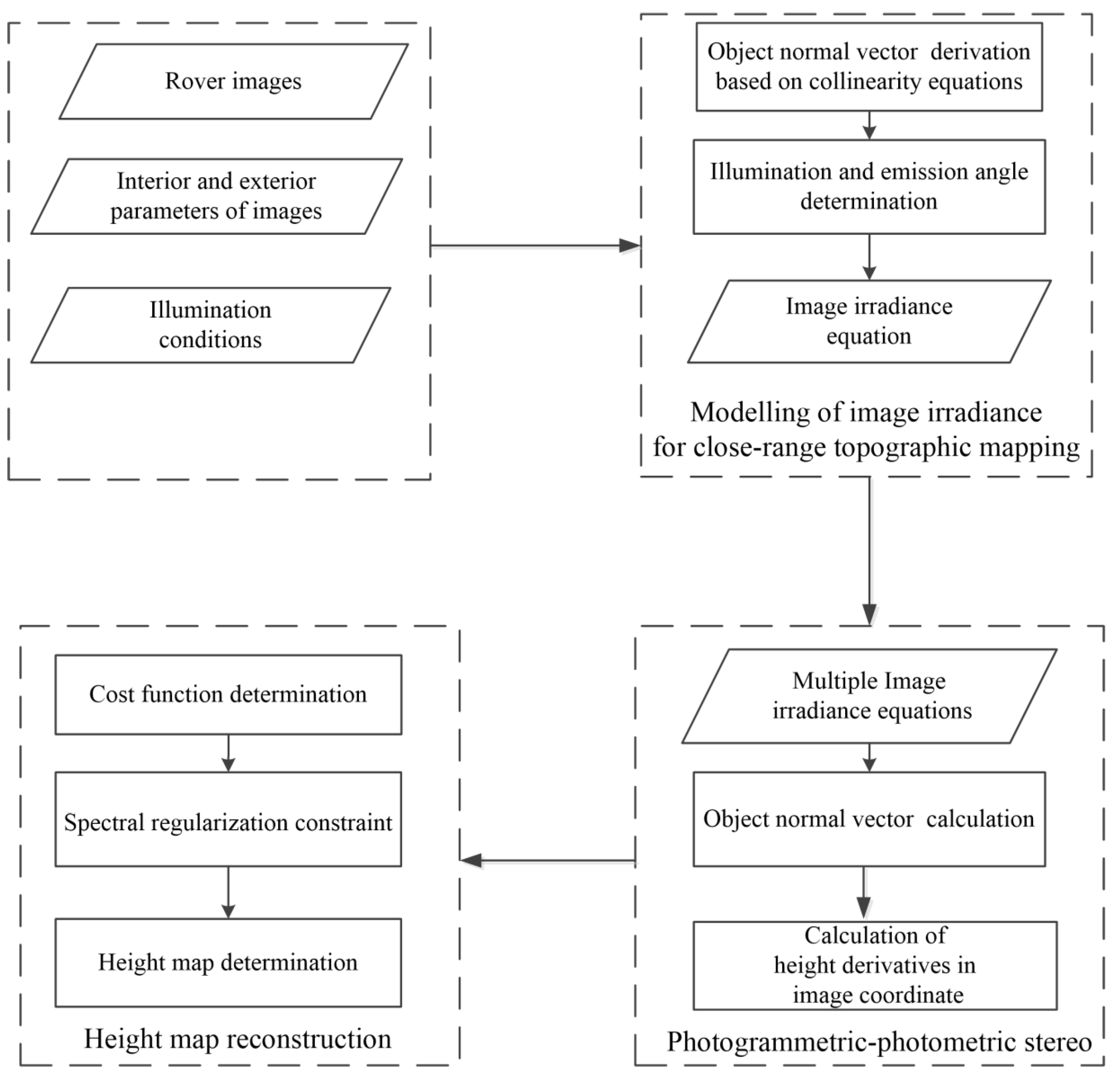
3. Photogrammetric-Photometric Stereo Method

The framework of the PPS for lunar rover images is illustrated in Figure 1. First, the imaging irradiance equation of close-range topographic mapping is introduced based on collinearity equations and lunar reflectance model, and the relationship between surface height value and image gray value can be obtained. It can be applied in general cases of photogrammetry, when the rotation matrix is not the identity matrix. Second, the solution of photometric stereo for close-range topographic mapping is derived based on multiple perspective image irradiance equations, and height derivatives can be estimated by iterative calculation. Finally, the global least-squares surface reconstruction with spectral regularization is used to attain the height value from the estimated gradient.

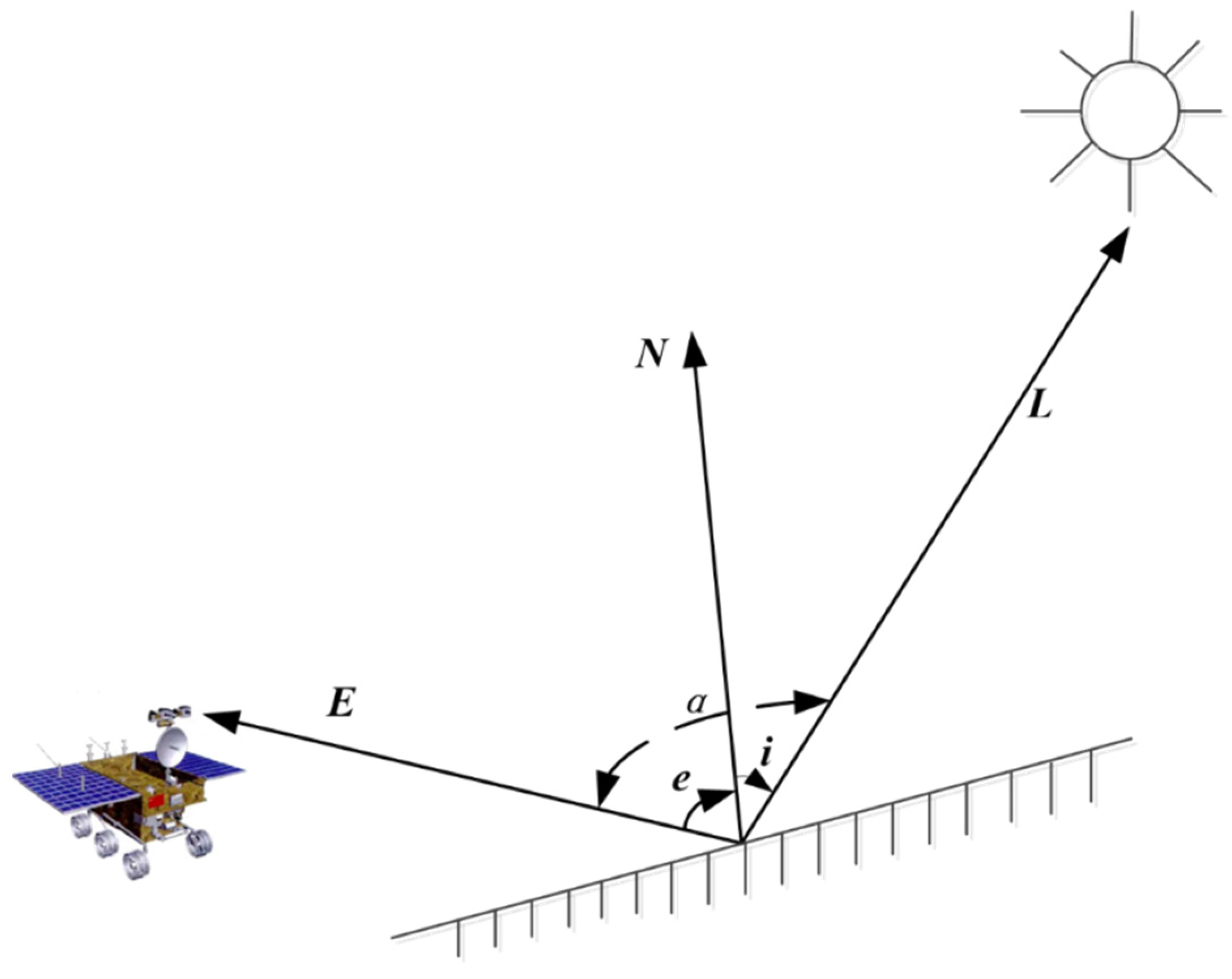
3.1. Modelling the Image Irradiance for Close-Range Topographic Mapping

The modelling of the image formation process defines the process between the surface shape and the projected image intensity, which is crucial for photometric stereo problem. The image intensity of a pixel depends mainly on the projection model, the surface reflectance property, surface orientations, and the direction of the illumination. Figure 2 shows relationships of the rover image formation, where L is the incident illumination direction vector, N is the normal vector of the surface, and E is the viewing direction, and the incidence angle i is formed between the vector of solar ray and the normal vector of the surface, the emission angle e is formed between the vector pointing to the sensor and the normal vector of the surface, and $\alpha$ is the phase angle between the solar ray and camera.

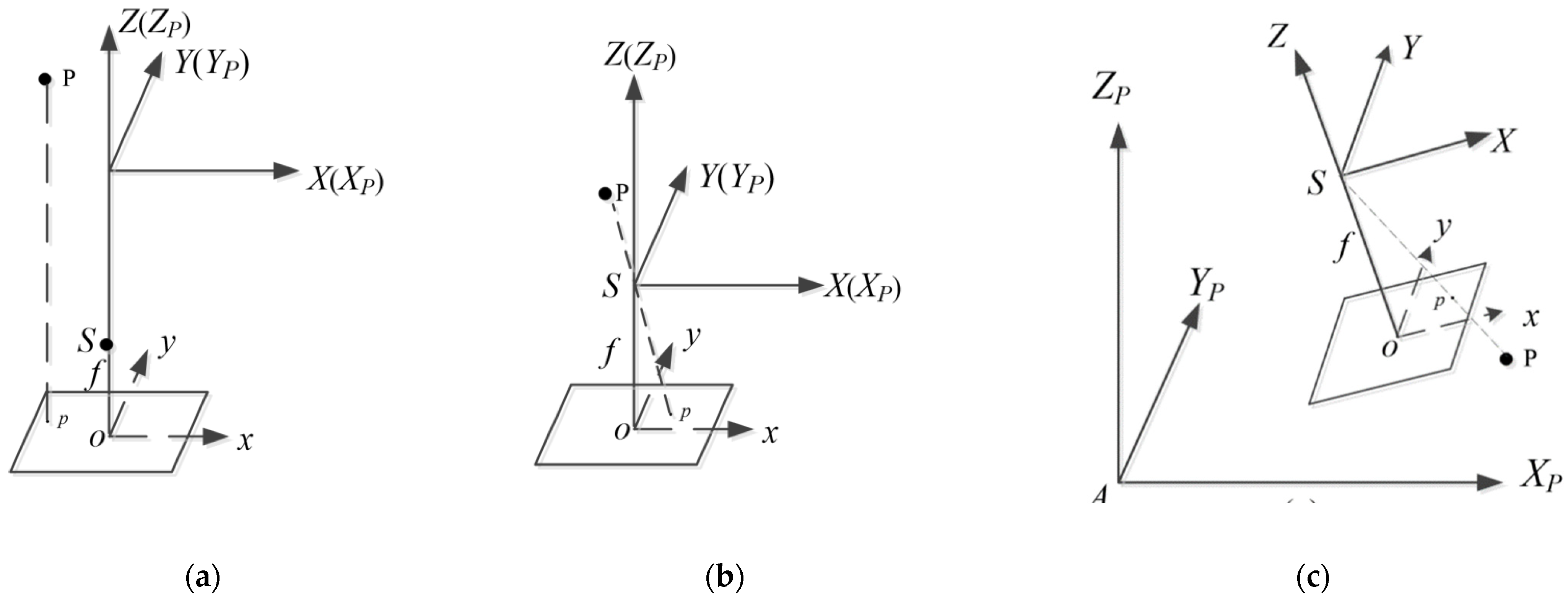
3.1.1. Coordinates in Traditional Photometric Stereo vs. Coordinates in PPS

As Figure 3a shows, for most photometric stereo applications [55,56], the origin of the object coordinate system is at the optical center S of the camera, f is the focal length, the axes of X, and Y are parallel to the x and y axes of the image plane, respectively. Furthermore, orthographic projection is assumed, so that the camera is considered to be far from the surface relative to the size of the scene. The light source is regarded as a point source at infinite distance and therefore constant illumination is assumed over the entire scene.

Assuming height Z is differentiable with respect to X and Y, the normalized surface normal $\widehat{N}$ can be represented in terms of partial derivatives of Z with respect to X and Y [58].

$$\widehat{N}=\frac{\left(-\frac{\partial Z}{\partial X},-\frac{\partial Z}{\partial Y},1\right)}{\sqrt{{(\frac{\partial Z}{\partial X})}^2+{(\frac{\partial Z}{\partial Y})}^2+1}},$$

(1)

where $\left(\frac{\partial Z}{\partial X},\frac{\partial Z}{\partial Y}\right)$ represents the partial derivatives of Z in X and Y directions.

The orthographic projection is widely used in traditional photometric stereo for orbital mapping. The partial derivatives of height Z w.r.t. x and y, which are described as $\frac{\partial Z}{\partial x}$ and $\frac{\partial Z}{\partial y}$, are always used to represent the surface normal, and as the resolution is the same for each pixel, there is

$$\begin{gathered} \frac{\partial Z}{\partial X}=m\frac{\partial Z}{\partial x}=m{Z}_x \\ \frac{\partial Z}{\partial Y}=m\frac{\partial Z}{\partial y}=m{Z}_y \end{gathered}$$

(2)

The scaling factor m is usually set to 1 for convenience.

Figure 3b shows the image and object coordinates under perspective projection. The image coordinate is o-xy, the object coordinate is S-XYZ. The surface normal is derived as in [59]

$$\stackrel{\wedge }{N}=\frac{\left(f{Z}_x,f{Z}_y,x{Z}_x+y{Z}_y+Z\right)}{\sqrt{{(x{Z}_x+y{Z}_y+Z)}^2+f^2\left(Z_x^2+Z_y^2\right)}}$$

(3)

where (x,y) is the perspective projection of (X, Y, Z) with identity matrix as the rotation matrix, that is

$$\begin{gathered} X=-\frac{xZ}{f}, \\ \mathrm{Y}=-\frac{yZ}{f}, \end{gathered}$$

(4)

However, to facilitate topographic mapping, rover localization, and path planning, rotation angles of rover cameras are used [5]. The rotation angles are not small angles, and, thus, cannot be approximated as zero. Figure 3c shows the image and object coordinates for PPS. The image coordinate is o-xy, the object coordinate is A-X_PY_PZ_P, and it is well noted that the axes of X_P, Y_P in object space are not parallel to x, y axes of the image plane. For rover orthorectified images, the axes of X_P, Y_P in object space are parallel to x, y axes of the image plane, traditional photometric stereo can be used. However, new image irradiance equations should be developed for original rover images with perspective projection. In summary, the following aspects should be considered when developing a proper image irradiance equation for rover-based lunar surface mapping: (1) The pitch angle of the camera cannot be ignored, and the rotation matrix cannot be treated as identity matrix; (2) Objects are not often located very far from the camera as the camera is close to the ground; (3) The axes of X_P, Y_P are not parallel to x, y of the image plane. Thus the surface normal should be deduced based on the principles of photogrammetry and photometric stereo.

3.1.2. Modelling of Surface Normal Based on Collinearity Equations

To make the photometric stereo algorithm useful, a general imaging irradiance equation is introduced based on photogrammetric collinearity equations, illumination conditions and camera interior and exterior orientation parameters.

As the object coordinates X, Y are unknowns, the surface normal can be derived from the collinearity equations.

$$\begin{gathered} x-x_0=-f\frac{a_1\left(X-X_s\right)+b_1\left(Y-Y_s\right)+c_1\left(Z-Z_s\right)}{a_3\left(X-X_s\right)+b_3\left(Y-Y_s\right)+c_3\left(Z-Z_s\right)} \\ {y}_0-y=-f\frac{a_2\left(X-X_s\right)+b_2\left(Y-Y_s\right)+c_2\left(Z-Z_s\right)}{a_3\left(X-X_s\right)+b_3\left(Y-Y_s\right)+c_3\left(Z-Z_s\right)}, \end{gathered}$$

(5)

In the equations, (x,y) represents the coordinate of the image point in the image plane coordinate system; (X, Y, Z) is the object coordinate in the object coordinate system; (X_S, Y_S, Z_S) represents three translation components of the exterior orientation parameters of the camera; (a₁, a₂, a₃,…, c₃) stands for the elements of the rotation matrix; (x₀, y₀) is the principle point position, f represents the principal distance of the camera.

In order to simplify the derivation process, the following symbols are used

$$\begin{gathered} \tilde{X}=X-X_S \\ \tilde{Y}=Y-X_S \\ \tilde{Z}=Z-Z_S, \\ \tilde{x}=x-x_0 \\ \tilde{y}=y_0-y \end{gathered}$$

(6)

The derivatives can be calculated as

$$\begin{gathered} \frac{\partial \tilde{Z}}{\partial \tilde{X}}=\frac{\partial \tilde{Z}}{\partial x}·\frac{\partial x}{\partial \tilde{X}}+\frac{\partial \tilde{Z}}{\partial y}·\frac{\partial y}{\partial \tilde{X}} \\ \frac{\partial \tilde{Z}}{\partial \tilde{Y}}=\frac{\partial \tilde{Z}}{\partial x}·\frac{\partial x}{\partial \tilde{Y}}+\frac{\partial \tilde{Z}}{\partial y}·\frac{\partial y}{\partial \tilde{Y}}, \end{gathered}$$

(7)

$$\begin{gathered} \frac{\partial x}{\partial \tilde{X}}=-f\frac{\left[\left(a_1+c_1\frac{\partial \tilde{Z}}{\partial \tilde{X}}\right)\left(a_3\tilde{X}+b_3\tilde{Y}+c_3\tilde{Z}\right)-\left(a_3+c_3\frac{\partial \tilde{Z}}{\partial \tilde{X}}\right)\left(a_1\tilde{X}+b_1\tilde{Y}+c_1\tilde{Z}\right)\right]}{{\left(a_3\tilde{X}+b_3\tilde{Y}+c_3\tilde{Z}\right)}^2} \\ \frac{\partial y}{\partial \tilde{X}}=f\frac{\left[\left(a_2+c_2\frac{\partial \tilde{Z}}{\partial \tilde{X}}\right)\left(a_3\tilde{X}+b_3\tilde{Y}+c_3\tilde{Z}\right)-\left(a_3+c_3\frac{\partial \tilde{Z}}{\partial \tilde{X}}\right)\left(a_2\tilde{X}+b_2\tilde{Y}+c_2\tilde{Z}\right)\right]}{{\left(a_3\tilde{X}+b_3\tilde{Y}+c_3\tilde{Z}\right)}^2} \\ \frac{\partial x}{\partial \tilde{Y}}=-f\frac{\left[\left(b_1+c_1\frac{\partial \tilde{Z}}{\partial \tilde{Y}}\right)\left(a_3\tilde{X}+b_3\tilde{Y}+c_3\tilde{Z}\right)-\left(b_3+c_3\frac{\partial \tilde{Z}}{\partial \tilde{Y}}\right)\left(a_1\tilde{X}+b_1\tilde{Y}+c_1\tilde{Z}\right)\right]}{{\left(a_3\tilde{X}+b_3\tilde{Y}+c_3\tilde{Z}\right)}^2} \\ \frac{\partial y}{\partial \tilde{Y}}=f\frac{\left[\left(b_2+c_2\frac{\partial \tilde{Z}}{\partial \tilde{Y}}\right)\left(a_3\tilde{X}+b_3\tilde{Y}+c_3\tilde{Z}\right)-\left(b_3+c_3\frac{\partial \tilde{Z}}{\partial \tilde{Y}}\right)\left(a_2\tilde{X}+b_2\tilde{Y}+c_2\tilde{Z}\right)\right]}{{\left(a_3\tilde{X}+b_3\tilde{Y}+c_3\tilde{Z}\right)}^2} \end{gathered}$$

(8)

By substituting Equation (8) into Equation (7), the following equations are derived:

$$\begin{array}{c}\frac{\partial \tilde{Z}}{\partial \tilde{X}}\left(a_3\tilde{X}+b_3\tilde{Y}+c_3\tilde{Z}\right)=\frac{\partial \tilde{Z}}{\partial x}\left(-f\left(a_1+c_1\frac{\partial \tilde{Z}}{\partial \tilde{X}}\right)-x\left(a_3+c_3\frac{\partial \tilde{Z}}{\partial \tilde{X}}\right)\right)\\ \hfill +\frac{\partial \tilde{Z}}{\partial y}\left(f\left(a_2+c_2\frac{\partial \tilde{Z}}{\partial \tilde{X}}\right)+y\left(a_3+c_3\frac{\partial \tilde{Z}}{\partial \tilde{X}}\right)\right)\\ \frac{\partial \tilde{Z}}{\partial \tilde{Y}}\left(a_3\tilde{X}+b_3\tilde{Y}+c_3\tilde{Z}\right)=\frac{\partial \tilde{Z}}{\partial x}\left(-f\left(b_1+c_1\frac{\partial \tilde{Z}}{\partial \tilde{Y}}\right)-x\left(b_3+c_3\frac{\partial \tilde{Z}}{\partial \tilde{Y}}\right)\right)\\ \hfill +\frac{\partial \tilde{Z}}{\partial y}\left(f\left(b_2+c_2\frac{\partial \tilde{Z}}{\partial \tilde{Y}}\right)+y\left(b_3+c_3\frac{\partial \tilde{Z}}{\partial \tilde{Y}}\right)\right)\end{array}$$

(9)

Since the $\left(\tilde{X},\tilde{Y},\tilde{Z}\right)$ is translation of (X, Y, Z) by (Xs, Ys, Zs), according to the derivative rule, we have

$$\begin{gathered} \frac{\partial \tilde{Z}}{\partial \tilde{X}}=\frac{\partial Z}{\partial X} \\ \frac{\partial \tilde{Z}}{\partial \tilde{Y}}=\frac{\partial Z}{\partial Y}, \end{gathered}$$

(10)

Substituting Equation (10) into Equation (9), by grouping all terms in ∂Z/∂X, ∂Z/∂Y on the left hand side of the equations, then Equation (9) is rewritten as follows:

$$\begin{gathered} \frac{\partial Z}{\partial X}=\frac{\left(-a_{1}f-a_{3}x\right)\frac{\partial \tilde{Z}}{\partial x}+\left(a_{2}f+a_{3}y\right)\frac{\partial \tilde{Z}}{\partial y}}{\left(a_3\tilde{X}+b_3\tilde{Y}+c_3\tilde{Z}\right)+\left(c_{1}f+c_{3}x\right)\frac{\partial \tilde{Z}}{\partial x}-\left(c_{2}f+c_{3}y\right)\frac{\partial \tilde{Z}}{\partial y}} \\ \frac{\partial Z}{\partial Y}=\frac{\left(-b_{1}f-b_{3}x\right)\frac{\partial \tilde{Z}}{\partial x}+\left(b_{2}f+b_{3}y\right)\frac{\partial \tilde{Z}}{\partial y}}{\left(a_3\tilde{X}+b_3\tilde{Y}+c_3\tilde{Z}\right)+\left(c_{1}f+c_{3}x\right)\frac{\partial \tilde{Z}}{\partial x}-\left(c_{2}f+c_{3}y\right)\frac{\partial \tilde{Z}}{\partial y}} \end{gathered}$$

(11)

Dividing the right side of Equation (11) with $\tilde{Z}$ and replacing $p=\left(\frac{1}{\tilde{Z}}\right)\left(\frac{\partial \tilde{Z}}{\partial x}\right)=\left(\frac{\partial \ln \tilde{Z}}{\partial \tilde{Z}}\right)\left(\frac{\partial \tilde{Z}}{\partial x}\right)=\frac{\partial \ln \tilde{Z}}{\partial x}$ and $q=\left(\frac{1}{\tilde{Z}}\right)\left(\frac{\partial \tilde{Z}}{\partial y}\right)=\left(\frac{\partial \ln \tilde{Z}}{\partial \tilde{Z}}\right)\left(\frac{\partial \tilde{Z}}{\partial y}\right)=\frac{\partial \ln \tilde{Z}}{\partial y}$, which is similar with the definition in Tankus and Kiryati [57], finally the normal vector of real terrain can be represented with the height derivatives in image coordinates, focal length, and the rotation matrix elements.

$$\begin{gathered} \frac{\partial Z}{\partial X}=\frac{\left(-a_{1}f-a_{3}x\right)p+\left(a_{2}f+a_{3}y\right)q}{\left(a_3\frac{a_1\tilde{x}+a_2\tilde{y}-a_{3}f}{c_1\tilde{x}+c_2\tilde{y}-c_{3}f}+b_3\frac{b_1\tilde{x}+b_2\tilde{y}-b_{3}f}{c_1\tilde{x}+c_2\tilde{y}-c_{3}f}+c_3\right)+\left(c_{1}f+c_{3}x\right)p-\left(c_{2}f+c_{3}y\right)q} \\ \frac{\partial Z}{\partial Y}=\frac{\left(-b_{1}f-b_{3}x\right)p+\left(b_{2}f+b_{3}y\right)q}{\left(a_3\frac{a_1\tilde{x}+a_2\tilde{y}-a_{3}f}{c_1\tilde{x}+c_2\tilde{y}-c_{3}f}+b_3\frac{b_1\tilde{x}+b_2\tilde{y}-b_{3}f}{c_1\tilde{x}+c_2\tilde{y}-c_{3}f}+c_3\right)+\left(c_{1}f+c_{3}x\right)p-\left(c_{2}f+c_{3}y\right)q} \end{gathered}$$

(12)

The parameters (x₀, y₀) and f can be obtained from calibrated results of the rover camera, (a₁, a₂, a₃,…, c₃) are determined using rover localization results [5]. Notice that when the rotation matrix is identity matrix, there is

$$\begin{gathered} \frac{\partial Z}{\partial X}=\frac{-fp}{1+xp-yq} \\ \frac{\partial Z}{\partial Y}=\frac{fq}{1+xp-yq} \end{gathered}$$

(13)

The unit surface normal is

$$\widehat{N}=\frac{\left(-fp,fq,xp-yq+1\right)}{\sqrt{f^2\left(p^2+q^2\right)+{(xp-yq+1)}^2}},$$

(14)

which is the same as that of Tankus and Kiryati [57].

3.1.3. The Image Irradiance Equation

From Figure 2, the emitting vector between the image and the camera is E,

$$E=-\left(X-X_S,Y-Y_S,Z-Z_S\right)$$

(15)

After normalization, the vector is

$$\widehat{E}=\frac{\left(-\frac{X-X_S}{Z-Z_S},-\frac{Y-Y_S}{Z-Z_S},1\right)}{\sqrt{{(\frac{X-X_S}{Z-Z_S})}^2+{(\frac{Y-Y_S}{Z-Z_S})}^2+1}},$$

(16)

According to the collinearity equations

$$\left[\begin{array}{c}X-X_s\\ Y-Y_s\\ Z-Z_s\end{array}\right]=\left[\begin{array}{ccc}{a}_1& a_2& a_3\\ b_1& b_2& b_3\\ c_1& c_2& c_3\end{array}\right]\left[\begin{array}{c}x-x_0\\ y-y_0\\ -f\end{array}\right],$$

(17)

Substituting the Equation (17) into Equation (16), then the Equation (16) is rewritten as follows

$$\widehat{E}=\frac{\left(-\frac{a_1\tilde{x}+a_2\tilde{y}-a_{3}f}{c_1\tilde{x}+c_2\tilde{y}{-\mathrm{c}}_{3}f},-\frac{b_1\tilde{x}+b_2\tilde{y}-b_{3}f}{c_1\tilde{x}+c_2\tilde{y}-c_{3}f},1\right)}{\sqrt{{\left(\frac{a_1\tilde{x}+a_2\tilde{y}-a_{3}f}{c_1\tilde{x}+c_2\tilde{y}{-\mathrm{c}}_{3}f}\right)}^2+{\left(\frac{b_1\tilde{x}+b_2\tilde{y}-b_{3}f}{c_1\tilde{x}+c_2\tilde{y}-c_{3}f}\right)}^2+1}}$$

(18)

Defining the light source as a vector $L= \left(p_s,q_s,1\right)$, (p_s, q_s) can be calculated from azimuth and solar elevation angle, so that the illumination angle and emission angle can be determined as

$$\begin{array}{c}\mathit{cos}i=\widehat{N}·L=\frac{-\frac{\partial Z}{\partial X}{p}_s-\frac{\partial Z}{\partial Y}{q}_s+1}{\sqrt{{(\frac{\partial Z}{\partial X})}^2+{(\frac{\partial Z}{\partial Y})}^2+1}•\sqrt{p_s^2+q_s^2+1}}\hfill \\ \mathit{cos}e=\widehat{N}·\widehat{E}\hfill \\ =\frac{\frac{\partial Z}{\partial X}\left(\frac{a_1\tilde{x}+a_2\tilde{y}-a_{3}f}{c_1\tilde{x}+c_2\tilde{y}-c_{3}f}\right)+\frac{\partial Z}{\partial Y}\left(\frac{b_1\tilde{x}+b_2\tilde{y}-b_{3}f}{c_1\tilde{x}+c_2\tilde{y}-c_{3}f}\right)+1}{\sqrt{{(\frac{\partial Z}{\partial X})}^2+{(\frac{\partial Z}{\partial Y})}^2+1}•\sqrt{{(\frac{a_1\tilde{x}+a_2\tilde{y}-a_{3}f}{c_1\tilde{x}+c_2\tilde{y}-c_{3}f})}^2+{(\frac{b_1\tilde{x}+b_2\tilde{y}-b_{3}f}{c_1\tilde{x}+c_2\tilde{y}-c_{3}f})}^2+1}}\hfill \end{array}$$

(19)

Various models can be used to determine the reflectance depending on the applications and data, such as Lambert, Lommel–Seeliger model [60], lunar–Lambert model [61], and sophisticated Hapke model [60,62]. Hapke model has been used in shape from shading when measurements of the surface properties are available. To combine photometric image information of high resolution and DEM data of comparably low resolution, Hapke IMSA and AMSA reflectance models, with two different formulations of the single-particle scattering function being used [16]. The same method is further applied to combine Global Lunar DTM 100 m (GLD100) and radiance image data [48]. Compared with lunar-Lambert model, Lommel–Seeliger model is a simple analytical model. It can describe the photometric properties of zero phase angle, and has been widely applied in various lunar spectral datasets, such as UV/VIS of Clementine [63], lunar reconnaissance orbiter camera [64], moon mineralogy mapper [65], Chang’e-1 interference imaging spectrometer (IIM) [66]. The lunar–Lambert model is a combination of the Lambertian model and the Lommel–Seeliger law. The Lambert model describes the reflectance of bright surfaces very well. In contrast to the Lambert model, the Lommel–Seeliger model describes dark surfaces better, and has been successfully used in planetary photoclinometry as part of the lunar–Lambert model [61]. Based on three LROC NAC images, Lommel–Seeliger model appears to be suitable for the purpose of the relief retrieval [67]. According to Lin et al. [68], the reflectance values are the same when phase angle difference is less than 5°. Considering the change of phase angles of rover images are small, and the ratio of the measurements from two images can cancel out effects of the intrinsic reflectivity of the surface materials (see Equation (22) below), Lommel–Seeliger model is chosen in this research. It can be approximated as follows

$$I\left(x,y\right)=p\left(g\right)[\frac{\mathit{cos}i}{\mathit{cos}i+\mathit{cos}e}],$$

(20)

p(g) represents reflectance variation with the phase angle g.

After substituting the Equation (19) into Equation (20), image irradiation equation can be finally expressed as

$$\begin{array}{c}I(x,y)\hfill \\ =\rho \frac{\frac{\left(-\frac{\partial Z}{\partial X}{p}_s-\frac{\partial Z}{\partial Y}{q}_s+1\right)}{\sqrt{p_s^2+q_s^2+1}}}{\frac{\left(-\frac{\partial Z}{\partial X}{p}_s-\frac{\partial Z}{\partial Y}{q}_s+1\right)}{\sqrt{p_s^2+q_s^2+1}}+\frac{\frac{\partial Z}{\partial X}\left(\frac{a_1\tilde{x}+a_2\tilde{y}-a_{3}f}{c_1\tilde{x}+c_2\tilde{y}-c_{3}f}\right)+\frac{\partial Z}{\partial Y}\left(\frac{b_1\tilde{x}+b_2\tilde{y}-b_{3}f}{c_1\tilde{x}+c_2\tilde{y}-c_{3}f}\right)+1}{\sqrt{{(\frac{a_1\tilde{x}+a_2\tilde{y}-a_{3}f}{c_1\tilde{x}+c_2\tilde{y}-c_{3}f})}^2+{(\frac{b_1\tilde{x}+b_2\tilde{y}-b_{3}f}{c_1\tilde{x}+c_2\tilde{y}-c_{3}f})}^2+1}}}\hfill \end{array}$$

(21)

where ρ is the terrain-dependent albedo which differs by pixel.

3.2. Perspective Photometric Stereo for Close-Range Topographic Mapping

Denoting the images as ${\left\{I{(x,y)}_k\right\}}_{k=0}^{n-1}$, the corresponding illuminations ${\left\{L_k\right\}}_{k=0}^{n-1}$, and vector of emittance ${\left\{V_k\right\}}_{k=0}^{n-1}$, and assuming there are no shadow in the images, dividing the ith image by the kth image can eliminate the albedo variable, that is

$$\frac{I_i\left(x,y\right)}{I_k\left(x,y\right)}=\frac{\left(N_X{p}_{s_i}+N_Y{q}_{s_i}+1\right)}{\left(N_X{p}_{s_k}+N_Y{q}_{s_k}+1\right)}\frac{\Vert \overrightarrow{V}\Vert \left(N_X{p}_{s_k}+N_Y{q}_{s_k}+1\right)+\Vert \overrightarrow{L_k}\Vert \left(N_X{V}_x+N_Y{V}_y+1\right)}{\Vert \overrightarrow{V}\Vert \left(N_X{p}_{s_i}+N_Y{q}_{s_i}+1\right)+\Vert \overrightarrow{L_i}\Vert \left(N_X{V}_x+N_Y{V}_y+1\right)}$$

(22)

where i, k = 1,2,3, I ≠ k, and $\Vert \overrightarrow{V}\Vert$ represents the denominator of emittance vector $\widehat{E}$, ($p_{s_i}$,$q_{s_i}$,1), ($p_{s_k}$,$q_{s_k}$,1) are the incident sun vector of the kth and ith image, $\Vert \overrightarrow{L_k}\Vert$ is the mode of the incident sun vector of the kth image $\Vert \overrightarrow{L_i}\Vert$ is the mode of the incident sun vector of the ith image, and

$$\begin{gathered} N_X=-\frac{\partial Z}{\partial X} \\ {N}_Y=-\frac{\partial Z}{\partial Y} \\ {V}_x=\frac{a_1\tilde{x}+a_2\tilde{y}-a_{3}f}{c_1\tilde{x}+c_2\tilde{y}{-\mathrm{c}}_{3}f} \\ {V}_y=\frac{b_1\tilde{x}+b_2\tilde{y}-b_{3}f}{c_1\tilde{x}+c_2\tilde{y}-c_{3}f} \end{gathered}$$

(23)

After rearrangement, Equation (22) can be rewritten as

$$A_{ik}{N}_X^2+B_{ik}{N}_Y^2+C_{ik}{N}_X{N}_Y+D_{ik}{N}_X+E_{ik}{N}_Y+F_{ik}=0,$$

(24)

where

$$\begin{array}{c}{A}_{ik}=I_i\left(x,y\right)\left(\Vert \overrightarrow{V}\Vert p_{s_i}{p}_{s_k}+\Vert \overrightarrow{L_i}\Vert V_x{p}_{s_k}\right)-I_k\left(x,y\right)\left(\Vert \overrightarrow{V}\Vert p_{s_i}{p}_{s_k}+\Vert \overrightarrow{L_k}\Vert V_x{p}_{s_i}\right)\hfill \\ B_{ik}=I_i\left(x,y\right)\left(\Vert \overrightarrow{V}\Vert q_{s_i}{q}_{s_k}+\Vert \overrightarrow{L_i}\Vert V_y{q}_{s_k}\right)-I_k\left(x,y\right)\left(\Vert \overrightarrow{V}\Vert q_{s_i}{q}_{s_k}+\Vert \overrightarrow{L_k}\Vert V_y{q}_{s_i}\right)\hfill \\ C_{ik}=I_i\left(x,y\right)\left(\Vert \overrightarrow{V}\Vert p_{s_i}{q}_{s_k}+\Vert \overrightarrow{V}\Vert p_{s_k}{q}_{s_i}+\Vert \overrightarrow{L_i}\Vert V_x{q}_{s_k}+\Vert \overrightarrow{L_i}\Vert V_y{p}_{s_k}\right)\hfill \\ -I_k\left(x,y\right)\left(\Vert \overrightarrow{V}\Vert p_{s_i}{q}_{s_k}+\Vert \overrightarrow{V}\Vert p_{s_k}{q}_{s_i}+\Vert \overrightarrow{L_k}\Vert V_x{q}_{s_i}+\Vert \overrightarrow{L_i}\Vert V_y{p}_{s_i}\right)\hfill \\ D_{ik}=I_i\left(x,y\right)\left(\Vert \overrightarrow{V}\Vert p_{s_i}+\Vert \overrightarrow{V}\Vert p_{s_k}+\Vert \overrightarrow{L_i}\Vert V_x+\Vert \overrightarrow{L_i}\Vert p_{s_k}\right)-I_k\left(x,y\right)\left(\Vert \overrightarrow{V}\Vert p_{s_i}+\Vert \overrightarrow{V}\Vert p_{s_k}+\Vert \overrightarrow{L_k}\Vert V_x+\Vert \overrightarrow{L_k}\Vert p_{s_i}\right)\hfill \\ E_{ik}=I_i\left(x,y\right)\left(\Vert \overrightarrow{V}\Vert q_{s_i}+\Vert \overrightarrow{V}\Vert q_{s_k}+\Vert \overrightarrow{L_i}\Vert V_y+\Vert \overrightarrow{L_i}\Vert q_{s_k}\right)-I_k\left(x,y\right)\left(\Vert \overrightarrow{V}\Vert q_{s_i}+\Vert \overrightarrow{V}\Vert q_{s_k}+\Vert \overrightarrow{L_k}\Vert V_y+\Vert \overrightarrow{L_k}\Vert q_{s_i}\right)\hfill \\ F_{ik}=I_i\left(x,y\right)\left(\Vert \overrightarrow{V}\Vert +\Vert \overrightarrow{L_i}\Vert \right)-I_k\left(x,y\right)\left(\Vert \overrightarrow{V}\Vert +\Vert \overrightarrow{L_k}\Vert \right)\hfill \end{array}$$

(25)

In the previous research of perspective photometric stereo with identity matrix [57], the Lambert model is generally adopted, and the image irradiance equations only include the illumination angle, so that after equation division the system is linear and the p, q can be solved directly. As our model combines collinearity equations and Lommel–Seeliger model, in order to solve the derivatives p, q, the unknowns N_X and N_Y must be determined firstly. Because the reflectance represents ratio of energy reflection, its value must be greater than zero, thus the estimated value of N_X, N_Y are constrained so that it will not exceed the feasible range.

$$\widehat{N}·L,\widehat{N}·E>0,$$

(26)

As the system of Equation (24) is non-linear for two unknowns, there may exist multiple solutions for the system, reasonable initial values of N_X, N_Y are essential to improve the convergence speed and determine the results. Considering that the ground photogrammetry covers small areas and there are small changes in N_X, N_Y for the whole images, initial values of N_X, N_Y are assigned as a small value. Then Levenberg–Marquardt least-squares minimization algorithm [69] is adopted to solve the unknown parameters for each pixel.

After determining the surface normal (N_X, N_Y), p and q can be solved directly using Equation (12).

3.3. Height Estimation from Estimated Height Gradient

In order to solve the height value from the estimated height derivatives p and q, the global least-squares surface reconstruction with spectral regularization is used [70]. In this algorithm, the cost function is in the form of matrix-algebra, and the matrix Sylvester equation can be solved efficiently and directly.

Assuming Dx and Dy are difference matrices [71], the partial derivatives of the height Z in x-direction and y-direction can be calculated by

$$\begin{gathered} \frac{\partial Z}{\partial x}=Z{D}_x^T \\ \frac{\partial Z}{\partial y}=D_{y}Z , \end{gathered}$$

(27)

so that on the base of calculated gradient field p and q, the cost function is formed by attaining the nearest gradient, represented as follows

$$E\left(Z\right)={\Vert Z{D}_x^T-p\Vert }^2+{\Vert D_{y}Z-q\Vert }^2,$$

(28)

To attain the minimum of the cost function, the matrix equation can be deduced

$$D_y^T{D}_{y}Z+Z{D}_x^T{D}_x-D_y^{T}q-p{D}_x=0,$$

(29)

In order for surface regularization, the orthogonal basis function is introduced to improve the cost function, and the surface can be described by

$$Z=VM{U}^T$$

(30)

where U and V are matrices consisting of set of basis functions, M is the coefficient matrix that represents the surface. After substituting Equation (30) into the Sylvester equation in Equation (29), the matrix equation is

$$D_y^T{D}_{y}VM{U}^T+VM{U}^T{D}_x^T{D}_x-D_y^{T}q-p{D}_x=0,$$

(31)

After pre-multiplying the equation by V^T and post-multiplying by U, the function becomes

$$V^T{D}_y^T{D}_{y}VM+M{U}^T{D}_x^T{D}_{x}U-V^T\left(D_y^{T}q+p{D}_x\right)U=0,$$

(32)

The normal equation is a rank deficient Sylvester equation which is solved by means of Householder reflections and the Bartels–Stewart algorithm [70]. After M is solved the height Z can be reconstructed.

As gradients p and q are the derivatives of the natural logarithm of the height, which is defined as $p=\frac{\frac{\partial \tilde{Z}}{\partial x}}{\tilde{Z}}=\frac{\partial ln\tilde{Z}}{\partial x}$ and $q=\frac{\frac{\partial \tilde{Z}}{\partial y}}{\tilde{Z}}=\frac{\partial ln\tilde{Z}}{\partial y}$, exponent of Z is finally calculated to obtain the relative height.

4. Experimental Analysis

4.1. Quantitative Evaluation Measures

As the reconstructed heights are integrated results, which are relative height, the height map cannot be compared with the reference height directly. The following three quantitative evaluation measures are used in the experiments: mean error between the normals, root mean square error between the normals, and normalized F-norm of height differences.

Mean error between the normals (MEANN)

MEANN is widely used in photometric stereo studies [71], the normal error represents the angle between different vectors. Let N_calc represents the calculated normal vector, and N_ref denotes the reference normal vector, for image with M × N pixels MEANN can be expressed as

$$MEANN=\frac{\left|{\sum }_{i,j}{\mathit{cos}}^{-1}(N_{calc}·N_{ref})\right|}{M\times N},$$

(33)

MEANN is used to evaluate the accuracy of estimated normal vector. The lower the MEANN is, the higher accuracy of the reconstructed height.

Normalized F-norm of height differences (NFD)

As the reconstructed height cannot be compared with the reference height directly, the reconstructed height matrix and reference height matrix are normalized as ${\stackrel{·}{H}}_{calc}$, ${\stackrel{-}{H}}_{ref}$, then the NFD is calculated as

$$NFD=\frac{{\Vert \stackrel{-}{H}}_{calc}-{\stackrel{-}{H}}_{ref}\Vert {}_F}{\mathit{max}({\Vert \stackrel{-}{H}}_{calc}\Vert {}_F,{\Vert \stackrel{-}{H}}_{ref}\Vert {}_F)},$$

(34)

where ${\Vert \stackrel{-}{H}}_{calc}-{\stackrel{-}{H}}_{ref}\Vert {}_F$ is Frobenius norm (F-norm) of the difference matrix between ${\stackrel{-}{H}}_{calc}$ and ${\stackrel{-}{H}}_{ref}$, ${\Vert \stackrel{-}{H}}_{calc}\Vert {}_F$ is Frobenius norm of ${\stackrel{-}{H}}_{calc}$, ${\Vert \stackrel{-}{H}}_{ref}\Vert {}_F$ is Frobenius norm of ${\stackrel{-}{H}}_{ref}$. Frobenius norm of the difference matrix can be used as Euclidean distance of the two matrices. NFD is the normalized F-norm within the range of [0, 1] to depict the similarity between the two matrices. The smaller the NFD is, the higher accuracy the reconstructed result is.

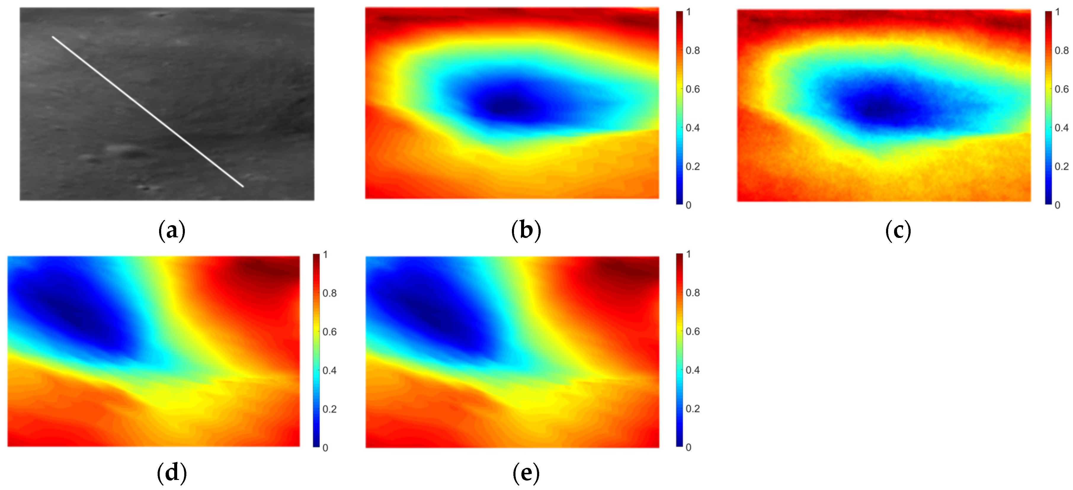
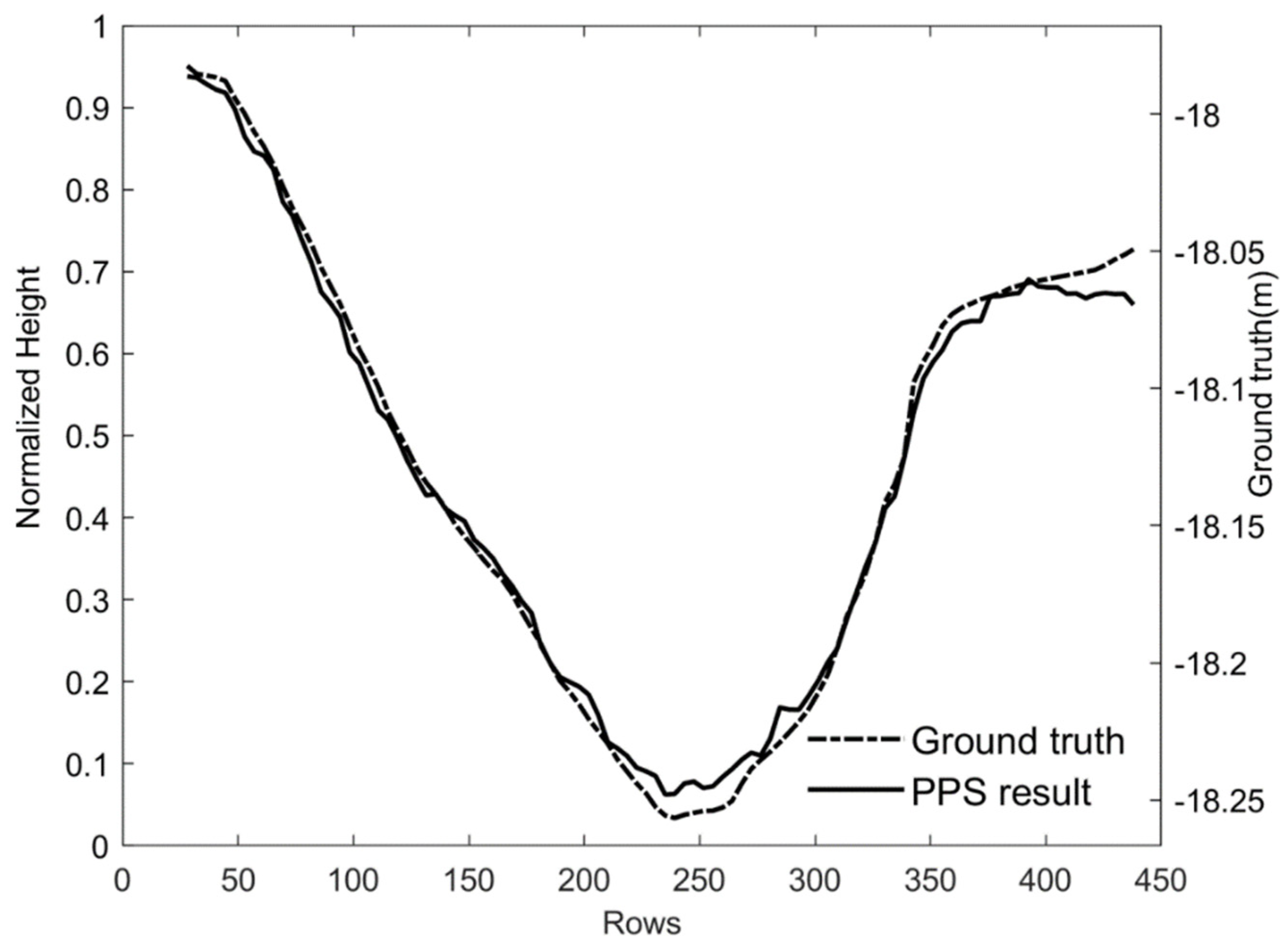
4.2. Experimental Analysis for Simulated Data

The mapping accuracy of the PPS should be investigated. Due to the difficulty of obtaining ground-truth height information of images under different illumination conditions for rover cameras, simulated images are used to validate the effectiveness and the accuracy of the proposed method. The simulated images are generated from digital projection with a virtual camera by using the existing Chang’e-2 DEM and DOM of an area of lunar surface. The resolutions of DOM and DEM are 4.5 m, and the vertical accuracy of the DEM is tens of centimeters. As the resolution of DEM generated by rover image is 0.02 m [8], in order to obtain the corresponding simulated rover images, DEM and DOM have been considered as 0.02 m with 1400 × 1000 pixels, as shown in Figure 4.

Given the interior and exterior orientation parameters, pixel size, image size, and illumination conditions for the virtual camera, the corresponding simulated images can be generated using back projection techniques based on the rigorous sensor model, i.e., the collinearity equations. The distortion parameters are assumed to be equal to zero, while the exterior orientation parameters of different images are defined differently. Height values from the DEM are used as ground truth. Based on the illumination conditions, Chang’e-2 DEM and DOM, ambient lighting, diffuse lighting, and specular lighting vectors are calculated, respectively, and Lommel–Seeliger model is used to derive the simulated images. Figure 5 shows three simulated images under different illumination conditions.

Table 1. Illumination conditions of the simulated images.

Image ID	Solar Azimuth Angle (°)	Solar Elevation Angle (°)	Approximated Phase Angle (°)
Figure 5b	90	55	107.5
Figure 5c	90	60	103.3
Figure 5d	90	65	99.0

lists illumination conditions of the simulated images. There are tens of small craters in the image, and a larger crater is clear on the right side. As the field of view (FOV) of the camera is limited, the craters show different scales, specifically the crater in the red rectangular of Figure 5a corresponds to the marked crater in Figure 5c, other craters in the distance have been compressed due to the principle of the pin-hole model. In order to verify the method efficiently, there are no shadows in the simulated images.

Figure 6 shows height map of ground truth and estimated results using PPS, PSPP [57], and PSOP methods. After replacing the normalized surface normal (12) with Equations (14) and (1), respectively, the height gradient (p, q) can be calculated, PSPP and PSOP results are generated from the corresponding height gradient (p, q). It is noted that the height values have been normalized to the same scale [0, 1]. As illustrated in Figure 6b, the height of large craters at the right side and the upper left corner of the image are recovered distinctly. Small scale features, such as several small crater on the upper right corner of image, are also recovered. Furthermore, the height changes between some small craters and surrounding area are obvious. For comparison purposes, PSPP and PSOP results are shown in Figure 6c,d. Although PSPP is based on the perspective projection model with identity rotation matrix, the errors of the PSPP result are very large and similar with that of PSOP. These two results deviate from the ground truth. For example, the large craters at the right side and the upper left corner of the image are distorted, and the ejecta blankets are not recovered. Two regions of interest (ROI) are chosen to compare in detail. ROI 1 is located at the upper left corner of the image, it includes a large crater and several small craters. ROI 2 includes the largest crater in the image, the height values change greatly in this region.

The enlarged view of ROI 1 and the height maps of ground truth and the three methods are shown in Figure 7. The height distribution of PPS result is the same as the ground truth. As shown in Figure 7c, the details of the terrain are obtained, e.g., both the ejecta blankets of two big craters and the rim of the small crater has been correctly recovered using PPS method. As shown in Figure 7d,e, the resultant distributions of elevations are different from the ground truth, regions of two craters in Figure 7c are merged into a larger region, and the details of craters cannot be recognized. The differences are caused by the lack of interior and exterior elements. A profile along the diagonal direction in Figure 7a is extracted and shown in Figure 8, the left y-axis is the normalized height, the right y-axis represents the real height. The height of virtual camera is −16.5 m, the axis of elevation points down. As Figure 8 shows, the PPS results of ROI 1 extract the height change of the craters, and the height profile of the PPS results is well consistent with the ground truth. Converting to real height difference, the reconstruction errors are at millimeter to centimeter level. It is noted that differences in PPS result at the beginning part is greater than the end part. The larger errors may be due to the elevation of the craters located at the top of the image change frequently, the small error of the height gradients in this area may affect the integrated results.

For ROI 2, Figure 9a shows a large crater where there is significant height difference between the rim and bottom, Figure 9c shows the details of the whole crater, including the bottom, wall, and ejecta blanket, has been well recovered using PPS method. Although there are several small craters located at the bottom side of the image, the height difference is small, the ground truth in Figure 9b does not show the corresponding terrain detail, and so does the PPS result. Figure 9d,e show a distorted part of a crater, which is different from the ground-truth shown in Figure 9b, and the ejecta blanket is not correctly recovered. This is caused by the ignorance of rotation matrix in the PSPP and PSOP methods. Figure 10 shows the height profiles along the white line in Figure 9a, which demonstrate a significant decrease along the wall of crater. According to the ground truth, the depth of the big crater is about 0.2 m. It is observed that the errors of PPS result are very small at millimeter to centimeter level. It seems the bottom of the crater shows relatively larger deviations, which needs further investigation.

To quantitatively evaluate the three methods for the simulated image, MEANN are obtained from these results. As the elevation coordinates of PSPP and PSOP are different from ground truth, the heights cannot be transferred and compared directly, NFD is only calculated for PPS. As the normal vectors of three methods correspond to different object coordinates, it is worth noting that the normal vectors of PSPP and PSOP were multiplied by rotation matrix before calculating the corresponding MEANN.

From the quantitative results of

Table 2. Quantitative measures of three methods for the simulated images.

	Methods	MEANN (°)	NFD
ROI 1	PPS	0.494	0.003
	PSPP	59.799	-
	PSOP	60.065	-
ROI 2	PPS	0.734	0.092
	PSPP	59.998	-
	PSOP	59.855	-
whole image	PPS	0.324	0.042
	PSPP	59.963	-
	PSOP	59.960	-

, both PSPP and PSOP methods show large errors, which are around 60°. The MEANN are similar for ROI 1 and ROI 2. For the whole image, the values of MEANN are between that of ROI 1 and ROI 2. Although PSPP uses the identity matrix, it does not show notable better performance than PSOP when the images are obtained with large pitch angles.

MEANN values of PPS for two regions are less than 1°, NFD of ROI 1 is less than that of ROI 2. Since ROI 1 and ROI 2 represent two areas with large slope, the elevation of other areas change less, the results of whole image are mainly affected by the two regions. The PPS quantitative measures of whole image is larger than that of ROI 1 and smaller than that of ROI 2. For the whole image, MEANN of PPS is 0.324°, and NFD is 0.042, which show good performance of the PPS method.

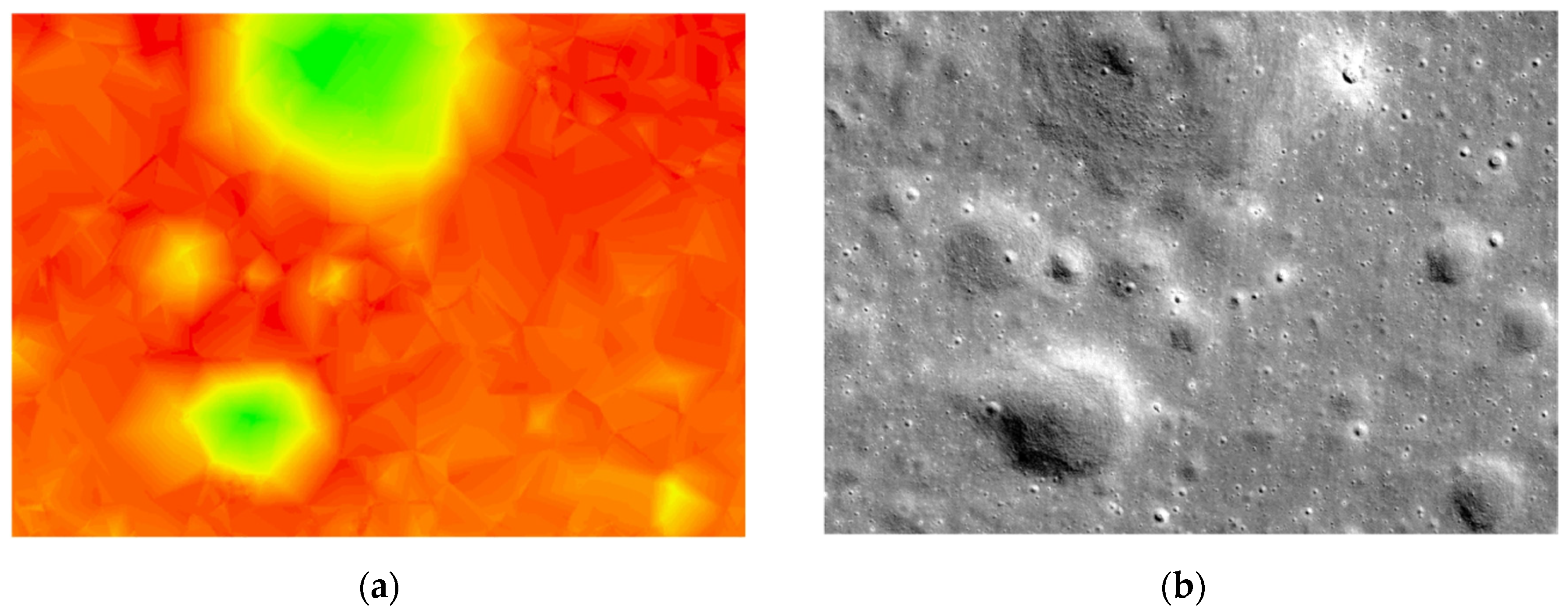
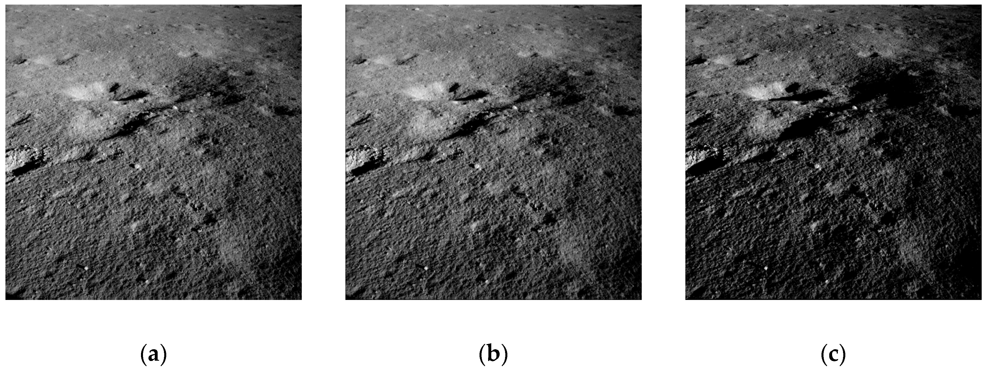
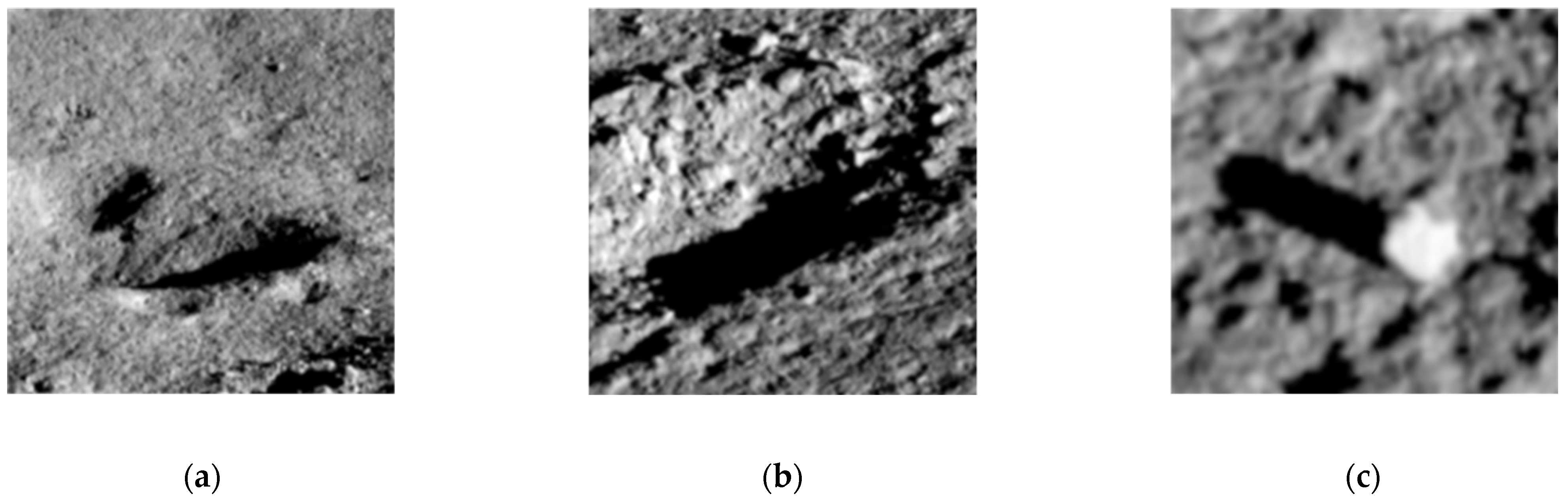
4.3. Experimental Analysis for Yutu-2 Data

Yutu-2 rover of Chang’e-4 mission carries three pairs of stereo cameras: Pancam, Navcam, and Hazcam [8]. The Navcam is mounted on the mast of the rover, and is mainly used for navigation of the rover.

Table 3. Geometric parameters of Chang’e-4 Navcam stereo cameras.

Stereo baseline	0.27 m
Focal length	1189 pixels
Pixel size	1024 × 1024
FOV	46.4° × 46.4°

lists the geometric parameters of Navcam stereo cameras. Normally, at each waypoint, the rover takes a sequence of Navcam images at every 20° in yaw direction at a fixed pitch angle [5]. As a special experiment, the rover obtained 3 pair of Navcam images at a fixed waypoint under different illuminations on 7 August 2019, within the 8th lunar day of the mission. Figure 11 shows the three left images used in our experiment. Their imaging conditions are summarized in

Table 4. Illumination conditions of the images used in the experiment.

Image ID	Solar Azimuth Angle (°)	Solar Elevation Angle (°)	Approximated Phase Angle (°)
94741	−70.8	17	37.7
94914	−71.8	16.2	38.6
95633	−77.1	11.4	44.1

. It can be observed that image tones and shadows change with the change of illumination conditions. The shadow regions are common on the rover images due to complex interactions of geometry and illumination. Figure 12 shows shadows inside craters or behind a boulder.

In order to detect shadow pixels in the images, each image is segmented using 2D Otsu thresholding method [72], which extends the Otsu method from one-dimensional to two-dimensional. The 2D Otsu algorithm is based on two-dimensional gray histogram. It utilizes the gray level of each pixel, as well as the average gray level of pixels in its neighborhood, and performs better than the traditional Otsu’s method in case of low signal-to-noise ratio (SNR). Figure 13a–c show the shadow maps of the three images generated by the 2D OTSU method, the final shadow map is obtained after using union operation of the three shadow maps of (a), (b), and (c). Figure 13d shows the final shadow map used in the experiment. It can be seen that the lower parts of the images are full of shadows. This is due to the solar elevation angles of the three images are all small, 17° or less.

To quantitatively evaluate the accuracy of the PPS method, the semi-global matching (SGM) [38] is used on the first pair of stereo images to achieve height map as ground truth. Semi-global matching is performed to attain the disparity map, where the energy function is built on the determined disparity range of each pixel. The energy function used is as follows

$$E\left(D\right)={\sum }_{p}C\left(p,D_p\right)+{\sum }_{q\in N_P}{P}_{1}T\left[\left|D_p-D_q\right|=1\right]+{\sum }_{q\in N_P}{P}_{2}T[\left|D_p-D_q\right|>1],$$

(35)

where C(p, Dp) is the matching cost of pixel p with disparity Dp, P₁, P₂ represent constant penalty coefficients for all pixels q in the neighborhood of p.

Least squares matching is then performed to attain sub-pixel matching result. After that, 3D coordinates are calculated by space intersection using interior and exterior parameters, finally the height map can be generated.

As Figure 13d shows, although the lower part of image is full of shadows, there exist some continuous non-shaded areas on the upper part that can be used to reconstruct height map using PPS, PSPP and PSOP methods. Figure 14a shows the detail of the upper part image, Figure 14b shows the corresponding shadow map, two regions labelled as 1 and 2 are used to validate PPS method.

Figure 15 shows enlarged views of the area ROI 1 outlined in Figure 14b, the area includes lunar regolith and the rim of a small crater. SGM results and results of three methods have been normalised. As Figure 15b shows, the heights change continuously in a small range, and the rim of the small crater is recovered correctly. The height distribution of PPS result in Figure 15c is similar with that of SGM result, where the upper part is higher than the lower part. Figure 15d,e show SGM and PPS result of ROI 1 with corresponding hillshade map. The rims of three small craters in Figure 15e are clear, and subtle terrain details are displayed. As the boulders are too small, they cannot be recognised in Figure 15d,e. Figure 15f,g represent PSPP and PSOP results. As PSPP and PSOP do not include the rotation matrix, the reconstructed results are inconsistent with the SGM result. The height distributions are similar where the left part is higher than the right part. The elevation axis of Yutu-2 points up, the origin of elevation axis located at the centre of rover body chassis. Figure 15h shows the profile of the boulder marked by the white circle in Figure 15a. Figure 16 shows SGM and PPS results of the profile along the white line in Figure 15a, the left y-axis is the normalized height, the right y-axis represents the real height. According to the SGM result, height range of the test area is about 0.18 m. Most of the normalised height of PPS result is larger than that of SGM result, the trend of the curves is consistent.

Enlarged view of ROI 2 is shown in Figure 17a–c show SGM result and normalised PPS result, respectively. Although there exist some isolated height values in the PPS result, the overall distribution of PPS result is close to that of SGM result, and the lower-right corner of ROI 2 in the crater has the lowest height values. Figure 17d,e show SGM and PPS results of ROI 2 with hillshading effects. Figure 17f,g show PSPP and PSOP results with large deviations, indicating that these two methods are not applicable. Being similar with Figure 15d,e, there is a small rotation angle between the PSPP result and the PSOP result. Figure 17h shows the profile of the boulder marked by the white circle in Figure 17a. The profiles of PPS result and SGM result along the white line are shown in Figure 18. As the white line crosses a part of the small crater, the height values decrease continuously, and the maximum height range is about 0.2m. The PPS result is generally consistent with the SGM results with difference at centimeter level, demonstrating the effectiveness of the PPS method.

Table 5. Quantitative measures of three methods for Yutu-2 images.

	Methods	MEANN (°)	NFD
ROI 1	PPS	8.274	0.336
	PSPP	93.792	-
	PSOP	102.746	-
ROI 2	PPS	9.459	0.386
	PSPP	86.786	-
	PSOP	101.843	-

summarizes the errors of two regions from different methods. The MEANN values of PSPP and PSOP are large, which are almost ten times the result of PPS. For the PPS method, MEANN and NFD of ROI 1 are smaller than those of ROI 2, indicating the method performs better for ROI 1 than for ROI 2, which is in good agreement with the profile maps. Due to the presence of image noises and other errors, the quantitative evaluation values are larger than that of the simulated images.

As rover images are largely oblique, PPS results show higher accuracy than that of PSPP and PSOP. For general cases of PSOP, multiple images under the same viewing geometry with different illumination conditions are available, and the DEM is unknown. To further compare PPS with PSOP, three orthorectified images are generated from corresponding images with mean elevation value. Height map is generated using PSOP based on these orthorectified images. The PPS height result is transformed from image space into object space in order for comparison with the PSOP result. The steps of PPS DEM generation is as follows: (1) After SGM matching, the object coordinates of each point can be obtained; (2) The height value is replaced with PPS normalized result; (3) DEM with 0.005 m resolution is generated using Kriging interpolation method.

Figure 19 shows orthorectified images of ROI 1. Figure 20 shows the normalized DEM from SGM (a), normalized DEM from PPS (b), and PSOP result based on orthorectified images. As Figure 20b shows, the height distribution is similar with that of Figure 19a, most of the rim of small crater is reconstructed. The upper part of Figure 20c is lower than that of Figure 20a, the rim of small crater is not reconstructed completely.

Following the same procedure, the orthorectified images of ROI 2 is shown in Figure 21. Figure 22 shows the normalized DEMs of three methods of ROI 2. The overall height distribution of Figure 22b is close to that of SGM interpolation result, the coverage of crater is also similar. As shown in Figure 22c, the left part of reconstructed result is lower than that of Figure 22a. Using the SGM result as a reference, the visual comparison results in Figure 20 and Figure 22 indicate that PPS result is generally better that that of PSOP with orthorectified images.

As the height values are all normalized, statistical measures including NIQE [73] and BRISQUE [74,75] were adopted to evaluate three DEM results. NIQE compares image to a default model computed from images of natural scenes. A smaller score indicates better perceptual quality. The BRISQUE model is based on a pretrained imaging model, the lower values represent better quality.

Table 6. Quantitative measures of DEMs by three methods for Yutu-2 images.

	Methods	NIQE	BRISQUE
ROI 1	SGM	11.15	45.41
	PPS	10.81	45.26
	PSOP for orthorectified images	11.24	46.15
ROI 2	SGM	7.819	47.47
	PPS	7.540	47.37
	PSOP for orthorectified images	8.230	48.31

summarizes quantitative measures of DEMs generated by three methods. For PPS result, the NIQE and BRISUE values are the smallest for ROI 1 and ROI 2. These statistical measures also demonstrate that the quality of the DEM derived from the PPS method is better than that derived from PSOP with orthorectified images. However, if the DEM of stereo images are available, the DEM result based on photoclinometry will show great improvement [40].

5. Conclusions and Discussion

This paper proposes a photogrammetric-photometric stereo (PPS) method to recover the height map from multiple rove images taken by a single camera under the same viewing geometry with changing illumination conditions. The new imaging irradiance model is developed based on collinearity equations and lunar reflectance model. The relationship between surface normal and elevation gradients derived in the method is the key to the final estimation of height map. The experimental results of simulated images and actual Yutu-2 rover images show that the proposed PPS method algorithm can reconstruct pixel-level height that preserves terrain details, while the reconstructed height map is consistent with ground truth. The height reconstruction error varies between millimeter to centimeter level. Because of the Navcam images taken at the same waypoint with different illumination conditions is limited, and that the differences of azimuth angles and elevation angles among the experimental images are small, the terrain reconstruction errors of the actual rover images are generally larger that of the simulated images. This implies that the illumination differences of multiple images used in photometric stereo affect the resulting height accuracy.

PSPP and PSOP results show large deviations from the ground truth, and PSPP does not show better performance than PSOP when the images are obtained with large pitch angles. The MEANN measure of PSPP and PSOP results are almost ten times larger than the result of PPS, indicating the importance of incorporating the rotation matrix in photogrammetric-photometric stereo (PPS) model. In other words, the traditional PSPP and PSOP methods are not appropriate in rover image based topographic mapping. Further comparisons show that the quality of DEM derived from PPS method is better than that derived from PSOP with orthorectified images.

In this research, Lommel–Seeliger model is used without considering the phase angle and photometric properties of the lunar surface. Other reflectance models, such as lunar–Lambert and Hapke model can also be used for gradient calculation. These can be investigated and compared in future research.

The proposed approach enriches the photometric stereo theory, and extends the orthographic and perspective projection with identity matrix in classical photometric stereo to general cases in close-range topographic mapping. It can also be used for surface reconstruction of other planets with the corresponding reflectance model. In the near future, we will also validate the performance of the model using more ground-based images. Moreover, as the reconstructed height map are of relative height values, further study can be performed by integrating stereo matching and PPS method to improve the details and accuracy of rover image based topographic mapping.

References

1. Di, K.; Zhu, M.; Yue, Z.; Lin, Y.; Wan, W.; Liu, Z.; Gou, S.; Liu, B.; Pang, M.; Wang, Y.; et al. Topographic Evolution of Von Kármán Crater Revealed by the Lunar Rover Yutu. Geophys. Res. Lett. 2019, 46, 12764–12770. [Google Scholar] [CrossRef]
2. Qiao, L.; Ling, Z.; Fu, X.; Li, B. Geological characterization of the Chang’e-4 landing area on the lunar farside. Icarus 2019, 333, 37–51. [Google Scholar] [CrossRef]
3. Yue, Z.; Di, K.; Liu, Z.; Michael, G.; Jia, M.; Xin, X.; Liu, B.; Peng, M.; Liu, J. Lunar regolith thickness deduced from concentric craters in the CE-5 landing area. Icarus 2019, 329, 46–54. [Google Scholar] [CrossRef]
4. Liu, Z.; Di, K.; Peng, M.; Wan, W.; Liu, B.; Li, L.; Yu, T.; Wang, B.; Zhou, J.; Chen, H. High precision landing site mapping and rover localization for Chang’e-3 mission. Sci. China Ser. G Phys. Mech. Astron. 2015, 58, 1–11. [Google Scholar] [CrossRef]
5. Liu, Z.; Di, K.; Li, J.; Xie, J.; Cui, X.; Xi, L.; Wan, W.; Peng, M.; Liu, B.; Wang, Y.; et al. Landing site topographic mapping and rover localization for Chang’e-4 mission. Sci. China Inf. Sci. 2020, 63, 1–12. [Google Scholar] [CrossRef] [Green Version]
6. Di, K.; Liu, Z.; Liu, B.; Wan, W.; Peng, M.; Wang, Y.; Gou, S.; Yue, Z.; Xin, X.; Jia, M.; et al. Chang’e-4 lander localization based on multi-source data. J. Remote Sens. 2019, 23, 177–184. [Google Scholar]
7. Di, K.; Liu, Z.; Wan, W.; Peng, M.; Liu, B.; Wang, Y.; Gou, S.; Yue, Z. Geospatial technologies for Chang’e-3 and Chang’e-4 lunar rover missions. Geo-Spat. Inf. Sci. 2020, 23, 87–97. [Google Scholar] [CrossRef]
8. Wang, Y.; Wan, W.; Gou, S.; Peng, M.; Liu, Z.; Di, K.; Li, L.; Yu, T.; Wang, J.; Cheng, X. Vision-Based Decision Support for Rover Path Planning in the Chang’e-4 Mission. Remote Sens. 2020, 12, 624. [Google Scholar] [CrossRef] [Green Version]
9. Peng, M.; Wan, W.; Wu, K.; Liu, Z.; Li, L.; Di, K.; Li, L.; Miao, Y.; Zhang, L. Topographic mapping capability analysis of Chang’e-3 Navcam stereo images and three-dimensional terrain reconstruction for mission operations. J. Remote Sens. 2014, 18, 995–1002. [Google Scholar]
10. Jia, Y.; Zou, Y.; Ping, J.; Xue, C.; Yan, J.; Ning, Y. The scientific objectives and payloads of Chang’E−4 mission. Planet. Space Sci. 2018, 162, 207–215. [Google Scholar] [CrossRef]
11. Horn, B.K. Understanding image intensities. Artif. Intell. 1977, 8, 201–231. [Google Scholar] [CrossRef] [Green Version]
12. Horn, B.K.P. Height and gradient from shading. Int. J. Comput. Vis. 1990, 5, 37–75. [Google Scholar] [CrossRef]
13. Woodham, R.J. Photometric Method For Determining Surface Orientation from Multiple Images. Opt. Eng. 1980, 19, 191139. [Google Scholar] [CrossRef]
14. Lohse, V.; Heipke, C. Multi-image shape-from-shading: Derivation of planetary digital terrain models using clementine images. Int. Arch. Photogramm. Rem. Sens. 2004, 35, 828–833. [Google Scholar]
15. Lohse, V.; Heipke, C.; Kirk, R.L. Derivation of planetary topography using multi-image shape-from-shading. Planet. Space Sci. 2006, 54, 661–674. [Google Scholar] [CrossRef]
16. Grumpe, A.; Belkhir, F.; Wöhler, C. Construction of lunar DEMs based on reflectance modelling. Adv. Space Res. 2014, 53, 1735–1767. [Google Scholar] [CrossRef]
17. Wu, B.; Liu, W.C.; Grumpe, A.; Wöhler, C. Construction of pixel-level resolution DEMs from monocular images by shape and albedo from shading constrained with low-resolution DEM. ISPRS J. Photogramm. Remote Sens. 2018, 140, 3–19. [Google Scholar] [CrossRef]
18. Alexandrov, O.; Beyer, R.A. Multiview Shape-From-Shading for Planetary Images. Earth Space Sci. 2018, 5, 652–666. [Google Scholar] [CrossRef]
19. Liu, W.C.; Wu, B. An integrated photogrammetric and photoclinometric approach for illumination-invariant pixel-resolution 3D mapping of the lunar surface. ISPRS J. Photogramm. Remote Sens. 2020, 159, 153–168. [Google Scholar] [CrossRef]
20. Burns, K.N.; Speyerer, E.J.; Robinson, M.S.; Tran, T.; Rosiek, M.R.; Archinal, B.A.; Howington-Kraus, E. Digital elevation models and derived products from LROC NAC stereo ob-servations. ISPRS-International Archives of the Photogrammetry. Remote Sens. Spat. Inf. Sci. 2012, 39, 483–488. [Google Scholar]
21. Shean, D.; Alexandrov, O.; Moratto, Z.M.; Smith, B.E.; Joughin, I.; Porter, C.; Morin, P. An automated, open-source pipeline for mass production of digital elevation models (DEMs) from very-high-resolution commercial stereo satellite imagery. ISPRS J. Photogramm. Remote Sens. 2016, 116, 101–117. [Google Scholar] [CrossRef] [Green Version]
22. DeVenecia, K.; Walker, A.S.; Zhang, B. New approaches to generating and processing high resolution elevation data with imagery. In Proceedings of the Photogrammetric Week, Heidelberg, Germany, 3–9 September 2007; pp. 1442–1448. [Google Scholar]
23. Re, C.; Cremonese, G.; Dall’Asta, E.; Forlani, G.; Naletto, G.; Roncella, R. Performance evaluation of DTM area-based matching reconstruction of Moon and Mars. In Proceedings of the SPIE Remote Sensing, Edinburgh, UK, 24–27 September 2012; p. 8537. [Google Scholar]
24. Hu, H.; Wu, B. Planetary3d: A photogrammetric tool for 3d topographic mapping of planetary bodies. ISPRS Ann. Photogramm. Remote Sens. Spat. Inf. Sci. 2019, IV-2/W5, 519–526. [Google Scholar] [CrossRef] [Green Version]
25. Haruyama, J.; Ohtake, M.; Matsunaga, T.; Morota, T.; Honda, C.; Yokota, Y.; Ogawa, Y. Selene (Kaguya) terrain camera observation results of nominal mission period. In Proceedings of the 40th Lunar and Planetary Science Conference, Woodlands, TX, USA, 23–27 March 2009. [Google Scholar]
26. Tran, T.; Rosiek, M.R.; Beyer, R.A.; Mattson, S.; Howington-Kraus, E.; Robinson, M.S.; Archinal, B.A.; Edmunson, K.; Harbour, D.; Anderson, E. Generating digital terrain models using LROC NAC images. In Proceedings of the ASPRS/CaGIS 2010 Fall Specialty Conference, Orlando, FL, USA, 15–19 November 2010. [Google Scholar]
27. Di, K.; Liu, Y.; Liu, B.; Peng, M.; Hu, W. A self calibration bundle adjustment method for photogrammetric processing of Chang’E-2 stereo lunar imager. IEEE Trans. Geosci. Remote Sens. 2014, 52, 5432–5442. [Google Scholar]
28. Wu, B.; Guo, J.; Zhang, Y.; King, B.; Li, Z.; Chen, Y. Integration of Chang’E-1 Imagery and Laser Altimeter Data for Precision Lunar Topographic Modeling. IEEE Trans. Geosci. Remote Sens. 2011, 49, 4889–4903. [Google Scholar] [CrossRef]
29. Wu, B.; Hu, H.; Guo, J. Integration of Chang’E-2 imagery and LRO laser altimeter data with a combined block adjustment for precision lunar topographic modeling. Earth Planet. Sci. Lett. 2014, 391, 1–15. [Google Scholar] [CrossRef]
30. Liu, Y.; Di, K. Evaluation of Rational Function Model for Geometric Modeling of Chang’e-1 CCD Images. ISPRS Int. Arch. Photogramm. Remote Sens. Spat. Inf. Sci. 2012, 38, 121–125. [Google Scholar] [CrossRef] [Green Version]
31. Liu, B.; Liu, Y.; Di, K.; Sun, X. Block adjustment of Chang’E-1 images based on rational function model. In Proceedings of the Remote Sensing of the Environment: 18th National Symposium on Remote Sensing of China, Wuhan, China, 20–23 October 2012; Volume 9158, p. 91580G. [Google Scholar]
32. Liu, B.; Xu, B.; Di, K.; Jia, M. A solution to low RFM fitting precision of planetary orbiter images caused by exposure time changing. In Proceedings of the International Archives of the Photogrammetry, Remote Sensing and Spatial Information Sciences, Prague, Czech Republic, 12–19 July 2016; pp. 441–448. [Google Scholar]
33. Hu, H.; Wu, B. Block adjustment and coupled epipolar rectification of LROC NAC images for precision lunar topographic mapping. Planet. Space Sci. 2018, 160, 26–38. [Google Scholar] [CrossRef]
34. Liu, B.; Jia, M.; Di, K.; Oberst, J.; Xu, B.; Wan, W. Geopositioning precision analysis of multiple image triangulation using LROC NAC lunar images. Planet. Space Sci. 2018, 162, 20–30. [Google Scholar] [CrossRef]
35. Wu, B.; Zeng, H.; Hu, H. Illumination invariant feature point matching for high-resolution planetary remote sensing images. Planet. Space Sci. 2018, 152, 45–54. [Google Scholar] [CrossRef]
36. Furukawa, Y.; Ponce, J. Accurate, Dense, and Robust Multi-View Stereopsis. IEEE Trans. Pattern Anal. Mach. Intell. 2007, 32, 1362–1376. [Google Scholar] [CrossRef]
37. Wu, B.; Zhang, Y.; Zhu, Q. Integrated point and edge matching on poor textural images constrained by self-adaptive trian-gulations. ISPRS J. Photogramm. Remote Sens. 2012, 68, 40–55. [Google Scholar] [CrossRef]
38. Hirschmuller, H. Accurate and Efficient Stereo Processing by Semi-Global Matching and Mutual Information. IEEE Trans. Pattern Anal. Mach. Intell. 2005, 30, 807–814. [Google Scholar] [CrossRef]
39. Hu, H.; Chen, C.; Wu, B.; Yang, X.; Zhu, Q.; Ding, Y. Texture-Aware Dense Image Matching using Ternary Census Transform. ISPRS Ann. Photogramm. Remote Sens. Spat. Inf. Sci. 2016, 3, 59–66. [Google Scholar] [CrossRef] [Green Version]
40. Wu, B.; Li, Y.; Liu, W.C.; Wang, Y.; Li, F.; Zhao, Y.; Zhang, H. Centimeter-resolution topographic modeling and fine-scale analysis of craters and rocks at the Chang’E-4 landing site. Earth Planet. Sci. Lett. 2021, 553, 116666. [Google Scholar] [CrossRef]
41. Taguchi, M.; Funabashi, G.; Watanabe, S.; Fukunushi, H. Lunar albedo at hydrogen Lyman α by the NOZOMI/UVS. J. Earth Planets Space 2000, 52, 645–647. [Google Scholar] [CrossRef] [Green Version]
42. Kirk, R.L. A Fast Finite-element Algorithm for Two-dimensional Photoclinometry. Ph.D. Thesis, Division of Geological and Planetary Sciences, California Institute of Technology, Pasadena, CA, USA, 1987; pp. 165–258. [Google Scholar]
43. Kirk, R.L.; Barrett, J.M.; Soderblom, L.A. Photoclinometry Made Simple. In Proceedings of the ISPRS Commission IV, Working Group IV/9 2003, ‘‘Advances in Planetary Mapping” Workshop, Houston, TX, USA, 22 March 2003. [Google Scholar]
44. O’Hara, R.; Barnes, D. A new shape from shading technique with application to Mars Express HRSC images. ISPRS J. Photogramm. Remote Sens. 2012, 67, 27–34. [Google Scholar] [CrossRef]
45. Kirk, R.L.; Howington-Kraus, E.; Redding, B.; Galuszka, D.; Hare, T.M.; Archinal, B.A.; Soderblom, L.A.; Barret, J.A. High-resolution topomapping of candidate MER landing sites with Mars orbiter camera narrow-angle images. J. Geophys. Res. 2003, 108, 8088. [Google Scholar] [CrossRef]
46. Beyer, R.A.; Kirk, R.L. Meter-scale slopes of candidate MSL landing sites from point photoclinometry. Space Sci. Rev. 2012, 170, 775–791. [Google Scholar] [CrossRef]
47. Wu, B.; Li, F.; Hu, H.; Zhao, Y.; Wang, Y.; Xiao, P.; Li, Y.; Liu, W.C.; Chen, L.; Ge, X.; et al. Topographic and Geomorphological Mapping and Analysis of the Chang’E-4 Landing Site on the Far Side of the Moon. Photogramm. Eng. Remote Sens. 2020, 86, 247–258. [Google Scholar] [CrossRef]
48. Wöhler, C.; Grumpe, A.; Berezhnoy, A.; Bhatt, M.U.; Mall, U. Integrated topographic, photometric and spectral analysis of the lunar surface: Application to impact melt flows and ponds. Icarus 2014, 235, 86–122. [Google Scholar] [CrossRef]
49. Gao, Y.; Spiteri, C.; Li, C.; Zheng, Y.C. Lunar soil strength estimation based on Chang’E-3 images. Adv. Space Res. 2016, 58, 1893–1899. [Google Scholar] [CrossRef] [Green Version]
50. Ding, C.; Xiao, Z.; Wu, B.; Li, Y.; Prieur, N.C.; Cai, Y.; Su, Y.; Cui, J. Fragments delivered by secondary craters at the Chang’e 4 landing site. Geophys. Res. Lett. 2020, 47, e2020GL087361. [Google Scholar] [CrossRef]
51. Jiang, C.; Douté, S.; Luo, B.; Zhang, L. Fusion of photogrammetric and photoclinometric information for high-resolution DEMs from Mars in-orbit imagery. ISPRS J. Photogramm. Remote Sens. 2017, 130, 418–430. [Google Scholar] [CrossRef]
52. Tenthoff, M.; Wohlfarth, K.; Wöhler, C. High Resolution Digital Terrain Models of Mercury. Remote Sens. 2020, 12, 3989. [Google Scholar] [CrossRef]
53. Ackermann, J.; Langguth, F.; Fuhrmann, S.; Goesele, M. Photometric stereo for outdoor webcams. In Proceedings of the IEEE Conference on Computer Vision and Pattern Recognition, Providence, RI, USA, 16–21 June 2012; pp. 262–269. [Google Scholar]
54. Liu, W.C.; Wu, B.; Wöhler, C. Effects of illumination differences on photometric stereo shape-and-albedo-from-shading for precision lunar surface reconstruction. ISPRS J. Photogramm. Rem. Sens. 2018, 136, 58–72. [Google Scholar]
55. Herbort, S.; Wöhler, C. An introduction to image-based 3D surface reconstruction and a survey of photometric stereo methods. 3D Res. 2011, 2, 1–17. [Google Scholar] [CrossRef]
56. Ackermann, J.; Goesele, M. A survey of photometric stereo techniques. Found. Trends Comput. Graph. Vis. 2015, 9, 149–254. [Google Scholar] [CrossRef]
57. Tankus, A.; Kiryati, N. Photometric stereo under perspective projection. In Proceedings of the Tenth IEEE International Conference on Computer Vision (ICCV’05), Beijing, China, 17–21 October 2005; pp. 611–616. [Google Scholar]
58. Argyriou, V.; Petrou, M. Photometric Stereo: An Overview. Adv. Imaging Electron Phys. 2009, 156, 1–54. [Google Scholar]
59. Tankus, A.; Sochen, N.; Yeshurun, Y. Shape-from-shading under perspective projection. Int. J. Comput. Vis. 2005, 63, 21–43. [Google Scholar] [CrossRef]
60. Hapke, B. Theory of Reflectance and Emittance Spectroscopy; Cambridge University Press: Cambridge, UK, 2012; ISBN 978-1-139-21750-7. [Google Scholar]
61. McEwen, A.S. Photometric functions for photoclinometry and other applications. Icarus 1991, 92, 298–311. [Google Scholar] [CrossRef]
62. Hapke, B. Bidirectional reflectance spectroscopy: The coherent backscatter opposition effect and anisotropic scattering. Icarus 2002, 157, 523–534. [Google Scholar] [CrossRef] [Green Version]
63. Besse, S.; Sunshine, J.; Staid, M.; Boardman, J.; Pieters, C.; Guasqui, P.; Maralet, E.; McLaughlin, S.; Yokota, Y.; Li, J.-Y. A visible and near-infrared photometric correction for Moon Mineralogy Mapper (M3). Icarus 2013, 222, 229–242. [Google Scholar] [CrossRef]
64. Hillier, J.K.; Buratti, B.J.; Hill, K. Multispectral photometry of the Moon and absolute calibration of the Clementine UV/Vis camera. Icarus 1999, 141, 205–225. [Google Scholar] [CrossRef]
65. Sato, H.; Denevi, B.W.; Robinson, M.S.; Boyd, A.; Hapke, B.W.; McEwen, A.S.; Speyerer, E.J. Photometric normalization of LROC WAC global color mosaic. Lunar Planet. Sci. 2001, XLII, 636. [Google Scholar]
66. Wu, Y.; Besse, S.; Li, J.Y.; Combe, J.P.; Wang, Z.; Zhou, X.; Wang, C. Photometric correction and in-flight calibration of Chang’E-1 Interference Imaging Spectrometer (IIM) data. Icarus 2013, 222, 283–295. [Google Scholar] [CrossRef]
67. Bondarenko, N.V.; Dulova, I.A.; Kornienko, Y.V. Photometric Functions and the Improved Photoclinometry Method: Mature Lunar Mare Surfaces. In Proceedings of the Lunar and Planetary Science Conference, The Woodlands, TX, USA, 16–20 March 2020; p. 1845. [Google Scholar]
68. Lin, H.; Yang, Y.; Lin, Y.; Liu, Y.; Wei, Y.; Li, S.; Hu, S.; Yang, W.; Wan, W.; Xu, R.; et al. Photometric properties of lunar regolith revealed by the Yutu-2 rover. Astron. Astrophys. 2020, 638, A35. [Google Scholar] [CrossRef]
69. Gill, P.E.; Murray, W. Algorithms for the solution of the nonlinear least-squares problem. SIAM J. Numer. Anal. 1978, 15, 977–992. [Google Scholar] [CrossRef]
70. Harker, M.; O’Leary, P. Least squares surface reconstruction from gradients: Direct algebraic methods with spectral, Tikhonov, and constrained regularization. In Proceedings of the IEEE Computer Vision Pattern Recognition, Colorado Springs, CO, USA, 20–25 June 2011; pp. 2529–2536. [Google Scholar]
71. Quéau, Y.; Lauze, F.; Durou, J.D. Solving uncalibrated photometric stereo using total variation. J. Math. Imaging Vis. 2015, 52, 87–107. [Google Scholar] [CrossRef] [Green Version]
72. Sha, C.; Hou, J.; Cui, H. A robust 2D Otsu’s thresholding method in image segmentation. J. Vis. Commun. Image Represent. 2016, 41, 339–351. [Google Scholar] [CrossRef]
73. Mittal, A.; Soundararajan, R.; Bovik, A.C. Making a Completely Blind Image Quality Analyzer. IEEE Signal Process. Lett. 2013, 3, 209–212. [Google Scholar] [CrossRef]
74. Mittal, A.; Moorthy, A.K.; Bovik, A.C. No-Reference Image Quality Assessment in the Spatial Domain. IEEE Trans. Image Process. 2012, 21, 4695–4708. [Google Scholar] [CrossRef] [PubMed]
75. Mittal, A.; Moorthy, A.K.; Bovik, A.C. Referenceless Image Spatial Quality Evaluation Engine. In Proceedings of the 45th Asilomar Conference on Signals, Systems and Computers, Pacific Grove, CA, USA, 1–4 November 2011. [Google Scholar]
Figure 1. Framework of photogrammetric-photometric stereo (PPS) method.
Remotesensing 13 02975 g001
Figure 2. Illustration of rover image formation.
Remotesensing 13 02975 g002
Figure 3. Schematic representation of different imaging conditions (a) image and object coordinates for photometric stereo under orthographic projection (PSOP), (b) image and object coordinates for photometric stereo under perspective projection with identity matrix (PSPP), (c) image and object coordinates for PPS.
Remotesensing 13 02975 g003
Figure 4. (a) DEM and (b) DOM for rover image simulation.
Remotesensing 13 02975 g004
Figure 5. Simulated images under different lighting conditions (a) simulate image of solar azimuth angle 90°and elevation angle 55° (b) simulate image of solar azimuth angle 90°and elevation angle 60° (c) simulate image of solar azimuth angle 90°and elevation angle 65° (d).
Remotesensing 13 02975 g005
Figure 6. Height map of ground truth and results of three methods (a) Height map of ground truth, (b) PPS result, (c) PSPP result, (d) PSOP result.
Remotesensing 13 02975 g006
Figure 7. ROI 1 and reconstruction results of the three methods (a) Enlarged view of region 1, (b) ground truth, (c) PPS result, (d) PSPP result, (e) PSOP result.
Remotesensing 13 02975 g007
Figure 8. Height profile of ROI 1 in simulated imagery.
Remotesensing 13 02975 g008
Figure 9. ROI 2 and reconstruction results of the three methods (a) Enlarged view of region 2, (b) ground truth (c) PPS result, (d) PSPP result, (e) PSOP result.
Remotesensing 13 02975 g009
Figure 10. Height profile of ROI 2 in simulated imagery.
Remotesensing 13 02975 g010
Figure 11. Navcam images of the left camera under different illumination conditions (a) 94741, (b) 94914, (c) 95633.
Remotesensing 13 02975 g011
Figure 12. Examples of shadows (a) shadow inside two craters, (b) shadow inside a crater, (c) shadow behind a boulder.
Remotesensing 13 02975 g012
Figure 13. Shadow maps (a) Shadow map of image 94741, (b) Shadow map of image 94914, (c) Shadow map of image 95633, (d) Final shadow map.
Remotesensing 13 02975 g013
Figure 14. (a) Two sub-regions of the image, (b) Shadow map.
Remotesensing 13 02975 g014
Figure 15. ROI 1 and reconstruction results of the three methods (a) ROI 1 image, (b) SGM result, (c) PPS result, (d) shaded SGM result, (e) shaded PPS result, (f) PSPP result, (g) PSOP result, (h) Profile of the boulder (marked by the white circle in (a)) from PPS result.
Remotesensing 13 02975 g015
Figure 16. Height profile of ROI 1 in Yutu-2 rover imagery.
Remotesensing 13 02975 g016
Figure 17. ROI 2 and reconstruction results of the three methods (a) ROI 2 image, (b) SGM result, (c) PPS result, (d) shaded SGM result, (e) shaded PPS result, (f) PSPP result, (g) PSOP result, (h) Profile of the boulder (marked by the white circle in (a)) from PPS result.
Remotesensing 13 02975 g017aRemotesensing 13 02975 g017b
Figure 18. Height profile of ROI 2 in Yutu-2 rover imagery.
Remotesensing 13 02975 g018
Figure 19. Orthorectified images of ROI 1 in Yutu-2 rover imagery (a) ROI 1 of 94741, (b) ROI 1 of 94914, (c) ROI 1 of 95633.
Remotesensing 13 02975 g019
Figure 20. Reconstruction DEM results of ROI1 by three methods (a) SGM interpolation result, (b) PPS interpolation result, (c) PSOP result from orthorectified images.
Remotesensing 13 02975 g020
Figure 21. Orthorectified images of ROI 2 in Yutu-2 rover imagery (a) ROI 2 of 94741, (b) ROI 2 of 94914, (c) ROI 2 of 95633.
Remotesensing 13 02975 g021
Figure 22. Reconstruction results of ROI 2 by three methods (a) SGM interpolation result, (b) PPS interpolation result, (c) PSOP result for orthorectified images.
Remotesensing 13 02975 g022