Coverage and Rainfall Response of Biological Soil Crusts Using Multi-Temporal Sentinel-2 Data in a Central European Temperate Dry Acid Grassland

Abstract

Biological soil crusts (BSCs) are thin microbiological vegetation layers that naturally develop in unfavorable higher plant conditions (i.e., low precipitation rates and high temperatures) in global drylands. They consist of poikilohydric organisms capable of adjusting their metabolic activities depending on the water availability. However, they, and with them, their ecosystem functions, are endangered by climate change and land-use intensification. Remote sensing (RS)-based studies estimated the BSC cover in global drylands through various multispectral indices, and few of them correlated the BSCs’ activity response to rainfall. However, the allocation of BSCs is not limited to drylands only as there are areas beyond where smaller patches have developed under intense human impact and frequent disturbance. Yet, those areas were not addressed in RS-based studies, raising the question of whether the methods developed in extensive drylands can be transferred easily. Our temperate climate study area, the ‘Lieberoser Heide’ in northeastern Germany, is home to the country’s largest BSC-covered area. We applied a Random Forest (RF) classification model incorporating multispectral Sentinel-2 (S2) data, indices derived from them, and topographic information to spatiotemporally map the BSC cover for the first time in Central Europe. We further monitored the BSC response to rainfall events over a period of around five years (June 2015 to end of December 2020). Therefore, we combined datasets of gridded NDVI as a measure of photosynthetic activity with daily precipitation data and conducted a change detection analysis. With an overall accuracy of 98.9%, our classification proved satisfactory. Detected changes in BSC activity between dry and wet conditions were found to be significant. Our study emphasizes a high transferability of established methods from extensive drylands to BSC-covered areas in the temperate climate. Therefore, we consider our study to provide essential impulses so that RS-based biocrust mapping in the future will be applied beyond the global drylands.

1. Introduction

Biological soil crusts (BSCs), or so-called biocrusts, are thin microbiological layers that “result from an intimate association between soil particles, cyanobacteria, algae, microfungi, lichens, and bryophytes, which live within, or immediately on top of the uppermost millimeters of soil” [1]. The presence or absence of water massively influences the physiognomy of BSCs as they consist of poikilohydric organisms, capable of temporally suspending their metabolic activities, such as photosynthesis, when no water is available [2]. These can be recommenced immediately by precipitation events and kept active for up to several days, depending on water availability [2].

BSCs cover around 12% of the Earth’s land surface [3]. While predominantly occurring within arid and semi-arid drylands, BSCs can be found globally throughout different climate zones [4]. They influence ecosystems by limiting the water availability for soil biota, nutrient cycles, and vascular vegetation [5] and highly contribute to the global carbon and nitrogen budgets [5]. Human society benefits from their ecological functions, such as mitigating water and wind erosion [6] and regulating air quality [7]. BSCs are reported as very sensitive to environmental changes, particularly to rising temperature and decreasing humidity [8]. Therefore, they are highly endangered by climate change and land-use intensification, whereby the global BSC cover is expected to decrease by 25 to 40% from 2005 to 2070 [3]. This also implicates the loss of their ecosystem functions. Acquiring more accurate information on their spatiotemporal distribution and dynamic is considered essential for developing sustainable management and protection strategies [1,9,10].

Beyond the arid and semi-arid drylands, a considerable number of drylands featuring BSCs allocates in temperate climates. In Central Europe, they are mainly associated with natural open ecosystems [11,12,13] or disturbed landscapes [14,15]. Dry grasslands with BSCs and soil lichen communities are widespread on quaternary inland dunes deposited during the last glacial time; for example, they are distributed along a belt stretching from the Netherlands, across northern Germany, including Brandenburg, to Poland, and along rivers in southern Germany [14,15,16,17,18]. These habitats are characterized by nutrient-poor soils, dryness, and high solar irradiation [11], allowing colonization by drought-adapted cryptogams without being outcompeted by vascular plants [13]. For instance, in open xeric grasslands, soil lichen and moss communities accompanied by microalgae are especially frequent and influence the ecosystem development [19]. As photoautotroph microbiotic communities, they contribute to carbon accumulation and soil formation of initial sandy soils [15,20]. Furthermore, they change the hydrological properties of the soil surface and alternate sub-critical water hydrophobicity [17,21].

The first use of remote sensing (RS) for BSC-related research dates back to 1986, when optical imagery from the Landsat TM sensor was analyzed [22]. Ever since, studies employed optical and radar RS data from space-borne, airborne, and Unmanned Airborne Vehicle (UAV)-based sensors in different spatial, radiometric, and temporal resolutions [23,24] (Table 1) for classifying and mapping the distribution of BSCs [3,24,25,26,27,28,29,30,31,32,33]. The spectral features of BSCs were identified and characterized using multi-and hyperspectral data to differentiate them from co-occurring land cover types (e.g., bare soil and vascular plants), to distinguish between different crust types, and to assess differences between dry and wet BSCs [33,34,35,36,37,38,39,40,41]. Additionally, RS data was used to model various processes and activities of BSCs related to their ecosystem functions [2,19,42,43,44,45,46,47,48].

The RS-based assessment of BSCs is predominantly based on the optical part of the electromagnetic spectra (Table 1). BSCs show a unique spectral signature that can be utilized via the calculation of spectral indices [31,36,37,38]. The most common one is the Normalized Difference Vegetation Index (NDVI) [49], capable of delineating different vegetation types and their condition. It estimates the amount of green biomass and chlorophyll using the difference in reflectance in the chlorophyll absorption feature at the red and the high reflection in the near-infrared (NIR) spectral domain [49]. With respect to the BSCs, this means that dry and wet conditions must be considered differently, as the spectral reflectance changes with the change in BSC activity and appearance, based on the presence and absence of water. Dry BSCs slightly differ from bare soil, whereas wet BSCs show stronger chlorophyll absorption and higher NIR reflectance resembling vascular plants [33,34,35]. Therefore, the NDVI was commonly applied for assessing the change in metabolic activity of BSCs after precipitation events, as wet biocrusts are reported to show a significantly higher NDVI than dry biocrusts [37,39,40].

Table 1. Remote sensing sensors used for characterizing and mapping biological soil crusts with the corresponding studies’ timeframes and focus areas. MS = multispectral, HS = hyperspectral, UAV = unmanned airborne vehicle, SAR = synthetic aperture radar. * not specified.

Sensor				Timeframes/Temporal Resolution	Focus Areas	References
Platform	Type	Name	Spatial Resolution
Spaceborne	MS	Kompsat-2	1 m	2 images	Niger	[50]
	MS	QuickBird, WorldView-2	2.5 m	2 images	Negev	[51]
	MS	SPOT	20 m	28 images during 2 years	Negev	[45]
	MS	Landsat 4–8	30–75 m	single images, 31 annual composites	Negev, China, Namibia, South Africa	[22,26,27,28,36,48,52]
	MS	Sentinel-2 MSI	10–20 m	single image, 20 images during 2 years, full time series during 2016	China, Negev, Idaho	[28,30,53]
	MS	Meteosat-9 SEVIRI	3 km	Every 15 min during 2 months	Negev	[46]
	MS	ASTER	90 m	“several” images *	Negev	[54]
	MS	MODIS	250 m–1 km	Every 16 days during growing season, every 8 days from 2000 to 2014	Patagonia, China	[55,56]
	SAR	SIR-C	13–30 m	single image	Negev and Sinai	[57]
	SAR	ASAR	- *	15 images during 1.5 years	Negev	[57]
UAV	MS	Ricoh GR II	0.5 cm	single image	Utah	[58]
	MS	DJI X5s	1–3 cm	single images	Hawaii	[59]
	MS	- *	- *	single images	China	[28]
Airborne	HS	AMS	5 m	single images	Australia	[25]
	HS	CASI 1&2	1–1.5 m	single images	Spain, South Africa	[9,10,29,31]
	HS	DAIS	8 m	single images	Negev	[26,36,54]

Table 1. Remote sensing sensors used for characterizing and mapping biological soil crusts with the corresponding studies’ timeframes and focus areas. MS = multispectral, HS = hyperspectral, UAV = unmanned airborne vehicle, SAR = synthetic aperture radar. * not specified.

Sensor				Timeframes/Temporal Resolution	Focus Areas	References
Platform	Type	Name	Spatial Resolution
Spaceborne	MS	Kompsat-2	1 m	2 images	Niger	[50]
	MS	QuickBird, WorldView-2	2.5 m	2 images	Negev	[51]
	MS	SPOT	20 m	28 images during 2 years	Negev	[45]
	MS	Landsat 4–8	30–75 m	single images, 31 annual composites	Negev, China, Namibia, South Africa	[22,26,27,28,36,48,52]
	MS	Sentinel-2 MSI	10–20 m	single image, 20 images during 2 years, full time series during 2016	China, Negev, Idaho	[28,30,53]
	MS	Meteosat-9 SEVIRI	3 km	Every 15 min during 2 months	Negev	[46]
	MS	ASTER	90 m	“several” images *	Negev	[54]
	MS	MODIS	250 m–1 km	Every 16 days during growing season, every 8 days from 2000 to 2014	Patagonia, China	[55,56]
	SAR	SIR-C	13–30 m	single image	Negev and Sinai	[57]
	SAR	ASAR	- *	15 images during 1.5 years	Negev	[57]
UAV	MS	Ricoh GR II	0.5 cm	single image	Utah	[58]
	MS	DJI X5s	1–3 cm	single images	Hawaii	[59]
	MS	- *	- *	single images	China	[28]
Airborne	HS	AMS	5 m	single images	Australia	[25]
	HS	CASI 1&2	1–1.5 m	single images	Spain, South Africa	[9,10,29,31]
	HS	DAIS	8 m	single images	Negev	[26,36,54]

However, in BSC cover estimation and mapping, the NDVI values can be easily confused with other land cover types, such as soils and sparsely woody vegetation, leading to imprecise results [33]. Therefore, other biocrust-specific indices were developed during the last decades. For example, the Crust Index (CI) [26] uses the red and blue spectral bands to detect BSCs based on an increase in reflectivity within the blue spectral domain that is caused by the presence of cyanobacteria. Later, the green and red band combination was found to be very useful, particularly for distinguishing BSCs from vascular plants [28]. The Biological Soil Crust Index (BSCI) [27] utilizes the green, red, and NIR reflectance. It was specifically designed to detect lichen-dominated BSCs [33]. Additionally, the thermal spectra were studied, building on the principle of variations in land surface temperature originating from differences in albedo and absorbance caused by BSCs [60]. The Thermal Crust Index (TCI) [54] was developed for discriminating BSCs from bare sand in deserts and was reported to be particularly powerful when combined with the NDVI and CI [24].

Besides the RS data, topographic information holds enormous potential for supporting soil and vegetation mapping approaches [61,62,63,64,65,66]. Yet, for classifying BSCs, topographic information is not common and has only been discussed recently. For example, topographic attributes (TAs) such as the slope angle, the wetness index, and the solar irradiation [32] were found to control patterns of BSCs and have been successfully employed as environmental covariates (i.e., predictors) in estimating and mapping BSCs [50].

Land cover classification, in general, can be performed using different approaches. Hereby, the ensemble machine learning (ML) algorithm Random Forest (RF) is known for high classification accuracy and providing meaningful results in the context of RS data [67,68]. It is a supervised technique based on reference areas for training and testing the algorithm by defining the characteristics of the classes. It is widely used in RS-based land cover and vegetation mapping applications and was already successfully used to estimate BSC coverage in desert regions in Xingjiang, China [28].

With the launch of the multispectral optical satellite mission Sentinel-2 (S2) within the ESA Copernicus earth observation program, global data of high spatial and temporal resolution is freely available, allowing for continuous global monitoring. The mission is designed to be comparable to other predecessor missions such as Landsat 8 [69], and was used to estimate BSC coverage and characteristics within large-scale areas in the northern and southern hemispheres [28,30,53].

While previous RS-based analyses of BSCs were predominantly performed in semi-arid and arid drylands (Table 1), investigations in temperate regions focused on small-scale proximal methods using digital camera systems for temporally observing small segments of BSCs [70,71,72].

Our study aims to transfer RS-based methods and indices to the temperate climate regions and marks the first time that BSC coverage is estimated and mapped in Central Europe. As a representative area, we chose a dry acid grassland, where the characteristics of BSCs are well known [70,71,72]. Our objective is to estimate the BSC cover using RF classification incorporating multispectral reflectance bands and indices combined with meaningful topographic information for an extended observation period of more than five years (2015–2020). Furthermore, we aim at identifying the most important parameters (i.e., predictors) in spatiotemporally estimating the BSC coverage to enable better understanding of the BSCs’ sensitivity to them. We aim at subsequentially examining the BSC-covered areas to monitoring the changes in metabolic activity arising from dry and wet cycles caused by rainfall events by employing NDVI time series and daily precipitation data. Our study marks the first time that BSC coverage is estimated and mapped in Central Europe. Simultaneously, it is the first time that an extended dataset of multi-annual time series of BSC related is investigated. Therefore, we consider our study to provide a wide range of impulses for future research concerning biocrusts in temperate climates.

2. Materials and Methods

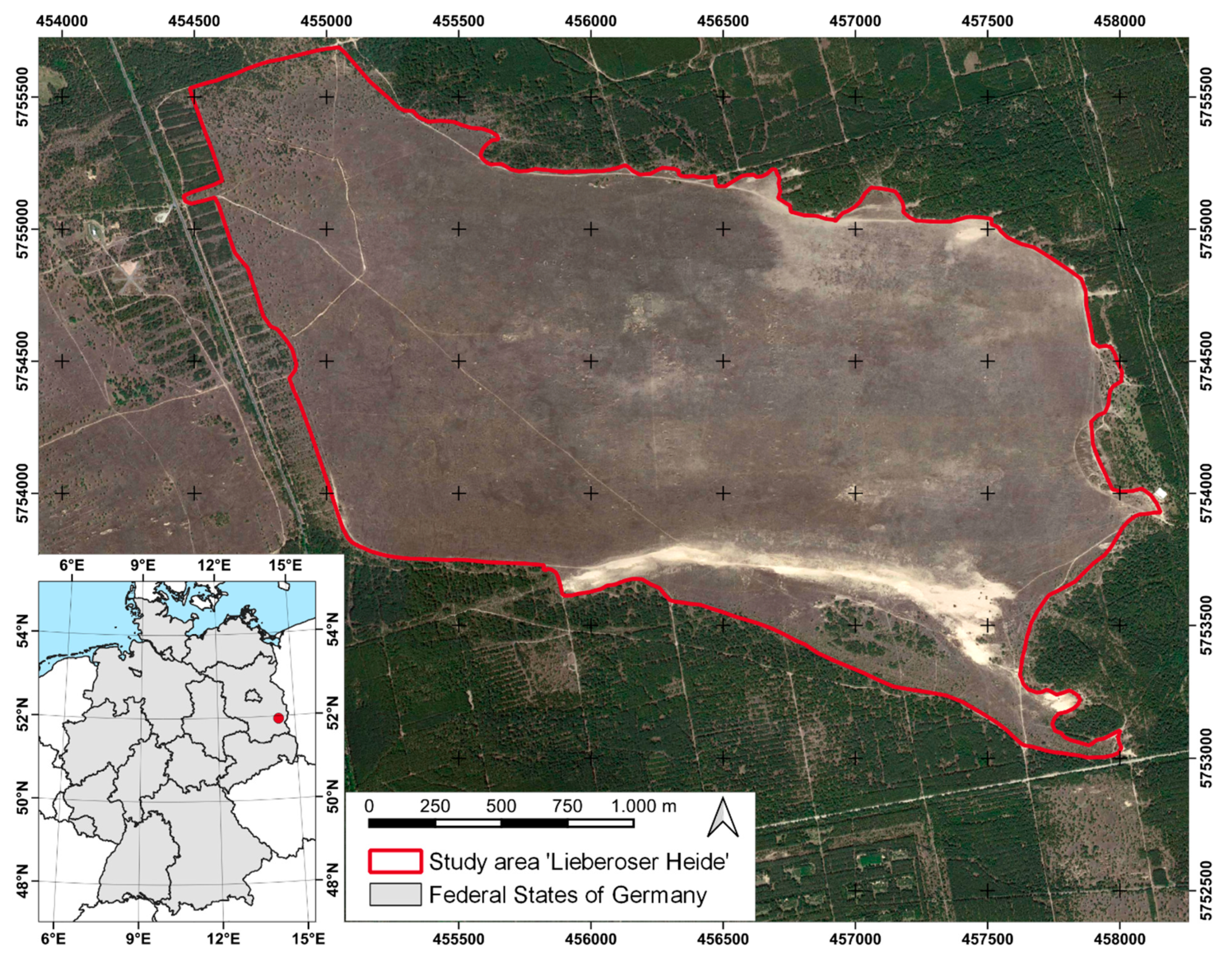
2.1. Study Area

Our study area (51°56′18″ N, 14°21′54″ E) is an open landscape located approximately 90 km southeast of the German capital Berlin and about 20 km north of the city of Cottbus in the Federal State of Brandenburg (Figure 1). It covers an area of 530 ha, commonly known to locals as ‘Lieberoser Heide’ referring to a generally flat (altitudes between 76 m and 90 m.a.s.l.) heath landscape. The region is characterized by the transitional Atlantic to continental climate. Long-term (1991–2020) average annual precipitation at the climate station Cottbus (ID 880; 51°46′33″ N, 14°19′3″ E, 69 m.a.s.l.) is 566 mm, with a clear peak during the summer season. The average annual temperature for the same period is 10.1 °C, whereby during the winter months, temperatures reach the point of freezing while the summer is warm.

Late Pleistocene influences shaped the region as it comprises parts of the southernmost German top moraine zones and features the complete glacial series, including large sand dune areas made up of gravel and sand. Sandy brown earth and podzol fine-grained soil with mainly silt and clay are prevailing [73]. The study site is completely unsettled. It is surrounded by forest with mainly Scots pine (Pinus sylvestris) stands and Silver birch (Betula pendula) trees to a lesser extent. The site was initially cleared by a forest fire in 1942 and subsequently used as central Europe’s largest military training area from 1945 to 1994 [74]. Later, the natural vegetation and soil were persistently disturbed and exposed to wind erosion, causing higher vegetation to settle very sparsely only [15]. Wind erosion caused the development of an initial mobile sand dune on the Pleistocene sand [17], which is the morphologically dominant feature in the otherwise flat area. Ever since the troops’ withdrawal in 1994, the study site has been under strict nature conservation, protecting it from human activities and ceded to natural succession. This led to the development of dry acidic grassland together with BSCs [17].

In the study area, the dry acidic grassland is dominated by Corynephorus canescens [12] (grey hair-grass) and heath vegetation dominated by Calluna vulgaris [16], and succession and spatial patterns of different BSC communities can be found. According to the various successional stages, these are: (i) initial green-algae BSCs (e.g., Zygogonium ericetorum and Klebsormidium flaccidum), (ii) moss-dominated BSCs (e.g., Polytrichum piliferum), and (iii) soil lichen (with mosses)-dominated biocrusts with various Cladonia species (e.g., Cladonia fimbriata and Cladonia coccifera) [15,75]. Different stages (e.g., photosynthetic activity, community respiration, and nitrogen fixation cycles) were characterized in various studies, e.g., [70,76]. Since the poikilohydric organisms, mosses, and lichens largely depend on the precipitation input, the changes in their hydration during dry–wet cycles influence their ecophysiological performance and structure, subsequently influencing the spectral reflectance [71,77].

2.2. Dataset Construction and Data Processing

Our analysis was built on a dataset constructed from in situ data, gridded time series of multispectral indices and bands derived from Sentinel-2 (S2) satellite images, and gridded topographic attributes (TAs) to parameterize the Random Forest (RF) classification approach for spatiotemporally estimating and mapping the BSC coverage in the study area (Figure 2). By incorporating daily precipitation data, the analysis of the seasonal and rainfall event-based BSC activity was driven.

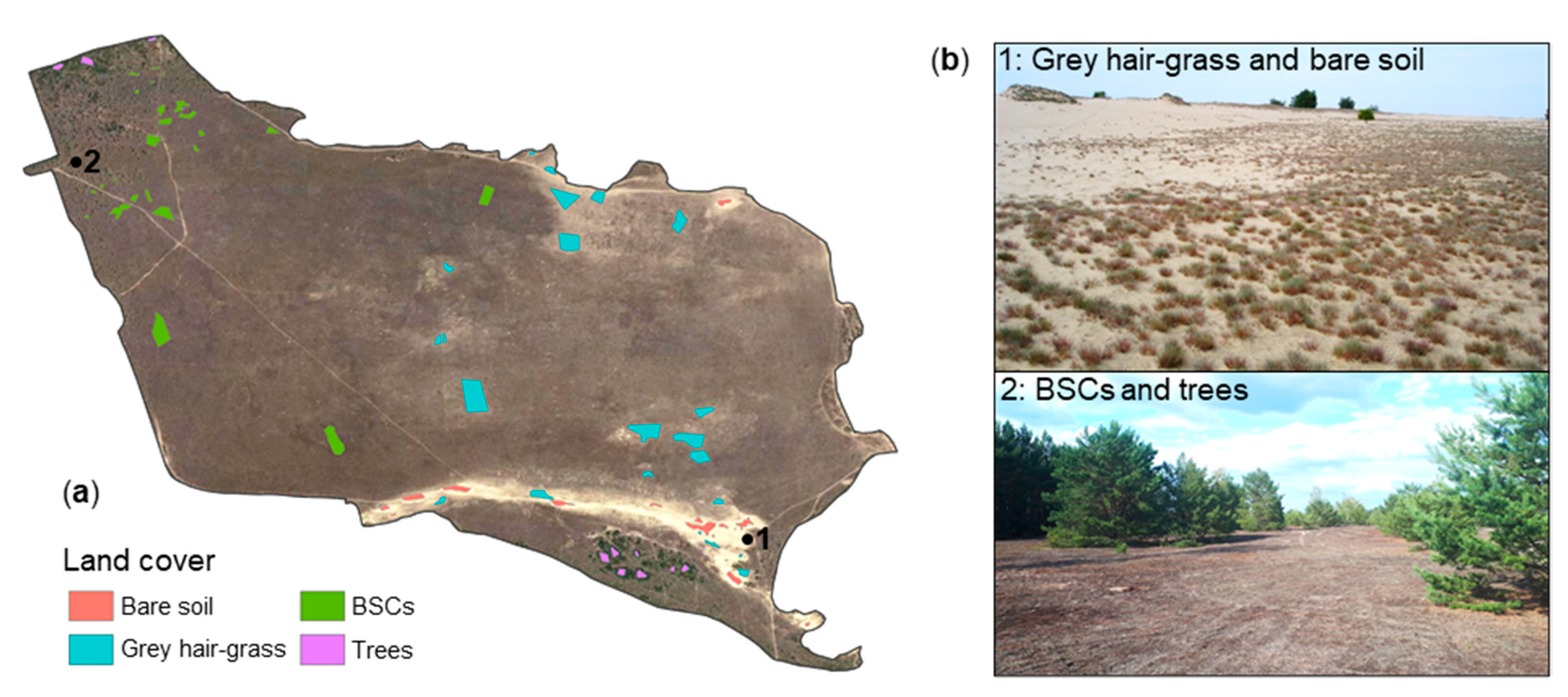
2.2.1. In Situ Data Collection

General reference data for training and testing the RF classification model are the most meaningful when collected in situ. However, due to its status as a natural conservation area and ammunition contamination resulting from the time when the study area was used as a military training site, access for in situ data collection was not entirely possible. Therefore, reference areas of the four dominant land cover classes (i) biological soil crust (BSCs), (ii) trees, (iii) grey hair-grass, and (iv) bare soil were sampled based on expert knowledge from previous field trips and Google Earth Pro high-resolution satellite imagery from 2018 and 2019 (Figure 3). This was considered as feasible as the land cover in the study site is assumed to not show variations during our observation period (2015–2020). Only polygons featuring one clearly distinguishable single land cover class homogenously were used as reference areas (Figure 3). Due to the 10 m spatial resolution of the S2 data, only reference polygons featuring one single land cover class within 20 m × 20 m areas and an additional 10 m buffer to areas of the other classes were sampled to avoid mixed S2 pixels. Using the R Project for Statistical Computing (version 4.1.0) [78], these polygons were converted to points (Figure 2) where each represented one S2 pixel. Thus, mixed pixels were reduced, and splitting of the reference data into more training and testing pixels via the k-folding approach (c.f., Section 2.3) was enabled.

2.2.2. Meteorological Data

We retrieved hourly recorded precipitation data from the Climate Data Center portal of the German Weather Service DWD (https://cdc.dwd.de/portal/, access on 8 February 2021). The DWD station Lieberose (ID 2997; 51°59′10″ N, 14°18′18″ E, 47 m.a.s.l.) is located closest to our study site with a distance of 4.8 km in the northwest direction. Therefore, we acquired data from this station and calculated cumulative daily precipitation (mm) to be incorporated in our further analysis.

In addition, information on the hourly wind direction 10 m above ground (in degrees) recorded at the DWD station Cottbus (ID 880) at a distance of 17.3 km from our study area was retrieved. It was used to detect the average wind direction between 1983 and 2020 (190°, corresponding to south), which was incorporated in the calculation of the TA ‘wind effect’ (c.f., Section 2.2.4).

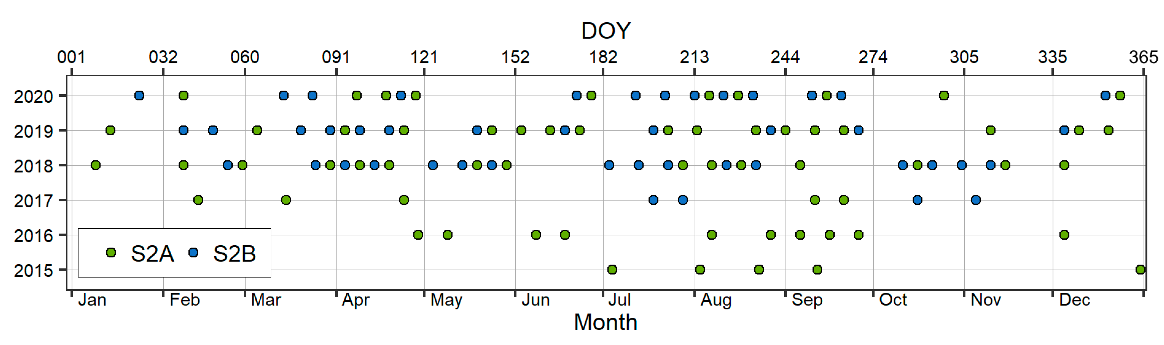
2.2.3. Sentinel-2 Data Preprocessing and Derivation of Multispectral Indices

We used Sentinel-2 (S2) data from the European Space Agency’s Copernicus mission for our analysis. With the twin constellation of the two polar-orbiting satellites S2A (launched in June 2015) and S2B (launched in March 2017) placed in the same sun-synchronous orbit, the temporal resolution of the system is five days. Both identical satellites carry an optical payload with visible (VIS), near-infrared (NIR), and shortwave infrared sensors (SWIR) [79]. The multispectral sensors operate with 13 spectral bands with a geometric resolution ranging between 10 m (four bands), 20 m (six bands), and 60 m (three bands). The swath width of S2 is 290 km. Data were retrieved from the ESA Copernicus Open Access Hub (https://scihub.copernicus.eu, accessed on 4 March 2021) and from the CREODIAS Repository platform (https://finder.creodias.eu, accessed on 4 March 2021).

S2A and S2B jointly captured a total of 358 images covering our study area, spanning the period from 4 June 2015 (S2A) to 29 December 2020. The S2 products were retrieved from descending sensing nodes as Level-1C (L1C) top-of-atmosphere (TOA) ortho-images, distributed in 100 × 100 km² tiles in WGS84 projection [80]. Our study area is located at the center of the tile 33 UVT. The L1C products were converted to Level-2A (L2A) products featuring bottom-of-atmosphere (BOA) reflectance corrected from atmospheric effects and terrain distortions by using the Sen2Cor preprocessor, implemented in the Sen2r R package [81]. Afterwards, the L2A tiles were cropped to the extent of the study area and reprojected to WGS84 UTM zone 33N (epsg code 32633). The further preprocessing aimed at cloud removal and cloud masking to minimize noise and enable a derivation of robust multispectral indices. We applied the Function of Mask (FMask, version 4.2) algorithm [82] to the L1C data, as it was proven to provide the most accurate results for S2 data [83]. It returned a classification for each scene, where areas covered by clouds, cloud shadow, and snow are depicted. These were subsequently masked out to only proceed with genuine land surface information under clear-sky conditions.

From a total of 358 S2 acquisitions, 220 (61%) images exhibited full cloud coverage, including shadows. From the remaining 138 scenes, 49 (13%) of the images were acquired under full clear-sky and snow-free conditions. By applying a threshold of 20% valid surface information within the study area, 107 S2A/B L2A products, spanning the years from 2015 to 2020 (Figure 4), were identified as appropriate for our analysis. Eventually, the number of “analysis-ready” scenes for our analysis were as follows: 5 scenes in 2015, 10 scenes in 2016, 9 scenes in 2017, 31 scenes in 2018, 29 scenes in 2019, and 23 scenes in 2020 (Figure 4).

While preprocessing the S2 scenes, we detected an offset between the data recorded by S2A and S2B. While S2A itself is very precise, S2B data deviates to S2A as well as among itself. The deviation between the two sensors could be quantified to up to 10 m, equivalent to one pixel, mainly in the north and east directions. This, of course, introduces inaccuracies when making pixel-based comparisons. However, as the majority of the scenes are congruent and we constantly incorporated a wide range of pixels, we chose to proceed without co-registering the images. As this is only doable for satellite scenes with low cloud coverage, this would not have been applicable to all images. Of course, we have to keep this in mind for the upcoming analysis.

Only the four bands available at the highest resolution of 10 m (i.e., blue, green, red, and NIR) were used in this study, as they sufficed for generating all relevant indices. We computed the following four different multispectral indices that were reported to be meaningful for RS-based analysis of BSCs for each individual scene using Equations (1)–(4): NDVI [49], CI [26], mCI [28], and BSCI [27]:

NDVI = (R_NIR − R_red)/(R_NIR + R_red),

(1)

CI = 1 − (R_red − R_blue)/(R_red + R_blue),

(2)

mCI = 1 − (R_green − R_red)/(R_green + R_red)

(3)

BSCI = (1 − L × |R_red − R_green|)/R^mean_greenredNIR

(4)

where R_blue, R_green, R_red, and R_NIR are the surface reflectance ranging from 0 to 1 at the blue, green, red, and NIR bands, respectively, corresponding to S2 band numbers 2, 3, 4, and 8. L is an adjustment parameter to amplify the absolute difference between R_green and R_red. It was set to the value of 2, and R^mean_greenredNIR is the mean reflectance of the green, red, and NIR bands [27].

2.2.4. Topographic Attributes

Topographic attributes (TAs) are commonly applied to quantitatively describe landform characteristics and structures [84] and as proxy-drivers in environmental modeling, e.g., [85], and are readily available as computed derivates from Digital Elevation Models (DEMs) [86]. In Brandenburg, the Federal State’s Department of State Survey and Geospatial Base Information provides DEMs in a high spatial resolution of 1 m (post-processed airborne LiDAR data acquired on 19 March 2010) free of charge through its web application (https://geobroker.geobasis-bb.de, access on 13 June 2020). A mosaic of six DEM tiles (each with 1 × 1 km²) was converted to GeoTiff and cropped to a bounding box capturing the study area. From this, a total of 13 TAs (

Table 2. Topographic attributes calculated in SAGA GIS and their relevance as predictors used in the Random Forest classification model for mapping the biological soil crusts in the study area.

Attribute (unit)	Relevance
Aspect (degree)	the landscape’s spatial heterogeneity affecting the surface energy balance and through this, the soil water retention capacity and water availability [88]
Elevation (m.a.s.l.)	the physical landscape properties and their spatial patterns, and key attributes for the further derivation of terrain-shape indices
Flow accumulation (-)	the effects of the depth and velocity of flow (here by integrating the multiple flow direction based on the maximum downslope gradient; top-down processing) [89]
Insolation (W m−2)	the annual sum of direct and diffuse potential incoming solar radiation calculated according to times of sunrise and sunset [90]
Topographic openness (positive and negative; rad m−1)	the dominance (positive) or enclosure (negative) of a landscape location [91]
Plan curvature (rad m−1)	the contour line formed by intersecting a horizontal plane with the surface, thus a proxy on the convergence or divergence of water during downslope flow [88]
Profile curvature (rad m−1)	the surface in the direction of the steepest slope, thus a proxy on the acceleration/deceleration of surface water [88]
Slope angle (degree)	the landscape’s spatial heterogeneity and catchment-related hydrological processes (e.g., flow direction, water runoff velocity and accumulation) [88]
Topographic Position Index (TPI; -)	the topographic slope positions and for landform classifications [92]
Terrain Ruggedness Index (TRI; -)	the surface heterogeneity of the landscape; averaged from the absolute differences in elevation between a focal cell and its eight neighboring DEM cells [93]
Topographic Wetness Index (TWI; -)	the topography’s spatial scale effect on hydrological processes and proxy on the terrain-related soil moisture potential [94]
Wind Exposition Index (WEI1; -)	the wind shadowed pixels/areas (values < 1) and pixels/area that are exposed to wind (values > 1) [95]
Wind Effect Index (WEI2; -)	The direction in which the wind is going (windward/leeward index) [95]

) were calculated representing continuous primary local TAs (i.e., elevation, aspect, slope angle, plan, and profile curvature) and secondary compound TAs (i.e., flow accumulation, topographic position, ruggedness, wetness index, and wind exposition and effect). Their DEM-based computation was performed using SAGA GIS (version 2.3.2) [87]. To meet the same pixel size of the S2 input data, we resampled the gridded TAs to a joint geometric resolution of 10 m to be incorporated into our modeling framework supporting the classification (Figure 2).

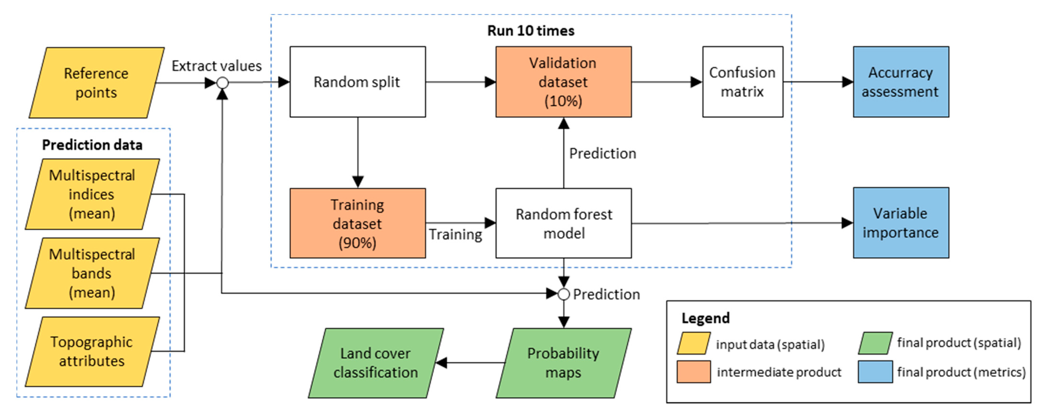
2.3. Biocrust Mapping and Response to Rainfall

2.3.1. Estimating Biological Soil Crust Coverage

We applied an RF classification analysis [67] using the R-package randomForest version 4.6-14 [96] to estimate the spatial distribution of the BSC cover by classifying the study area into the four dominating land cover classes (c.f., Section 2.2.1). RF is an ensemble ML method for classification and regression, combining numerous tree predictors voting for the most popular class, growing by selecting random features in the training dataset [67]. It also works well using high-dimensional input variables [97].

The model requires two input parameters: reference areas and predictors (Figure 2). Our sampled reference areas (c.f., Section 2.2.1) included 1,085 S2 pixels partitioned into 322 (29.7%) for the class ‘biological soil crusts’ (BSCs), 73 (6.7%) for the class ‘trees’, 564 (52%) for the class ‘grey hair-grass’, and 126 (11.6%) for the class ‘bare soil’ while the entire study area is captured by 53,139 S2 pixels. The predictors are the parameters the classification was performed on. In our study, these were the multispectral data (i.e., the calculated indices and the individual bands in 10 m spatial resolution; c.f., Section 2.2.3) and the TAs (Table 2). As we aimed at one classification valid for the full timeframe, all multispectral parameters were integrated over the whole observation period (2015–2020) using all 107 analysis-ready acquisitions (c.f., Section 2.2.3) via the pixel-based mean. This was considered feasible, as the land cover in the study site is not subject to short-term variations. The RF algorithm resulted in one probability map for each class (c.f., Section 3.2), containing each pixel’s probability of matching the respective class. In the discrete classification map (c.f., Section 3.3.1), pixels were strictly assigned to the class with the highest probability.

Model training and testing and the accuracy assessment were performed using k-fold cross-validation [98], a commonly used method where the reference data is randomly split into k (in this study ten) disjunct subsets. The model was then run ten times, each time using nine of the subsets for training and one of the subsets for testing (Figure 2). The results of each run were assessed and averaged across all ten replicates. This approach was superior to simply splitting the data into strictly one portion for training and one for testing, as this could lead to overfitting and biased accuracy estimations.

Our RF-based approach also provided measurements for evaluating the importance of the predictors to the performance of the model: (i) the mean decrease in accuracy (MDA), measuring how much accuracy is lost in percent when the respective variable was permuted from the model and (ii) the mean decrease in Gini coefficient (MDG), measuring how much each variable contributes to the homogeneity of the nodes in the resulting RF model [99].

To obtain information on the classification results corresponding to reality, we conducted an accuracy assessment [100] by applying the trained model on the test data, i.e., the portions derived from the reference dataset by the k-folding approach. Therefore, a confusion matrix was used to compare the classified pixels with the test data for each fold and then averaged. Four measures of accuracy were calculated for each class based on this matrix [100]: (i) overall accuracy (OA), revealing the overall model performance, (ii) user’s accuracy (UA), providing information on how well the classification results match the classes in reality, and (iii) producer’s accuracy (PA), indicating the proportion of correctly classified pixels. The kappa coefficient of agreement (K^) returns the extent to which the result differs from a random classification.

2.3.2. Analyzing the Seasonal and Rainfall Event-Based Activity of Biological Soil Crusts

The areas classified as BSCs were subsequently used to retrieve information on dry and wet cycles. We used the NDVI for assessing the change in metabolic activity of BSCs, i.e., under wet conditions after precipitation events and under dry conditions, when the activities are reported to be suspended (c.f., Section 1). We compared the S2-based NDVI data from the available 107 acquisitions (c.f., Section 2.2.3) to daily precipitation data measured at the weather station Lieberose (c.f., Section 2.2.2). Hereby, we evaluated whether the postulated effect can be depicted in our study area using the characteristics of the S2 sensor in terms of spatiotemporal resolution. A one-way ANOVA was tested for explanatory rainfall response examples to investigate if the NDVI values for the class ‘biological soil crust’ (BSC) differ significantly under dry and wet conditions. Additionally, the response behavior was evaluated using change detection between NDVI grids representing dry and wet conditions, respectively, to visualize spatial patterns of change in BSC’s activity.

Moreover, we investigated seasonal trends of BSCs. To increase the temporal density of our time series and obtain meaningful information on the average seasonal trend, we merged all NDVI grids from five years into one. This was especially important for the earlier years, where only one sensor (i.e., S2A) was operating, causing a low temporal resolution (Figure 4). A polynomial trend line was calculated to illustrate the temporal course of activity through one average year. The range of NDVI values was compared for each season, tested for significant differences using one-way ANOVA. The seasons are hereby defined as winter (December–February), spring (March–May), summer (June–August), and autumn (September–November).

3. Results

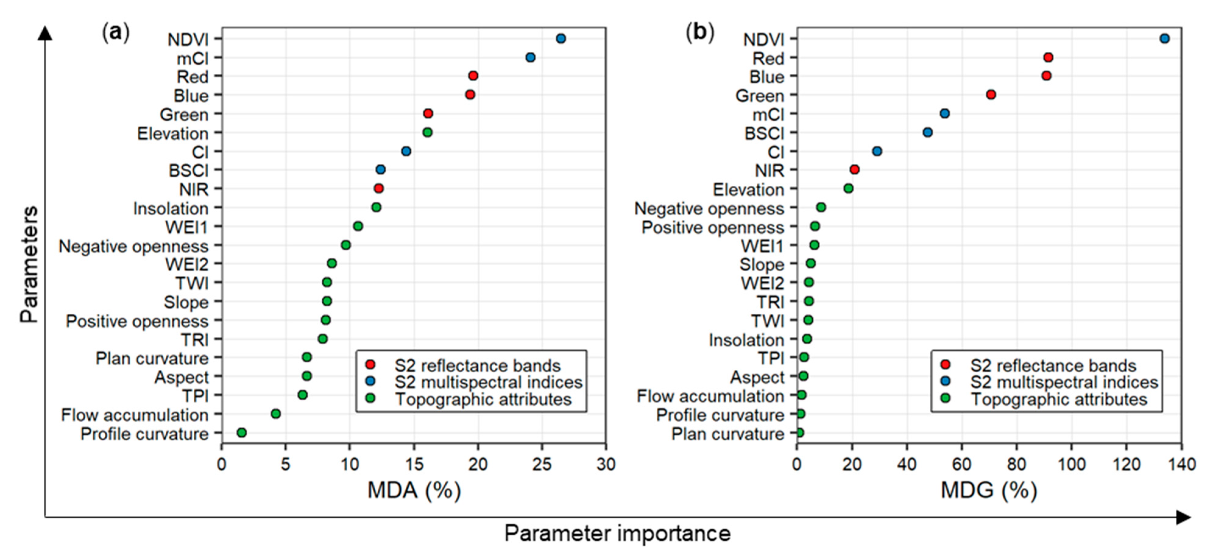
3.1. Performance of the Random Forest Classification Model

The accuracy assessment returned an OA of 98.9% and a Κ^ of 0.9822 when validated against the 10-fold based test dataset. The UA is 96% for the class bare soil, 98.6% for trees, 99.1% for grey hair-grass, and 99.6% for BSCs. The values of PA are 96% for bare soil, 98.9% for grey hair-grass, 99.6% for BSCs, and 100% for trees. The higher the classes’ accuracies, the more the algorithm is capable of distinguishing them, resulting in less misclassification. The classification can therefore be categorized as highly accurate.

This also provides legitimacy concerning the predictor importance information (Figure 5). Hereby, the predictors are ranked according to their importance in estimating and differentiating the land cover classes as determined by the RF classification model. Higher values refer to a higher importance of the corresponding parameter within the classification.

In general, the S2-based multispectral predictors, i.e., the spectral bands and indices, were detected as more important than the TAs employed. Hereby, the NDVI is by far the most crucial variable (Figure 5). Concerning the spectral bands, those sensing in the visible spectra (i.e., red, green, and blue) were identified as more important than the NIR band (Figure 5). With regard to the multispectral indices, the mCI ranks second, followed by the CI and the BSCI. Among the TAs, elevation was identified as the most important parameter (Figure 5), revealing approximately the same parameter importance as the green spectral band and the NIR (Figure 5). Descending importance was revealed for the TAs representing the exposition to and the effect of wind (WEI₁ and WEI₂), the insolation, and the topographic openness in the study area. Flow accumulation, TPI, and curvature contributed the least to the classification (Figure 5).

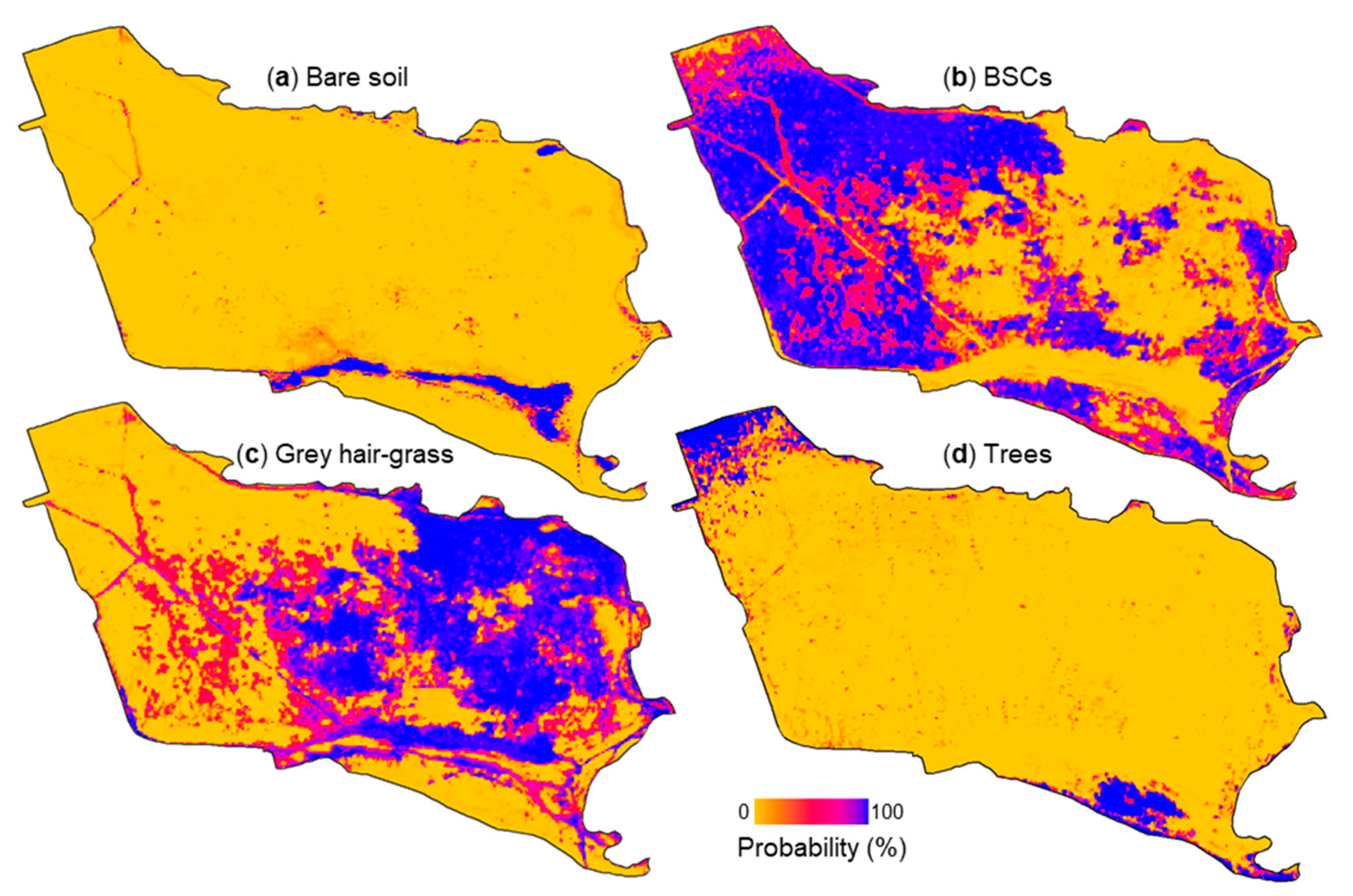
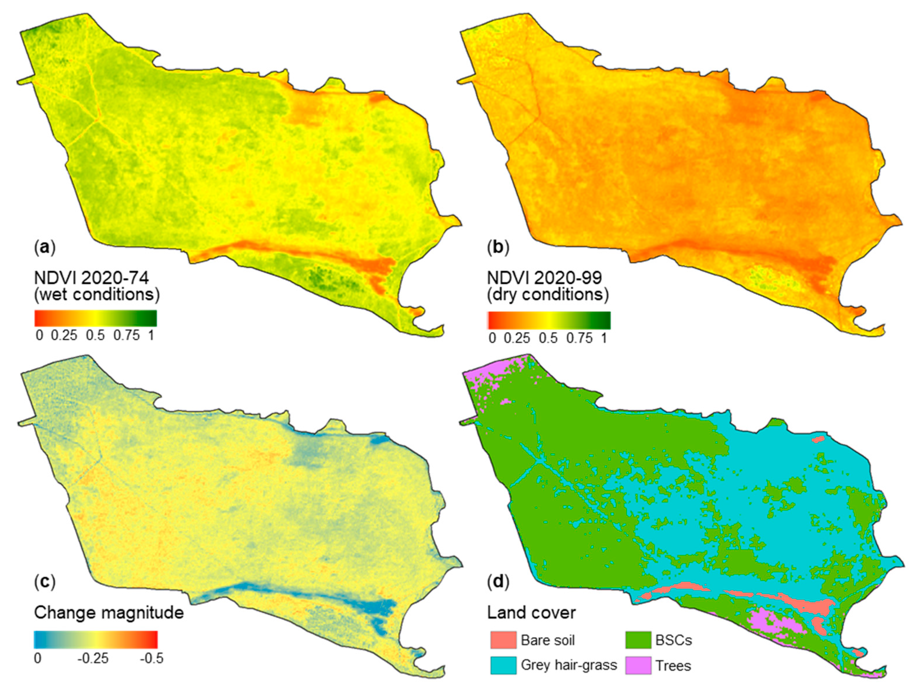
3.2. Estimated Biological Soil Crust Coverage

As revealed in the RF-based classification, our study area (531.4 ha in total) classifies into 10.07 ha (1.9%) of bare soil, 287.3 ha (54.1%) of BSCs, 219.25 ha (41.3%) of grey hair-grass, and 14.77 ha (2.8%) of trees (Figure 6 and Figure 8d). Hence, BSCs were identified as predominating land cover within the ‘Lieberoser Heide’. Tree cover is mainly present in the northwest of the study area and south of the sand dune (Figure 6). The sand dune was classified as the most extensive bare soil feature. With a small transitional zone to the bare soil, grey hair-grass was classified, creating a buffer surrounding the dune. Grey hair-grass also dominates the central and eastern study area (Figure 6c), where biocrust-dominated patches gradually blend in (Figure 6c), creating large transitions. BSCs were classified as expansively and continuously present in the western and northern study area (Figure 6b). In the very northwest, they mix with the class ‘trees’.

In the final classification map (Figure 8d), pixels were strictly assigned towards their dominant land cover class. This implies the presence of minor patches of other land cover types, and the assigned one has the highest share and therefore dominates the spectral signature. In the case of the study area, this is especially true regarding the intersection of the classes ‘biological soil crust’ (BSC) and ‘grey hair-grass’, and the fluctuating density of grey hair-grass on the sandy bare soil areas. Therefore, information on the transitional zones of the classes can be derived from the probability maps showing the probability for each pixel to be assigned to an individual class (Figure 6a–d).

3.3. Dry and Wet Cycles of Biological Soil Crusts

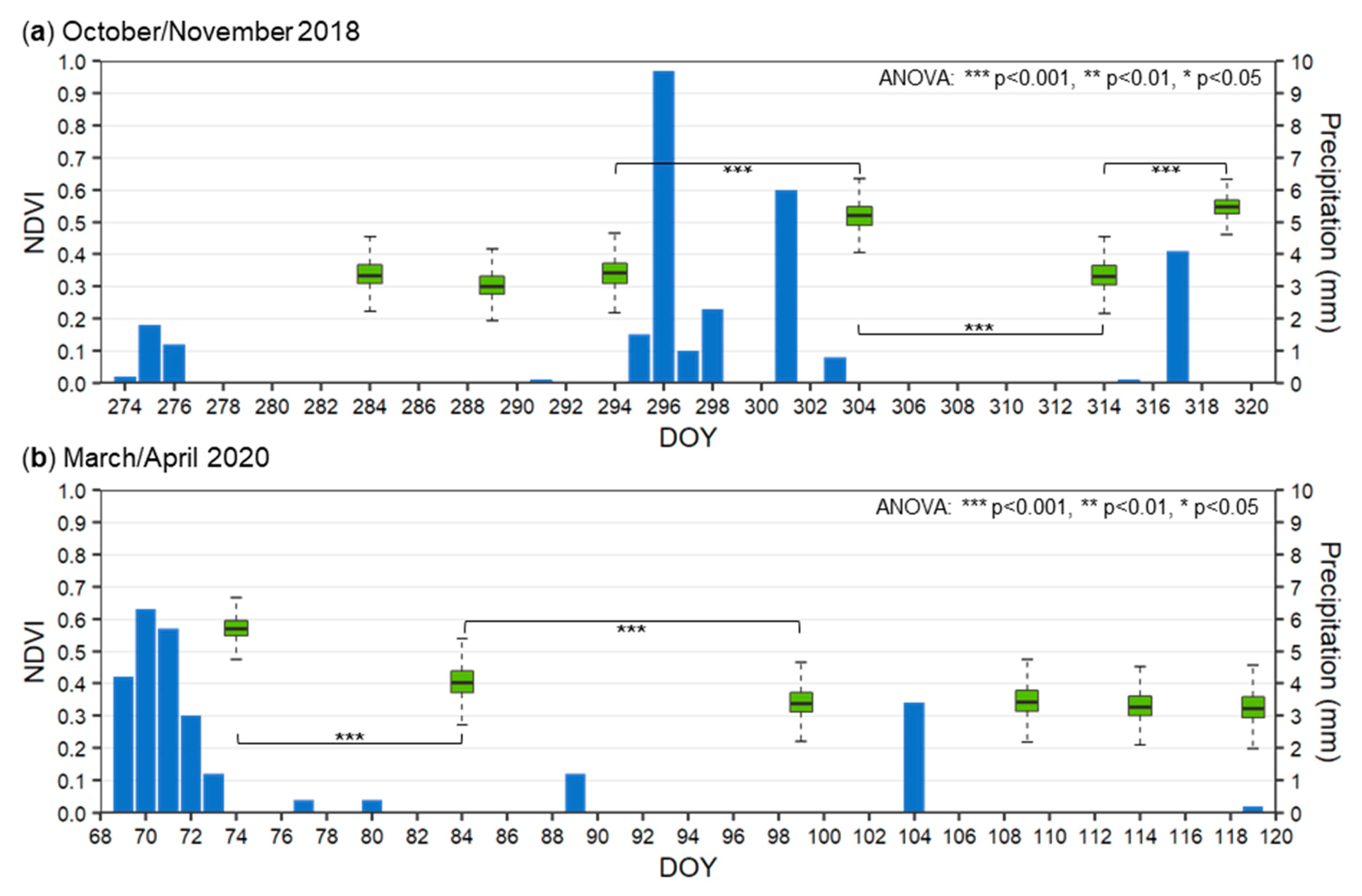
3.3.1. Activity of Biological Soil Crusts in Response to Rainfall Events

In order to obtain information on the direct response of the areas classified as BSCs to rainfall, at least two cloud-free scenes close to rainfall events were required, i.e., to capture the BSC’s metabolic activity represented by the NDVI before and after rainfall. However, only 107 adequate S2 scenes over the period of 2000 days led to an average temporal resolution of around 18.7 days (Figure 4), making the time series relatively coarse, thus likely constrained to accurately map short-term changes. Due to these inconsistencies, a meaningful analysis over the whole observation period was not feasible. Therefore, explanatory periods where the temporal resolution was assumed sufficient to depict rainfall-induced changes were selected. We focused on the two most significant ones, located in October/November 2018 and March/April 2020 (Figure 7).

The first example period shows a longer dry period between DOY 277 and DOY 294, whereby the NDVI of the BSC areas exhibit median values of 0.3 to 0.35 (Figure 7a). Within the nine consecutive days, 21.3 mm of rain was recorded at the climate station in Lieberose (c.f., Section 2.2.2), after which the median NDVI increased significantly up to 0.52 (Figure 7a). During the following eleven dry days (DOY 304 to 314 with a cumulative rainfall of 0 mm), the NDVI decreased to its initial level at DOY 294 (Figure 7a). A similar behavior of NDVI (i.e., increase in NDVI after a rainfall event) can be observed between DOYs 314 and 319 (Figure 7a). Therefore, two levels of NDVI values can be observed: NDVI values around 0.55 for wet and NDVI values around 0.33 for dry conditions (

Table 3. Descriptive statistics of the Sentinel-2-based NDVI observations for the two example periods from day-of-year (DOY) 273 to 321 in October/November 2018 and from DOY 68 to 120 in March/April 2020 for each land cover class separated for dry and wet conditions. Hereby, the NDVI values for DOY 84 in 2020 were omitted, as they represent intermediate conditions.

Statistics	Total	Biological Soil Crusts		Bare Soil		Grey Hair-Grass		Trees
		Dry	Wet	Dry	Wet	Dry	Wet	Dry	Wet
Nr. of observations (i.e., pixels)	535,875	208,967	86,190	6860	3021	149,595	65,775	11,036	4431
Minimum	0.073	0.138	0.248	0.073	0.078	0.090	0.099	0.278	0.402
1st quartile	0.273	0.301	0.520	0.108	0.124	0.231	0.392	0.464	0.636
Median	0.329	0.329	0.548	0.123	0.159	0.255	0.451	0.514	0.681
3rd quartile	0.450	0.364	0.575	0.141	0.199	0.275	0.494	0.575	0.736
Maximum	0.894	0.645	0.759	0.439	0.517	0.544	0.680	0.805	0.894
Average	0.361	0.335	0.546	0.126	0.168	0.251	0.438	0.522	0.686
Standard deviation (SD)	0.121	0.047	0.045	0.026	0.054	0.037	0.076	0.077	0.070
Coefficient of variation (%)	33.2	14.1	8.3	20.8	32.2	14.6	17.3	14.8	10.2

).

The second example period (Figure 7b) confirms this observation, as the two different NDVI levels can be seen at DOY 74 and from 99 to 120, respectively. Additionally, DOY 84 shows an intermediate value of decreasing NDVI, indicating the process of gradual drying. Interestingly, the precipitation event of 3.4 mm at DOY 104 did not affect the NDVI values recorded five days later, which are at the same level as before the rainfall (Figure 7b).

Table 3 depicts the descriptive statistics of the NDVI values for dry and wet conditions over all land cover classes within the example periods (Figure 7). It can be observed that bare soil values are the least subject to change from dry to wet conditions, with the median changing by approximately 0.04 (Table 3). The median changes from dry to wet for grey hair-grass amount to approximately 0.17, and to approximately 0.18 for trees and 0.22 for BSCs, respectively (Table 3). Thus, BSCs are observed to exhibit the highest changes in median NDVI between dry and wet conditions.

The rainfall response was also analyzed on a spatial basis. Figure 8 shows the associated NDVI grids for the observations at DOY 74 and 99 in 2020 for the entire study area, including all land cover classes. Here, DOY 74 refers to wet conditions, whereas the observation at DOY 99 represents dry conditions, i.e., after 10 days without rainfall (Figure 7). Additionally, the change between the two NDVI observations is depicted indicating that areas in the western and northern (Figure 8c) areas are subject to the highest changes in NDVI.

3.3.2. Seasonal Trends in the Activity of Biological Soil Crusts

The number of observations (i.e., S2 scenes) during spring and summer is much higher than during autumn and winter (c.f., Section 2.2.3). However, when merging all available 107 NDVI scenes capturing the entire observation period into one single aggregated year, a significant trend and seasonal differences showing a distinct phenological (i.e., referring to the metabolic activity) pattern can be observed (Figure 9). The NDVI values are significantly higher during the winter season (median 0.49, SD 0.08) when compared to the spring (median 0.34, SD 0.06) and summer (median 0.3, SD 0.03) seasons (Figure 9b). In autumn, the NDVI increases again significantly (median 0.36, SD 0.08) (Figure 9b). When comparing the autumn to the spring season, no significant differences in NDVI can be observed (Figure 9).

4. Discussion

4.1. Land Cover Classification and Biological Soil Crust Coverage Estimation

The very high overall RF-based classification accuracy (98.9%) indicates that our applied classification approach is meaningful. It corresponds well to the reality, and hence is considered successful in delineating BSCs in our study area. Particularly, the class ‘trees’ exhibited very high producer’s accuracy (c.f., Section 3.1) as they represent distinct features when compared to BSCs, bare soil, and grey hair-grasses, thus are clearly distinguishable from all other. There is only a tiny portion of tree pixels wrongly assigned to the BSC class, originating from the northwestern study area. Here, they are presently isolated within and on top of BSCs. Bare soil exhibits the lowest accuracy—which is still very high—as it tends to be confused with grey hair-grass. This originates from sampling the latter primarily in areas where bare soil is the background substrate, like in the immediate surroundings of the sandy top of the dune. Grey hair-grass is never present alone, as it grows in clusters on top of mainly sand and BSCs. When it mixes with BSCs, it is not distinguishable as the small isolated tufts do not highly contribute to the spectral signature on these scales. This is also why grey hair-grass shows the most spectral similarities with the bare soil values for all of the indices. It is surprising that BSCs and grey hair-grass do not get confused more often, as they resemble themselves concerning CI and mCI indices and show large transitional zones in the area of interest. Additionally, regarding the NDVI, they reveal similar values. The BSCI, however, is able to differentiate them quite well.

When classifying the different land cover types, the multispectral predictors reveal higher importance than the TAs (Figure 5). Hereby, the NDVI is by far the most crucial predictor. This is not very surprising, as it is a known meaningful index concerning plant physiognomy and activity, and coincides with previous observations, where the index band combination NIR and red was found to be the most crucial predictor in estimating BSC cover [28]. The mCI was identified as the second most important index, as it is able to differentiate BSCs from other types of higher plants [28]. Additionally, the CI, targeting cyanobacteria [26], and the BSCI, developed especially for lichen-dominated biocrusts [27], performed well (Figure 5). Concerning the individual spectral bands, red, blue, and green show importance comparable to the indices, with only NIR being a little less important (Figure 5). This confirms that adding the raw bands and not only relying on indices is able to increase the classification accuracy.

For our study, we cannot conclude that the distribution of the different land cover classes is highly influenced by the topography, as the TAs were identified as not distinctly important in the classification. However, from all TAs, elevation reveals the highest importance (Figure 5). This originates from the dune on the one hand, as most of the bare soil is located on the ridge. On the other hand, the fact that grey hair-grass is mainly located in the lower central-eastern area at elevations from 75 to 80 m.a.s.l., and biocrust coverage is highest in the northwestern plateau, located at higher elevations from 85 to 90 m.a.s.l., certainly also influences the importance. There might also be some bias in the training data, as the distribution of the biocrust samples is concentrated on this plateau. However, this was inevitable, as this area is the only one where the BSC cover was known to be high from previous investigations. Similar to the elevation, the relatively high-ranked wind attributes WEI₁ and WEI₂ (Table 2) are influenced by these effects, as the highest wind effects are also detected for the plateau and the dune, which the bare soil class is mainly located on top of. This confirms that the wind attributes represent reality quite well, as, without the wind effect, no bare sand areas would exist at the dune.

It is arguable whether including the TAs into the classification is beneficial, as the parameter importance implies otherwise (Figure 5). Therefore, we ran the RF model a second time using multispectral parameters only, and the resulting classification did not show high differences in terms of accuracy. Thus, we conclude that including TAs of 10 m spatial resolution into the RF-based classification was not highly beneficial in our study site, as the prevalent very small-scale topographic changes are severely smoothed when resampling from 1 to 10 m and therefore cannot be recognized anymore. The probability for each class was tested for correlation to the topography using the Pearson correlation coefficient. While other classes showed high correlations, BSCs only show small correlations to a few TAs, with 0.27, 0.16, and −0.12 being the highest numbers for Slope, WEI1, and Elevation, respectively. This confirms the statement that the biocrust coverage is not highly dependent on topography on a 10 m scale.

The land cover classes of the derived classification have to be interpreted as areas where the respective class is dominant in the spectral signature, as they are not strictly separable in reality and show transitional zones. This also implies that pixels assigned to one class may feature shares of other classes influencing the signal, which has to be considered when interpreting the rainfall response of classes. The approach of differentiating the four selected land cover classes is ideal for obtaining an uncomplicated and fast delineation of the BSC-covered areas. Using the temporal average for the multispectral predictors performed well, as confirmed by the high classification accuracy. Comparing the results to reality showed a plausible coincidence to expectations and could be evaluated on-site in a short field visit in the outermost northwest study area in Sep. 2020. We would like to reiterate that access to the study area is generally prohibited due to its natural conservation status (c.f., Section 2.2.1). We could observe that even though grey hair-grass is present in areas of high BSC probability, their percentage share can be neglected with regard to its spectral signature at a spatial resolution of 10 m, as the fascicles are considered as not distinctly contributing to the spectral signature.

4.2. Dry and Wet Cycles of Biological Soil Crusts

While the precipitation data is continuously measured at the climate station, the S2 NDVI time series is limited by two factors: the revisiting time of Sentinel 2 and the quality of the available scenes. Revisiting time is five days since the launch of S2B in March 2017. Before that, images are available only every ten days, severely limiting temporal resolution for the first two operational years. The highest drawback originates from clouds and snow, as affected areas cannot be used for the analysis. With the high probability of clouds, the most considerable portion (251/358, 70%) of satellite acquisitions is not appropriate for analysis (c.f. Section 2.2.3). This is one of the main factors that distinguishes areas in temperate climates from the semi-arid and arid drylands, as these show a much lower probability for cloud cover, making optical imagery available on a much more consistent basis. With the remaining 107 NDVI observations, the theoretical temporal resolution drops to 18.7 days, making it hard to connect them to precipitation events, as BSCs react quickly to them by recommencing their metabolic activities within a few hours. Often the observations cannot be easily assigned to dry or wet periods, as precipitation and drying events of different magnitudes alternate between them. Additionally, during summer the high temperatures and solar irradiation lead to higher evaporation rates, making the BSCs dry out much faster than during the other seasons and leading to no S2 observation able to detect the activity changes. Therefore, spring and autumn are the best periods to identify the rainfall response for our study area.

4.2.1. Activity of the Biological Soil Crusts in Response to Rainfall Events

The two selected explanatory periods of the time series show that the NDVI differs significantly (p < 0.001) for biocrusts under wet and dry conditions, and the change can be affiliated to precipitation events. When wet, BSCs tend to match the spectral characteristics and NDVI of higher green vegetation, such as fully grown crop fields [45], as the median reaches values of 0.55 (Table 3). After dry periods, the median NDVI drops down to 0.33, getting closer to bare soil values, which are below 0.16. These values and the magnitude of change (0.22) match observations from areas with high biocrust coverage within drylands [39].

We can also confirm the observation of studies performed in the Negev [2,37] that activity of BSCs persists for up to five days after precipitation events when the conditions are right. For example, the image for DOY 84 in 2020 was acquired five days after a small precipitation event of only 0.4 mm. The NDVI is still significantly higher than on DOY 99 after ten dry days, but also significantly lower than on DOY 74 after multiple days of larger rainfall events. This means that even such small precipitation events can influence the activity of BSCs over a period of five days, at least in spring, when the evaporation rates are low due to moderate solar irradiation and temperatures. It is arguable that the two minimal rainfall events of 0.4 mm each might just have prolonged the photosynthetically active time from DOY 69 to 73, where the biocrusts go into a “hold position” after large precipitation events and can be recommenced by small rainfall events [2,37]. In November 2018, in phenologically similar conditions, ten dry days were enough for the biocrusts to return to the same level of activity as before the rainfall event. The two observations of wet conditions were recorded one and two days after the precipitation event in this example, which means that during this phase, the activity has not declined.

The initiation phase of biocrusts after rainfall events, where the activity increases, could not be evaluated due to the lack of NDVI scenes immediately after precipitation events. We, however, could register that one day is enough for an activity resumption (c.f., Section 3.3.1). Here, the inconsistencies of the S2 NDVI time series are once again the limiting factor, as the most interesting parts are on the days directly before and after precipitation events. However, these days are more likely to be cloud covered, reducing the chance of obtaining an appropriate observation. In this study, there are hardly any images found to be acquired on the day of a large precipitation event or the next day.

The effect of rainfall events on the NDVI is not consistently clearly visible even though an observation might be available. The observation from DOY 2020–109, for example, is located just five days after a larger rainfall event amounting to 3.4 mm. While we already showed that five days are enough to detect activity even after small rainfall events, this is not the case for this observation, as the NDVI stays at the same level. It is unclear whether here the activity has already declined again due to a change in temperature and higher evaporation, or whether the rainfall was only recorded by the station but did not occur in the study area. Rainfall can exhibit high local variability on a small spatial scale, and we would like to stress that the climate station Lieberose (c.f., Section 2.1) is located at a distance of 4.8 km northwest and at a distance of 8.8 km southeast of our study area. This is assumed to not be close enough to ensure that each event occurring within the study site was detected by the station. The best example confirming this is the 18 mm of rainfall measured on 9 September 2019 (DOY 252), which only led to a very minor change in NDVI values of 0.05 (median) detected for the class ‘biological soil crusts’ two days later.

The median NDVI values of bare soil are constantly below 0.16 (Table 3), even under wet conditions, confirming that our classification performed well in delineating this class. Trees show the highest NDVI values as expected, but also a very high value range. This is most certainly because the trees within the study area are isolated and therefore the pixels may be influenced by signals from the surrounding land cover. The values of grey hair-grass are always lower than the ones of BSCs under both dry and wet conditions, with this difference being more pronounced after rainfall. While bare soil medians stay stable under dry and wet conditions and only their value range gets a little higher, grey hair-grass and trees show the same dry/wet pattern as BSCs. This originates from the discrete classification featuring dominant land cover (c.f., Section 4.2). As BSCs can exist below both grey hair-grass and trees, they of course influence the NDVI values. The fact that the highest difference of NDVI between dry and wet conditions was detected for areas classified as BSCs confirms the validity of our classification (Table 3), as the rainfall response patterns of NDVI are known to differ for various degrees of sub-pixel biocrust cover and are more significant with higher coverage [39]. When we transfer this hypothesis to the NDVI change map (Figure 8c), the pixels with the highest magnitude of change are the ones with the highest sub-pixel biocrust coverage, which are the ones in the very northern and central-western areas. In the very northwest, where the biocrust cover is known to be very pure and high, however, the change magnitude is not that high, which is the result of the trees scattered within this area returning a mixed signal.

4.2.2. Seasonal Trends in the Activity of Biological Soil Crusts

Due to the higher cloud and snow cover probability during the autumn and winter seasons in temperate climates, data gaps (resulting from fewer satellite observations available for analysis) are more likely than during the spring and summer seasons (Figure 4). However, aggregating all multitemporal data into one single year made it possible to generate a significant average seasonal trend for BSCs (Figure 9). It reveals patterns of BSCs with significantly higher average NDVI values during the winter season when compared to the summer season. This seems unusual for any vegetation within the temperate climates, as vascular plants usually show higher activity during the warm summer months before dying off or hibernating during the cold winter. However, BSCs are considered poikilohydric, i.e., being only active when sufficient water is available [2]. As in temperate regions, incoming solar radiation, and therefore air and soil temperatures, are higher during the summer [101]; higher evaporation rates are supposed to lead to less water available for, and therefore less metabolic activity of, the BSCs (Figure 9). This proposes a higher probability to detect active BSCs during the winter; however, this cannot be proven, as no agreeing studies could be identified.

For the years 2018 and 2019, a higher amount of adequate (i.e., no to only a few clouds) RS-based observations were available due to the occurrence of extraordinary hot and dry summers, being ranked 2nd and 3rd warmest since 1881 by the DWD for all of Germany [102]. The effects in 2018 were even more pronounced in the northern and eastern parts of Germany, including our study area [103]. When analyzing the rainfall data from the Lieberose weather station (c.f., Section 2.2.2), the long-term (1991–2020) average annual precipitation was 557 mm, while in 2018 and 2019, only 398 and 467 mm of rainfall was recorded. This certainly had an influence on the seasonality of BSC activity as less rainfall and higher solar irradiation, and therefore higher evaporation, lead to less photosynthetic activity in the BSCs, subsequently lowering the NDVI values. Thus, the averaged trendline and significant differences between the summer and the winter seasons (c.f., Section 3.2) might be much more pronounced. With global warming, the temperature around the study area is expected to rise in the future, leading to more precipitation in the form of rainfall than snow and fewer days below freezing during winter [104], implying an increase in the activity of BSCs during the cold term. On the other hand, BSCs are expected to show fewer and shorter periods of metabolic activity during the summer as they become exposed to higher evaporative stress due to lower precipitation rates and higher temperatures [3].

4.3. Future Research Potential to Enhance the Remote Sensing-Based Monitoring of Biological Soil Crusts

The main limiting factor of this study lies in the availability of the S2 observations. To realize a more regular future monitoring, the NDVI time series needs to be more consistent. Using the present NDVI data in harmonizing or gap-filling algorithms utilizing seasonal trends is not an option, as the individual response to rainfall events would be lost. Therefore, expanding the current database with additional data is more reasonable. For example, simulating S2 NDVI on 10 m resolution using NDVI values derived from comparable optical sensors such as Landsat 8 [69] (30 m resolution) based on image fusion techniques [105] can be a relatively straightforward method to increase the database while maintaining the high resolution. However, cloud coverage would still be a problem as the data gaps during cloudy periods will still be present. To eliminate this limitation, SAR sensors are beneficial due to their ability to penetrate clouds. SAR backscatter information is used to estimate the near-surface soil moisture and surface roughness [106], both parameters changing for BSCs under dry and wet conditions [107], and is thus capable of detecting the response of BSC-covered areas to rainfall [57]. SAR-based information could also support the delineation of classes, and hence improve the classification of BSCs.

A consistent monitoring would allow quantifying and characterizing the rainfall response based on the frequency and magnitude of rainfall events, as well as the influence of different weather conditions (evaporation rates) on BSC activity. Moreover, more precise, and spatially explicit data, such as on rainfall, would be needed to reduce uncertainties. Additionally, meteorological data (e.g., precipitation, temperature, insolation) and surface soil moisture information recorded by an observational network within or in the immediate surrounding of the study area is expected to increase the significance of the estimation of the response of BSC’s activity to rainfall.

Another limitation lies in the characteristics of the study area. Variations in land cover occur on small scales that are simply not detectable using a 10 m pixel size. Therefore, optimizing the workflow towards the implementation of data of higher spatial resolution (i.e., <10 m) would be an interesting option. With this, the topography is assumed to become more important in estimating the coverage of BSCs, as all the small topographic features would be recognized (c.f., Section 4.1).

With possible spatial resolutions in the range of centimeters, UAV-based multispectral and thermal observations of the study would enable for distinguishing individual grey hair-grass tussocks from BSCs, or even different types of biological soil crusts, e.g., lichen- and moss-dominated [58,59]. This information could be used for generating more precise reference data, as the protection status and the ammunition contamination do not allow accessing the study area. Additionally, information on the share of biocrust cover below each satellite pixel can be generated using UAV-based information [28]. This would be useful to validate the hypothesis that higher biocrust cover leads to higher rainfall response (c.f., Section 4.3), hence allowing a more detailed analysis. Additionally, multitemporal UAV-based observations can be useful for identifying and validating the rainfall response [28]. This approach can also be used to model the photosynthetic characteristics and the ecological functions of biocrusts and their spatial variance on a larger scale, as recent studies located around our study area typically derived these measures from very small-scale (<1 m²) NDVI plots [70,72].

5. Conclusions

The ultimate aim of our study was to evaluate the potential of Sentinel-2-based time series toward biocrust research within the temperate regions in an area of limited access. Our results prove that even with scarce data availability, but rather with the combination of expert knowledge for gathering training and testing data and high-resolution optical satellite imagery, we were able to successfully detect BSCs and map their activity in response to rainfall by transferring methods and meaningful BSC indices previously developed for arid and semi-arid drylands to a temperate dry acid grassland in Central Europe. Our RF-based classification algorithm provides highly accurate results when using multispectral data, biocrust-specific indices, and topographic information. Particularly, the spectral indices (e.g., NDVI) employed were identified as crucial for estimating and mapping the BSCs. Satellite-based NDVI measurements were also revealed as supportive for quantifying the response of BSCs to rainfall events and their phenological cycle. Using Sentinel-2 acquisitions with a spatial resolution of 10 m for our small-scale study area (~530 ha) was found to be generally suitable. Our multitemporal, spatial high-resolution investigations mark the first time that rainfall response of BSCs was examined over an extended observation period of around five years. However, the high cloud cover probability leads to a considerable loss in data availability for observing the quick response of BSCs to rainfall and differences between dry and wet cycles, constraining a continuous monitoring. Here, our applied workflow provides potential to incorporate further meaningful data. Moreover, impulses for its transfer to similar regions in Germany and Central Europe for estimating and mapping BSCs coverage can be derived. This is of particular relevance for linking our spatiotemporal analysis to those focusing on characteristics and ecological functions of BSCs and their variance on a spatial scale. Moreover, our study emphasizes the potential for future studies that aim at refining the modelling and enhancing the understanding of spatiotemporal dynamic of BSCs, not only in the global drylands but also beyond. The results might be of particular relevance for stakeholders in the natural conservation domain and show the high value of unique areas such as the ‘Lieberoser Heide’ to ecological research.

References

1. Belnap, J. Structure and functioning of biological soil crusts: A synthesis. In Biological Soil Crusts: Structure, Function, and Management, 1st ed.; Belnap, J., Ed.; Springer: Berlin/Heidelberg, Germany, 2003; pp. 471–479. ISBN 3540437576. [Google Scholar]
2. Burgheimer, J.; Wilske, B.; Maseyk, K.; Karnieli, A.; Zaady, E.; Yakir, D.; Kesselmeier, J. Relationships between Normalized Difference Vegetation Index (NDVI) and carbon fluxes of biologic soil crusts assessed by ground measurements. J. Arid. Environ. 2006, 64, 651–669. [Google Scholar] [CrossRef]
3. Rodriguez-Caballero, E.; Belnap, J.; Büdel, B.; Crutzen, P.J.; Andreae, M.O.; Pöschl, U.; Weber, B. Dryland photoautotrophic soil surface communities endangered by global change. Nat. Geosci. 2018, 11, 185–189. [Google Scholar] [CrossRef]
4. Colesie, C.; Felde, V.J.M.N.L.; Büdel, B. Composition and macrostructure of biological soil crusts. In Biological Soil Crusts: An Organizing Principle in Drylands; Weber, B., Büdel, B., Belnap, J., Eds.; Springer: Cham, Germany, 2016; pp. 159–172. ISBN 978-3-319-30212-6. [Google Scholar]
5. Elbert, W.; Weber, B.; Burrows, S.; Steinkamp, J.; Büdel, B.; Andreae, M.O.; Pöschl, U. Contribution of cryptogamic covers to the global cycles of carbon and nitrogen. Nat. Geosci. 2012, 5, 459–462. [Google Scholar] [CrossRef]
6. Belnap, J.; Walker, B.J.; Munson, S.M.; Gill, R.A. Controls on sediment production in two U.S. deserts. Aeolian Res. 2014, 14, 15–24. [Google Scholar] [CrossRef]
7. Rodríguez-Caballero, E.; Castro, A.J.; Chamizo, S.; Quintas-Soriano, C.; Garcia-Llorente, M.; Cantón, Y.; Weber, B. Ecosystem services provided by biocrusts: From ecosystem functions to social values. J. Arid. Environ. 2018, 159, 45–53. [Google Scholar] [CrossRef]
8. Reed, S.C.; Delgado-Baquerizo, M.; Ferrenberg, S. Biocrust science and global change: Editorial. New Phytol. 2019, 223, 1047–1051. [Google Scholar] [CrossRef] [PubMed] [Green Version]
9. Rodríguez-Caballero, E.; Paul, M.; Tamm, A.; Caesar, J.; Büdel, B.; Escribano, P.; Hill, J.; Weber, B. Biomass assessment of microbial surface communities by means of hyperspectral remote sensing data. Sci. Total Environ. 2017, 586, 1287–1297. [Google Scholar] [CrossRef]
10. Rodríguez-Caballero, E.; Escribano, P.; Cantón, Y. Advanced image processing methods as a tool to map and quantify different types of biological soil crust. ISPRS J. Photogramm. Remote Sens. 2014, 90, 59–67. [Google Scholar] [CrossRef]
11. Büdel, B. Biological soil crusts in european temperate and mediterranean regions. In Biological Soil Crusts: Structure, Function, and Management, 1st ed.; Belnap, J., Ed.; Springer: Berlin/Heidelberg, Germany, 2003; pp. 75–86. ISBN 3540437576. [Google Scholar]
12. Jentsch, A.; Beyschlag, W. Vegetation ecology of dry acidic grasslands in the lowland area of Central europe. Flora-Morphol. Distrib. Funct. Ecol. Plants 2003, 198, 3–25. [Google Scholar] [CrossRef]
13. Büdel, B.; Colesie, C.; Green, T.G.A.; Grube, M.; Lázaro Suau, R.; Loewen-Schneider, K.; Maier, S.; Peer, T.; Pintado, A.; Raggio, J.; et al. Improved appreciation of the functioning and importance of biological soil crusts in Europe: The Soil Crust International Project (SCIN). Biodivers. Conserv. 2014, 23, 1639–1658. [Google Scholar] [CrossRef] [Green Version]
14. Spröte, R.; Fischer, T.; Veste, M.; Raab, T.; Wiehe, W.; Lange, P.; Bens, O.; Hüttl, R.F. Biological topsoil crusts at early successional stages on Quaternary substrates dumped by mining in Brandenburg, NE Germany. Geomorphologie 2010, 16, 359–370. [Google Scholar] [CrossRef] [Green Version]
15. Gypser, S.; Veste, M.; Fischer, T.; Lange, P. Formation of soil lichen crusts at reclaimed post-mining sites, Lower Lusatia, North-east Germany. Graph. Scr. 2015, 27, 3–14. [Google Scholar]
16. Ellenberg, H.; Leuschner, C.; Dierschke, H. Vegetation Mitteleuropas mit den Alpen in Ökologischer, Dynamischer und Historischer Sicht; E. Ulmer: Stuttgart, Germany, 2010; ISBN 978-3-8001-2824-2. [Google Scholar]
17. Fischer, T.; Veste, M.; Wiehe, W.; Lange, P. Water repellency and pore clogging at early successional stages of microbiotic crusts on inland dunes, Brandenburg, NE Germany. CATENA 2010, 80, 47–52. [Google Scholar] [CrossRef]
18. Pluis, J.L.A. Algal crust formation in the inland dune area, Laarder Wasmeer, the Netherlands. Vegetatio 1994, 113, 41–51. [Google Scholar] [CrossRef]
19. Bültmann, H.; Daniels, F.J.A. Biodiversity of terricolous lichen vegetation. Ber. Reinh. Tüxen Ges. 2000, 12, 393–397. [Google Scholar]
20. Dümig, A.; Veste, M.; Hagedorn, F.; Fischer, T.; Lange, P.; Spröte, R.; Kögel-Knabner, I. Organic matter from biological soil crusts induces the initial formation of sandy temperate soils. CATENA 2014, 122, 196–208. [Google Scholar] [CrossRef]
21. Fischer, T.; Yair, A.; Veste, M.; Geppert, H. Hydraulic properties of biological soil crusts on sand dunes studied by 13C-CP/MAS-NMR: A comparison between an arid and a temperate site. CATENA 2013, 110, 155–160. [Google Scholar] [CrossRef]
22. Wessels, D.C.J.; van Vuuren, D.R.J. Landsat imagery-its possible use in mapping the distribution of major lichen communities in the Namib Desert, South West Africa. Madoqa 1986, 14, 369–373. [Google Scholar]
23. Smith, W.K.; Dannenberg, M.P.; Yan, D.; Herrmann, S.; Barnes, M.L.; Barron-Gafford, G.A.; Biederman, J.A.; Ferrenberg, S.; Fox, A.M.; Hudson, A.; et al. Remote sensing of dryland ecosystem structure and function: Progress, challenges, and opportunities. Remote Sens. Environ. 2019, 233, 111401. [Google Scholar] [CrossRef]
24. Rozenstein, O.; Adamowski, J. A review of progress in identifying and characterizing biocrusts using proximal and remote sensing. Int. J. Appl. Earth Obs. Geoinf. 2017, 57, 245–255. [Google Scholar] [CrossRef]
25. Lewis, M.; Jooste, V.; De Gasparis, A. Discrimination of arid vegetation with airborne multispectral scanner hyperspectral imagery. IEEE Trans. Geosci. Remote Sens. 2001, 39, 1471–1479. [Google Scholar] [CrossRef]
26. Karnieli, A. Development and implementation of spectral crust index over dune sands. Int. J. Remote Sens. 1997, 18, 1207–1220. [Google Scholar] [CrossRef]
27. Chen, J.; Zhang, M.Y.; Wang, L.; Shimazaki, H.; Tamura, M. A new index for mapping lichen-dominated biological soil crusts in desert areas. Remote Sens. Environ. 2005, 96, 165–175. [Google Scholar] [CrossRef]
28. Chen, X.; Wang, T.; Liu, S.; Peng, F.; Tsunekawa, A.; Kang, W.; Guo, Z.; Feng, K. A new application of random forest algorithm to estimate coverage of moss-dominated biological soil crusts in semi-arid mu us sandy land, China. Remote Sens. 2019, 11, 1286. [Google Scholar] [CrossRef] [Green Version]
29. Rodríguez-Caballero, E.; Escribano, P.; Olehowski, C.; Chamizo, S.; Hill, J.; Cantón, Y.; Weber, B. Transferability of multi- and hyperspectral optical biocrust indices. ISPRS J. Photogramm. Remote Sens. 2017, 126, 94–107. [Google Scholar] [CrossRef]
30. Panigada, C.; Tagliabue, G.; Zaady, E.; Rozenstein, O.; Garzonio, R.; Di Mauro, B.; De Amicis, M.; Colombo, R.; Cogliati, S.; Miglietta, F.; et al. A new approach for biocrust and vegetation monitoring in drylands using multi-temporal Sentinel-2 images. Prog. Phys. Geogr. Earth Environ. 2019, 43, 496–520. [Google Scholar] [CrossRef]
31. Weber, B.; Olehowski, C.; Knerr, T.; Hill, J.; Deutschewitz, K.; Wessels, D.C.J.; Eitel, B.; Büdel, B. A new approach for mapping of biological soil crusts in semidesert areas with hyperspectral imagery. Remote Sens. Environ. 2008, 112, 2187–2201. [Google Scholar] [CrossRef]
32. Rodríguez-Caballero, E.; Román, J.R.; Chamizo, S.; Roncero Ramos, B.; Cantón, Y. Biocrust landscape-scale spatial distribution is strongly controlled by terrain attributes: Topographic thresholds for colonization in a semiarid badland system. Earth Surf. Process. Landf. 2019, 44, 2771–2779. [Google Scholar] [CrossRef]
33. Weber, B.; Hill, J. Remote sensing of biological soil crusts at different scales. In Biological Soil Crusts: An Organizing Principle in Drylands; Weber, B., Büdel, B., Belnap, J., Eds.; Springer: Cham, Switzerland, 2016; pp. 215–236. ISBN 978-3-319-30212-6. [Google Scholar]
34. O’Neill, A.L. Reflectance spectra of microphytic soil crusts in semi-arid Australia. Int. J. Remote Sens. 1994, 15, 675–681. [Google Scholar] [CrossRef]
35. Karnieli, A.; Sarafis, V. Reflectance spectrophotometry of cyanobacteria within soil crusts—A diagnostic tool. Int. J. Remote Sens. 1996, 17, 1609–1615. [Google Scholar] [CrossRef]
36. Karnieli, A.; Tsoar, H. Spectral reflectance of biogenic crust developed on desert dune sand along the Israel-Egypt border. Int. J. Remote Sens. 1995, 16, 369–374. [Google Scholar] [CrossRef]
37. Karnieli, A.; Kidron, G.J.; Glaesser, C.; Ben-Dor, E. Spectral characteristics of cyanobacteria soil crust in semiarid environments. Remote Sens. Environ. 1999, 69, 67–75. [Google Scholar] [CrossRef]
38. Pinker, R.T.; Karnieli, A. Characteristic spectral reflectance of a semi-arid environment. Int. J. Remote Sens. 1995, 16, 1341–1363. [Google Scholar] [CrossRef]
39. Chen, X.; Wang, T.; Liu, S.; Peng, F.; Kang, W.; Guo, Z.; Feng, K.; Liu, J.; Tsunekawa, A. Spectral response assessment of moss-dominated biological soil Crust coverage under dry and wet conditions. Remote Sens. 2020, 12, 1158. [Google Scholar] [CrossRef] [Green Version]
40. Rodríguez-Caballero, E.; Knerr, T.; Weber, B. Importance of biocrusts in dryland monitoring using spectral indices. Remote Sens. Environ. 2015, 170, 32–39. [Google Scholar] [CrossRef]
41. Chamizo, S.; Stevens, A.; Cantón, Y.; Miralles, I.; Domingo, F.; van Wesemael, B. Discriminating soil crust type, development stage and degree of disturbance in semiarid environments from their spectral characteristics. Eur. J. Soil Sci. 2012, 63, 42–53. [Google Scholar] [CrossRef]
42. Blanco-Sacristán, J.; Panigada, C.; Tagliabue, G.; Gentili, R.; Colombo, R.; Ladrón de Guevara, M.; Maestre, F.T.; Rossini, M. Spectral diversity successfully estimates the α-diversity of biocrust-forming lichens. Remote Sens. 2019, 11, 2942. [Google Scholar] [CrossRef] [Green Version]
43. Lehnert, L.; Jung, P.; Obermeier, W.; Büdel, B.; Bendix, J. Estimating net photosynthesis of biological soil crusts in the atacama using hyperspectral remote sensing. Remote Sens. 2018, 10, 891. [Google Scholar] [CrossRef] [Green Version]
44. Román, J.R.; Rodríguez-Caballero, E.; Rodríguez-Lozano, B.; Roncero-Ramos, B.; Chamizo, S.; Águila-Carricondo, P.; Cantón, Y. Spectral response analysis: An indirect and non-destructive methodology for the chlorophyll quantification of biocrusts. Remote Sens. 2019, 11, 1350. [Google Scholar] [CrossRef] [Green Version]
45. Burgheimer, J.; Wilske, B.; Maseyk, K.; Karnieli, A.; Zaady, E.; Yakir, D.; Kesselmeier, J. Ground and space spectral measurements for assessing the semi-arid ecosystem phenology related to CO2 fluxes of biological soil crusts. Remote Sens. Environ. 2006, 101, 1–12. [Google Scholar] [CrossRef]
46. Rozenstein, O.; Agam, N.; Serio, C.; Masiello, G.; Venafra, S.; Achal, S.; Puckrin, E.; Karnieli, A. Diurnal emissivity dynamics in bare versus biocrusted sand dunes. Sci. Total Environ. 2015, 506–507, 422–429. [Google Scholar] [CrossRef]
47. Potter, C.; Weigand, J. Imaging analysis of biological soil crusts to understand surface heating properties in the mojave desert of California. CATENA 2018, 170, 1–9. [Google Scholar] [CrossRef]
48. Noy, K.; Ohana-Levi, N.; Panov, N.; Silver, M.; Karnieli, A. A long-term spatiotemporal analysis of biocrusts across a diverse arid environment: The case of the Israeli-Egyptian sandfield. Sci. Total Environ. 2021, 774, 145154. [Google Scholar] [CrossRef]
49. Rouse, J.W.; Haas, R.H.; Schell, J.A. Monitoring Vegetation Systems in the Great Plains with ERTS; NASA Special Publication: Washington, DC, USA, 10–14 December 1974.
50. Beaugendre, N.; Malam Issa, O.; Choné, A.; Cerdan, O.; Desprats, J.-F.; Rajot, J.L.; Sannier, C.; Valentin, C. Developing a predictive environment-based model for mapping biological soil crust patterns at the local scale in the Sahel. CATENA 2017, 158, 250–265. [Google Scholar] [CrossRef]
51. Paz-Kagan, T.; Panov, N.; Shachak, M.; Zaady, E.; Karnieli, A. structural changes of desertified and managed shrubland landscapes in response to drought: Spectral, spatial and temporal analyses. Remote Sens. 2014, 6, 8134–8164. [Google Scholar] [CrossRef] [Green Version]
52. Green, G.M. Use of SIR-A and Landsat MSS data in mapping shrub and intershrub vegetation at Koonamore, South Australia. Photogramm. Eng. Remote Sens. 1986, 52, 659–670. [Google Scholar]
53. Enterkine, J. Remote Sensing Time-Series Analysis, Machine Learning, and K-Means Clustering Improves Dryland Vegetation and Biological Soil Crust Classification. Master’s Thesis, Boise State University, Boise, ID, USA, 2019. [Google Scholar]
54. Rozenstein, O.; Karnieli, A. Identification and characterization of biological soil crusts in a sand dune desert environment across Israel–Egypt border using LWIR emittance spectroscopy. J. Arid. Environ. 2015, 112, 75–86. [Google Scholar] [CrossRef]
55. Gaitán, J.J.; Bran, D.; Oliva, G.; Ciari, G.; Nakamatsu, V.; Salomone, J.; Ferrante, D.; Buono, G.; Massara, V.; Humano, G.; et al. Evaluating the performance of multiple remote sensing indices to predict the spatial variability of ecosystem structure and functioning in Patagonian steppes. Ecol. Indic. 2013, 34, 181–191. [Google Scholar] [CrossRef]
56. Zhang, J.; Zhang, Y.; Qin, S.; Wu, B.; Ding, G.; Wu, X.; Gao, Y.; Zhu, Y. Carrying capacity for vegetation across northern China drylands. Sci. Total Environ. 2020, 710, 136391. [Google Scholar] [CrossRef]
57. Rozenstein, O.; Siegal, Z.; Blumberg, D.G.; Adamowski, J. Investigating the backscatter contrast anomaly in synthetic aperture radar (SAR) imagery of the dunes along the Israel–Egypt border. Int. J. Appl. Earth Obs. Geoinf. 2016, 46, 13–21. [Google Scholar] [CrossRef]
58. Havrilla, C.A.; Villarreal, M.L.; DiBiase, J.L.; Duniway, M.C.; Barger, N.N. Ultra-high-resolution mapping of biocrusts with Unmanned Aerial Systems. Remote Sens. Ecol. 2020, 6, 441–456. [Google Scholar] [CrossRef]
59. Collier, E.A. Mapping Biological Soil Crust Cover in the Kawaihae Watershed. Master’s Thesis, University of Hawai’I, Hilo, HI, USA, 2019. [Google Scholar]
60. Qin, Z.; Berliner, P.; Karnieli, A. Micrometeorological modeling to understand the thermal anomaly in the sand dunes across the Israel–Egypt border. J. Arid. Environ. 2002, 51, 281–318. [Google Scholar] [CrossRef] [Green Version]
61. Band, L.E. Spatial aggregation of complex terrain. Geogr. Anal. 1989, 21, 279–293. [Google Scholar] [CrossRef]
62. Fels, J.E. Modeling and Mapping Potential Vegetation Using Digital Terrain Data: Applications in the Ellicott Rock Wilderness of North Carolina, South Carolina and Georgia. Ph.D. Thesis, North Carolina State University, Raleigh, NC, USA, 1994. [Google Scholar]
63. Burrough, P.A.; Wilson, J.P.; van Gaans, P.F.M.; Hansen, A.J. Fuzzy k-means classification of topo-climatic data as an aid to forest mapping in the Greater Yellowstone Area, USA. Landsc. Ecol. 2001, 16, 523–546. [Google Scholar] [CrossRef]
64. Pfeffer, K.; Pebesma, E.J.; Burrough, P.A. Mapping alpine vegetation using vegetation observations and topographic attributes. Landsc. Ecol. 2003, 18, 759–776. [Google Scholar] [CrossRef]
65. Méndez-Toribio, M.; Meave, J.A.; Zermeño-Hernández, I.; Ibarra-Manríquez, G. Effects of slope aspect and topographic position on environmental variables, disturbance regime and tree community attributes in a seasonal tropical dry forest. J. Veg. Sci. 2016, 27, 1094–1103. [Google Scholar] [CrossRef]
66. Alexander, R.W.; Millington, A.C. Vegetation Mapping: From Patch to Planet; Wiley: Chichester, UK, 2000; ISBN 978-0-471-96592-3. [Google Scholar]
67. Breiman, L. Random Forests. Mach. Learn. 2001, 45, 5–32. [Google Scholar] [CrossRef] [Green Version]
68. Pal, M. Random forest classifier for remote sensing classification. Int. J. Remote Sens. 2005, 26, 217–222. [Google Scholar] [CrossRef]
69. Mandanici, E.; Bitelli, G. Preliminary Comparison of Sentinel-2 and Landsat 8 Imagery for a Combined Use. Remote Sens. 2016, 8, 1014. [Google Scholar] [CrossRef] [Green Version]
70. Gypser, S.; Herppich, W.B.; Fischer, T.; Lange, P.; Veste, M. Photosynthetic characteristics and their spatial variance on biological soil crusts covering initial soils of post-mining sites in Lower Lusatia, NE Germany. Flora Morphol. Distrib. Funct. Ecol. Plants 2016, 220, 103–116. [Google Scholar] [CrossRef]
71. Kleefeld, A.; Gypser, S.; Herppich, W.B.; Bader, G.; Veste, M. Identification of spatial pattern of photosynthesis hotspots in moss- and lichen-dominated biological soil crusts by combining chlorophyll fluorescence imaging and multispectral BNDVI images. Pedobiologia 2018, 68, 1–11. [Google Scholar] [CrossRef] [Green Version]
72. Fischer, T.; Veste, M.; Eisele, A.; Bens, O.; Spyra, W.; Hüttl, R.F. Small scale spatial heterogeneity of Normalized Difference Vegetation Indices (NDVIs) and hot spots of photosynthesis in biological soil crusts. Flora Morphol. Distrib. Funct. Ecol. Plants 2012, 207, 159–167. [Google Scholar] [CrossRef]
73. Schumacher, H. Faszination Lieberoser Heide. In Faszination Lieberoser Heide: Landschaft Zwischen Wald, Wasser und Weite; Brandenburg, S.N., Ed.; Regia-Verl.: Cottbus, Germany, 2010; pp. 14–33. ISBN 978-3-86929-180-2. [Google Scholar]
74. Brunk, I.; Anders, K.; Mähnert, P.; Mrzljak, J.; Nocker, U.; Saure, C.; Vorwald, J.; Borries, J.; Wiegleb, G. Der ehemalige truppenübungsplatz lieberose. In Handbuch Offenlandmanagement; Anders, K., Mrzljak, J., Wallschläger, D., Wiegleb, G., Eds.; Springer: Berlin/Heidelberg, Germany, 2004; pp. 227–242. ISBN 978-3-642-62218-2. [Google Scholar]
75. Hoppert, M.; Reimer, R.; Kemmling, A.; Schröder, A.; Günzl, B.; Heinken, T. Structure and reactivity of a biological soil crust from a xeric sandy soil in central europe. Geomicrobiol. J. 2004, 21, 183–191. [Google Scholar] [CrossRef] [Green Version]
76. Brankatschk, R.; Fischer, T.; Veste, M.; Zeyer, J. Succession of N cycling processes in biological soil crusts on a central European inland dune. FEMS Microbiol. Ecol. 2013, 83, 149–160. [Google Scholar] [CrossRef]
77. Zaady, E.; Kuhn, U.; Wilske, B.; Sandoval-Soto, L.; Kesselmeier, J. Patterns of CO2 exchange in biological soil crusts of successional age. Soil Biol. Biochem. 2000, 32, 959–966. [Google Scholar] [CrossRef]
78. R core team. R: A Language and Environment for Statistical Computing; R Foundation for Statistical Computing: Vienna, Austria, 2020. [Google Scholar]
79. Drusch, M.; Del Bello, U.; Carlier, S.; Colin, O.; Fernandez, V.; Gascon, F.; Hoersch, B.; Isola, C.; Laberinti, P.; Martimort, P.; et al. Sentinel-2: ESA’s Optical High-Resolution Mission for GMES Operational Services. Remote Sens. Environ. 2012, 120, 25–36. [Google Scholar] [CrossRef]
80. Gascon, F.; Bouzinac, C.; Thépaut, O.; Jung, M.; Francesconi, B.; Louis, J.; Lonjou, V.; Lafrance, B.; Massera, S.; Gaudel-Vacaresse, A.; et al. Copernicus sentinel-2A calibration and products validation status. Remote Sens. 2017, 9, 584. [Google Scholar] [CrossRef] [Green Version]
81. Ranghetti, L.; Boschetti, M.; Nutini, F.; Busetto, L. “sen2r”: An R toolbox for automatically downloading and preprocessing Sentinel-2 satellite data. Comput. Geosci. 2020, 139, 104473. [Google Scholar] [CrossRef]
82. Zhu, Z.; Wang, S.; Woodcock, C.E. Improvement and expansion of the Fmask algorithm: Cloud, cloud shadow, and snow detection for Landsats 4–7, 8, and Sentinel 2 images. Remote Sens. Environ. 2015, 159, 269–277. [Google Scholar] [CrossRef]
83. Baetens, L.; Desjardins, C.; Hagolle, O. Validation of copernicus sentinel-2 cloud masks obtained from MAJA, Sen2Cor, and FMask processors using reference cloud masks generated with a supervised active learning procedure. Remote Sens. 2019, 11, 433. [Google Scholar] [CrossRef] [Green Version]
84. Dong, Y.; Tang, G.; Zhang, T. A systematic classification research of topographic descriptive attribute in digital terrain analysis. In Proceedings of the XXIst ISPRS Congress Beijing 2008, Beijing, China, 3–11 July 2008. [Google Scholar]
85. Beaudette, D.E.; Dahlgren, R.A.; O’Geen, A.T. Terrain-shape indices for modeling soil moisture dynamics. Soil Sci. Soc. Am. J. 2013, 77, 1696–1710. [Google Scholar] [CrossRef] [Green Version]
86. Polidori, L.; El Hage, M. Digital elevation model quality assessment methods: A critical review. Remote Sens. 2020, 12, 3522. [Google Scholar] [CrossRef]
87. Conrad, O.; Bechtel, B.; Bock, M.; Dietrich, H.; Fischer, E.; Gerlitz, L.; Wehberg, J.; Wichmann, V.; Böhner, J. System for Automated Geoscientific Analyses (SAGA) v. 2.1.4. Geosci. Model Dev. 2015, 8, 1991–2007. [Google Scholar] [CrossRef] [Green Version]
88. Olaya, V. Chapter 6 basic land-surface parameters. In Geomorphometry-Concepts, Software, Applications; Hengl, T., Reuter, H.I., Eds.; Elsevier: Amsterdam, The Netherlands, 2009; pp. 141–169. ISBN 9780123743459. [Google Scholar]
89. Qin, C.-Z.; Zhu, A.-X.; Pei, T.; Li, B.-L.; Scholten, T.; Behrens, T.; Zhou, C.-H. An approach to computing topographic wetness index based on maximum downslope gradient. Precis. Agric. 2011, 12, 32–43. [Google Scholar] [CrossRef]
90. Hofierka, J.; Súri, M. The solar radiation model for Open source GIS: Implementation and applications. In Proceedings of the Open Source GIS-GRASS Users Conference, Trento, Italy, 11–13 September 2002. [Google Scholar]
91. Yokohama, R.; Shirasawa, M.; Pike, R.J. Visualizing topography by openness. A new application of image processing to digital elevation models. Photogramm. Eng. Remote Sens. 2002, 68, 257–265. [Google Scholar]
92. Guisan, A.; Weiss, S.B.; Weiss, A.D. GLM versus CCA spatial modeling of plant species distribution. Plant Ecol. 1999, 143, 107–122. [Google Scholar] [CrossRef]
93. Riley, S.J.; DeGloria, S.D.; Elliot, R. A terrain ruggedness index that quantifies topographic heterogeneity. Intermt. J. Sci. 1999, 5, 23–27. [Google Scholar]
94. Moore, I.D.; Grayson, R.B.; Ladson, A.R. Digital terrain modelling: A review of hydrological, geomorphological, and biological applications. Hydrol. Process. 1991, 5, 3–30. [Google Scholar] [CrossRef]
95. Böhner, J.; Antonić, O. Chapter 8 land-surface parameters specific to Topo-CLIMATOLOGY. In Geomorphometry-Concepts, Software, Applications; Hengl, T., Reuter, H.I., Eds.; Elsevier: Amsterdam, The Netherlands, 2009; pp. 195–226. ISBN 9780123743459. [Google Scholar]
96. Liaw, A.; Wiener, M.; Breiman, L.; Cutler, A. Package RandomForest: Breiman and Cutler’s Rendom Forests for Classification and Regression. Version 4.6-14. Available online: https://cran.r-project.org/web/packages/randomForest/randomForest.pdf (accessed on 9 December 2020).
97. Liaw, A.; Wiener, M. Classification and regression by randomForest. R News 2002, 2, 18–22. [Google Scholar]
98. Maxwell, A.E.; Warner, T.A.; Fang, F. Implementation of machine-learning classification in remote sensing: An applied review. Int. J. Remote Sens. 2018, 39, 2784–2817. [Google Scholar] [CrossRef] [Green Version]
99. Han, H.; Guo, X.; Yu, H. Variable selection using mean decrease accuracy and mean decrease gini based on random forest. In Proceedings of the 2016 7th IEEE International Conference on Software Engineering and Service Science (ICSESS), Beijing, China, 8 August 2016; pp. 219–224, ISBN 978-1-4673-9904-3. [Google Scholar]
100. Congalton, R.G.; Green, K. Assessing the Accuracy of Remotely Sensed Data: Principles and Practices, 2nd ed.; CRC Press: Boca Raton, FL, USA, 2009; ISBN 9780367656676. [Google Scholar]
101. McColl, R.W. Encyclopedia of World Geography; Checkmark Books/Facts on File: New York, NY, USA, 2005; ISBN 0816057869. [Google Scholar]
102. DWD. Aus Extrem Wurde Normal: Sommer in Deutschland, der Schweiz und Österreich Immer Heißer. Available online: https://www.dwd.de/DE/presse/pressemitteilungen/DE/2020/20200702_dach_news.html (accessed on 20 May 2020).
103. Imbery, F.; Friedrich, K.; Koppe, C.; Janssen, W.; Pfeifroth, U.; Daßler, J.; Bissolli, P. 2018 Wärmster Sommer im Norden und Osten Deutschlands. Available online: https://www.dwd.de/DE/leistungen/besondereereignisse/temperatur/20180906_waermstersommer_nordenosten2018.pdf?__blob=publicationFile&v=6 (accessed on 20 May 2021).
104. Reyer, C.; Bachinger, J.; Bloch, R.; Hattermann, F.F.; Ibisch, P.L.; Kreft, S.; Lasch, P.; Lucht, W.; Nowicki, C.; Spathelf, P.; et al. Climate change adaptation and sustainable regional development: A case study for the Federal State of Brandenburg, Germany. Reg. Environ. Chang. 2012, 12, 523–542. [Google Scholar] [CrossRef] [Green Version]
105. Ghassemian, H. A review of remote sensing image fusion methods. Inf. Fusion 2016, 32, 75–89. [Google Scholar] [CrossRef]
106. Schönbrodt-Stitt, S.; Ahmadian, N.; Kurtenbach, M.; Conrad, C.; Romano, N.; Bogena, H.R.; Vereecken, H.; Nasta, P. Statistical exploration of Sentinel-1 data, terrain parameters, and in-situ data for estimating the near-surface soil moisture in a mediterranean agroecosystem. Front. Water 2021, 3, 75. [Google Scholar] [CrossRef]
107. Wang, L.; Zhang, G.; Zhu, L.; Wang, H. Biocrust wetting induced change in soil surface roughness as influenced by biocrust type, coverage and wetting patterns. Geoderma 2017, 306, 1–9. [Google Scholar] [CrossRef]
Figure 1. Location in context to Germany and high-resolution true-color satellite image of the study area ‘Lieberoser Heide’ acquired on Jun. 6, 2018. The projection is WGS (World Geodetic System) 84/UTM Universal Transverse Mercator (UTM) zone 33 N (epsg code 32633).
Remotesensing 13 03093 g001
Figure 2. The workflow used for the Random Forest-based classification to spatiotemporally estimate and map the biological soil crusts.
Remotesensing 13 03093 g002
Figure 3. High-resolution true-color satellite imagery clipped to the extent of the study area with the reference areas for each of the four dominant land cover classes (a) and example pictures of each class (b).
Remotesensing 13 03093 g003
Figure 4. Overview of a total of 107 available Sentinel-2 A and B (S2A and S2B) images containing at least 20% valid surface information within the study area and their overpassing dates in day-of-year (DOY) for the observation period from June 2015 (launch of S2A) until the end of 2020.
Remotesensing 13 03093 g004
Figure 5. All parameters, i.e., Sentinel-2 (S2)-based reflectance bands, multispectral indices and topographic attributes (TAs), as incorporated into the Random Forest (RF) classification model, ranked by their importance depicted by the mean decrease in accuracy (MDA), measuring how much accuracy is lost in percent when the respective variable is permuted from the model (a) and the mean decrease in Gini coefficient (MDG), measuring how much each variable contributes to the homogeneity of the nodes in the resulting RF model (b). Explanations of the acronyms of the individual TAs can be found in Table 2.
Remotesensing 13 03093 g005
Figure 6. Probability for each pixel within the study area to be assigned to the respective dominant land cover as determined by the Random Forest classification model: for the class ‘bare soil’ (a); for the class ‘biological soil crusts’ (BSCs) (b); for the class ‘grey hair-grass’ (c); and for the class ‘trees’ (d). The individual probabilities add up to 100%. The spatial resolution of the maps is 10 m.
Remotesensing 13 03093 g006
Figure 7. Sentinel-2-based NDVI values for the class ‘biological soil crusts’ (BSCs) for each available acquisition (green boxplots) and the daily precipitation sum (blue bars) measured at the Lieberose weather station (ID 2997) for the two example periods from day-of-year (DOY) 273 to 321 during Oct./Nov. 2018 (a) and DOY 68 to 120 in March/April 2020 (b). The significance of the difference between dry and wet events was determined using one-way ANOVA. The asterisks indicate the level of significance (*** p < 0.001, ** p < 0.01, * p < 0.05).
Remotesensing 13 03093 g007
Figure 8. Spatial patterns of Sentinel-2-based NDVI values in the study area during 2020 where day-of-year (DOY) 74 represents wet conditions (a) and DOY 99 represents dry conditions (b), together with the change magnitude between these two observations (c), and the Random Forest-based land cover classification for orientation (d). The spatial resolution of the maps is 10 m.
Remotesensing 13 03093 g008
Figure 9. Time series of averaged Sentinel-2 NDVI grids referring to the metabolic activity of BSCs for each day-of-year (DOY) during one aggregated year including a polynomial trendline (a) and boxplots exhibiting the range of these aggregated NDVI values for each season (b). The significance of the difference between the seasons was determined using one-way ANOVA. The asterisks indicate the level of significance (*** p < 0.001, ** p < 0.01, * p < 0.05).
Remotesensing 13 03093 g009