
Artificial Intelligence Revolutionises Weather Forecast, Climate Monitoring and Decadal Prediction


1
Royal Meteorological Institute of Belgium, B-1180 Brussels, Belgium
2
Faculty of Applied Sciences, Vrije Universiteit Brussel, B-1050 Brussels, Belgium
3
Deutscher Wetterdienst, D-63067 Offenbach, Germany
*
Author to whom correspondence should be addressed.
Remote Sens. 2021, 13(16), 3209; https://0-doi-org.brum.beds.ac.uk/10.3390/rs13163209
Submission received: 23 July 2021
/
Accepted: 6 August 2021
/
Published: 13 August 2021
(This article belongs to the Special Issue Artificial Intelligence for Weather and Climate)
Abstract
:Artificial Intelligence (AI) is an explosively growing field of computer technology, which is expected to transform many aspects of our society in a profound way. AI techniques are used to analyse large amounts of unstructured and heterogeneous data and discover and exploit complex and intricate relations among these data, without recourse to an explicit analytical treatment of those relations. These AI techniques are unavoidable to make sense of the rapidly increasing data deluge and to respond to the challenging new demands in Weather Forecast (WF), Climate Monitoring (CM) and Decadal Prediction (DP). The use of AI techniques can lead simultaneously to: (1) a reduction of human development effort, (2) a more efficient use of computing resources and (3) an increased forecast quality. To realise this potential, a new generation of scientists combining atmospheric science domain knowledge and state-of-the-art AI skills needs to be trained. AI should become a cornerstone of future weather and climate observation and modelling systems.
1. Introduction
In this brief Introduction, we address, in a nonexhaustive manner, some important aspects of the current state-of-the-art in Weather Forecast (WF), Climate Monitoring (CM) and Decadal Prediction (DP) and highlight some challenges, before diving into Artificial Intelligence (AI)-related work.
It is difficult to overstate the societal impact of weather forecast [1] and climate change [2]. Numerical weather prediction was presented as a quiet revolution in [1] because its progress has been incremental, but impressive. Its impact in terms of “societal benefits” is “among the greatest in any area of physical science” [1]. Reference [1] must be considered a milestone paper summarizing past achievements and future challenges categorized into three areas, namely physical process representation, ensemble forecasting and model initialization. It focused on numerical models rooted in physics and brought in agreement with observations through data assimilation.
In [2], various components of climate change were analysed with respect to mitigation plans addressing policy makers, which highlighted the urgency of voluntaristic interventions for the drastic reduction of greenhouse gas emissions. The Paris Agreement [3] is a legally binding (there is no legally binding target, but the obligation to regularly set improved national targets is binding) international treaty on climate change. Its goal is to limit global warming to well below 2, preferably to 1.5 C, compared to pre-industrial levels. In Europe, the Green Deal [4] aims to bring the net emission of greenhouse gasses to zero by 2050.
Practical weather forecast relies on the assimilation of a large number of observations from various types into Numerical Weather Prediction (NWP) models. Since the end of the 20th Century, a breakthrough in the assimilation of global satellite data has resulted in the convergence of the Northern and Southern Hemisphere prediction skill [5]. The current state-of-the-art data assimilation method is the co-called 4D-Var data assimilation [6,7]. For each of the observation types, a so-called observation operator is implemented, allowing relating the NWP model’s internal parameters to the specific observation type. In the variational data assimilation process, the internal parameters are tuned in order to reproduce the available observations. For the high-density satellite remote sensing observations, some form of data thinning [8] is needed. The current horizontal resolution of the European Center for Mid-Range Weather Forecasting (ECMWF) deterministic forecast is 9 km [9]. A probabilistic ensemble forecast is obtained by running the forecast model multiple times with slightly different initial conditions. To reduce the computational cost, the resolution is reduced to 18 km for the ECMWF ensemble forecast [9].
The climate is primarily changing due to the accumulated anthropogenic emission of carbon dioxide, with an expected atmospheric lifetime extending from centuries to millennia [10]. The climate change effects—such as global warming, amplified in the Arctic—can be quantified by climate models. An early example was given by [11]. Climate models can be considered as a variant of NWP models. They run freely with the omission of the near-real-time data assimilation, and they have a special focus on long-term integration and long-term systematic changes. In order to realistically simulate the long-term changes, a climate model needs to describe not only changes in the atmosphere, but also changes in the oceans and land cover [12].
2. Challenges
In general, it is considered that a higher spatial resolution used in NWP models results in a higher realism of the produced weather forecasts, in particular for precipitation forecasts [13,14,15,16,17,18]. Convection-permitting spatial resolutions of the order of 1 km are used for high-resolution NWP models over limited areas. Ideally, they would also be used in global NWP models. However, this is considered to be at the limit of what is feasible following the traditional Central Processing Unit (CPU)-based computing approach, and therefore, alternative computing architectures using Graphical Processing Units (GPUs) have been investigated [19]. For global climate models as well, a convection-permitting spatial resolution is considered highly desirable [20].
Midrange weather forecasts have skill for a forecast range of the order of two weeks; long-range or seasonal ones have skill for a forecast range of the order of three to six months. There is a growing interest in developing so-called subseasonal to seasonal forecasts to fill in the gap between the midrange and seasonal forecasts [21].
The standard use of climate models [2] is to predict the expected long-term climate change, e.g., the temperature increase and associated regional climate patterns expected by the end of the century under various greenhouse gas emission scenarios. There is a growing demand and a high societal relevance for so-called climate prediction [22], which uses initialised climate models to give detailed predictions of the regional climate for the years and decades to come. Within the so-called Digital Europe Program (DEP), the Destination Earth (DestinE) initiative aims to develop Digital Twins (DTs) (a digital twin is a virtual representation acting as the real-time digital counterpart of a physical object or process) of the Earth to study both extreme weather events and climate change [23].
3. AI Potential
Deep Learning (DL) [24], as a particular form of Machine Learning (ML) and Artificial Intelligence (AI), has recently emerged as a powerful evolution of neural networks. It has dramatically improved the state-of-the-art in image, video and speech processing and is now rapidly spreading to other application domains. DL is a purely data-driven technique, which discovers relations—often intractable by explicit analytic or physical analysis—between the input and output data, by training on reference input datasets and corresponding labelled output data. Several training algorithms are emerging, but the backpropagation algorithm has been the most popular one for many years [25]. Given the ever-increasing availability of “big data” and computing power—particularly on dedicated hardware such as GPUs—needed for the training of the DL networks, the discovery of hidden relations in the data themselves has become more efficient in terms of human effort compared to the traditional approach requiring the handcrafted design of feature extractors used in traditional machine learning, classification and pattern recognition or models translating the available input data into the desired output data.
The broad field of Earth system science appears to be well suited for the application of DL techniques [26]. Ever-increasing amounts of Earth system data are available, from heterogeneous sources ranging from sophisticated Earth Observation (EO) satellites [27] to massively deployed low-cost crowdsourcing sensors [28]. Most of the algorithms and models used to exploit those data are still designed by hand and suffer from insufficient scalability when large amounts of data are considered.
In the particular fields of satellite remote sensing and weather forecast as well, the high potential interest in AI techniques has been recognised [29]. The different elements in the traditional satellite remote sensing/NWP weather forecast production chain show potential to be either replaced or augmented by DL techniques [30].
4. Practical AI Application
4.1. Observations
Observations form the basis of weather forecasting and climate monitoring. Typical steps in the processing of weather and climate observations are information retrieval, quality control, bias correction, and data assimilation [6] and/or data fusion [31]. Using the state-of-the-art 4D-Var approach [1,6], data assimilation into NWP models is costly both in terms of human development effort—in order to construct specific observation operators for each observation type—and in terms of computing power—in order to solve online the data assimilation cost function minimisation for every assimilation time step.
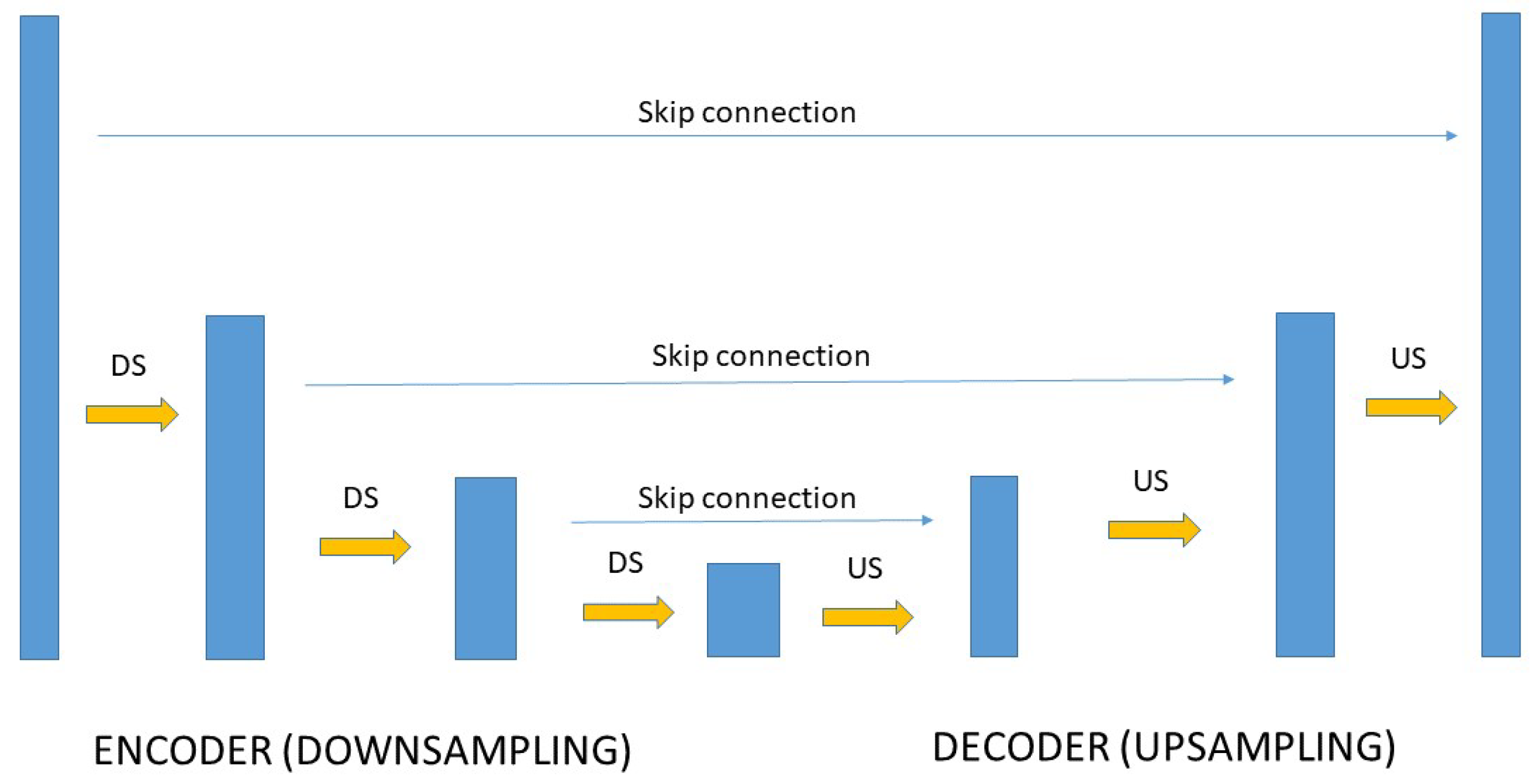
An example where the information retrieval and data fusion are combined through a single DL network was given in [32], where Meteosat Spinning Enhanced Visible and Infrared (SEVIRI) [33] geostationary satellite images were combined with rain gauges for the estimation of the amount of precipitation. In [32], a multiscale DL network of the U-Net type [34] combines spectral and spatial information from three selected SEVIRI channels at 8.7, 10.8, and 12.0 m with surface rain gauges. The U-Net architecture is a popular example of a Convolutional Neural Network (CNN), illustrated in Figure 1. We note that those SEVIRI channels are usable day and night and contain information on microphysical parameters relevant to precipitation processes [35]. The network simultaneously performs different tasks:
- Retrieval of the precipitation amount from SEVIRI channels trained on rain gauge data;
- Adaptive interpolation of rain gauge data;
- Data fusion of interpolated rain gauge data and satellite retrievals.
The resulting AI-based satellite/rain gauge precipitation estimates have recently been shown to be more accurate than the preceding state-of-the-art, that is traditional, non-AI-based radar/rain gauge precipitation estimates [36].
Another example of AI-based data fusion is the Multi-Instrument Inversion and Data Assimilation Preprocessing System (MIIDAPS-AI) [37]. MIIDAPS-AI provides an AI-based data fusion of microwave and infrared imagers and sounders and produces the analysis of a variety of atmospheric parameters. The algorithms for the data fusion of around ten satellite sensors was built by two people in less than ten months. The processing time was at least a factor 100 smaller than for a comparable non-AI-based system.
In [38], DL in combination with optical flow was used to detect convective initialization. This is an example of the use of DL to enhance an existing observation system, by extracting new information that was hitherto unexploited.
4.2. Nowcasting
For short forecast ranges typically up to 4–6 h in the future, the direct extrapolation of observations—referred to as nowcasting—is considered more accurate than an NWP forecast [39]. For satellite-based nowcasting, the extrapolation of satellite images with optical flow methods provided better skill scores than NWP models, in particular for phenomena dealing with clouds [40], e.g., surface radiation, heavy precipitation and thunderstorms. An example of the application of thunderstorm nowcasting is the use in aviation to avoid hazardous weather situations.
The nowcasting methods are expected to be significantly improved by combining different data sources, e.g., satellite images, radar, ground-based data and crowdsourced data. As a consequence, nowcasting deals with the challenge of big data and with shortcomings in the quality control and analysis of the value and weights of the different data sources, characterized by diverse origins, types, densities and reliability.
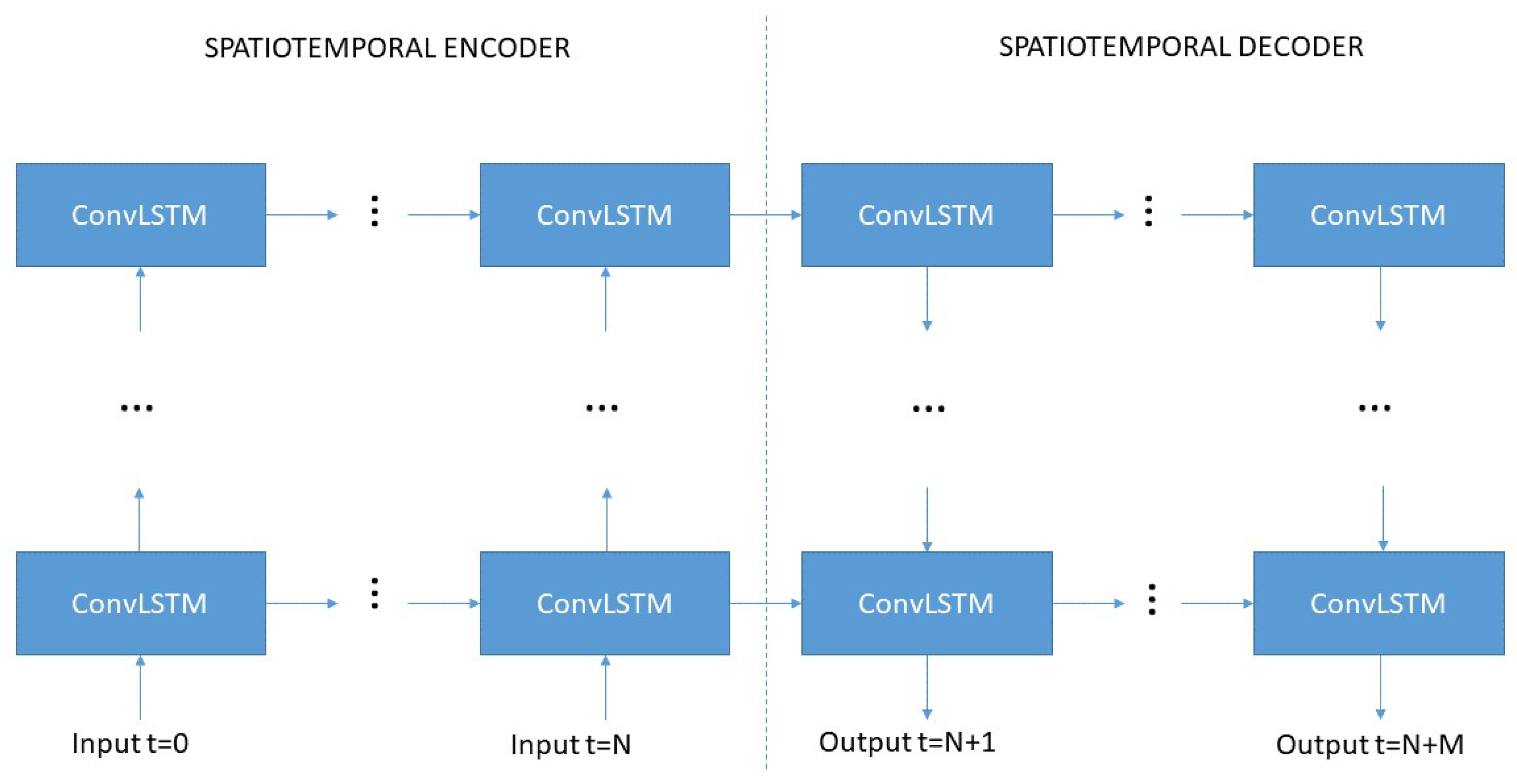
A DL-based architecture for nowcasting was first proposed in [41] and consists of an encoder–decoder architecture, where the encoder performs motion detection or a more complicated spatiotemporal analysis and the decoder performs motion extrapolation or a more complicated spatiotemporal forecasting. Both the encoder and the decoder used stacked ConvLSTM units, which were based on Long Short-Term Memory (LSTM) [42] recurrent neural networks for time forecasting and which have convolutional structures in both the input-to-state and the state-to-state transitions.
The stacked ConvLSTM architecture is illustrated in Figure 2.
In [43], a DL-based, purely data-driven nowcasting of precipitation using sequences of satellite and radar images as the input was presented. The DL network consists of an input spatial encoder, a middle temporal encoder based on ConvLSTMs and an output spatial aggregator. The network directly produces the probability distribution of the precipitation, i.e., a probabilistic precipitation nowcast, with forecast ranges up to 8 h. The performance of the DL nowcasting, compared to reference radar observations, is superior to a convection-permitting NWP with radar data assimilation. It is noteworthy that the DL nowcasting network of [43] thus outperforms the convection-permitting NWP model on its own grounds [13], namely the one of improved short-term precipitation forecast skill.
4.3. Pure AI Forecasting
As opposed to the conventional NWP approach [1], where observations are assimilated into an NWP model based on a physical modelling of the behaviour of the atmosphere, it is possible to completely replace the physical NWP model with a pure data-driven AI-based model without any a priori physical knowledge included [44]. In [45], it was demonstrated that a pure AI forecasting model can have comparable performance to a conventional NWP model, provided that the models have a comparable resolution. A bottleneck for the development of pure AI-based forecasts at a resolution and performance comparable to state-of-the-art operational NWP forecasts is the availability of sufficient training data [45]. The best practical results can therefore be expected from a combination of NWP and AI techniques [46]. This might also facilitate the acceptance of AI in a domain hitherto dominated by numerical (physical) modelling. In [47], a benchmark dataset for the evaluation of pure AI forecasting was provided. Pure AI forecasting is an area of active development. Recent examples were described in [48,49].
4.4. Process Parametrisation
When we stay in the context of conventional NWP models, Machine Learning (ML) can be used to improve the parametrisation of physical processes that are not explicitly resolved in the model [50,51,52,53]. Reference [50] dealt with a general framework on how parametrisations can learn from observations and targeted high-resolution simulations, with a focus on the parametrization of clouds and convection. Reference [51] focused on the Machine Learning (ML) parametrisation of moist convection, trained on the output of a conventional parametrization, and its behaviour when used in a climate model. Reference [52] derived a unified physics parametrization by minimising the forecast error over several days of prediction of a near-global cloud-resolving model. Reference [53] focused on the use of machine learning to derive the poorly known parts of a numerical Earth system model, in combination with physics-based modelling for the well-known parts of the model.
4.5. Hybrid AI NWP Forecasting
Given the limitation of the available training data, the best forecast performance can be expected from some form of combination of NWP and AI techniques. In August 2018, an AI weather forecast challenge was organised for the Beijing area [54], where the competing teams were asked to provide in real time the best 36 h forecasts for 2 m air temperature and relative humidity and 10 m wind speed, based on NWP model output and the surface observations of 10 automatic weather stations.
4.6. Postprocessing of NWP Output
A common way to improve the output of NWP models is to apply Model Output Statistics (MOS) [57] to correct the systematic errors of the NWP forecasts at different lead times. In [58], several Model Output Deep Learning (MODL) methods were investigated for the correction of temperature forecasts of the ECMWF NWP model. Averaged over a forecast range of 3–10 days, the original ECMWF temperature forecast error was 4 C, the conventional MOS temperature error 3 C, while the U-Net-based MODL error 2 C. An example of the use of the U-Net DL architecture for the postprocessing of cloud cover in an NWP model output was given in [59]. An example of the use of the DL architecture for the postprocessing of probabilistic NWP model ensemble forecasts was given in [60].
4.7. Multimodel Combination
NWP models are developed and run operationally at different centres around the world. The combination of multiple models can be an effective way to reduce the uncertainty of the forecasts, as demonstrated by using neural network techniques for hurricane intensity forecasts in [61]. An example of the use of DL techniques for the combination of multimodel outputs was given in [62].
4.8. Downscaling
Running high-resolution NWP models is costly in terms of computing resources. Convection-permitting NWP models at the global scale are currently at the limit of what is feasible using conventional NWP techniques. A possible solution is the use of DL techniques as described in [63]. Examples of the use of DL for the downscaling of wind fields were given in [64,65]. An example of the use of DL for the downscaling of temperature was given in [66].
4.9. Warnings for High-Impact Weather
4.10. Seasonal to Subseasonal Prediction
An important aspect of climate change is the so-called Arctic amplification (the Arctic temperature is rising twice as fast as the global temperature), which has important consequences for Northern Hemisphere midlatitude weather [69]. In particular, the temperature gradient between the Equator and the North Pole has reduced [70], which results in a weaker and wavier jet stream [71] and an increased occurrence of atmospheric blocking [72] and structural midlatitude drought [73]. In [74], it was shown that this mechanism is poorly represented in conventional weather and climate models and can better be captured by a Subseasonal-to-Seasonal (S2S) forecast system based on machine learning.
4.11. Decadal Climate Prediction
In [79], a CNN was successfully used to skilfully predict El Niño Southern Oscillation (ENSO) events with lead times up to one and a half years and with considerably better skill than dynamical physical forecast models. A particular problem for the training of decadal climate prediction is that the available observation period is too short to achieve proper training. In [79], this problem was solved through the use of transfer learning. First, the CNN was pretrained on model simulations; next, the training was refined using the available observations.
5. Benefits of New DL Techniques as Enhancements to Traditional NWP Methods
Traditional NWP data assimilation requires the development of a handcrafted observation parameter—hence a dedicated human development effort—for every observation type that is assimilated [1,5,6]. Moreover, it is common practice to use “data thinning” [80] prior to the assimilation, so that only a relatively small fraction of the available observations is actually used.
In contrast, DL methods “learn from data” [24]. This is efficient in terms of human effort. Furthermore, it allows learning hidden relations—which cannot be captured by physical models—and making use of the full potential of the available observations.
A prerequisite for the training of a DL method is the availability of a sufficient amount of training data. Today, not enough training data are available to train a “big bang” or “hard AI” method that can completely replace a traditional NWP method [45]. Instead, the available training data should be used to enhance existing NWP physical models, in a “residual learning” approach [81], where the DL network innovates on top of the physical model.
The state-of-the-art 4D-Var NWP data assimilation is an inverse modelling problem, which requires an iterative online cost function optimisation, which is costly in computing time [6,19]. The DL method’s training also requires a cost function optimisation, but in contrast to NWP data assimilation, this optimisation needs to be made only once, in an offline mode. A DL approach, once trained, can be operationally very efficient in computer time.
Probabilistic NWP forecasts are obtained by running multiple forecasts with slightly modified initial conditions. Running multiple forecasts is a “brute force” method, which is costly in computing time. A key advantage of DL is its flexibility. It can be trained for a deterministic forecast, as well as for probability density output [43], without the need to produce multiple integrations of a deterministic NWP or climate model.
6. Summary
In the past few decades, remarkable progress in weather forecast skill—with high societal benefits—has been achieved. The key technological advances underpinning this success have been the increase in computing power, the development of the 4D-Var data assimilation technique and the availability of global satellite observations for an increasing number of atmospheric parameters. AI and, in particular, DL hold great promise to become the new key technology that will further revolutionize operational weather forecasting in the years to come.
DL is data driven; this means that DL models are derived from large labelled datasets, requiring much less human development effort than traditional methods. As not enough labelled data are available to train a complete DL weather forecast model with a resolution comparable to current operational NWP models, the best results can be obtained from the “residual learning” approach, where a DL model innovates on top of an existing physics-based NWP model.
Traditional NWP models are demanding in terms of computing power, in particular as concerns the online data assimilation cost function optimisation and the need to run the model multiple times to obtain a probabilistic forecast. In contrast, DL models require a high computing power only during the offline training phase. In their online execution, they can be very efficient.
Traditional NWP models solve an initial value problem, where the knowledge of the current state of the atmosphere—based on observations—is combined with physics-based prognostic equations, which are solved iteratively forward in time. In the new DL approach, the traditional initial value problem can be replaced by an end-to-end trainable DL model, where the forecast step is included in the model optimisation. Such a DL model has the potential to be not only more efficient in terms of human development effort and computing power, but also more performant in terms of forecast quality.
7. The Way Forward
In order to exploit the clear potential benefits of the application of AI for weather and climate studies, a new generation of scientists needs to be trained, combining both domain knowledge in the Earth system sciences and specific AI expertise. AI should become a cornerstone of the weather and climate models of the future, such as the “DestinE” initiative. Operational weather and climate organisations are increasingly including the use of AI in their strategies. The number of workshops, benchmark datasets and journal Special Issues dedicated to the subject of AI for weather and climate application is increasing. It is very likely that within the next five to ten years, AI will become an indispensable part of state-of-the-art weather forecasting and climate monitoring and prediction. Techniques such as transfer learning and data augmentation, which have given a boost to many other applications, could accelerate the impact of AI techniques in climate and weather prediction and reduce the need for extra-large labelled datasets.
Author Contributions
S.D. had the initial idea and wrote the first version of this white paper. J.P.C., R.M. and A.M. provided improvements to the initial text. All authors read and agreed to the published version of the manuscript.
Funding
No dedicated funding was received for this paper.
Institutional Review Board Statement
Not applicable.
Informed Consent Statement
Not applicable.
Data Availability Statement
Not applicable.
Acknowledgments
The idea to write this paper originated at the first EUMETNET workshop on AI for weather and climate hosted at the RMIB in February 2020. EUMETNET is a grouping of 31 European National Meteorological Services that provides a framework to organise cooperative programmes among its Members in the various fields of basic meteorological activities. These activities include observing systems, data processing, basic forecasting products, research and development and training.
Conflicts of Interest
The authors declare no conflict of interest.
Abbreviations
The following abbreviations are used in this manuscript:
| AI | Artificial Intelligence |
| CM | Climate Monitoring |
| CPU | Central Processing Unit |
| DestinE | Destination Earth |
| DEP | Digital Europe Program |
| DL | Deep Learning |
| DP | Decadal Prediction |
| DT | Digital Twin |
| ECMWF | European Center for Mid-Range Weather Forecasting |
| GPU | Graphical Processing Unit |
| LSTM | Long Short-Term Memory |
| ML | Machine Learning |
| MLP | Multilayer Perceptron |
| MODL | Model Output Deep Learning |
| MOS | Model Output Statistics |
| NWP | Numerical Weather Prediction |
| RNN | Recurrent Neural Network |
| STAN | Spatiotemporal Attention Network |
| WF | Weather Forecast |
References
- Bauer, P.; Thorpe, A.; Brunet, G. The quiet revolution of numerical weather prediction. Nature 2015, 525, 47–55. [Google Scholar] [CrossRef]
- Edenhofer, O.; Pichs-Madruga, R.; Sokona, Y.; Farahani, E.; Kadner, S.; Seyboth, K.; Adler, A.; Baum, I.; Brunner, S.; Eickemeier, P.; et al. (Eds.) IPCC WGIII AR5 Summary for Policymakers; Cambridge University Press: Cambridge, UK; New York, NY, USA, 2014. [Google Scholar]
- Paris Agreement. In Report of the Conference of the Parties to the United Nations Framework Convention on Climate Change (21st Session, Dec. 2015: Paris); UNFCCC: Paris, France, 2015; Volume 4, p. 2017.
- Claeys, G.; Tagliapietra, S.; Zachmann, G. How to make the European Green Deal Work; Bruegel: Brussels, Belgium, 2019. [Google Scholar]
- Simmons, A.J.; Hollingsworth, A. Some aspects of the improvement in skill of numerical weather prediction. Q. J. R. Meteorol. Soc. 2002, 128, 647–677. [Google Scholar] [CrossRef]
- Rabier, F. Overview of global data assimilation developments in numerical weather-prediction centres. Q. J. R. Meteorol. Soc. 2005, 131, 3215–3233. [Google Scholar] [CrossRef]
- Huang, X.Y.; Xiao, Q.; Barker, D.M.; Zhang, X.; Michalakes, J.; Huang, W.; Henderson, T.; Bray, J.; Chen, Y.; Ma, Z.; et al. Four-dimensional variational data assimilation for WRF: Formulation and preliminary results. Mon. Weather Rev. 2009, 137, 299–314. [Google Scholar] [CrossRef] [Green Version]
- Ochotta, T.; Gebhardt, C.; Saupe, D.; Wergen, W. Adaptive thinning of atmospheric observations in data assimilation with vector quantization and filtering methods. Q. J. R. Meteorol. Soc. 2005, 131, 3427–3437. [Google Scholar] [CrossRef] [Green Version]
- About Our Forecasts-Operational Configurations of the ECMWF Integrated Forecasting System (IFS). Available online: https://www.ecmwf.int/en/forecasts/documentation-and-support (accessed on 22 February 2021).
- Archer, D.; Eby, M.; Brovkin, V.; Ridgwell, A.; Cao, L.; Mikolajewicz, U.; Caldeira, K.; Matsumoto, K.; Munhoven, G.; Montenegro, A.; et al. Atmospheric lifetime of fossil fuel carbon dioxide. Annu. Rev. Earth Planet. Sci. 2009, 37, 117–134. [Google Scholar] [CrossRef] [Green Version]
- Manabe, S.; Stouffer, R.J. Sensitivity of a global climate model to an increase of CO2 concentration in the atmosphere. J. Geophys. Res. Ocean. 2009, 85, 5529–5554. [Google Scholar] [CrossRef] [Green Version]
- Cullen, M.J.P.; Davies, T.; Mawson, M.H.; James, J.A.; Coulter, S.C.; Malcolm, A. An overview of numerical methods for the next generation UK NWP and climate model. Atmosphere-Ocean 1997, 35 (Suppl. 1), 425–444. [Google Scholar] [CrossRef]
- Clark, P.; Roberts, N.; Lean, H.; Ballard, S.P.; Charlton-Perez, C. Convection-permitting models: A step-change in rainfall forecasting. Meteorol. Appl. 2016, 23, 165–181. [Google Scholar] [CrossRef] [Green Version]
- Aligo, E.A.; Gallus, W.A.; Segal, M. On the impact of WRF model vertical grid resolution on Midwest summer rainfall forecasts. Weather Forecast. 2009, 24, 575–594. [Google Scholar] [CrossRef] [Green Version]
- Capecchi, V.; Antonini, A.; Benedetti, R.; Fibbi, L.; Melani, S.; Rovai, L.; Ricchi, A.; Cerrai, D. Assimilating X-and S-band Radar Data for a Heavy Precipitation Event in Italy. Water 2021, 13, 1727. [Google Scholar] [CrossRef]
- Maiello, I.; Gentile, S.; Ferretti, R.; Baldini, L.; Roberto, N.; Picciotti, E.; Alberoni, P.P.; Marzano, F.S. Impact of multiple radar reflectivity data assimilation on the numerical simulation of a flash flood event during the HyMeX campaign. Hydrol. Earth Syst. Sci. 2017, 21, 5459–5476. [Google Scholar] [CrossRef] [Green Version]
- Ricchi, A.; Bonaldo, D.; Cioni, G.; Carniel, S.; Miglietta, M.M. Simulation of a flash-flood event over the Adriatic Sea with a high-resolution atmosphere–ocean–wave coupled system. Sci. Rep. 2021, 11, 9388. [Google Scholar] [CrossRef] [PubMed]
- Zheng, Y.; Alapaty, K.; Herwehe, J.A.; Del Genio, A.D.; Niyogi, D. Improving high-resolution weather forecasts using the Weather Research and Forecasting (WRF) Model with an updated Kain–Fritsch scheme. Mon. Weather Rev. 2016, 144, 833–860. [Google Scholar] [CrossRef]
- Bauer, P.; Dueben, P.D.; Hoefler, T.; Quintino, T.; Schulthess, T.C.; Wedi, N.P. The digital revolution of Earth-system science. Nat. Comput. Sci. 2021, 1, 104–113. [Google Scholar] [CrossRef]
- Palmer, T.; Stevens, B. The scientific challenge of understanding and estimating climate change. Proc. Natl. Acad. Sci. USA 2019, 116, 24390–24395. [Google Scholar] [CrossRef] [Green Version]
- Robertson, A.W.; Kumar, A.; Peña, M.; Vitart, F. Improving and Promoting Subseasonal to Seasonal Prediction. Bull. Am. Meteorol. Soc. 2015, 96, ES49–ES53. [Google Scholar] [CrossRef]
- Meehl, G.A.; Goddard, L.; Boer, G.; Burgman, R.; Branstator, G.; Cassou, C.; Corti, S.; Danabasoglu, G.; Doblas-Reyes, F.; Hawkins, E.; et al. Decadal Climate Prediction: An Update from the Trenches. Bull. Am. Meteorol. Soc. 2014, 95, 243–267. [Google Scholar] [CrossRef] [Green Version]
- Bauer, P.; Stevens, B.; Hazeleger, W. A digital twin of Earth for the green transition. Nat. Clim. Chang. 2021, 11, 80–83. [Google Scholar] [CrossRef]
- LeCun, Y.; Bengio, Y.; Hinton, G. Deep learning. Nature 2015, 521, 436–444. [Google Scholar] [CrossRef]
- Shrestha, A.; Mahmood, A. Review of deep learning algorithms and architectures. IEEE Access 2019, 7, 53040–53065. [Google Scholar] [CrossRef]
- Reichstein, M.; Camps-Valls, G.; Stevens, B.; Jung, M.; Denzler, J.; Carvalhais, N. Deep learning and process understanding for data-driven Earth system science. Nature 2008, 566, 195–204. [Google Scholar] [CrossRef] [PubMed]
- Guo, H.; Fu, W.; Liu, G. European Earth Observation Satellites. In Scientific Satellite and Moon-Based Earth Observation for Global Change; Springer: Singapore, 2019; pp. 97–135. [Google Scholar]
- Zheng, F.; Tao, R.; Maier, H.R.; See, L.; Savic, D.; Zhang, T.; Chen, Q.; Assumpção, T.H.; Yang, P.; Heidari, B.; et al. Crowdsourcing methods for data collection in geophysics: State of the art, issues, and future directions. Rev. Geophys. 2018, 56, 698–740. [Google Scholar] [CrossRef]
- Boukabara, S.A.; Krasnopolsky, V.; Stewart, J.Q.; Maddy, E.S.; Shahroudi, N.; Hoffman, R.N. Leveraging Modern Artificial Intelligence for Remote Sensing and NWP: Benefits and Challenges. Bull. Am. Meteorol. Soc. 2019, 100, ES473–ES491. [Google Scholar] [CrossRef]
- Arcucci, R.; Zhu, J.; Hu, S.; Guo, Y.K. Deep data assimilation: Integrating deep learning with data assimilation. Appl. Sci. 2021, 11, 1114. [Google Scholar] [CrossRef]
- Ghamisi, P.; Rasti, B.; Yokoya, N.; Wang, Q.; Hofle, B.; Bruzzone, L.; Bovolo, F.; Chi, M.; Anders, K.; Gloaguen, R.; et al. Multisource and multitemporal data fusion in remote sensing: A comprehensive review of the state-of-the-art. IEEE Geosci. Remote Sens. Mag. 2019, 7, 6–39. [Google Scholar] [CrossRef] [Green Version]
- Moraux, A.; Dewitte, S.; Cornelis, B.; Munteanu, A. Deep Learning for Precipitation Estimation from Satellite and Rain Gauges Measurements. Remote Sens. 2019, 11, 2463. [Google Scholar] [CrossRef] [Green Version]
- Schmetz, J.; Pili, P.; Tjemkes, S.; Just, D.; Kerkmann, J.; Rota, S.; Ratier, A. An introduction to Meteosat second generation (MSG). Bull. Am. Meteorol. Soc. 2002, 83, 977–992. [Google Scholar] [CrossRef]
- Ronneberger, O.; Fischer, P.; Brox, T. U-net: Convolutional networks for biomedical image segmentation. In International Conference on Medical Image Computing and Computer-Assisted Intervention; Springer: Cham, Switzerland, 2015; pp. 234–241. [Google Scholar]
- Rosenfeld, D.; Lensky, I.M. Satellite-based insights into precipitation formation processes in continental and maritime convective clouds. Bull. Am. Meteorol. Soc. 1998, 79, 2457–2476. [Google Scholar] [CrossRef] [Green Version]
- Moraux, A.; Dewitte, S.; Cornelis, B.; Munteanu, A. A Deep Learning for Multimodal Method for Precipitation Estimation. Remote Sens. 2021, submitted. [Google Scholar]
- Boukabara, S.A.; Maddy, E.; Shahroudi, N.; Hoffman, R.N.; Connor, T.; Upton, S.; Ten Hoeve, J.E. Artificial Intelligence (AI) Techniques to Enhance Satellite Data Use for Nowcasting and NWP/Data Assimilation. In Proceedings of the 100th American Meteorological Society Annual Meeting, AMS, Boston, MA, USA, 12–16 January 2020. [Google Scholar]
- Schön, C.; Dittrich, J.; Müller, R. The error is the feature: How to forecast lightning using a model prediction error. In Proceedings of the 25th ACM SIGKDD International Conference on Knowledge Discovery and Data Mining, Anchorage, AK, USA, 4–8 August 2019; pp. 2979–2988. [Google Scholar]
- Haiden, T.; Kann, A.; Pistotnik, G.; Stadlbacher, K.; Wittmann, C. Integrated Nowcasting through Comprehensive Analysis (INCA)—System Description; ZAMG Rep, 61; ZAMG: Vienna, Austria, 2009. [Google Scholar]
- Urbich, I.; Bendix, J.; Müller, R. Development of a Seamless Forecast for Solar Radiation Using ANAKLIM++. Remote Sens. 2020, 12, 3672. [Google Scholar] [CrossRef]
- Shi, X.; Chen, Z.; Wang, H.; Yeung, D.Y.; Wong, W.K.; Woo, W.C. Convolutional LSTM network: A machine learning approach for precipitation nowcasting. In Proceedings of the 28th International Conference on Neural Information Processing Systems, Montreal, QC, Canada, 7–12 December 2015; Volume 1, pp. 802–810. [Google Scholar]
- Hochreiter, S.; Schmidhuber, J. Long short-term memory. Neural Comput. 1997, 9, 1735–1780. [Google Scholar] [CrossRef]
- Kaae Sønderby, C.; Espeholt, L.; Heek, J.; Dehghani, M.; Oliver, A.; Salimans, T.; Agrawal, S.; Hickey, J.; Kalchbrenner, N. MetNet: A Neural Weather Model for Precipitation Forecasting. arXiv 2020, arXiv:2003.12140. [Google Scholar]
- Scher, S. Toward data-driven weather and climate forecasting: Approximating a simple general circulation model with deep learning. Geophys. Res. Lett. 2018, 45, 12–616. [Google Scholar] [CrossRef] [Green Version]
- Dueben, P.D.; Bauer, P. Challenges and design choices for global weather and climate models based on machine learning. Geosci. Model Dev. 2018, 11, 3999–4009. [Google Scholar] [CrossRef] [Green Version]
- Schultz, M.G.; Betancourt, C.; Gong, B.; Kleinert, F.; Langguth, M.; Leufen, L.H.; Mozaffari, A.; Stadtler, S. Can deep learning beat numerical weather prediction? Philos. Trans. R. Soc. A 2021, 379, 20200097. [Google Scholar] [CrossRef] [PubMed]
- Rasp, S.; Dueben, P.D.; Scher, S.; Weyn, J.A.; Mouatadid, S.; Thuerey, N. WeatherBench: A benchmark dataset for data-driven weather forecasting. J. Adv. Model. Earth Syst. 2020, 12, e2020MS002203. [Google Scholar] [CrossRef]
- Kim, K.S.; Lee, J.B.; Roh, M.I.; Han, K.M.; Lee, G.H. Prediction of Ocean Weather Based on Denoising AutoEncoder and Convolutional LSTM. J. Mar. Sci. Eng. 2020, 8, 805. [Google Scholar] [CrossRef]
- Zheng, G.; Li, X.; Zhang, R.H.; Liu, B. Purely satellite data–driven deep learning forecast of complicated tropical instability waves. Sci. Adv. 2020, 6, 1482. [Google Scholar] [CrossRef] [PubMed]
- Schneider, T.; Lan, S.; Stuart, A.; Teixeira, J. Earth system modeling 2.0: A blueprint for models that learn from observations and targeted high resolution simulations. Geophys. Res. Lett. 2017, 44, 12–396. [Google Scholar] [CrossRef] [Green Version]
- O’Gorman, P.A.; Dwyer, J.G. Using machine learning to parameterize moist convection: Potential for modeling of climate, climate change, and extreme events. J. Adv. Model. Earth Syst. 2018, 10, 2548–2563. [Google Scholar] [CrossRef] [Green Version]
- Brenowitz, N.D.; Bretherton, C.S. Prognostic validation of a neural network unified physics parameterization. Geophys. Res. Lett. 2018, 45, 6289–6298. [Google Scholar] [CrossRef]
- Brajard, J.; Charantonis, A.; Sirven, J. Representing ill-known parts of a numerical model using a machine learning approach. arXiv 2019, arXiv:1903.07358. [Google Scholar]
- Ji, L.; Wang, Z.; Chen, M.; Fan, S.; Wang, Y.; Shen, Z. How much can AI techniques improve surface air temperature forecast? A report from AI Challenger 2018 Global Weather Forecast Contest. J. Meteorol. Res. 2019, 33, 989–992. [Google Scholar] [CrossRef]
- Li, Y.; Lang, J.; Ji, L.; Zhong, J.; Wang, Z.; Guo, Y.; He, S. Weather Forecasting Using Ensemble of Spatial-Temporal Attention Network and Multi-Layer Perceptron. Asia-Pac. J. Atmos. Sci. 2020, 57, 533–546. [Google Scholar] [CrossRef]
- Wang, B.; Lu, J.; Yan, Z.; Luo, H.; Li, T.; Zheng, Y.; Zhang, G. Deep uncertainty quantification: A machine learning approach for weather forecasting. In Proceedings of the 25th ACM SIGKDD International Conference on Knowledge Discovery and Data Mining, Anchorage, AK, USA, 4–8 August 2019; pp. 2087–2095. [Google Scholar]
- Glahn, H.R.; Lowry, D.A. The use of model output statistics (MOS) in objective weather forecasting. J. Appl. Meteorol. 1972, 11, 1203–1211. [Google Scholar] [CrossRef] [Green Version]
- Chen, K.; Wang, P.; Yang, X.; Zhang, N.; Wang, D. A Model Output Deep Learning Method for Grid Temperature Forecasts in Tianjin Area. Appl. Sci. 2020, 10, 5808. [Google Scholar] [CrossRef]
- Dupuy, F.; Mestre, O.; Serrurier, M.; Bakkay, M.C.; Burdá, V.K.; Cabrera-Gutiérrez, N.C.; Bakkay, M.C.; Jouhaud, J.C.; Mader, M.A.; Oller, G. ARPEGE cloud cover forecast post-processing with convolutional neural network. Weather Forecast. 2020, 36, 567–586. [Google Scholar] [CrossRef]
- Grönquist, P.; Yao, C.; Ben-Nun, T.; Dryden, N.; Dueben, P.; Li, S.; Hoefler, T. Deep Learning for Post-Processing Ensemble Weather Forecasts. Philos. Trans. R. Soc. A 2020, 379, 20200092. [Google Scholar] [CrossRef]
- Ghosh, T.; Krishnamurti, T.N. Improvements in hurricane intensity forecasts from a multimodel superensemble utilizing a generalized neural network technique. Weather Forecast. 2018, 33, 873–885. [Google Scholar] [CrossRef]
- Kirkwood, C.; Economou, T.; Odbert, H.; Pugeault, N. A framework for probabilistic weather forecast post-processing across models and lead times using machine learning. Philos. Trans. R. Soc. A 2020, 379, 20200099. [Google Scholar] [CrossRef] [PubMed]
- Rodrigues, E.R.; Oliveira, I.; Cunha, R.; Netto, M. DeepDownscale: A deep learning strategy for high-resolution weather forecast. In Proceedings of the 2018 IEEE 14th International Conference on e-Science (e-Science), Amsterdam, The Netherlands, 29 October–1 November 2018; pp. 415–422. [Google Scholar]
- Li, L. Geographically weighted machine learning and downscaling for high-resolution spatiotemporal estimations of wind speed. Remote Sens. 2019, 11, 1378. [Google Scholar] [CrossRef] [Green Version]
- Höhlein, K.; Kern, M.; Hewson, T.; Westermann, R. A comparative study of convolutional neural network models for wind field downscaling. Meteorol. Appl. 2020, 27, e1961. [Google Scholar] [CrossRef]
- Sekiyama, T.T. Statistical Downscaling of Temperature Distributions from the Synoptic Scale to the Mesoscale Using Deep Convolutional Neural Networks. arXiv 2020, arXiv:2007.10839. [Google Scholar]
- Chattopadhyay, A.; Nabizadeh, E.; Hassanzadeh, P. Analog forecasting of extreme-causing weather patterns using deep learning. J. Adv. Model. Earth Syst. 2019, 12, e2019MS001958. [Google Scholar] [CrossRef] [PubMed]
- Chattopadhyay, A.; Hassanzadeh, P.; Pasha, S. Predicting clustered weather patterns: A test case for applications of convolutional neural networks to spatiotemporal climate data. Sci. Rep. 2020, 10, 1317. [Google Scholar] [CrossRef]
- Cohen, J.; Screen, J.A.; Furtado, J.C.; Barlow, M.; Whittleston, D.; Coumou, D.; Francis, J.; Dethloff, K.; Entekhabi, D.; Overl, J.; et al. Recent Arctic amplification and extreme mid-latitude weather. Nat. Geosci. 2014, 7, 627–637. [Google Scholar] [CrossRef] [Green Version]
- Overl, J.E.; Dethloff, K.; Francis, J.A.; Hall, R.J.; Hanna, E.; Kim, S.J.; Screen, J.A.; Shepherd, T.G.; Vihma, T. Nonlinear response of mid-latitude weather to the changing Arctic. Nat. Clim. Chang. 2016, 6, 992–999. [Google Scholar] [CrossRef] [Green Version]
- Francis, J.A.; Vavrus, S.J. Evidence for a wavier jet stream in response to rapid Arctic warming. Environ. Res. Lett. 2015, 10, 014005. [Google Scholar] [CrossRef]
- Hanna, E.; Cropper, T.E.; Hall, R.J.; Cappelen, J. Greenland Blocking Index 1851–2015: A regional climate change signal. Int. J. Climatol. 2016, 36, 4847–4861. [Google Scholar] [CrossRef] [Green Version]
- Routson, C.C.; McKay, N.P.; Kaufman, D.S.; Erb, M.P.; Goosse, H.; Shuman, B.N.; Rodysill, J.R.; Ault, T. Mid-latitude net precipitation decreased with Arctic warming during the Holocene. Nature 2019, 568, 83–87. [Google Scholar] [CrossRef] [PubMed]
- Cohen, J.; Coumou, D.; Hwang, J.; Mackey, L.; Orenstein, P.; Totz, S.; Tziperman, E. S2S reboot: An argument for greater inclusion of machine learning in subseasonal to seasonal forecasts. Wiley Interdiscip. Rev. Clim. Chang. 2019, 10, e00567. [Google Scholar] [CrossRef] [Green Version]
- Hwang, J.; Orenstein, P.; Cohen, J.; Pfeiffer, K.; Mackey, L. Improving subseasonal forecasting in the western US with machine learning. In Proceedings of the 25th ACM SIGKDD International Conference on Knowledge Discovery and Data Mining, Anchorage, AK, USA, 4–8 August 2019; pp. 2325–2335. [Google Scholar]
- He, S.; Li, X.; DelSole, T.; Ravikumar, P.; Banerjee, A. Sub-Seasonal Climate Forecasting via Machine Learning: Challenges, Analysis, and Advances. arXiv 2020, arXiv:2006.07972. [Google Scholar]
- Weyn, J.A.; Durran, D.R.; Caruana, R. Improving data-driven global weather prediction using deep convolutional neural networks on a cubed sphere. J. Adv. Model. Earth Syst. 2020, 12, e2020MS002109. [Google Scholar] [CrossRef]
- Weyn-Vanhentenryck, J. Sub-Seasonal Forecasting Using Large Ensembles of Data-Driven Global Weather Prediction Models. Doctoral Dissertation, University of Washington, Seattle, WA, USA, 2020. [Google Scholar]
- Ham, Y.G.; Kim, J.H.; Luo, J.J. Deep learning for multi-year ENSO forecasts. Nature 2019, 573, 568–572. [Google Scholar] [CrossRef] [PubMed]
- Bauer, P.; Buizza, R.; Cardinali, C.; Thépaut, J.-N. Impact of singular-vector-based satellite data thinning on NWP. Q. J. R. Meteorol. Soc. 2011, 137, 286–302. [Google Scholar] [CrossRef]
- He, K.; Zhang, X.; Ren, S.; Sun, J. Deep residual learning for image recognition. In Proceedings of the IEEE Conference on Computer Vision and Pattern Recognition, Las Vegas, NV, USA, 27–30 June 2016; pp. 770–778. [Google Scholar]
Figure 1.
Illustration of the U-Net architecture, consisting of a downsampling encoder network followed by an upsampling decoder network. DS = DownSampling, US = UpSampling, blue rectangles = convolutional layers. Horizontal arrows connecting the encoder with the decoder at a particular resolution indicate skip connections, allowing for the propagation of context information from lower- to higher-resolution layers. The decoder path looks more or less symmetric with respect to the decoder path, and a U-shaped architecture is obtained.

Figure 2.
Illustration of the stacked ConvLSTM architecture. ConvLSTM is a type of recurrent neural network for spatiotemporal prediction that has convolutional structures in both the input-to-state and state-to-state transitions. The ConvLSTM determines the future state of a given cell in the grid by the inputs and past states of its local neighbours.

Publisher’s Note: MDPI stays neutral with regard to jurisdictional claims in published maps and institutional affiliations. |
© 2021 by the authors. Licensee MDPI, Basel, Switzerland. This article is an open access article distributed under the terms and conditions of the Creative Commons Attribution (CC BY) license (https://creativecommons.org/licenses/by/4.0/).
Share and Cite
MDPI and ACS Style
Dewitte, S.; Cornelis, J.P.; Müller, R.; Munteanu, A. Artificial Intelligence Revolutionises Weather Forecast, Climate Monitoring and Decadal Prediction. Remote Sens. 2021, 13, 3209. https://0-doi-org.brum.beds.ac.uk/10.3390/rs13163209
AMA Style
Dewitte S, Cornelis JP, Müller R, Munteanu A. Artificial Intelligence Revolutionises Weather Forecast, Climate Monitoring and Decadal Prediction. Remote Sensing. 2021; 13(16):3209. https://0-doi-org.brum.beds.ac.uk/10.3390/rs13163209
Chicago/Turabian StyleDewitte, Steven, Jan P. Cornelis, Richard Müller, and Adrian Munteanu. 2021. "Artificial Intelligence Revolutionises Weather Forecast, Climate Monitoring and Decadal Prediction" Remote Sensing 13, no. 16: 3209. https://0-doi-org.brum.beds.ac.uk/10.3390/rs13163209
Note that from the first issue of 2016, this journal uses article numbers instead of page numbers. See further details here.