A Satellite-USV System for Persistent Observation of Mesoscale Oceanographic Phenomena

Abstract

Traditional tools and methodologies for mesoscale observation of oceanographic phenomena are limited by under-sampling and data latency. In this article we evaluate three different scenario variants of an architecture for how heterogeneous sensor nodes can be integrated with satellite remote sensing. Independent space and marine sensing platforms are interconnected either directly or by means of a ground-based mission control center responsible for data processing, relay, and coordination of the assets. A wave-propelled unmanned surface vehicle (USV) persistently collects in situ data of the targeted phenomenon. In two variants of the architecture, a dedicated small satellite acts as a sensor node, a data processing facility and a communication node. We have used a System-of-Systems (SoS) modeling approach coupled with operational simulations in different locations on Earth, in order to support the proposed methodology and investigate quantitatively the reduction the data latency to end-users. Through a combination of field experiments and simulations we estimate how the different scenarios perform with respect to providing remote sensing data that are used to create a measurement and navigation plan for the autonomous vessel.

1. Introduction and Motivation

Human activity near and in oceans is strongly affecting our environment through the warming of the planet and increased eutrophication, causing substantial loss of sea-ice in the Arctic region [1], and it represents a profound threat to biodiversity. With a focus on the ocean as the primary sink for greenhouse gases, ocean science and the study of climate change has become critical to understanding our planet [2]. In particular, continuous observation of oceanographic phenomena as a stepping stone for understanding the impact of human activity on the world’s oceans is hampered by under-sampling and data latency. Unlike the atmosphere, the ocean is not continuously monitored or sampled, so the only way to learn its dynamic processes is to collect measurements with boats or diving platforms. However, such systems are expensive, and by only providing a glimpse of large phenomena cause short-term events to remain undetected. Current monitoring methodologies rely on both terrestrial and space-based remote sensing platforms. While most common terrestrial platforms and sensors are often constrained by proximity to ship or shore and by limited onboard energy, ocean color remote sensing based on optical imagery from space is limited by cloud coverage and weather phenomena.

The frequency of Harmful Algae Blooms (HABs) is increasing in step with increased human activity and eutrophication, and depending on the type of bloom, in some cases with the increased temperature of the oceans ([3], p. 17). HABs occur in oceans and lakes and can be highly toxic to aquatic and non-aquatic life or cause harmful effects by anoxia (oxygen depletion). These effects reduce the water quality that leads to significant recreational, economic, and ecological impacts [3]. Because the HABs typically occur in dynamic and optically complex water systems, and space-based remote sensing systems are desired to provide radiometry services multiple times a day [4]. Accordingly, the International Ocean Color Coordinating Group (IOCCG) state that "it is necessary to take a multi-layered approach to HAB studies, amalgamating information from multiple satellites, multiple sensors, and multiple adjunctive data sources to form a multidimensional understanding of the nature and dynamics of HABs ([3], p. 11)". Global environmental changes happen at large temporal and spatial scales. The study of phenomena evolving at smaller scales can provide valuable insights and enhance our understanding of the global, slow-changing dynamics of our planet.

The mesoscale variability (<1000 ${\mathrm{km}}^2$) can be best observed with mobile platforms that can sample a wide range of properties such as chlorophyll concentration, oxygen concentration, biomass, anthropogenic runoffs, temperature, salinity, vertical current structure, seafloor topography, and turbulence. Unmanned vehicles (such as Unmanned Underwater Vehicle (UUV), Unmanned Surface Vehicle (USV), Unmanned Aerial Vehicles (UAV)) are flexible assets that can individually observe and acquire data from various target areas [5]. However, no single platform is ideal for full coverage of oceanographic mesoscale phenomena [3]. Furthermore, to gain useful insights based on observations from different assets, they should be coordinated to observe the same patch of the ocean near-simultaneously, within time scales that fit the observed phenomena, i.e., synoptic observations [6]. The physical and operational diversity across such mobile platforms may result in complementary spatial and temporal sampling capabilities.

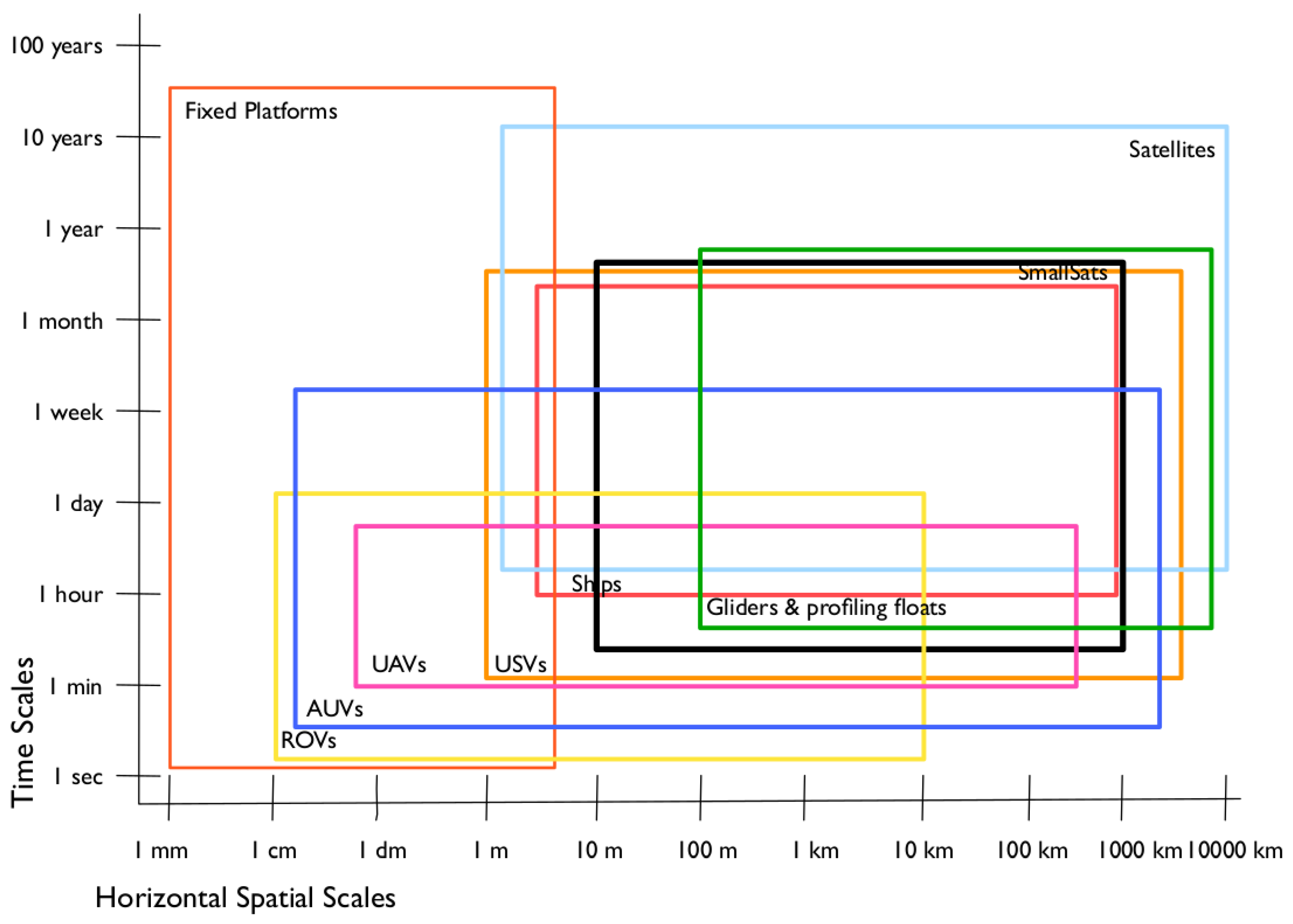
Figure 1 from [7] shows spatial and temporal scales of the most common marine and aerial systems employed in ocean studies. Small satellites and gliders operate at scales that mostly overlap in space and time and can as such enable synoptic measurements of the same phenomena. The cooperation of both systems indicates coverage of phenomena in the range of 100 m to 1000 km in space, from hours up to one year in time. Ship-based ocean observation also involves similar scales and points to well-consolidated methods ocean studies have relied on in recent decades. However, these involve higher operational cost and risk (for example, personnel costs, humans exposed to harsh environments) and, most importantly, they cannot scale across space and time and are therefore not suitable for the study of slow-changing oceanographic phenomena. Combining multiple different autonomous agents in a heterogeneous ocean sampling network has been demonstrated [8,9,10] to increase the amount of information and, therefore, the observation quality of physical phenomena beyond what each platform can achieve individually.

Sea gliders, both on the surface and sub-surface, are extensively employed as ocean observation platforms [11,12,13] because of their extended operational autonomy. Some works show the possibility to utilize such platforms to validate satellites measurements [14,15]. Nevertheless, the current state of the art lacks detailed modeling of marine operations in which the science-driven objectives for unmanned assets are based on processed data from small satellites.

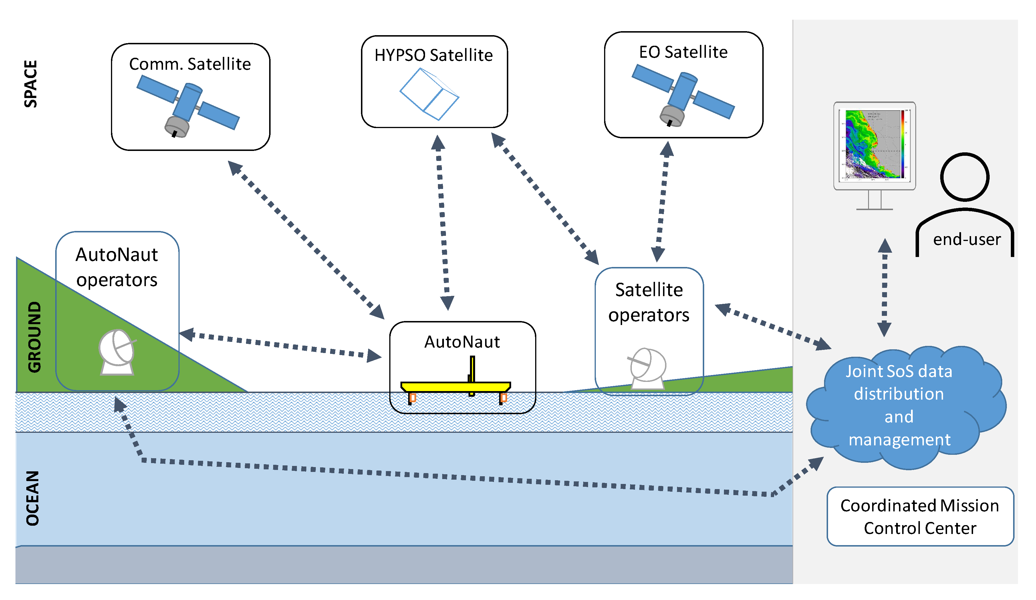
In this paper, we discuss how to enhance the study of oceanographic phenomena using satellites together with in situ terrestrial assets, as compared to using each platform independently. The proposed architecture is composed of a space segment with a mission-specific small satellite and "traditional" Earth Observation (EO) satellite data, a ground mission control center, and a long-endurance wave-propelled USV, as shown in Figure 2. The satellite offers an overview of an area where the sea glider collects detailed in situ measurements and transmits them to shore. In one variant of the system architecture, we make use of EO-data from existing satellites, whereas in the two other variants we model how the architecture would benefit from using a dedicated small satellite, such as the HYPerspectral small Satellite for Oceanographic observations (HYPSO)-1 satellite developed at Norwegian University of Science and Technology (NTNU).

The sea surface glider considered in this work is the AutoNaut, a commercially available wave-propelled USV equipped with a passive propulsion system that converts wave energy into forward thrust, see Figure 3.

To best exploit the capabilities of each asset, we propose a method for optimizing the information flow between the nodes of the architecture. We have employed a System-of-Systems (SoS) approach [16] for modeling and development and the solution presented can be classified as an acknowledged SOS. The use of an SOS approach has already been applied to other studies involving unmanned vehicles [17,18,19]. In particular, Reference [20] describes the application of an SOS approach for the detection and monitoring of forest fires involving forest-based infrared sensors, CubeSats providing early warning and communication services, and UAVs for high-resolution mapping. In our work, the acknowledged SOS has recognized objectives, providing a better information system for observing mesoscale phenomena, dedicated management, the research team, but the Constituent Systems (CS) have different development lifecycles, individual objectives, and a need for coordinating interfaces and operations to achieve the common goals. The authors postulate that architectures promoting tight cooperation between satellites and surface marine vehicles can improve the observation of oceanographic mesoscale phenomena and contribute to increasing the data available on HABs, both qualitatively and quantitatively, and provided data of a higher value and timeliness to end-users. Our analysis shows that while integrating existing systems will provide added information with little effort, making use of new tailor-made assets such as small satellites will improve the timeliness and the adaptivity of the observational system because the users can select their Area of Interests (AoIs) to a greater extent than currently possible.

The paper is structured as follows: In Section 2 we describe approaches for persistent observation of oceanographic phenomena, in Section 3 the constituent systems and scenarios are presented, followed by the methods applied in Section 4. In Section 5 we present the results. We present a discussion in Section 6. Finally, in Section 7, we summarize our findings and suggest areas for future studies.

2. Using Robotic Platforms to Support the Persistent Observation of Oceanographic Phenomena

The oceans are continuously surveyed on a global scale by remote sensing satellite systems like Copernicus [21,22], and even systems like Landsat provide data products, including monitoring of inland waters [23]. In addition, oceans are populated with measurement buoys (drifters) that continuously sample their surrounding environment and transmit collected data to shore for further analysis and processing [24]. Constrained by fixed position, short sensor range, lagrangian motion or limited payload energy, the network created by remote sensing buoys is expanded by remotely controlled platforms able to exploit the environment to achieve an intended navigational behavior [11,12,13,25]. These platforms are usually equipped with a wide-range sensor suite [26] that samples both near-surface atmospheric parameters (such as wind speed, pressure, temperature) [27] and features of the upper water column (for example, water salinity and temperature, sea currents, oxygen concentration) [28]. From ecological and biological perspectives, such systems are able to quantify natural phenomena related to animal primary productivity (by collecting chlorophyll and Dissolved Organic Matter (DOM) concentration), to assess the health of the ecosystem [29] (such as algal blooms, toxins concentration) or to study fish behavior and migrations via acoustic hydrophones [30], for example. Enhanced endurance and bigger payloads come, however, with a number of challenges related to the maneuverability and operational capabilities of such platforms, as described in Section 3.4.1.

The control of such robotic systems and the communication with them are challenging tasks due to the unpredictability of the environment. Goal-driven intent for scientific measurements will require careful balancing between the value of information related to the observed phenomenon and the ability to be at the right place at the right time. Moreover, communication challenges such as the limited bandwidth of satellite links influence the ability to provide valuable data to shore.

In Reference [15], a Wave Glider is used to persistently collect chlorophyll data for several months and validate satellite measurements. This work demonstrates that in situ measurements provided by long-endurance marine systems can be used, in combination with satellite observations, to provide a better understanding of the natural phenomena and climate changes of the planet. The Wave Glider was also used to validate winds measured by satellites in orbit [14] that use microwave sensors to observe the sea surface backscatter. Despite the important contributions of these works, their main objective was to validate quantitatively and qualitatively the existing satellite-based ocean monitoring methods. In Reference [31], an HAB detection system is proposed using existing satellites (MODIS Aqua and Terra, NASA) and gives some indications on how predictions of HAB can be carried out. The 2021 IOCCG report [3] provides more examples of HAB warning systems and how the data can be collected.

Our work addresses the observation of mesoscale phenomena in the short time range, i.e., phenomena detection from satellite and its in situ observation using terrestrial assets within the time scale of the phenomenon itself. Communication latency is assessed with simulations that provide insight on the spatial and temporal coordination that is needed among the involved assets. This coordination can increase the quality and amount of collected data and contribute to our understanding of the targeted phenomena.

3. System and Scenario Description

To overcome the limitations affecting current ocean observation systems, we advocate the development of integrated systems harvesting the specific benefits from each sensor platform. One of the current limitations in space-based remote sensing is that several maritime areas of scientific and economic interests are not covered well enough. Examples are the Norwegian sea and Arctic areas, the coast of Chile, Canadian waters, and areas in Scotland because of aquaculture installations [3]. Small satellites in Low Earth Orbit (LEO) equipped with instruments selected for each mission and use case can target specific AOIs with greater spectral and spatial resolution than large EO satellites at higher altitudes. The temporal resolution can also be determined by the user to a greater extent, by scheduling observations on demand and by selecting an orbit suitable for the AOI, such as polar orbits for Arctic areas.

The following sections describe the constituent systems in our SOS shown in Figure 2 and the scenarios foreseen to support the collection of HAB data and other oceanographic data.

The system consists of a space segment and a ground segment. The ground segment includes the wave-propelled USV AutoNaut, ground stations to communicate with the satellite, and a Coordinated Mission Control Center (CMCC). Note that there is a clear distinction between the ground stations and the CMCC; the ground stations encompass the antenna and infrastructure needed to establish the radio link to the satellite, while the operator is located at the CMCC.

3.1. The HYPSO Satellite and Ground Segment

The small satellite HYPSO is a 6U CubeSat equipped with a HyperSpectral Imager (HSI) payload featuring onboard processing of hyperspectral data based on a push-broom acquisition of data to support coordinated missions with unmanned vehicles [32]. The HSI telescope uses a Commercial-Off-The-Shelf (COTS) image sensor, COTS optical components, and in-house designed machined interfaces [33]. The design results in an unbinned Signal-to-Noise Ratio (SNR) of 180, detects wavelengths between 400–800 nm with a Full-Width at Half-Maximum (FWHM) of approximately $4 \mathrm{nm}$. The onboard processing unit is built on a Zynq-7030 Xilinx PicoZed System-on-a-Chip with a Field Programmable Gate Array (FPGA) and a two-core ARM processor. This processing unit provides a configurable platform for onboard processing and software, which can be tailored to suit the mission’s needs while in orbit. The FPGA enables rapid processing of large datasets, such as the hyperspectral data, and it utilizes CCSDS-123 lossless compression for image processing [34]. The configurable onboard processing of images can provide target detection and classification services to direct unmanned asset data collection. In addition, the HYPSO-1 CubeSat features an S-band radio link, a UHF radio link, and an Attitude Determination and Control System (ADCS) that allows for slew maneuvers to increase the SNR and improve the ground sampling distance [32].

While HYPSO-1 features a high spectral resolution, its spectral range and observations are limited by cloud cover, and payload operating time is limited by energy constraints. There is a plan to complement HYPSO-1 with more satellites carrying an upgraded payload to improve operational availability.

The space segment also includes commercially available communication systems that may be compatible with those onboard the AutoNaut. The ground segment supporting the HYPSO-1 spacecraft consists of commercially available ground communication services and an in-house ground station that communicates with HYPSO-1 and can be configured for other asset communication. These systems are interconnected through a CMCC and cooperate to deliver the requested data to the end-users. When operational, the HYPSO-1 satellite can deliver two types of data products: "raw" HSI data and "operational" data. The former can be downloaded to the CMCC for further processing, see Figure 2. However, transmitting raw data to the CMCC involves some challenges. The large data volume each observation generates, combined with a limited downlink capacity, leads to a time needed for data download spanning several Ground Station (GS) passes. Thus, the resulting age of data will add up to hours and may limit the operational utility of the data itself. Instead, operational data derived by onboard processing can be tailored to different uses, such as information about the location and characteristics of a current or future phenomenon. The data budget for HYPSO-1 can be found in [32], and the assumptions and constraints for the communication links are discussed in Section 3.3.2 and Section 3.3.3.

3.2. AutoNaut: A Wave-Propelled USV

The AutoNaut is a wave-propelled long-endurance USV equipped with a wide-range scientific payload, whose typical speed over ground (SOG) is in the range of 0–3 knots depending on the sea state and the ocean currents and wind. We employ a version of the AutoNaut, shown in Figure 3, in which navigation, communication, and payload control systems are publicly documented (http://autonaut.itk.ntnu.no, accessed on 11 August 2021) and are designed and developed by NTNU as described in [26]. The AutoNaut operates according to navigation and scientific plans containing one or multiple destinations and an indication of what sensors and data to collect and when. The choice of employing the AutoNaut in this work is motivated by its ability to perform sustained operations in the ocean without the need for human intervention. This unique feature makes the USV suitable to sample persistently oceanographic phenomena. Moreover, the AutoNaut is equipped with radio and satellite communication links, allowing the operators to retrieve data from remote locations and therefore assess the evolution of the targeted phenomenon.

3.3. Operational Concept

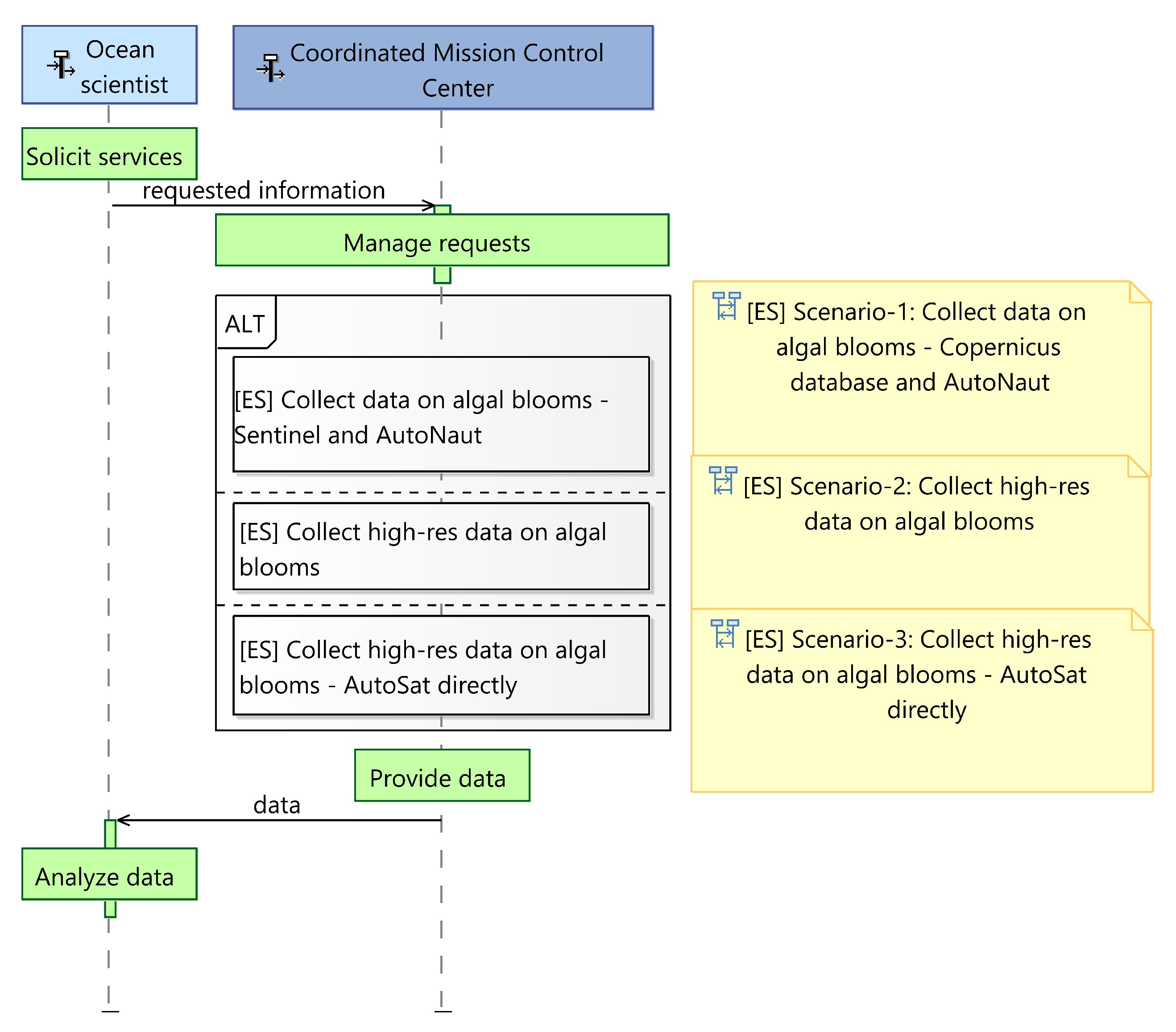
To illustrate how satellite observations can aid in situ observations from unmanned vehicles like the AutoNaut, we explore three scenarios that model the information flow between the assets. Scenario 1 makes use of data from existing EO-sources, while Scenario 2 and 3 rely on a dedicated satellite, represented by HYPSO-1. Furthermore, Scenarios 1 and 2 involve the CMCC as a coordinating entity, whereas Scenario 3 does not, until the final collection and presentation of collected data from both the satellite and the AutoNaut. In Scenarios 2 and 3, HYPSO-1 monitors an area and uses the onboard detection algorithms to determine whether the observation is a natural phenomenon of interest or not. If the retrieved information is classified as such, the satellite forwards directives to the USV. Depending on the scenario and communication mode, the information may be either relayed through an existing ground segment to the CMCC (Scenario 2) or directly to the AutoNaut employing a dedicated communication system (Scenario 3). Despite that direct communication between the satellite and the USV could decrease latency and enable faster in situ response, it comes with challenges related to employing a communication link and the amount of data transmitted. The downlink capabilities onboard the USV might depend on the sea state and the amount of data to be downlinked. Those limitations are negligible if data are first downlinked to ground, post-processed, and then transmitted to the USV in the form of a navigation and data collection plan. This process means that the data forwarded to the AutoNaut by the satellite in the second scenario must be processed operational data including a navigational plan. Once data are received onboard the AutoNaut, the onboard software modifies the goals of its current mission to steer the vehicle towards the desired location and sample the targeted phenomenon.

The three different scenarios, shown in Figure 4, describe how the information flow above can be achieved:

• Scenario 1: the CMCC retrieves data from existing space assets, like Copernicus Sentinels and other EO-satellites, and processes them to detect phenomena that should be investigated in situ. The age of data and the predicted behavior of the phenomena must be included in the processing. In case of detection, the CMCC creates a navigation and sensors usage plan and forwards it to the AutoNaut.
• Scenario 2: a dedicated satellite such as HYPSO-1 monitors a selected AOI and forwards (processed) data to the CMCC. If processed data indicate an ongoing or potential phenomenon of interest, a dedicated mission is built and dispatched to the USV from the CMCC.
• Scenario 3: following an observation from the AOI, a dedicated satellite like HYPSO-1 processes the acquired data onboard and communicates a mission plan directly to the AutoNaut.

Figure 4. Exchange scenario (ES) overview in a lifeline format. The dashed lines indicate the lifeline of the actor, and the solid lines indicate a functional exchange between a source and a target actor. A green box indicates a function, the grey box with [ALT] indicates choices between different ES. The yellow sticky notes are there for linking between diagrams for the user. The figure is modeled using Capella.

Figure 4. Exchange scenario (ES) overview in a lifeline format. The dashed lines indicate the lifeline of the actor, and the solid lines indicate a functional exchange between a source and a target actor. A green box indicates a function, the grey box with [ALT] indicates choices between different ES. The yellow sticky notes are there for linking between diagrams for the user. The figure is modeled using Capella.

Physical events in the oceans are dynamic and constantly changing, and the timelines of information delivery and data latency are important metrics to consider to assess the utility of the system. The lowest data latency and age is achieved through scenarios where onboard processing extracts the important information from the data at an early stage to minimize the data volume to downlink, and hence the time for this data transfer. Scenario 3 has the potential of providing data with virtually no delay between the satellite and the AutoNaut, given some assumptions that are discussed in detail in Section 3.3.3. The three data distribution strategies are explored, compared, and discussed in this paper.

3.3.1. Scenario 1: Satellite Imagery from Existing Infrastructures

In the first scenario, we exploit existing technologies and infrastructures to gather satellite imagery of a selection of AOIs and commanding in situ assets for data collection, as shown in the top path of Figure 5. Specifically, in the spring of 2021, we used the Sentinel database [35] to retrieve processed imagery of Frohavet in mid-Norway and coordinate in situ observation and sampling of coastal areas typically affected by HABs, as discussed in Section 5.

Based on information from the available satellite observations, a user or data processing tool selects an area of interest for the AutoNaut to investigate. The latency of satellite data varies between 3 h and a day, depending on the chosen infrastructure (e.g., Copernicus Sentinels or other). The data spectral and spatial resolution may vary depending on the satellite source used.

This scenario requires a processing pipeline to be available. The data latency will be the sum of the age of satellite data products, the processing and commanding time, and the time needed for data collection and communication to shore from the sampling site. Whereas the time periods for information retrieval using existing infrastructures are usually known, the time required to retrieve to shore data collected in situ depends on several factors as described in Section 3.4.1.

Assumptions for Scenario 1

For Scenario 1, information about the AOI is made available to the AutoNaut based on the EO data processing at the CMCC. This means that the data age is determined by the service level of the data provider, $t_{\mathrm{dataage}}$. Assuming a well-programmed processing pipeline, the time for processing selected data, $t_{\mathrm{processing}}$, will be very short compared with the data age. Furthermore, since this scenario uses existing infrastructure the communication delay, $t_{\mathrm{transmit}}$, can be approximated to zero, since the communication delay through a 4G network or Iridium is negligible if compared to the time scale of the USV navigation capabilities (the distance covered in time) and to the time scale of the observed phenomenon. Hence, the only factor determining the freshness of the data product is the age and availability of EO data. A typical value for this parameter is in the range of 6 to 24 h.

3.3.2. Scenario 2: Dedicated Small Satellite—CMCC—AutoNaut 

Small EO satellites, such as the HYPSO-1 satellite [32], enable more agile and customized operations. The use of such systems enhances the flexibility of the operations, such as the choice of the area to be monitored and use of reconfigurable and adaptive algorithms for compression and processing of the data to be downlinked. The satellite can transmit processed information directly to the CMCC obtained from single or multiple observations. The CMCC is responsible for the definition of the mission plan that should be communicated to the AutoNaut, and hence their communication to the USV, as shown in the middle path of Figure 5.

After making an observation, the satellite must transit from the AOI to the next available ground station until it can transmit data to the CMCC. Similar to the previous scenario, the data product latency is a sum of response time needed for image processing, downlink, ground data processing, and the time relaying the connected data and mission plan to the AutoNaut. The response time of the image processing includes uplinking to the satellite: the time it takes for the target to become observable and be processed onboard.

Assumptions for Scenario 2

For Scenario 2, we use a model simulated in Python utilizing the PyOrbital library for propagating the satellite that is set to observe a selection of AOIs. For each AOI pass, we compute the time until the satellite passes over a ground station and use that as an estimate for when processed data can be delivered to the AutoNaut. The AOIs are defined by their center location to simplify simulations. In this case too, $t_{\mathrm{transmit}}$ can be neglected as the navigational plan data is assumed to be around 100 bytes transmitted over either 4G or Iridium, with a minimum bitrate of 1200 bytes per second for Iridium.

• Since the HYPSO-1 is not launched yet, LUME-1 is used as a representative model. Two Line295Elements (TLEs) are automatically obtained from Celestrack.
• Minimum elevation for optical target observation: 20${}^{\circ }$.
• Minimum elevation for radio communication to ground station: 0${}^{\circ }$.
• Only daylight passes are considered: from 8:00 to 19:00 local time.
• Only onboard processed data are considered to reduce the data size needed for downlinking.
• Ground station locations from the KSAT Lite network are considered. Two simulations are compared, either using one station only or the full network.
• The downlink is based on S-band with 1 Mbps raw data rate.

The impact of Assumption 2 is that the most extreme slant range passes are ignored, so every target is only observable one to three times a day. If omitting Assumption 5, transmitting raw data from the satellite, we would need multiple passes to download the relevant data, which may take hours or days to complete ([32], Table VII), heavily affecting the $t_{\mathrm{dataage}}$. The total time to download data will depend on the length of the observation. Transmitting onboard processed data, such as a target position, will take only seconds under the same conditions. The satellite used for simulations is LUME-1, built for the European project Fire RS from the joint efforts of the University of Porto (Portugal), LAAS-CNRS (France), Universidade de Vigo (Spain), and Alén Space (Spain) [20]. This satellite is in a representative orbit for HYPSO-1, thus simulation results are expected to be similar to what HYPSO-1 will experience.

For some targets, the satellite will see both the target and a ground station simultaneously. The simulations take this into account. Cases where the ground station contact ends at least four minutes after the observation ends to allow for processing time and downlinking are included in the simulation results. For these occurrences, both maximum, minimum, and mean delays are set to zero. This also assumes that booking and scheduling of ground station passes are available so that the satellite can transmit data to the first ground station it passes over.

3.3.3. Scenario 3: Dedicated Small Satellite—AutoNaut 

In the third and last scenario (shown in the bottom path of Figure 5), we envisage a flow of information that makes no use of ground communication infrastructure. After a small satellite, such as the HYPSO-1, makes an observation, data is processed onboard, and instructions and a navigation plan are communicated to the terrestrial assets such as the AutoNaut directly. For example, target detection can be used to create a map showing the most likely locations of a particular spectral signature [36,37]. Either the map can directly inform the path planning or be expressed in a simpler form, such as the most probable location of a bloom. HYPSO-1 plans to use the Adaptive Cosine Estimator for target detection, but constrained energy minimization and the matched filter have also been developed.

The response time and data latency will, in this case, be the sum of the response time for imaging of the selected area, the processing time, the downlinking time, and sampled data transmission to shore. A central topic in this scenario is how to enable the communication infrastructure between the assets. This brings forth challenges with both the physical infrastructure needed (radios and antennas) and network management. This scenario requires that both assets know their location and the location of the other so that communication can be scheduled accordingly.

Assumptions for Scenario 3

We are considering the same target list and simulations as for Scenario 2. In addition, the satellite must reach the AutoNaut in a time-window that both allows onboard data processing and transmission of the navigation plan to the AutoNaut before the satellite is out of view.

The data preparation (onboard processing) time after observations is assumed to be less than one minute. Furthermore, the resulting data volume is assumed small enough to be transmitted over a 10–100 kbps link for less than one minute. The size of the navigational plan and other needed information is assumed to be similar to what is the case today, which is around 100 bytes (see the assumptions for Scenario 2 above). The complete specification of this link is the topic of future work. This requires the AutoNaut to be in the AOI and within satellite coverage for at least one minute after data preparation for downlinking.

3.4. Constraints

Optical sensors operating in the visible range are affected by cloud coverage and, therefore, may have limited detection capabilities. The AutoNaut can be impacted by storms or other weather conditions that both can degrade the data quality and the maneuverability and response time of the AutoNaut. The encompassing system and services must consider CS constraints when defining the SOS operational scenarios and CS requirements.

In this section, we describe the high-level constraints that affect all architectural variants of the proposed system, namely, general constraints that affect the execution of the information flow and that are common to all scenarios.

3.4.1. Wave-Propelled USV Constraints

As most of the marine vehicles whose propulsion is produced by environmental forces, the AutoNaut capabilities depend on the sea state. The velocity of such vehicles is not controllable and therefore, to predict future locations, one must rely on estimates based on present and forecasted sea state. Situational awareness is achieved via onboard sensors that sample physical environmental properties and provide the vehicle control system an estimated present sea state used to adapt the navigation control parameters. Stable course control can also be a challenge whenever the forces exerted by the environment dominate on steering and propulsion mechanisms, preventing the vehicle from following an intended path. The USV’s speed and course are affected by waves direction, height, and frequency and by surface currents and winds. This has a considerable impact on the AutoNaut capability to monitor oceanographic phenomena that occur far from its current location, as the time needed to reach a destination depends on the surrounding environments.

A second major limitation is the onboard energy available. The onboard battery bank is constantly harvesting solar energy produced by deck-mounted solar panels providing the necessary power to sensors and electric steering. Significant power limitations are experienced in winter at high latitudes, where light is not sufficient to recharge the batteries, and the time span of the mission may be reduced. This impacts the possibility of observing specific phenomena as too little energy might prevent the activation of a specific sensor. Moreover, power should not only suffice for sampling specific features but also to allow data transmission to shore (e.g., via Iridium, 4G, or VHF) and navigation control.

Communication is the third constraint that affects operational flexibility. The USV is equipped with three communication links that are used depending on the type and amount of information to be transmitted and the location of the vehicle. Satellite communication (for example, through Iridium) constitutes a reliable link proven to work in most areas of the globe. However, this is costly and limited by the amount of data that can be transmitted. 4G/LTE communication allows transmitting a much larger amount of data even though it is limited by distance to shore. Finally, the VHF radio link, mainly used for telemetry and emergency situations, has a range of tens or hundreds of kilometers depending on the sea state and antennas location.

Data acquired onboard can be stored and transmitted over the mentioned links depending on the type of data and the vehicle location. For example, sea current information for the whole upper water column involves a large amount of data that can be easily transferred over Internet or WiFi but cannot be sent over satellite. It is thus possible to transfer only key information over Iridium or, alternatively, let the USV navigate close to shore within 4G/LTE coverage. For example, key information about a specific water property could be the temporal average of the collected numeric values over predefined time periods.

Based on field experience, it is observed that the USV speed in the ocean fluctuates between 0 and 3 knots, depending on the sea state. Therefore, we can safely assume that the vehicle is capable of traveling on average 30 km per day. Based on the time period of the phenomenon to be observed, the vehicle proximity to the targeted area is a constraint that must be considered during the mission planning phase.

3.4.2. Constraints for Small Satellites

Small satellites can be an agile tool since they are relatively cheap and have a short development time [38]. As satellites such as HYPSO-1 are small, they are influenced by physical constraints leading to system constraints impacting the power/energy availability due to a limited solar array area. Moreover, the size of the satellite may restrict antenna sizes, especially in the VHF and UHF-bands.

The power constraint comes into play in the sense that only a limited part of the Earth can be actively covered at the time because there is limited energy for payload operation and data downlink. A dedicated small satellite has the agility to accept any area of interest defined by the mission operators on short notice. Additionally, in EO missions that generate a large volume of data, both energy for operating the downlink radio leading to a time limitation and data rates are constrained by physical antenna sizes and the availability of ground stations limits the amount of data possible to download every day. The challenge of data volume is mitigated by performing onboard payload processing, thus compressing the data and effectively reducing the data volume by several orders of magnitude. The limitations in coverage, the revisit time over a given area, is a function of the number of satellites in the network and can be mitigated by increasing the number of satellites and orbital planes.

For single satellites, there are some limitations in coverage and agility. The coverage area and accessibility at a given time of day are constrained but well known and defined by the satellite orbit. This can be mitigated by adding more satellites, for example, in different orbital planes. The selection of the AOI must also be done in due time before the satellite passes over a ground station prior to a target pass, so the satellite can prepare for the observation. Initially, operators will determine the AOI by selecting a coordinate for the center of the image, but the development of more sophisticated AOI geometries is a topic of future research. Moreover, adding more ground stations at suitable locations will improve agility.

The integration of autonomous sensor agents into heterogeneous networks together with satellites either as independent sensors or communication relays has been studied in several surveys and proposals [39,40,41,42,43]. Networking principles enabling the network integration encompassing a multitude of agents, by employing standard toolchains and efficient network protocols as well as location-aware smart routing principles are discussed in [44,45,46].

3.4.3. Communication Technologies and Analysis

Scenario 1 will only make use of existing communication infrastructure, both between the EO-satellites and ground systems as well as between the CMCC and the AutoNaut.

For Scenario 2, we can utilize existing radio links between the satellite and the ground stations. Correspondingly, the existing infrastructure for command and control for the AutoNaut can be used. To bind these two constituent systems together, a middleware layer with a messaging protocol must be developed and implemented.

For Scenario 3, the direct communication between the satellite and the AutoNaut must be based on new infrastructure. This is a research topic that should be further explored. It should be mentioned that the recent years have seen an increase in deployments of new satellite-based communication infrastructure, such as IoT-constellations [47] and megaconstellations such as Starlink, OneWeb, or Kupier. However, the use of the megaconstellations is considered not relevant for our scenarios, as their ground terminals will be too big for the AutoNaut. Moreover, the available IoT solutions may still not fill the gap created by low throughput, one-way data traffic, and their method of dealing with multiple access, like providing channel access for users at random time intervals. A limited number of communication channels suitable for each proposed scenario exist.

3.5. Other Architecture Variants

In addition to our suggested architectures discussed as Scenario 1 and Scenario 2, there are options for how the satellite and robotic agents such as the AutoNaut can be interconnected. The satellite could be equipped with equipment creating an Inter-Satellite-Link (ISL) between the small satellite and other space-based infrastructure instead of transmitting its observations to a GS. Possible options include "traditional" satellite phone/Machine-to-Machine communication (M2M) systems such as Iridium, Globalstar, and OrbComm, "traditional" broad-band satellite systems as Inmarsat and Intelsat based on Geostationary Orbit (GEO) satellites, in addition to the new megaconstellations as well as new IoT-satellite constellations. The work behind this paper does not aim to evaluate and compare these options in full, but a brief discussion on the alternatives follows.

Previous studies encompassing mostly Iridium and Globalstar options have shown that such methods will allow for the transmission of a small amount of data, most likely to be adequate to direct the AutoNaut to an area of interest. Rodriguez et al. [48] have summarized several studies in their paper. Several activities are supported by NASA, for example, through their PhoneSat series. In 2021, Riot et al. presented results from an on-orbit experiment which found that an LEO satellite equipped with an Iridium transmitter will be able to deliver low volumes of telemetry within a 30-min delay, for about 90% of the time [49]. This result is comparable to our results for sparse ground stations, see Section 5.2.1.

Making use of networks meant for terrestrial use on-orbit also means that we will have similar constraints for parameters as Doppler shift and maximum usable range, limiting the usable service area from, i.e., the Iridium satellites [49]. In addition, more constraints follow from the combination of orbits, where the inclination has the largest effect. This leads to the case that ISL to low-inclined services (such as OrbComm, Globalstar) is not ideal for polar-orbiting satellites. The same will be the case for crosslinking from LEO to GEO for Inmarsat services, for example.

4. Methods

4.1. Description of Workflow

We followed a simple workflow shown in Figure 6 for the research provided in this paper. In the Modelling and developing operational concept phase, we applied a combination of a whiteboard, virtual meetings and drawings, and discussions to develop the operational concepts and used literature to identify relevant AOIs. These operational concepts were modeled in Capella and iterated on through discussions. In Simulations of scenarios, we set up the scenarios for the simulations with the assumptions given for each scenario in Section 3.3 and Analyzed results to improve the simulations, the scenarios, and to ensure that our assumptions were valid. The AutoNaut Field work experiences were used to validate the results and to provide feedback to the assumptions and simulations.

4.2. Tools Used

In this analysis, we have used the Arcadia method [50] with the open-source Capella software tool (https://www.eclipse.org/capella/, accessed on 11 August 2021) to support the Model-Based Systems Engineering (MBSE) effort and provide an operational and logical architecture of the SOS [51]. The system model enables the representation of the architecture with different viewpoints, such as "exchange scenarios", "context diagrams", and "architecture diagrams". There are also possibilities for integration with domain-specific tools such as System Tool Kit (STK) that can be used to demonstrate the quantitative performances of the proposed SOS.

The simulations have been performed using Python, in particular using the pyorbital library. This library calculates orbital parameters and computes other astronomical parameters from satellites’ TLEs. The TLEs are collected from Celestrak [52].

4.3. Selection of Areas of Interest

The objective of the SOS is to detect but also sample in situ oceanographic phenomena remotely. We choose to observe areas that have historically been affected by phenomena such as HABs. Since HABs can result in the death of farmed fish; the targets selected for our simulations are areas where fish farming is common. The selected targets are popular areas for fish farming and where HABs may occur (see [53] for an overview). These are the Norwegian Atlantic coast near Frøya, the coast of Chile south of Puerto Montt, the coast of Canada near Vancouver Island, the coast of Tasmania in Australia, and Lake Erie [54], a fresh-water lake in the US where HABs are common. These locations and the considered ground stations are shown in Figure 7.

4.4. Communication Delay Estimation

One of the key metrics for evaluating the performance of the data flow and utility of the SOS is the data delay, meaning the time from observation to the data is available for the AutoNaut. In this case, the "data" is the navigational plan and all information needed for the AutoNaut to perform its operations. The time for returning samples and analysis from the AutoNaut will be the same for all three scenarios, so this duration is omitted in further discussion.

Equation (1) shows how we estimate the total delay in time ($t_{\mathrm{total}}$) between when an observation of an oceanographic event of an AOI is made to when the AutoNaut is notified and commanded to investigate this event in situ. $t_{\mathrm{dataage}}$ is the age of the observation data until it is processed either on ground or in orbit, $t_{\mathrm{processing}}$ is the time spent for data processing, and $t_{\mathrm{transmit}}$ is the time it takes to transmit a set of commands to the AutoNaut.

For Scenarios 1 and 2, $t_{\mathrm{transmit}}$ is assumed to be equal since both cases rely on using the same communication infrastructure from the CMCC to the AutoNaut. The value for this delay is in the range of hundreds of milliseconds to a few seconds, based upon 4G or Iridium. The range for the processing time, $t_{\mathrm{processing}}$, is from seconds to a few minutes. The value for $t_{\mathrm{transmit}}$ is assumed to be less than two minutes. This is based upon the assumptions for the communication links listed above and the size of the navigational plan, which is about 100 bytes.

$$t_{\mathrm{total}}=t_{\mathrm{dataage}}+t_{\mathrm{processing}}+t_{\mathrm{transmit}}$$

(1)

4.5. Simulations

Based on the above assumptions, a short Python program was implemented to generate a set of times for when the satellite can observe the targets and deliver the observational data either to the CMCC through a ground infrastructure (Scenario 2) or directly to the AutoNaut (Scenario 3). For Scenario 2, two different simulations were performed, one with only one ground station and one with all the ground stations of the KSAT Lite network available.

The function called get_next_passes from pyOrbital library was used to estimate when the satellite was over the ground stations and the target areas. The main parameters specified for the simulations are: start date (exact date and time to start the simulations), number of hours to simulate, coordinates of observation location (longitude and latitude) altitude above sea level and minimum elevation for contact between location and satellite (minimum elevation for a pass). The simulation start date was set to 2021-06-09 16:00 and the time to simulate for a week. First, all possible passes over the targets and the ground stations are computed. The passes over the targets are limited to those during daylight (between 8:00 and 19:00 local time). For each target pass, the delay is estimated as the difference between the start time of each ground station pass and the end time of the target pass. When the difference between the end of a ground station pass and the end of a target pass is longer than a minimum communication window, the delay is saved. The ground station whose pass offers the minimum delay after an observation of a target is considered the first ground station used. The maximum delay and the mean delay are calculated for each target pass. The simulations are performed both for a sparse ground station network (just one ground station) and dense ground station network (where six ground stations are used).

5. Results

In this section, the different scenarios and their utility are explored.

5.1. Scenario 1: Coordinated Observation of HABs

The information flow described in Scenario 1 was tested in the field in Spring 2021, in the context of HAB coordinated observation involving both aerial and terrestrial platforms. This experiment involved several manned and unmanned robotic assets for a duration of over one month and the objective of the field campaign was to study the algal bloom at different space and time scales, from satellite observations of the whole Frohavet region down to the underwater sampling of the epipelagic (upper) water column. In particular, satellite-based imagery was acquired from Sentinel-3, Terra and Aqua (MODIS data) and PRISMA (https://www.asi.it/en/earth-science/prisma/, accessed on 11 August 2021) when available. The imagery, see Figure 8, recorded on 14 March was used to monitor the growth of the algal bloom in the operational area and assist with high-level mission planning and coordination of the involved robotic platforms gathering in situ measurements.

Among the assets, the AutoNaut was the first deployed, and it provided the overall mission insight into how algae grew and multiplied in the period leading up to the bloom. The wave-propelled AutoNaut was at sea for a total of 24 days, collecting and transmitting data continuously over 4G and Iridium communication. In addition to providing additional long-term insight into the algal bloom dynamics itself, the wave-propelled USV collected data to be used to validate hyperspectral cameras carried by the involved UAV and airplane. Figure 8 and Figure 9 also show the track covered by the AutoNaut in Frohavet on March 14th and the surface chlorophyll-a data collected in situ. It can be observed that the surface chlorophyll-a measurements performed by AutoNaut validate the Sentinel-3 observations in the same area.

5.2. Scenario 2: Satellite—CMCC—AutoNaut 

The delay from an observation to the CMCC was simulated for two different sub-cases; one with only one ground station available. Svalbard is selected as it is seen by all revolutions by a polar orbiting satellite. This is called a sparse ground station distribution. The second run where all the ground stations of KSAT Lite network were available is called dense ground station coverage. This delay will give an estimate for the $t_{\mathrm{dataage}}$ for this scenario. The simulation is run for one week starting from 9 June 2021. The satellite orbit is based on TLEs for the LUME-1 satellite, received from Celestrack. LUME-1 moves south-to-north over Western Europe during daylight hours. In both cases it is assumed that the AutoNaut is within 30 km of the center of the AOI, as this is the range the AutoNaut may navigate during the day.

5.2.1. Sparse Ground Station Coverage

For Scenario 2, the satellite will acquire and process the data, before it needs to reach a GS to forward the data to the CMCC for final processing and forwarding to the AutoNaut.

With $t_{\mathrm{transmit}}$ in this case being similar to Scenario 1, $t_{\mathrm{processing}}$ is similar to Scenario 3, it is again $t_{\mathrm{dataage}}$ that will be the driving factor for $t_{\mathrm{total}}$.

From the column named Delay stats for single GS in

Table 1. Statistics for dense and sparse ground station coverage (mm:ss) for one week, showing the delay from end of an observation to the first available ground station.

	Delay Stats for Single GS			Delay Stats for GS Network
	min	max	mean	min	max	mean
Lake Erie (USA)	06:38	07:59	06:59	01:53	03:34	02:31
Western coast of Chile	29:58	31:08	31:08	05:56	10:40	07:42
Tasmania (Australia)	27:46	28:28	28:09	12:25	15:01	12:22
Vancouver (Canada)	05:40	06:59	06:08	00:00	00:00	00:00
Frøya (Norway)	00:00	00:00	00:00	00:00	00:00	00:00

, we can see that for a single ground station, the delay (meaning the duration after an observation until the satellite can reach the ground station at Svalbard) varies from about 0 minutes for the Frøya target to about a half hour for Chile and Tasmania targets. This duration/delay corresponds to the value for the parameter $t_{\mathrm{dataage}}$ in Equation (1).

5.2.2. Dense Ground Station Coverage

Column Delay stats for GS network in Table 1 shows the results for the minimum time after an observation until the satellite reaches a ground station, given the availability of the full KSAT Lite ground station network. From the simulations, we see that the mean time to reach a ground station varies between 0 and less than 13 min, depending on the target location. For all targets with a delay larger than 0, there is a reduction compared to the sparse ground station setup. Tasmania and Chile targets have their mean delays more than halved.

The number of instances for when a ground station was the closest after a target observation is shown in

Table 2. Count of first ground station used after each target for the simulated period.

	Inuvik	Panama	Tokyo	Fairbanks	Vardø	Tromsø
Lake Erie	7	0	0	0	0	0
Chile	0	8	0	0	0	0
Tasmania	0	0	7	0	0	0
Vancouver	3	0	0	6	0	0
Frøya	0	0	0	0	4	10

. Such mapping can also be used to derive and plan which stations should be utilized and which stations can be removed to reduce cost, for example. Since the satellite is in an Sun-Syncronious Orbit (SSO) type orbit, where we only are interested in daylight passes, the same ground stations will be utilized every time. From the table, we observe that maximum two stations are needed for each target. In this particular case, we observe that Inuvik is the station that may collect data from the highest number of targets.

5.3. Scenario 3: Direct Communication between Satellite and USV

For Scenario 3, the observation time, including onboard processing, represents the value for $t_{\mathrm{dataage}}$ and is in the range of one to two minutes [32].

The short onboard processing time, $t_{\mathrm{processing}}$, (about one minute), allows for transmission of a short message to the AutoNaut immediately after an observation is made, given that the AutoNaut is in the vicinity of the AOI. The observation time is set to 2 min for all occasions, starting when the satellite is at Acquisition of Signal (AOS). This is following the operational concept of the HYPSO-1-mission [32] plus a one-minute margin. This scenario is depicted in

Table 3. Simulations of target observations and communication windows to the AutoNaut.

	Target	Target	Target Max	Target	Autonaut	Avail. Time
Target	AOS	LOS	Duration	obs. End	LOS	for Comms
Lake Erie	15:16:35	15:21:15	00:04:40	15:18:35	15:24:34	00:05:59
Chile	13:20:37	13:23:01	00:02:24	13:22:37	13:27:14	00:04:37
Chile	14:53:50	14:56:43	00:02:53	14:55:50	15:00:42	00:04:52
Tasmania	00:44:48	00:48:53	00:04:05	00:46:48	00:52:29	00:05:41
Vancouver	18:50:53	18:55:16	00:04:23	18:52:53	18:58:42	00:05:49
Frøya	07:32:35	07:34:46	00:02:11	07:34:35	07:38:54	00:04:19
Frøya	09:04:29	09:09:19	00:04:50	09:06:29	09:12:35	00:06:06

. In this case, the value for $t_{\mathrm{transmit}}$ will be in the order of seconds for transmission of navigation coordinates and instructions. The total delay, $t_{\mathrm{total}}$, is then within two to three minutes, so near real-time operation is possible.

Table 3 shows all daylight passes for the 16 April 2021, with times in Universal Time595Coordinated Orbit (UTC). The columns indicate when the target is visible which is the time between Target AOS and Target LOS. This gives a total possible observation time. Furthermore, 2 min was chosen as the actual observation time, leaving a given duration available for processing and communication between the observation end and the AOS-event for the AutoNaut.

6. Discussion

We consider the three different architecture variants as introduced, and through simulations and analysis, we present the main findings that were focused on satisfying a HAB use case. The architecture variants are generic but are exemplified and evaluated through simulations employing properties of the HYPSO-1 satellite and the AutoNaut as example implementations. The main advantage of the proposed solution is that the multi-asset and multi-sensor approach can enable near real-time coordinated oceanographic observations of HABs, which are challenging to detect and classify.

Main results:

• In Scenario 1, the $t_{\mathrm{total}}$ is expected to be 3–24 h, based on the publishing time for traditional EO-data. This limits the operational real-time use of this type of data. In addition, the AOIs cannot be selected by the end-user.
• For Scenario 2, the mean value of $t_{\mathrm{total}}$ is less than 16 min for a dense ground stations network and less than 30 min for all selected targets if only a single ground station is used.
• For Scenario 3, the $t_{\mathrm{total}}$ is estimated to be on the order of 1–3 min, given the assumptions listed.

Even without direct contact between a satellite and a USV, it is possible to transmit fresh EO-data from a remote sensing satellite to an in situ vessel as the AutoNaut within 30 min for most cases. The use of onboard processing and existing infrastructure will make this scenario possible with little cost and effort. Depending on resources and delay requirements, one or more GSs from a commercial ground station supplier can be used to enable this. Which GS to use can be decided on based on simulations, as shown in this paper. A CMCC must be in place, integrating the communication satellite and the USV(s) through a common middleware layer.

6.1. Scenario Evaluation

The three scenarios are analyzed and discussed in the following.

6.1.1. Scenario 1

In Scenario 1, no efforts are needed to ensure periodical delivery of the required imagery. Moreover, several EO data sources are accessible for no cost. Despite these advantages, the chosen services and infrastructures are not configurable, so the end-user cannot select the AOI the EO-satellites will observe and have instead to rely on historical data and a "best-effort" revisit time. Moreover, the age of the observational data is arbitrary and near "real-time" operation with a data age requirement of less than 6–24 h cannot be supported. This would affect the in situ observation and sampling of targeted phenomena which are commonly defined in a limited time frame.

A processing pipeline for selecting/filtering and processing of the EO data must be created and can be based on existing frameworks and technologies. In addition, a middleware layer integrating the processing pipeline and the commanding software for the AutoNaut must be developed, but no other infrastructure will have to be developed. An example of this scenario is provided in Section 5.1, where satellite imagery from existing infrastructure is used to command marine and aerial assets with the purpose of observing a HAB.

6.1.2. Scenario 2

In Scenario 2, we estimate the time from when a dedicated satellite makes an observation until this data can be used for instructions and navigation plans for the AutoNaut. Similar to Scenario 1, this scenario also relies on existing infrastructure, except for the need of an CMCC with a processing pipeline and middleware layer able to integrate messages between the satellite and the AutoNaut. A dedicated satellite that can be commanded to observe selected AOIs may deliver information to the AutoNaut 30 min later, even if only one ground station is used (this time will vary depending on the target locations.) If a full GS network is used, this time can be further reduced, down to about 15 min. As shown, targets within Arctic/sub-Arctic areas are close to existing GSs; thus the time between an observation and a downlink pass may be close to zero.

Even with using only one ground station, we see that for the case of Frøya (Norway) the satellite will see both the target area (Frøya) and the ground station (Svalbard) at the same time for part of the observation pass. This means that the data can be downloaded immediately after processing. For the simulation, useful communication passes must end at least 4 min after the observation ended. This in order to have time to do both processing (limited to one minute, similar to Scenario 3) and perform downlinking in a reasonable time. All passes in this simulation leave more than 5 min for downlinking.

When making the full GS-network available for the simulation, the simulator will choose the closest usable ground station in each case. For example, we see that the assumed best station (Svalbard, as it is seen from all satellite orbital passes) is then not used since other stations can pick up the signal from the satellite earlier. In addition to utilizing existing infrastructure, the main advantage of Scenario 2 is that satellite data can be requested and retrieved on-demand. Onboard data processing will reduce the size of data to be transmitted to ground, thus reducing energy for operation of the radio system as well as the time to download the data. Selecting the number and locations of GSs will impact the response time of the system and possibly also influence the cost of ground station lease, depending on the commercial model of the ground station provider (if accessing more than one GS costs more than one, or if it is only the time of access that determines the cost).

6.1.3. Scenario 3

The main advantage of Scenario 3 is that, depending on the communication delays between the satellite and the USV, the closed-loop from space observation to in situ sampling and data analysis on shore observation of an oceanographic phenomenon can be achieved with lower data latency and time responses compared to Scenarios 1 and 2. Despite such benefits, this implementation comes with some limitations concerning the data processing capabilities onboard both assets, the need of resilient algorithms for human supervision/intervention, and a robust communication link between the assets. The possibility of adding onshore processing and data from other sources in Scenario 2, as the CMCC can make use of larger computational capabilities to run complex metocean models on the base of satellite observations, may outweigh the gain of a faster response in Scenario 3. This could help to optimize the missions commanded to terrestrial assets and thus the quality of data retrieved to shore.

7. Conclusions

Our analysis indicates that an architecture like the SOS presented in this paper can be used for tailored and adaptive observation systems, adapted to their specific target areas. The commonality of a generic architecture consisting of satellite(s), a CMCC, and in situ agents can be utilized to observe a great variety of oceanographic properties and geographic regions. The specific satellite and in situ platform and instrument can be adapted to season or other properties.

The specific properties of the different architecture variants can be exploited to match different purposes, and they come with different costs for implementation and resources for realization. Scenario 1 is available today, as demonstrated in our field experiment. The real-time constraints of this scenario as well as the limitation in an active selection of AOIs motivates the exploration and development of Scenarios 2 and 3. Like Scenario 1, Scenario 2 is available with existing technology or technology available in the near future. Scenario 2 can provide fresh data, both for a dense and sparse ground station topology. The cost of using more ground stations has to be traded against the gain of getting data up to 1 to 20 min earlier. Optimal ground stations can be chosen based on target selection and similar simulations, as shown in this paper. Even though the difference in data delivery times between those scenarios is on the order of 30 minutes in favor of Scenario 3, the architecture variant of Scenario 3 represents the possibility of tighter integration between sensor agents, without the need of inclusion of a CMCC.