
BFAST Lite: A Lightweight Break Detection Method for Time Series Analysis


Laboratory of Geo-Information Science and Remote Sensing, Wageningen University & Research, Droevendaalsesteg 3, 6708 PB Wageningen, The Netherlands
*
Author to whom correspondence should be addressed.
Remote Sens. 2021, 13(16), 3308; https://0-doi-org.brum.beds.ac.uk/10.3390/rs13163308
Submission received: 26 July 2021
/
Revised: 17 August 2021
/
Accepted: 19 August 2021
/
Published: 21 August 2021
(This article belongs to the Special Issue Time Series Analysis in Remote Sensing: Algorithm Development and Applications)
Abstract
:BFAST Lite is a newly proposed unsupervised time series change detection algorithm that is derived from the original BFAST (Breaks for Additive Season and Trend) algorithm, focusing on improvements to speed and flexibility. The goal of the BFAST Lite algorithm is to aid the upscaling of BFAST for global land cover change detection. In this paper, we introduce and describe the algorithm and then compare its accuracy, speed and features with other algorithms in the BFAST family: BFAST and BFAST Monitor. We tested the three algorithms on an eleven-year-long time series of MODIS imagery, using a global reference dataset with over 30,000 point locations of land cover change to validate the results. We set the parameters of all algorithms to comparable values and analysed the algorithm accuracy over a range of time series ordered by the certainty of that the input time series has at least one abrupt break. To compare the algorithm accuracy, we analysed the time difference between the detected breaks and the reference data to obtain a confusion matrix and derived statistics from it. Lastly, we compared the processing speed of the algorithms using both the original R code as well as an optimised C++ implementation for each algorithm. The results showed that BFAST Lite has similar accuracy to BFAST but is significantly faster, more flexible and can handle missing values. Its ability to use alternative information criteria to select the number of breaks resulted in the best balance between the user’s and producer’s accuracy of detected changes of all the tested algorithms. Therefore, BFAST Lite is a useful addition to the BFAST family of unsupervised time series break detection algorithms, which can be used as an aid in narrowing down areas with changes for updating land cover maps, detecting disturbances or estimating magnitudes and rates of change over large areas.
1. Introduction
The lengthening of remote sensing satellite data archives is opening up new opportunities for the field of Earth Observation. It is now possible to monitor changes of the Earth’s surface better than ever before, as long time series facilitate data-driven analysis methods. A long time series provides information about the usual variability over time within a monitored area, providing an opportunity to detect deviations from the norm in near real-time. It also gives the opportunity for change detection algorithms to identify historical changes with more confidence.
These developments have resulted in an increase in the number of algorithms for change detection in satellite imagery time series. Algorithms such as LandTrendr [1], Breaks For Additive Season and Trend (BFAST) [2] and BFAST Monitor [3], Continuous Change Detection and Classification (CCDC) [4], Exponentially Weighted Moving Average Change Detection (EWMACD) [5], Time-Series Classification approach based on Change Detection (TSCCD) [6] as well as Jumps Upon Spectrum and Trend (JUST) [7] have been introduced with the aim of aiding the efforts of land cover change detection.
Some of these algorithms have been well established and widely used, e.g., the BFAST family, LandTrendr and CCDC. Recent developments on these algorithms include improvements to upscaling and ease of use, such as implementing them on big data platforms such as Google Earth Engine [8,9]. In contrast, many other change detection algorithms are at the proof-of-concept stage. Such proof-of-concept algorithms are not yet accessible as widely, as they either do not have a publicly available, efficient and easy-to-use implementation or have not yet been proven at a large scale and using real remote sensing data. As a result, it is complicated for end-users to adopt proof-of-concept algorithms, whereas optimising them and making them user-friendly requires considerable software development effort. Thus, focusing development efforts on improving algorithms that are well-established already is beneficial for rapid dissemination of the improvements to a wide user audience.
The BFAST family of algorithms has proven to be a particularly popular choice for change detection in satellite imagery time series. The BFAST family includes the namesake BFAST [2], focused on detecting multiple breaks in a time series; BFAST Monitor [3], focused on detecting a single break at the end of the time series for near-real time change monitoring; and BFAST01 [10], focused on characterising the trajectory of the time series around its largest break. These algorithms have been successfully used in many studies, ranging from semi-arid regions of Australia [11] to various ecozones in Canada [12], forest disturbance in the Colombian Andes [13] and turning point characterisation in sub-Saharan drylands [14]. The bfast package has even become a basis for new change detection packages that implement change detection frameworks, such as TSS.RESTREND [15] and STEF [16].
However, there are several limitations to the original BFAST algorithm that affects its uptake by the users. The original BFAST algorithm, as proposed by Verbesselt et al. [2] and implemented in the bfast R package, consists of several stages, of which one requires decomposition of the input time series into trend and season components. This decomposition step, in turn, requires a complete regular time series with no missing data, which is rare when using optical satellite imagery due to cloud cover. In addition, BFAST uses an iterative approach for convergence of change, in both the seasonal and trend components. This approach takes a significant amount of processing time.
To overcome these limitations of the original BFAST algorithm, in this paper, we introduce a new unsupervised change detection algorithm, called BFAST Lite. BFAST Lite aims to improve upon the original BFAST in terms of speed and flexibility. This is achieved by omitting the decomposition of the time series entirely, using a multivariate piecewise linear regression to do model fitting in a single step. Therefore, BFAST Lite can handle missing data in the time series without any interpolation. It is also much faster, as it omits both the computationally demanding decomposition step and the iterative model refitting approach. Speed improvement is important for upscaling break detection to larger areas, especially for a global scale, whereas better handling of missing data is particularly important at locations where cloud cover is common. In addition, BFAST Lite has more tunable parameters, which enables the calibration of the algorithm for particular locations or using machine learning algorithms to combine multiple BFAST Lite models for automatically increasing change detection accuracy.
BFAST Lite is easily accessible for users as a function in the version 1.6 of the bfast R package. BFAST Lite is particularly simple to use for current users of the bfast package, who are already familiar with other BFAST algorithms provided by the package.
The objective of this paper is to detail the implementation of the BFAST Lite algorithm and compare it with the existing algorithms in the BFAST family. In this paper, we first described the implementation of the BFAST Lite algorithm, the differences from the BFAST algorithm and its tunable parameters. We then compared BFAST Lite to two existing algorithms in the BFAST family, BFAST and BFAST Monitor, in terms of break detection accuracy and processing time. For this purpose, we used a global land cover change reference dataset created as part of the Copernicus Global Land Services Land Cover 100 m (CGLS-LC100) project, which includes information about all land cover transition types.
2. Data and Methods
2.1. The BFAST Lite Algorithm
The BFAST Lite algorithm is an adaptation of the BFAST algorithm, as described in Verbesselt et al. [2]. As a brief overview of the original algorithm, BFAST is an unsupervised time series change detection algorithm specialised in detecting multiple breakpoints within a multi-year time series. It works by first decomposing an input vegetation index time series into trend (), seasonal () and error () components using Seasonal decomposition of Time series by Loess (STL) [17]. Next, the trend and season components are tested for at least one significant break in the whole time series using an ordinary least squares residual moving sum (OLS-MOSUM) statistical test. If there is significant evidence () of a break in either the trend or season component, then a process of fitting a univariate piecewise linear regression to determine the locations of the breakpoints (as defined by Bai and Perron [18]) is carried out for each of the components. The decomposition and fitting process is repeated iteratively until convergence is reached.
In contrast, BFAST Lite involves only two steps. The first is the generation of regressors for the piecewise linear regression. This is done by curve fitting on the input time series: the trend is modelled by a monotonous line, harmonics by a sine and a cosine component for each harmonic order [19] and seasonality by seasonal dummies [20]. There is also an option to include autoregressive (lag) terms, as well as to manually include external regressors, for example, spatial neighbourhood features, as presented by Dutrieux et al. [21]. This step is highly user-configurable. The user chooses which of these regressors to include in the model to be fit on the time series. In addition, the harmonic component order and the number of seasonal dummies per year are both user-configurable parameters.
The second step is breakpoint estimation following the approach of Bai and Perron [18], implemented by Zeileis et al. [22] and equivalent to the last step within an iteration in the original BFAST algorithm. To estimate breakpoint timing, this approach creates a number of piecewise linear regressions, where each segment has its own estimates for the regressor coefficients. The break timing is determined by minimising the residual sum of squares (RSS) of the piecewise model, repeated for each possible number of breaks in the time series. The optimal number of breaks is then selected using an information criterion. BFAST prescribes the use of the Bayesian Information Criterion (BIC), whereas BFAST Lite defaults to a more conservative metric developed specifically for piecewise linear regression by Liu et al. [23] (LWZ). While the information criterion of Liu, Wu and Zidek (LWZ) is the default, BFAST Lite allows the user to choose between LWZ, BIC, Akaike’s Information Criterion (AIC) and minimum RSS. Support for custom user-defined information criteria is planned for future releases.
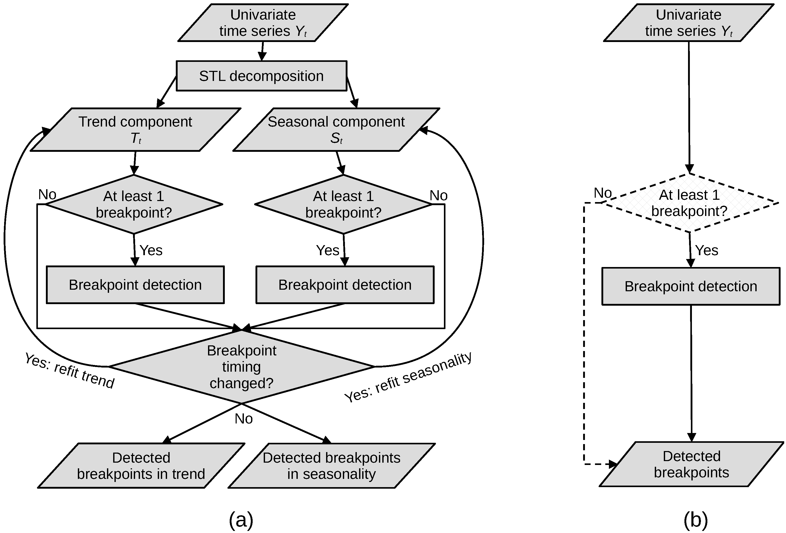
The difference between the BFAST and BFAST Lite algorithms is depicted in a simplified flowchart in Figure 1. The design of BFAST Lite leads to several differences from the original BFAST algorithm. First, BFAST Lite implements the approach of Shao and Campbell [24], in which the time series season and trend components are modelled in a multivariate piecewise linear regression instead of using STL for decomposing the time series as in the original BFAST. This is advantageous for two reasons: (1) it alleviates the need of an iterative decomposition step, making the algorithm faster; (2) it negates the issue of handling missing data in the time series because a (piecewise) linear regression does not require regular interval time series. The drawback of BFAST Lite compared to BFAST is that the detected breaks can no longer be separated into seasonal and trend breaks.
Another difference is that, unlike BFAST, BFAST Lite does not prescribe the use of a structural change test (e.g., OLS-MOSUM) for detecting whether at least one breakpoint is present. It is left as an option to the user and not enabled by default. On one hand, a preliminary structural change test can be beneficial to further reduce processing time by skipping time series that do not have significant breaks. On the other hand, such a test may also cause an increase in omission error, as it is very fast but not as accurate in determining breaks as the much more sophisticated BFAST algorithms. If the structural change test produces a false negative, none of the real breaks in the time series will be detected. Therefore, BFAST Lite gives users the freedom to not use a test or to select any test (not limited to OLS-MOSUM) from the strucchangeRcpp package.
Lastly, BFAST Lite output includes new, more robust statistics to indicate the magnitude of each break. BFAST provides the magnitude based on only the difference between the modelled values at the time step immediately prior to a detected break and a time step immediately following the detected break. This may lead to spurious magnitude values, as the difference between the two time steps may be influenced by a different phase in the modelled seasonality, causing either an exaggerated or a modulated magnitude value depending on the alignment of the seasonality between the adjacent time series segments. In contrast, BFAST Lite provides two more robust metrics of magnitude: the root mean squared deviation and the mean absolute deviation between the model predictions of the adjacent segments over the time span of one year before and after the detected break. The mean deviation is also provided and gives an indication of the change direction, that is, whether the index values increase or decrease after the break.
The BFAST Lite algorithm has been published as a function (bfast::bfastlite()) implemented in R in the free and open-source bfast package, starting from version 1.6.0, available on CRAN. The source code can be found on GitHub, at https://github.com/bfast2/bfast [25], accessed on 20 August 2021. The package is now maintained by volunteers, with GitHub infrastructure facilitating more rapid update cycles, code review and continuous integration. Users are encouraged to submit bug reports and ideas for improvement via GitHub.
2.2. Testing the Performance of BFAST Lite
2.2.1. Compared Algorithms
We compared the performance of BFAST Lite in both break detection accuracy as well as run time with two other well known BFAST algorithms: BFAST and BFAST Monitor. For simplicity, all parameter values for the three algorithms were left at their default values where applicable. The BFAST Lite default values were set to correspond to the default values of BFAST. BFAST has few customisable parameters, most parameters are preset and not adjustable; thus, for comparability, we adjusted BFAST Lite parameters to match those of BFAST. BFAST prescribes the use of BIC for selecting the optimal number of breaks; however, in this study, we tested BFAST Lite using both criteria: BIC and the newly implemented LWZ. For both BFAST and BFAST Lite, the minimal segment size h was set to the number of observations per year. The models were fitted using both a trend component and a seasonal component. The seasonal component was represented by three orders of harmonics, that is, sine and cosine waves at the frequency of one year, half a year and one-third of a year. BFAST mandates the harmonic orders to be set to these three orders, whereas BFAST Lite allows the user to choose any number of orders. We chose to use three orders with BFAST Lite as well for comparability with BFAST. See Appendix A for a detailed list of parameter differences between the two algorithms.
The BFAST algorithm cannot handle missing values by default; thus, we tested two solutions. One is to impute the missing values by linear interpolation between the two neighbouring values in time. This has been the most common approach to handling missing values in research so far, owing to its simplicity [12,26]. The second is to use a more advanced imputation method implemented by Hafen [27] in the package stlplus, which reconstructs the missing values by taking also the values in the same season within neighbouring years into account. This option has also been newly implemented in the bfast package for the original BFAST function, starting from version 1.6.0. This imputation approach results in a smoother time series without interruptions in seasonality, compared to the linear interpolation approach.
The BFAST Monitor algorithm [3] uses a very different approach to break detection compared to BFAST and BFAST Lite. It is designed for detecting a single break at the end of a time series. BFAST Monitor works by splitting the time series into a stable history period that contains usual variability without breaks and a monitoring period, within which the algorithm attempts to detect a break. A linear model is fit on the stable history period extrapolated over the monitoring period, and the predictions are compared with actual data in the monitoring period. While a direct comparison between BFAST (Lite) and BFAST Monitor is difficult due to these differences, BFAST Monitor has been successfully used in the past to detect multiple breaks. This was achieved by running BFAST Monitor iteratively with successive monitoring periods, e.g., yearly [28].
In this study, BFAST Monitor was run yearly over the three years for which we had reference data. The model values were left at their defaults when possible. The linear regression components (regressors) and harmonic order were set to match the other models. When testing the run time of the algorithms, we considered the sum of all three runs of BFAST Monitor to represent the run time of the algorithm.
With the release of the bfast version 1.6.0, a new backend engine written in C++ was introduced. It replaces the previous R engine by default with the option to switch back to the R engine if desired by the user. This change was done to substantially decrease the time needed to run all of the BFAST family algorithms.
The run time of the algorithms was measured using the microbenchmark package [29]. It runs all of the algorithms interleaved to avoid any effect of random busy periods of computer activity on the benchmark results. It also repeats the benchmark multiple times to ensure robust results.
For the purpose of time benchmarking, we selected a smaller subset from the reference data (see Section 2.2.3) using principal component analysis to retain a diverse dataset. We further filtered out points with too many missing values that prevented any of the algorithms from running successfully, resulting in a set of 288 points. Each algorithm was run five times on this dataset, and the time needed to run was compared between the algorithms. We included both interpolation options for BFAST and tested both the iterative approach, as originally proposed by Verbesselt et al. [2], and running the algorithm for a single iteration only. The benchmark was run on a virtual machine on the Terrascope cluster, running on an Intel Xeon (Skylake) processor with 4 cores and 8 gigabytes of memory. The benchmark was run sequentially on a single thread.
2.2.2. Satellite Data
BFAST algorithms are flexible with regards to the input time series that is required for carrying out break detection within it. For the best results, a vegetation index time series derived from a long archive (more than five years) of satellite imagery should be used. The input time series should have as dense observations as possible (at least monthly) to better model the seasonality, although yearly observations can also be handled if no seasonality is modelled. The observations should also be cloud-free by performing temporal outlier removal if necessary. This way, changes in vegetation can be detected with less uncertainty thanks to the length of the time series and with higher temporal accuracy thanks to dense observations. The time series may be irregular, although the original BFAST algorithm specifically requires a gap-filled time series with no missing values.
In this study, as input to the algorithms, a 16-day composite time series of MODIS surface reflectance at 250 m (MOD09Q1 v006) was used. The time series covered the period from 2009 until 2020. The imagery was preprocessed to remove pixels marked as clouds, cloud shadows, ocean, snow and invalid/missing using the included product state quality assurance layer. Next, the NIRv vegetation index [30] was calculated from the surface reflectance, using the formula:
In this formula, is surface reflectance at certain wavelengths: at 860 nm and at 645 nm. NIRv was chosen over other indices due to a lower saturation effect and closer link to gross primary productivity [30] and the fact that it does not require any coarser resolution bands than those provided by the MOD09Q1 product. Lastly, the data were resampled using bilinear interpolation to align exactly with the 300 by 300 m grid that the reference samples used. The time series of the pixels at reference data locations were used for all subsequent analysis.
2.2.3. Reference Data and Validation
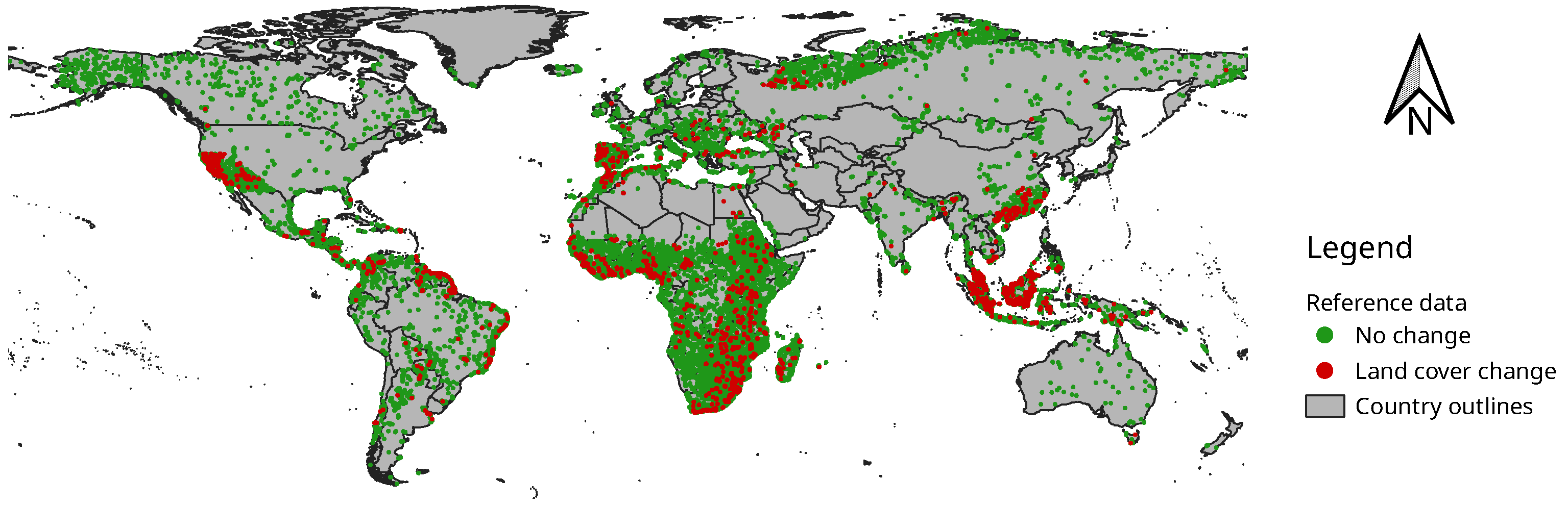
To measure the accuracy of break detection, we used the land cover change reference data that were collected by the International Institute for Applied Systems Analysis (IIASA) as part of the CGLS-LC100 project [31]. The reference dataset is visualised in Figure 2. It consists of 33,881 300 by 300 m sample sites worldwide, of which there are 2594 sites with land cover change (7.7%). Experts at IIASA collected the land cover change reference data by visual interpretation of very high-resolution and Sentinel-2 imagery of the years 2015–2018, assisted by time series of Sentinel-2, MODIS and PROBA-V vegetation indices. The reference data cover a broad range of land cover change, e.g., flooding, deforestation, agricultural expansion, land abandonment, etc.
An important point to consider is that while land cover change and breakpoints in time series are correlated, they are distinct from one another. For instance, forest regrowth is a gradual change process in terms of vegetation index time series and involves no breaks. In contrast, in terms of land cover, forest regrowth involves three changes: bare soil to grass, grass to shrubs and shrubs to trees. Conversely, a break in time series may not result in land cover change, e.g., a burnt grassland stays a grassland next year, even though its vegetation index experiences an abrupt change between the years. Therefore, we used the p-values of the OLS-MOSUM structural change test, the same test that BFAST employs to filter out time series with no change prior to running, to assign probabilities of change to every time series. We then analysed the accuracy of each algorithm, binning the results based on the probability of there being at least one break in the time series, as reported by the OLS-MOSUM test. That way we can be more confident at the higher and lower ends of the probability gradient that breakpoints (or lack thereof) in these time series correspond to land cover change (or lack thereof).
Calculating the accuracy of detected changes is challenging, and defining methods and statistics for this purpose is still an active field of research. This is due to the fact that it is highly unlikely that an algorithm could predict the timing of a break in perfect agreement with the assessment of an expert interpreter. The issue is worse in cloudy areas, where fine spatial resolution observations available to the interpreter differ in frequency from the coarse spatial but high temporal resolution observations input to the algorithm. For instance, an interpreter may only have one image per season, which only allows pinpointing the time of break at a half-year precision. Thus, even though our reference data included an indication of the timing of the change within the year, it was not always highly accurate due to the aforementioned reason, and if the time of change could not be determined, it would default to January 1st. Another issue is data imbalance, as the majority of the reference data indicates no change since land cover change is a relatively rare phenomenon.
For the purpose of assessing how well time series break predictions match the reference data, we developed a distance-in-time approach similar to that proposed by Zhou and Del Valle [32]. We treated each reference and predicted break as an event and then determined whether it was a true positive, false positive, false negative or true negative. If both the predicted and reference breaks overlap within a tolerance distance, it is considered a true positive; if a predicted break does not overlap with a reference break, it is considered a false positive; and if a reference break does not overlap a predicted break, it is considered a false negative. We chose ±1 year as a tolerance threshold, as per previous studies [33]. True negatives are more difficult to determine. Even though Zhou and Del Valle [32] recommend treating all the rest as true negatives, that approach does not hold in our case, as there is no predetermined number of change events that can happen during a given time series. The maximum number of events given a one-year spacing interval for the three years of reference data would be seven (four predicted breaks and three reference points of change). However, the majority of the time series do not exceed two, and the most common case is no change with zero events; thus, using a maximum of seven would lead to an inflated true negative count. Therefore, we chose three as the number of events to expect in a time series (i.e., the number to count down from when calculating true negatives) since the reference data covered three years of potential land cover change per reference site. This leads to a total count of positives and negatives similar to the total number of sample sites multiplied by the three years of reference data. If a time series had more than three events, the number of true negatives was set to zero.
While this method leads to potentially unreliable counts of true negatives, it avoids the more serious pitfalls of other approaches, such as event double counting. By themselves, true negatives are not very important in an imbalanced data setting, where the user is interested primarily in correctly detected breaks. For this reason, the F1 score is a useful statistic, as it ignores true negatives altogether and so avoids any problems that may arise from unreliable true negative counts. We also separately calculated the overall accuracy, sensitivity (producer’s accuracy of change), precision (user’s accuracy of change), specificity (producer’s accuracy of no change) and an absolute distance between the precision and sensitivity as an indicator of bias between the two statistics, which we called “beta”.
3. Results
3.1. Accuracy Comparison
We first compared the three algorithms using bins of 1000 points with the lowest and highest probability of change based on the p-value of the OLS-MOSUM test, where we were relatively confident that land cover change and time series breaks should match. The results are presented in Table 1.
The results show that the accuracy of all of the tested algorithms is comparable. BFAST Lite was the most conservative algorithm, with the highest overall accuracy, precision and specificity and the lowest bias between sensitivity and precision. With LWZ breakpoint number selection, BFAST Lite had a higher omission error, while with BIC, it had a higher commission error, reversing the balance between sensitivity and precision. In contrast, all the other algorithms had a much higher commission error, as seen by lower precision and specificity scores and a higher beta statistic.
Using stlplus interpolation in BFAST resulted in a lower sensitivity and a higher precision compared to linear interpolation. This is because stlplus interpolation results in smoother time series, so fewer breaks are found. It also improved the beta statistic.
BFAST Monitor achieved the highest F1 score and generally outperformed BFAST in each category. Nevertheless, it still had relatively low precision, indicating an overestimation of change.
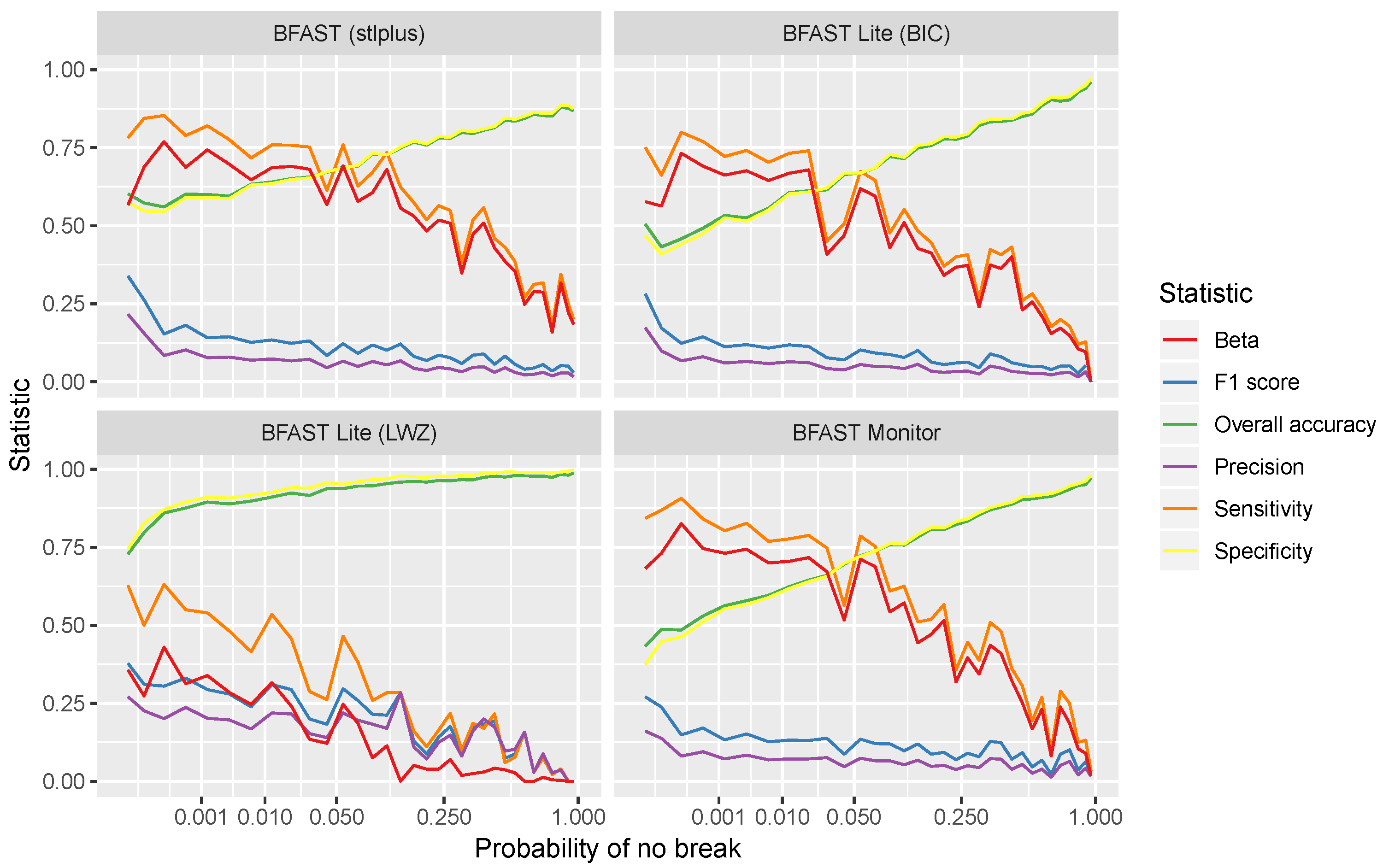
When looking further into the accuracy statistics and their change across the whole spectrum from high confidence of break in the time series to high confidence of no break in the time series, the results are given in Figure 3 for all of the reference data and in Figure 4 for reference points marked as a land cover change.
The results show that the statistics of all of the algorithms are close to one another and change consistently across the break confidence range. BFAST Lite with breakpoint number selection by LWZ is the only algorithm that stands out as different from the others. This shows that there is little difference between the algorithm results when comparable parameters (i.e., breakpoint selection by BIC) are used. However, the flexibility of BFAST Lite allows significant customisation of the algorithm when desired. When LWZ was used for selecting the number of breakpoints, it resulted in significantly better results: higher overall accuracy, F1 score, precision and specificity, as well as lower beta, throughout most of the range. However, it also had a lower sensitivity compared with other algorithms. This shows that break selection by LWZ makes the algorithm considerably more conservative, which means it does not overestimate the number of changes as often, albeit at the cost of some additional omission error.
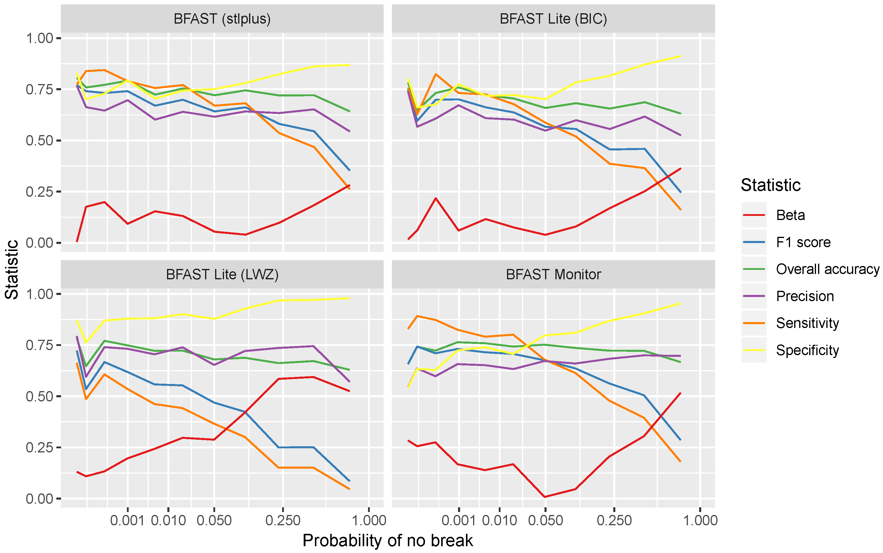
If we only consider locations marked as having a land cover change in any of the years in the reference data, we see the same pattern: all of the algorithms perform similarly except for BFAST Lite with LZW. However, in this case, BFAST Lite with break number selection by LWZ performed worse than with BIC. Since this dataset has a lot higher incidence of change, the conservative nature of the LWZ criterion results in a decrease in sensitivity that is not adequately compensated by the increase in precision. Since sensitivity is the limiting factor in this case, the use of LWZ also results in higher bias and a lower F1 score. In this case, all other algorithms had a higher F1 score and a lower beta statistic. BFAST achieved the highest F1 score and lowest beta throughout the range, but BFAST Lite with BIC had similar results as well.
3.2. Run Time Benchmark
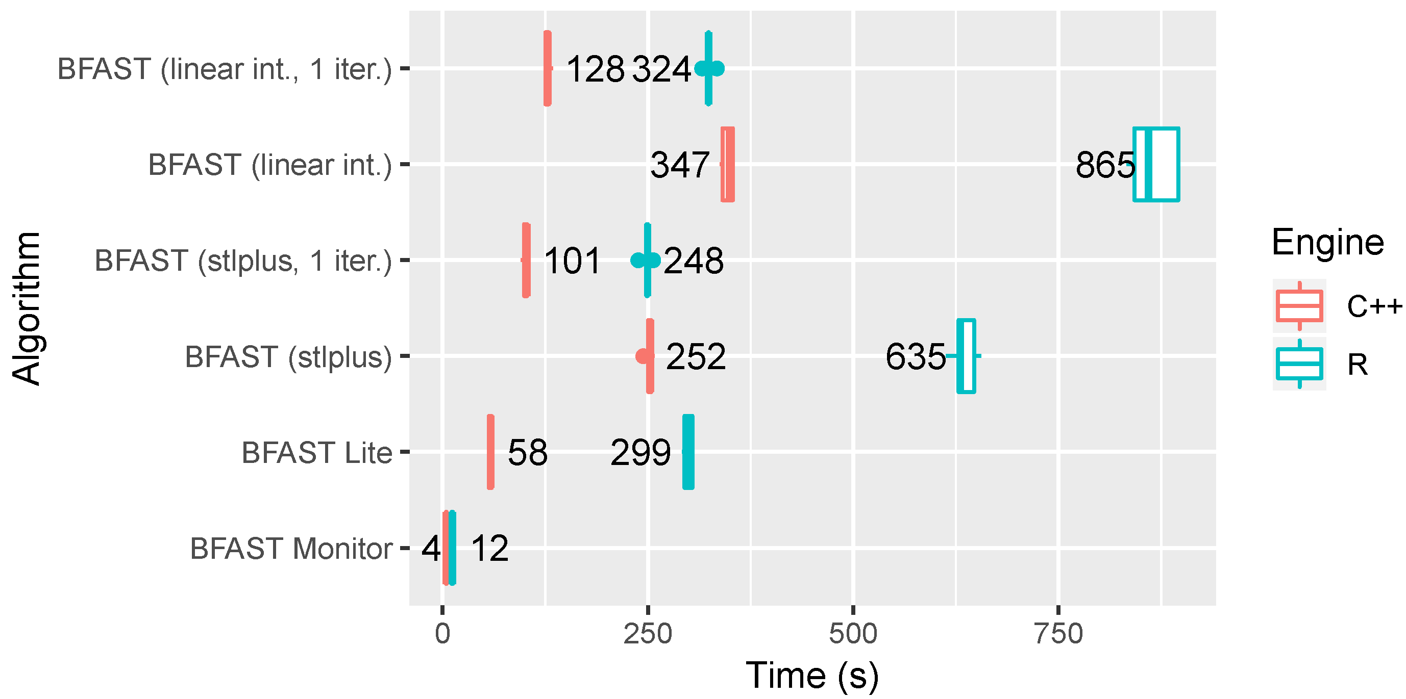
A summary of the run time benchmark results is shown in Figure 5. The results show that BFAST Lite run time when using the original R engine is comparable to BFAST when using a single iteration, but it is up to 2.9 times faster than BFAST using the original iterative approach. However, when using the optimised C++ engine, BFAST Lite is significantly faster than BFAST, regardless of the number of iterations. It was 1.7–2.2 times faster than BFAST using a single iteration and even 4.3–6.0 times faster than BFAST using the original iterative approach.
The C++ engine introduced in the new bfast release was faster than the R engine in all cases, with the gains consistently ranging between 2.5 and 3 times the speed of the R implementation.
Comparing the algorithms, BFAST was the slowest, and BFAST Monitor was the fastest. BFAST Monitor was 14.5 times faster than BFAST Lite and even 86.8 times faster than the original BFAST implementation when using the C++ engine. Comparing the two interpolation methods for BFAST, processing time series with stlplus interpolation was consistently faster by 1.3–1.4 times than using linear interpolation. This is because linear interpolation increases the number of observations that need to be processed by STL. Using a single iteration rather than an iterative approach in BFAST was 2.5–2.7 times faster consistently.
4. Discussion and Outlook
Our newly proposed algorithm, BFAST Lite, proved to be a useful addition to the existing family of BFAST algorithms. The results showed comparable accuracy with other BFAST algorithms and, in some cases, better than the original BFAST when comparable parameter settings were used. In addition, BFAST Lite was faster and more flexible than BFAST in terms of parameters. The additional parameters introduced in BFAST Lite proved to have a strong effect on the predicted time series breaks, which empowers users to customise the algorithm to fit their study area and use case. To avoid overloading users with too many adjustable parameters, all of the parameters were set as default to reasonable starting values for common tasks, such as forest disturbance detection. See Table A1 for a list of parameters and their default values. As a future research direction, it is planned to develop a supervised method for optimising parameters and the choice of the input vegetation index based on machine learning. Such a method would build upon the added parametrisation in BFAST Lite and could help users to automate its use for a wide variety of applications and locations.
The newly introduced LWZ criterion of BFAST Lite helps to reduce commission errors when the number of samples with no changes exceed the samples with land cover changes, which is usually the case due to the relative rarity of changes in land cover. The choice of the information criterion can shift the balance between commission and omission error drastically; therefore, selecting a criterion appropriate for a given task is important. We introduced the LWZ criterion due to its theoretical properties, as described in Liu et al. [23]. However, it is not necessarily optimal; information criteria other than AIC, BIC and LWZ may be better suited for specific tasks and result in a better balance between commission and omission error. Therefore, it is planned in upcoming releases of the package to allow users to pass a custom function to act as an information criterion, increasing the flexibility of the BFAST Lite algorithm further.
In addition to the aforementioned benefits, BFAST Lite also brings several more advantages over BFAST. First, it handles time series with missing values without the need for interpolation, unlike BFAST. Second, it provides additional metrics that can be used to further narrow down the detected changes: goodness-of-fit metrics, such as , RSS, BIC and LWZ, as well as several indicators for estimating the breakpoint magnitude. All of these features are practical benefits that ease the use of the algorithm and the interpretation of its output.
The faster speed of BFAST Lite means that it is now feasible to detect all breaks in time series over large areas, including running the algorithm globally. This was demonstrated in the production of the CGLS-LC100 maps [31], where BFAST Lite was used for reducing the number of changes between the yearly maps. BFAST Lite was run on the same set of MODIS imagery as presented in this study but globally and wall-to-wall. It was feasible to process the global time series data and produce a map of detected changes in approximately a week, running the algorithm on the Terrascope cluster, which provides approximately 1000 processor cores and 1.5 terrabytes of memory. To build upon these large-scale processing capabilities, BFAST Lite can further be ported to Google Earth Engine, similarly to BFAST Monitor [9]. This would allow running the algorithm over higher spatial resolution time series, such as Landsat, and would further ease the algorithm accessibility for a wider user audience.
Our study also showed good performance of BFAST Monitor compared to BFAST, even though BFAST Monitor was not designed for detecting multiple breaks. It is faster than BFAST Lite, and the accuracy is also comparable with BFAST. However, the limitation of BFAST Monitor is a high commission error. It is less suitable for dealing with data with relatively little change, as is the case at the global scale. See Table 2 for a summary comparison of the advantages and drawbacks of the three algorithms that we compared in this study.
Despite the recent advances in time series break detection, there is still a research gap remaining between the concepts of unsupervised break detection and land cover change detection. Since these concepts are not interchangeable, break detection algorithms alone are not enough to identify all types of land cover change. Therefore, more research is needed for improving land cover change detection. One approach is to use supervised algorithms. Such algorithms can make use of the output from unsupervised break detection algorithms, such as the BFAST family, as one of the inputs to help determine whether a land cover change has occurred. This approach was implemented by Xu et al. [34], who found that combining the output of two BFAST Lite models and one BFAST model in a Random Forest model increased the F1 score compared to BFAST Lite alone. This shows that BFAST Lite, due to increased flexibility and additional statistics on model fit and breakpoint magnitude, can help to further narrow down the detected breaks to those that actually correspond to land cover change.
5. Conclusions
We have introduced a new time series break detection algorithm, BFAST Lite, which is a faster and more flexible variant of the BFAST algorithm. The algorithm implementation in R is openly available in the bfast package version 1.6 on CRAN. BFAST Lite can handle missing data (irregular time series) and has a variety of user-customisable parameters, including the newly introduced LWZ information criterion for automatic determination of the number and timing of breakpoints. Our results showed that BFAST Lite performs similar to BFAST when using comparable parameters, with a higher user’s accuracy but a lower producer’s accuracy of change, and with a better balance between the two statistics. The choice of parameters has a big influence on the results, which allows tuning the model, e.g., decreasing commission errors when there is a lower incidence of change. In addition, BFAST Lite provides more statistics about the breakpoints and goodness-of-fit compared to other BFAST methods, which allows postprocessing of the results.
These outcomes, including the increased processing speed, show that BFAST Lite is a good candidate for upscaling break detection to larger areas. It has already been adopted in the production of the CGLS-LC100 product for annual land cover map updating at a global scale. BFAST Lite can help to detect disturbances on the ground and estimate their magnitude, as well as to determine long-term change trends, over larger areas than could previously be achieved with the original BFAST algorithm.
Author Contributions
Conceptualization, D.M., M.H., N.-E.T. and J.V.; methodology, J.V. and D.M.; software, D.M. and J.V.; validation, D.M.; formal analysis, D.M.; investigation, D.M. and N.-E.T.; data curation, D.M. and J.V.; writing—original draft preparation, D.M.; writing—review and editing, N.-E.T. and J.V.; visualization, D.M.; supervision, M.H., N.-E.T. and J.V.; project administration, M.H. All authors have read and agreed to the published version of the manuscript.
Funding
This research received no external funding.
Institutional Review Board Statement
Not applicable.
Informed Consent Statement
Not applicable.
Data Availability Statement
The software presented in this study is openly available under the GNU General Public License version 2 or later on GitHub at https://github.com/bfast2/bfast, accessed on 20 August 2021, as well as on Zenodo at https://0-doi-org.brum.beds.ac.uk/10.5281/zenodo.5018513, accessed on 20 August 2021. Restrictions apply to the availability of the land cover change reference data. Data were obtained from IIASA and are available from the authors with the permission of IIASA.
Acknowledgments
We thank Achim Zeileis for the initial ideas on the implementation of BFAST Lite and its break magnitude and for suggesting the LWZ criterion. We thank Marius Appel for the the C++ engine to speed up the functions in the bfast and strucchangeRcpp packages. We thank the CGLS-LC100 project (Bruno Smets, Marcel Buchhorn, Linlin Li, Agnieszka Tarko) for ideas and support. We thank IIASA (Myroslava Lesiv, Steffen Fritz) for providing us with land cover change reference data. We thank VITO and the Terrascope platform for MODIS data and computational facilities.
Conflicts of Interest
The authors declare no conflict of interest.
Abbreviations
The following abbreviations are used in this manuscript:
| AIC | Akaike’s Information Criterion. 3, 11 |
| BFAST | Breaks For Additive Season and Trend. 1, 2, 3, 4, 5, 6, 8, 9, 10, 11, 12, 14 |
| BIC | Bayesian Information Criterion. 3, 5, 9, 11 |
| CCDC | Continuous Change Detection and Classification. 1, 2 |
| CGLS-LC100 | Copernicus Global Land Services Land Cover 100 m. 3, 6, 13 |
| EWMACD | Exponentially Weighted Moving Average Change Detection. 1 |
| IIASA | International Institute for Applied Systems Analysis. 6, 13 |
| JUST | Jumps Upon Spectrum and Trend. 1 |
| LWZ | information criterion of Liu,Wu and Zidek. 3, 5, 8, 9, 11, 12, 13 |
| OLS-MOSUM | ordinary least squares residual moving sum. 3, 4, 6, 8, 10 |
| RSS | residual sum of squares. 3, 11 |
| STL | Seasonal decomposition of Time series by Loess. 3, 11 |
| TSCCD | Time-Series Classification approach based on Change Detection. 1 |
Appendix A

Table A1.
Comparison of parameters between BFAST and BFAST Lite.
| Parameter | BFAST | BFAST Lite |
|---|---|---|
| Minimum segment size h | 15% by default | 15% by default |
| Trend component | Always included | Included by default, can be disabled |
| Seasonality component | Either harmonics or seasonal dummies | Harmonics, seasonal dummies, both or external regressor |
| Maximum harmonic order | Preset to 3 | Customisable, defaults to 3 |
| Number of seasonal dummies | Preset to equal to observations per year | Customisable, defaults to the number of observations per year but can be fewer |
| Maximum number of iterations | 10 by default | 1 |
| Structural change test type | OLS-MOSUM by default | None, from version 1.7: optional with none by default |
| Structural change test significance threshold | 0.05 by default | None, from version 1.7: optional with 0.05 by default |
| Decomposition algorithm | STL by default or stlplus | None by default, STL or stlplus on any of the components |
| Break number selection criterion | Preset to BIC | LWZ by default, BIC, RSS |
| Autoregressive components | None (not supported) | None by default, seasonal lag, trend lag, or both |
References
- Kennedy, R.E.; Yang, Z.; Cohen, W.B. Detecting trends in forest disturbance and recovery using yearly Landsat time series: 1. LandTrendr—Temporal segmentation algorithms. Remote Sens. Environ. 2010, 114, 2897–2910. [Google Scholar] [CrossRef]
- Verbesselt, J.; Hyndman, R.; Newnham, G.; Culvenor, D. Detecting trend and seasonal changes in satellite image time series. Remote Sens. Environ. 2010, 114, 106–115. [Google Scholar] [CrossRef]
- Verbesselt, J.; Zeileis, A.; Herold, M. Near real-time disturbance detection using satellite image time series. Remote Sens. Environ. 2012, 123, 98–108. [Google Scholar] [CrossRef]
- Zhu, Z.; Woodcock, C.E. Continuous change detection and classification of land cover using all available Landsat data. Remote Sens. Environ. 2014, 144, 152–171. [Google Scholar] [CrossRef] [Green Version]
- Brooks, E.B.; Wynne, R.H.; Thomas, V.A.; Blinn, C.E.; Coulston, J.W. On-the-Fly Massively Multitemporal Change Detection Using Statistical Quality Control Charts and Landsat Data. IEEE Trans. Geosci. Remote Sens. 2014, 52. [Google Scholar] [CrossRef]
- Yan, J.; Wang, L.; Song, W.; Chen, Y.; Chen, X.; Deng, Z. A time-series classification approach based on change detection for rapid land cover mapping. ISPRS J. Photogramm. Remote Sens. 2019, 158, 249–262. [Google Scholar] [CrossRef]
- Ghaderpour, E.; Vujadinovic, T. Change Detection within Remotely Sensed Satellite Image Time Series via Spectral Analysis. Remote Sens. 2020, 12, 4001. [Google Scholar] [CrossRef]
- Kennedy, R.E.; Yang, Z.; Gorelick, N.; Braaten, J.; Cavalcante, L.; Cohen, W.B.; Healey, S. Implementation of the LandTrendr Algorithm on Google Earth Engine. Remote Sens. 2018, 10, 691. [Google Scholar] [CrossRef] [Green Version]
- Hamunyela, E.; Rosca, S.; Mirt, A.; Engle, E.; Herold, M.; Gieseke, F.; Verbesselt, J. Implementation of BFASTmonitor Algorithm on Google Earth Engine to Support Large-Area and Sub-Annual Change Monitoring Using Earth Observation Data. Remote Sens. 2020, 12, 2953. [Google Scholar] [CrossRef]
- De Jong, R.; Verbesselt, J.; Zeileis, A.; Schaepman, M.E. Shifts in Global Vegetation Activity Trends. Remote Sens. 2013, 5, 1117–1133. [Google Scholar] [CrossRef] [Green Version]
- Watts, L.M.; Laffan, S.W. Effectiveness of the BFAST algorithm for detecting vegetation response patterns in a semi-arid region. Remote Sens. Environ. 2014, 154, 234–245. [Google Scholar] [CrossRef]
- Fang, X.; Zhu, Q.; Ren, L.; Chen, H.; Wang, K.; Peng, C. Large-scale detection of vegetation dynamics and their potential drivers using MODIS images and BFAST: A case study in Quebec, Canada. Remote Sens. Environ. 2018, 206, 391–402. [Google Scholar] [CrossRef]
- Murillo-Sandoval, P.J.; Hilker, T.; Krawchuk, M.A.; Van Den Hoek, J. Detecting and Attributing Drivers of Forest Disturbance in the Colombian Andes Using Landsat Time-Series. Forests 2018, 9, 269. [Google Scholar] [CrossRef] [Green Version]
- Bernardino, P.N.; Keersmaecker, W.D.; Fensholt, R.; Verbesselt, J.; Somers, B.; Horion, S. Global-scale characterization of turning points in arid and semi-arid ecosystem functioning. Glob. Ecol. Biogeogr. 2020, 29, 1230–1245. [Google Scholar] [CrossRef] [Green Version]
- Burrell, A.L.; Evans, J.P.; Liu, Y. Detecting dryland degradation using Time Series Segmentation and Residual Trend analysis (TSS-RESTREND). Remote Sens. Environ. 2017, 197, 43–57. [Google Scholar] [CrossRef]
- Hamunyela, E.; Verbesselt, J.; Herold, M. Using spatial context to improve early detection of deforestation from Landsat time series. Remote Sens. Environ. 2016, 172, 126–138. [Google Scholar] [CrossRef]
- Cleveland, R.; Cleveland, W.; McRae, J.E.; Terpenning, I.J. STL: A seasonal-trend decomposition procedure based on LOESS (with discussion). J. Off. Stat. 1990, 6, 3–73. [Google Scholar]
- Bai, J.; Perron, P. Computation and analysis of multiple structural change models. J. Appl. Econom. 2003, 18, 1–22. [Google Scholar] [CrossRef] [Green Version]
- Jakubauskas, M.E.; Legates, D.R.; Kastens, J.H. Harmonic analysis of time-series AVHRR NDVI data. Photogramm. Eng. Remote Sens. 2001, 67, 461–470. [Google Scholar]
- Makridakis, S.G.; Wheelwright, S.C.; Hyndman, R.J. Forecasting: Methods and Applications, 3 ed.; Wiley: New York, NY, USA, 1997. [Google Scholar]
- Dutrieux, L.P.; Verbesselt, J.; Kooistra, L.; Herold, M. Monitoring forest cover loss using multiple data streams, a case study of a tropical dry forest in Bolivia. ISPRS J. Photogramm. Remote Sens. 2015, 107, 112–125. [Google Scholar] [CrossRef]
- Zeileis, A.; Kleiber, C.; Krämer, W.; Hornik, K. Testing and dating of structural changes in practice. Comput. Stat. Data Anal. 2003, 44, 109–123. [Google Scholar] [CrossRef] [Green Version]
- Liu, J.; Wu, S.; Zidek, J.V. On segmented multivariate regression. Stat. Sin. 1997, 7, 497–525. [Google Scholar]
- Shao, Q.; Campbell, N.A. Applications: Modelling trends in groundwater levels by segmented regression with constraints. Aust. N. Z. J. Stat. 2002, 44, 129–141. [Google Scholar] [CrossRef]
- Masiliūnas, D.; Verbesselt, J.; Zeileis, A.; Appel, M. bfast. Version 1.6.1; Zenodo: Genève, Switzerland, 2021. [Google Scholar] [CrossRef]
- Awty-Carroll, K.; Bunting, P.; Hardy, A.; Bell, G. An Evaluation and Comparison of Four Dense Time Series Change Detection Methods Using Simulated Data. Remote Sens. 2019, 11, 2779. [Google Scholar] [CrossRef] [Green Version]
- Hafen, R. Stlplus: Enhanced Seasonal Decomposition of Time Series by Loess; R Package Version 0.5.1. 2016. Available online: https://cran.r-project.org/web/packages/stlplus/stlplus.pdf (accessed on 20 August 2021).
- Dutrieux, L.P.; Jakovac, C.C.; Latifah, S.H.; Kooistra, L. Reconstructing land use history from Landsat time-series: Case study of a swidden agriculture system in Brazil. Int. J. Appl. Earth Obs. Geoinf. 2016, 47, 112–124. [Google Scholar] [CrossRef]
- Mersmann, O. Microbenchmark: Accurate Timing Functions; R Package Version 1.4-7. 2019. Available online: https://cran.r-project.org/web/packages/microbenchmark/microbenchmark.pdf (accessed on 20 August 2021).
- Badgley, G.; Field, C.B.; Berry, J.A. Canopy near-infrared reflectance and terrestrial photosynthesis. Sci. Adv. 2017, 3. [Google Scholar] [CrossRef] [Green Version]
- Buchhorn, M.; Bertels, L.; Smets, B.; Roo, B.D.; Lesiv, M.; Tsendbazar, N.E.; Masiliūnas, D.; Li, L. Copernicus Global Land Service: Land Cover 100 m: Version 3 Globe 2015–2019: Algorithm Theoretical Basis Document; Zenodo: Genève, Switzerland, 2021. [Google Scholar] [CrossRef]
- Zhou, X.; Del Valle, A. Range Based Confusion Matrix for Imbalanced Time Series Classification. In Proceedings of the 2020 6th Conference on Data Science and Machine Learning Applications (CDMA), Riyadh, Saudi Arabia, 4–5 March 2020; pp. 1–6. [Google Scholar] [CrossRef]
- Cohen, W.B.; Healey, S.P.; Yang, Z.; Stehman, S.V.; Brewer, C.K.; Brooks, E.B.; Gorelick, N.; Huang, C.; Hughes, M.J.; Kennedy, R.E.; et al. How similar are forest disturbance maps derived from different Landsat time series algorithms? Forests 2017, 8, 98. [Google Scholar] [CrossRef]
- Xu, L.; Herold, M.; Tsendbazar, N.E.; Masiliūnas, D.; Li, L.; Lesiv, M.; Fritz, S.; Verbesselt, J. Time series analysis for global land cover change monitoring: A comparison across sensors. in review.
Figure 1.
A schematic overview of the algorithms: (a) BFAST, (b) BFAST Lite. Dashed line indicates an optional step that is disabled by default. The breakpoint detection step [18] involves the following substeps: the generation of components for model fitting, fitting the model itself, determining all possible breakpoints and selecting an optimal number of breakpoints.

Figure 2.
Locations of all land cover change reference sites. Each site covers a 300 by 300 m area, aligned with the PROBA-V 300 m UTM grid, and indicates whether more than 50% of this area underwent a land cover change between each pair of years between 2015 and 2018. Sites with at least one year of land cover change are marked in red, others in green. Background: World Bank Official Boundaries.

Figure 3.
Algorithm accuracy comparison across the range of confidence in the time series having at least one break (i.e., ordinary least squares residual moving sum (OLS-MOSUM) test p-value) among the entire reference data set. Towards the left on the x axis are time series with high confidence of a break and towards the right with a high confidence of no break. The data are binned to ∼1000 locations per bin.

Figure 4.
Algorithm accuracy comparison across the range of confidence in the time series having at least one break (i.e., OLS-MOSUM test p-value) among time series that have at least one land cover change event. Towards the left on the x axis are time series with high confidence of a break and towards the right with a high confidence of no break. The data are binned to ∼300 locations per bin.

Figure 5.
The run time benchmark between the tested algorithms. Each algorithm has been run 5 times on a dataset of 288 time series. The time axis represents the total time needed to process this dataset. “1 iter.” indicates that the algorithm was run for a single iteration rather than iteratively, and “linear int.” indicates filling in missing data using linear interpolation.

Table 1.
Accuracy statistics of the tested algorithms. “OA” stands for overall accuracy.
| Algorithm | Sensitivity | Specificity | Precision | F1 score | OA | Beta |
|---|---|---|---|---|---|---|
| BFAST Lite (BIC) | 0.737 | 0.881 | 0.607 | 0.666 | 0.852 | 0.130 |
| BFAST Lite (LWZ) | 0.569 | 0.943 | 0.715 | 0.633 | 0.868 | 0.146 |
| BFAST (linear int.) | 0.880 | 0.807 | 0.518 | 0.653 | 0.821 | 0.362 |
| BFAST (stlplus) | 0.811 | 0.832 | 0.540 | 0.648 | 0.827 | 0.271 |
| BFAST Monitor | 0.852 | 0.851 | 0.587 | 0.695 | 0.851 | 0.265 |
Table 2.
Feature comparison between the three BFAST family algorithms. See Table A1 for a detailed comparison of parameters between BFAST and BFAST Lite.
Table 2.
Feature comparison between the three BFAST family algorithms. See Table A1 for a detailed comparison of parameters between BFAST and BFAST Lite.
| Algorithm | Advantages | Disadvantages |
|---|---|---|
| BFAST [2] | Detects breaks in trends and seasonality separately | Slow, limited number of parameters, overestimates change |
| BFAST Monitor [3] | Designed to detect breaks at the end of time series (near real-time), fastest, many tunable parameters | By default not designed for multiple breakpoints, overestimates change |
| BFAST Lite (this study) | Faster than BFAST, designed for multiple breakpoints, many tunable parameters, lowest bias between sensitivity and precision, highest OA | Needs parameter tuning to optimise performance, does not differentiate between breaks in seasonality and trend |
Publisher’s Note: MDPI stays neutral with regard to jurisdictional claims in published maps and institutional affiliations. |
© 2021 by the authors. Licensee MDPI, Basel, Switzerland. This article is an open access article distributed under the terms and conditions of the Creative Commons Attribution (CC BY) license (https://creativecommons.org/licenses/by/4.0/).
Share and Cite
MDPI and ACS Style
Masiliūnas, D.; Tsendbazar, N.-E.; Herold, M.; Verbesselt, J. BFAST Lite: A Lightweight Break Detection Method for Time Series Analysis. Remote Sens. 2021, 13, 3308. https://0-doi-org.brum.beds.ac.uk/10.3390/rs13163308
AMA Style
Masiliūnas D, Tsendbazar N-E, Herold M, Verbesselt J. BFAST Lite: A Lightweight Break Detection Method for Time Series Analysis. Remote Sensing. 2021; 13(16):3308. https://0-doi-org.brum.beds.ac.uk/10.3390/rs13163308
Chicago/Turabian StyleMasiliūnas, Dainius, Nandin-Erdene Tsendbazar, Martin Herold, and Jan Verbesselt. 2021. "BFAST Lite: A Lightweight Break Detection Method for Time Series Analysis" Remote Sensing 13, no. 16: 3308. https://0-doi-org.brum.beds.ac.uk/10.3390/rs13163308
Note that from the first issue of 2016, this journal uses article numbers instead of page numbers. See further details here.