
LSTM-Based Remote Sensing Inversion of Largescale Sand Wave Topography of the Taiwan Banks


1
School of Computer Science and Technology, Hangzhou Dianzi University, Hangzhou 310018, China
2
State Key Laboratory of Satellite Ocean Environment Dynamics, Second Institute of Oceanography, Ministry of Natural Resources, Hangzhou 310012, China
*
Author to whom correspondence should be addressed.
Remote Sens. 2021, 13(16), 3313; https://0-doi-org.brum.beds.ac.uk/10.3390/rs13163313
Submission received: 8 June 2021
/
Revised: 17 August 2021
/
Accepted: 18 August 2021
/
Published: 21 August 2021
(This article belongs to the Special Issue GIS and RS in Ocean, Island and Coastal Zone)
Abstract
:Shallow underwater topography has important practical applications in fisheries, navigation, and pipeline laying. Traditional multibeam bathymetry is limited by the high cost of largescale topographic surveys in large, shallow sand wave areas. Remote sensing inversion methods to detect shallow sand wave topography in Taiwan rely heavily on measured water depth data. To address these problems, this study proposes a largescale remote sensing inversion model of sand wave topography based on long short-term memory network machine learning. Using multi-angle sun glitter remote sensing to obtain sea surface roughness (SSR) information and by learning and training SSR and its corresponding water depth information, the sand wave topography of a largescale shallow sea sand wave region is extracted. The accuracy of the model is validated through its application to a 774 km2 area in the sand wave topography of the Taiwan Banks. The model obtains a root mean square error of 3.31–3.67 m, indicating that the method has good generalization capability and can achieve a largescale topographic understanding of shallow sand waves with some training on measured bathymetry data. Sand wave topography is widely present in tidal environments; our method has low requirements for ground data, with high application value.

1. Introduction
Extensive sand wave topography is distributed in tidal environments worldwide, such as the North Sea in Europe [1], the South Sea in Korea [2], San Francisco Bay in the Americas [3], and shallow shoals in Taiwan, China [4]. The study of sand wave shoal topography forms an important basis for coastal protection [5], navigation safety [6], submarine pipeline laying, and drilling platform construction [7]. The shallow sand wave topography of the Taiwan Banks, located offshore, is the largest sand wave shallow topography in the world [4]. The sand wave water depths are roughly distributed between 20 and 60 m [8], and water turbidity makes it difficult for sunlight to penetrate the seafloor, rendering seafloor reflectivity-based detection methods unsuitable [9]. Currently, there are three methods that can be used for sand wave shallow terrain detection: sonar multibeam bathymetry [10], synthetic aperture radar (SAR) detection, and sun glitter remote sensing. Among them, multibeam bathymetry uses vessels as the detection platform and has high efficiency, accuracy, and resolution in detecting trajectories. However, the scanning width is extremely limited, the coverage area is small, the measurement period is long, and the manpower and financial requirements are high [11].
Both SAR sounding and sun glitter remote sensing are ocean dynamics sounding techniques based on sea surface roughness (SSR) and are not constrained by seawater turbidity. They can be operated at large depths [12] and have a wide range of applications. A model for detecting shallow underwater topography (AH model) was developed using SAR sounding data [13]. A bathymetry assessment system (BAS) was built based on the AH model, and it achieved an inversion accuracy of 30 cm in the shallow sand wave region of the Dutch North Sea [14]. An SAR shallow sounding model based on the AH model achieved a 42 cm inversion accuracy [15]. SAR image simulation using the M4S software (a model for full two-dimensional simulation) achieved a 3.04 m accuracy for shallow sand waves in the Taiwan Banks [10]. The development of sun glitter remote sensing has lagged compared to SAR detection. Hennings et al. [16] found light and dark streak variations in underwater topography in the infrared band remote sensing images from Skylab, with the underlying cause possibly being the modulation of the image signal by underwater topography. The imaging theory for shallow sandy wave topography in sun glitter remote sensing was developed based on a synthesis of the AH model and the relationship between the tilted wave surface probability and sea surface wind field generalized by Cox et al. [17] and the CM model [18]. For example, Shao et al. [19] applied a pendulum equation fitting method to obtain a root mean square error of 4.2 m on typical sand wave sections and confirmed the existence of a one-to-one progressive modulation relationship between underwater topography, surface flow field, and SSR. On the other hand, He et al. [20] combined multibeam bathymetry data and sand ridge line information from sun glitter images to achieve an inversion accuracy of 1.37 m for a sand wave topography reconstruction experiment in a cell. However, their attempts focused on sand wave sections or small areas and relied heavily on measured data. It is difficult to apply these data at a large scale; thus, they are unfit for use in the sand wave distribution area of the Taiwan Banks, with a total area of 16,000 km2 [8].
The development of deep learning is transforming learning across all disciplines, and the application of neural networks allows us to obtain reliable inversion results, including in the field of bathymetry. For example, Liu et al. [21] used a local neural network algorithm to derive water depth data from optical images. Alevizos et al. [22] used hyperspectral imagery combined with machine learning for bathymetric sounding. Panagiotis et al. [23] performed bathymetric sounding based on accurate aerial photography and machine learning. These studies have yielded good results, but they focused on the shallow sea domain. A large number of studies have shown that, in sand wave topography, sun glitter SSR and water depth vary in the same cycle in the direction vertical to the sand ridge line [19,24], and that this relationship can be mapped to a temporal relationship. In other words, the field of bathymetry changes continuously and periodically, not only in relation to current features, but also with respect to previous bathymetric sequences. Long short-term memory (LSTM) networks are able to use long time-series information [25] to complete model construction, and this method is widely used in other fields with periodic time-series characteristics. For example, the long-term value of soil moisture active passive (SMAP) was estimated using LSTM networks [26]. Similarly, the sea temperature in Chinese offshore areas was predicted using RC-LSTM networks [27]. Wang et al. [28] developed a long- and short-term memory-based model to reconstruct water storage changes in the Tarim River basin. Zhang et al. [29] combined optical, thermal satellite, and environmental data to predict county-level maize yields in China using LSTM networks.
Previous methods for bathymetry detection are either difficult to transmit to the water bottom, such as inversion based on seafloor reflectivity, or economically unfeasible, such as sonar-based multibeam detection. SSR-based methods can be used for sand wave topography detection in Taiwan Banks, also heavily dependent on measured water depth. These measured data are only effective for calculating the inversion of areas near the measured water depths, and it is difficult to obtain terrain information for large areas of sand waves far from the measured line using them. Consequently, previous sun glitter studies have been unable to detect the large areas of sand wave topography over the entire Taiwan Banks area. In this study, we constructed a shallow beach sand wave inversion model based on LSTM networks using the characteristics of the sand wave topography, relying negligibly on actual measurement data. This enabled easy detection and allowed the model to be extended to a large scale. First, multi-angle sun glitter remote sensing images were used to obtain high-resolution SSR information. A region with available measured water depth was selected, and the surface roughness and measured water depth were input into the LSTM model for training. Afterward, the trained model was applied to other areas to obtain the bathymetry of the inversion area. Finally, the model was validated using navigational survey lines to observe the migration capability of the model. The accuracy of the model and the factors affecting the accuracy were analyzed. The remainder of this paper is organized as follows: Section 2 introduces the study area and data sources and analyzes the mapping of water depth and roughness to time-series features. Section 3 introduces the LSTM model, data processing methods, and the training and inversion of the LSTM model. Section 4 analyzes the results of the experiments and the results applied to other regions. Section 5 discusses the results of the inversion. Finally, Section 6 concludes the paper.
2. Study Area Profile and Dataset
2.1. Study Area
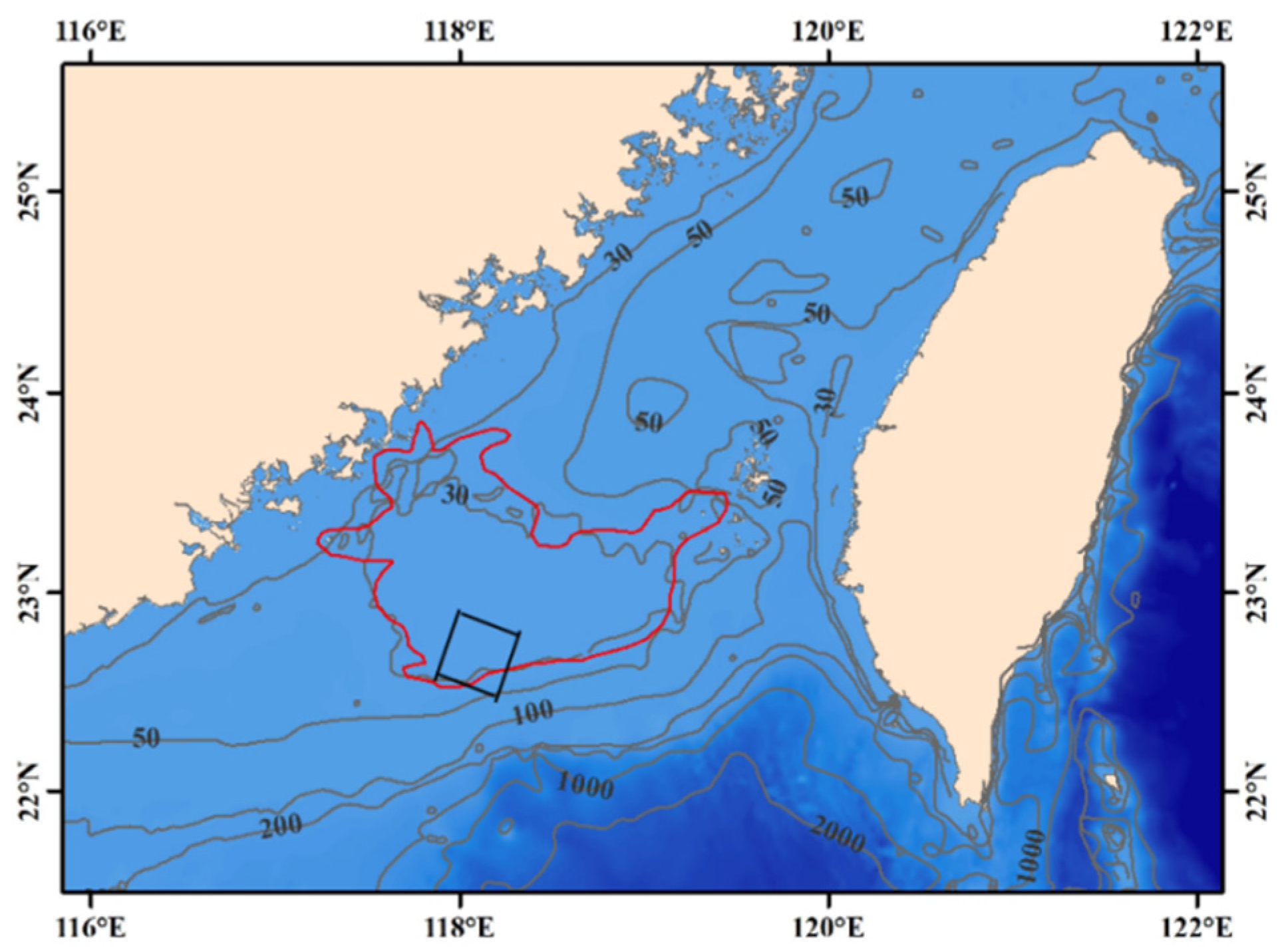
Marine areas with strong hydrodynamics and sufficient sand sources typically develop a rhythmic bottom bed morphology. The study area located in the southern Taiwan Strait is the world’s largest submerged sand wave system [4]. As shown in Figure 1,the Taiwan Shoal extends from 117°14 to 119°26E and from 22°32.5 to 23°49N, spanning 228 km from east to west and 145 km from north to south. A total of 16,400 km2 of the Taiwan Shoal, indicated by the red boundary in Figure 1, was observed using remote sensing imagery [8]. The sand wave directions (0° due north) are distributed between 132° and 264°, with a statistically normal trend. The probability of wave directions at 180° is the highest, and the sand ridge direction is primarily oriented east to west. The wavelengths of the sand waves in the Taiwan Banks range from 76 m to 2151 m, with a statistical mean wavelength of 721 m. Ridge lengths range from 254 to 19,992 m, while most are shorter than 3000 m, with a statistical mean ridge line length of 2453 m. The morphology of shallow sand waves is relatively diverse, with types including double-peaked sand waves, cosine sand waves [30], and pendulum sand waves [31]. The amplitude of sand waves in the Taiwan Banks is approximately 10 m, and the average water depth is approximately 20 m.
2.2. Dataset
In this study, the SSR inversion model based on multi-angle sun glitter, proposed by Zhang et al. [32], was used to invert the multi-angle sun glitter data obtained from the 3N and 3B channels of ASTER remote sensing, imaged on 16 July 2003. The inversion obtained the same SSR data with a resolution of 15 m as in [32]. ASTER is an advanced multispectral imager, and the ASTER visible NIR subsystem has three bands. The sky bottom telescope image (NVI) of channel 3N has the same bandwidth as the rear-view image (BVI) of channel 3B. The high spatial resolution (15 m), the tilt capability of the sensor, and the rear-view angle of channel 3B render the ASTER imager considerably advantageous for marine applications involving multiple angles. The location depicted in Figure 2 at the Taiwan Shoal is indicated by the black box in Figure 1.
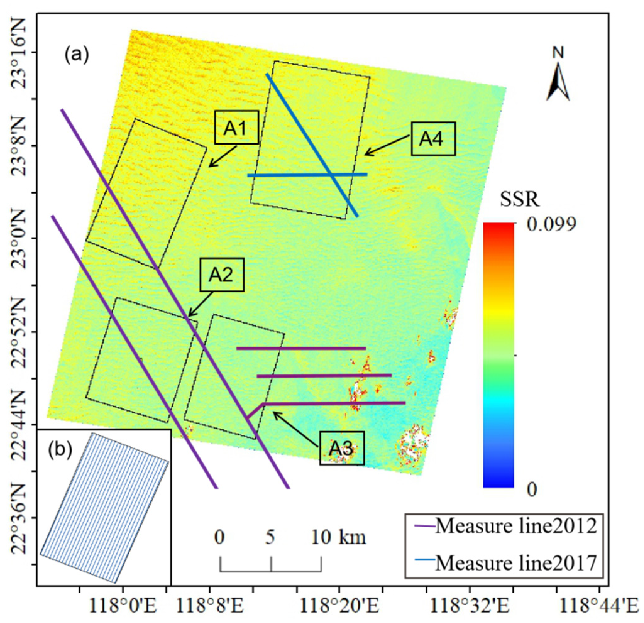
In addition, this study also employed measured bathymetry data obtained using multibeam bathymetry methods in August 2017 and May 2012, as indicated by the blue and purple line segments, respectively, in Figure 2. In the May 2012 survey, 25 measured bathymetric lines occur at 500 m intervals in area A1 in Figure 2b. The small interval between the measured lines was filled using the joint interpolation method in [20] as the whole training area. They were interpolated from a dense set of measured points and fed into the model as real terrain for training. Areas A2, A3, and A4 have measured lines crossing them, as shown in the figure. These multibeam bathymetry data were acquired using the R2 Sonic 2024 multibeam bathymetry system. The system is a fifth-generation physical multibeam system and can be used for the topographic mapping of the seabed at water depths of 1–500 m. The operating frequency was adjustable between 200 and 400 kHz, coverage width was 10° to 160°, and beam angle was 0.5° × 1°. In total, 256 effective detection beams could be formed, and the resolution was 1.25 cm. The measured bathymetry data with an average distance of 5 m were obtained after the sounding, and the measured bathymetry resolution was also reconstructed to 15 m according to the method of He in [20], which was kept uniform with the remote sensing data. According to Zhou et al. [4], in the Taiwan Banks, large sand waves do not migrate and sediments only move along the wave crests, and we affirm that the remote sensing data and measured bathymetry data correspond with this.
2.3. Sand Wave Terrain Feature Analysis
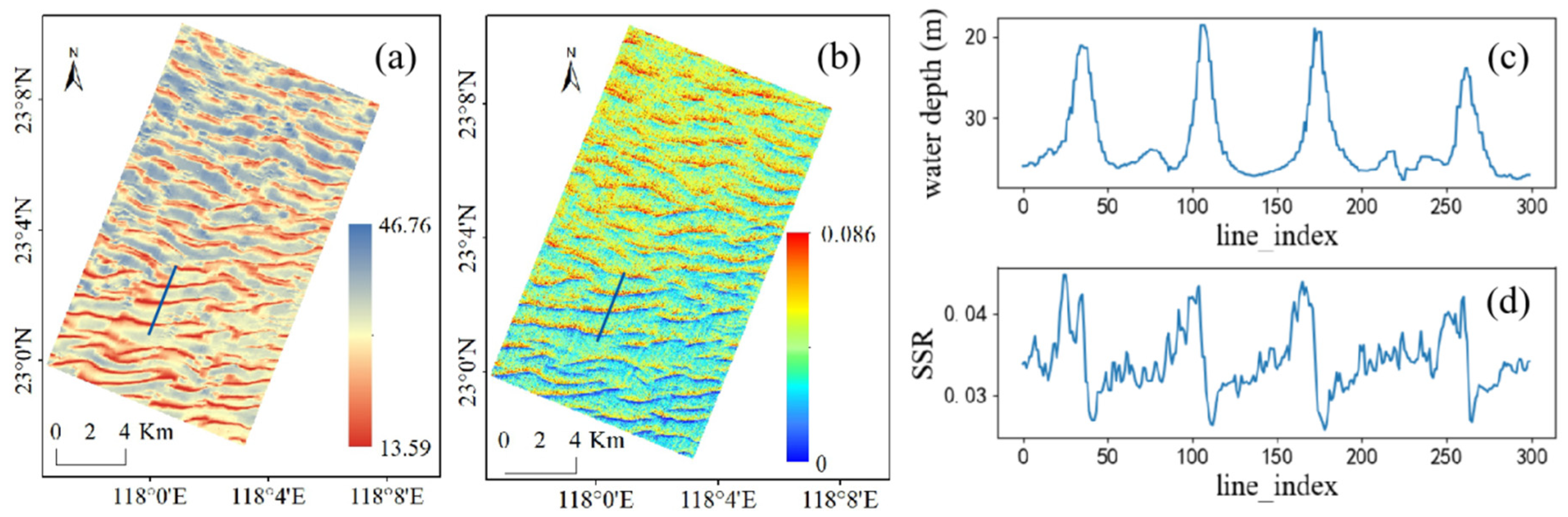
To explore both the general characteristics of the sand waves and roughness, we considered the profile line characteristics of the sand wave topography and SSR, respectively. The strongest signal variation was found perpendicularly to the sand ridge line. As shown in Figure 3a,b, a section of the profile lines was considered perpendicularly to the sand ridge line, and the variations in SSR and water depth were obtained as shown in Figure 3c.
Figure 3c shows that along the direction perpendicular to the sand ridge line, both SSR and bathymetry showed the same period of fluctuation; however, both showed different characteristics of variation. The peaks and troughs were interspersed, and the variations in bathymetry were always continuous, with the bathymetry at one point being closely related to that of the surrounding areas. The surface roughness modulated by the sand wave topography varied with the same periodicity as the topography; however, its lightness and darkness did not correspond with the bathymetry data, and a comparison of spatial locations revealed a sudden change in surface roughness at the crest of the sand wave.
The sequence characteristics displayed by the above-mentioned SSR and sand wave topography are similar to those of contextual sequences and periodic time sequences. Text sequences, for example, indicate contextual relevance [33]; weather conditions on consecutive days have some connection with those over past days [34]. The average wavelength of the sand waves in the Taiwan Banks is 721 m [8] and is characterized by long sequences. In this study, we introduce an LSTM neural network, a time-series model for long sequences, to find the continuous and periodic variation characteristics of SSR and sand wave topography in space, and to establish a prediction model to realize the remote sensing inversion of largescale sand wave topography.
3. Models and Methods
3.1. Methods Flow
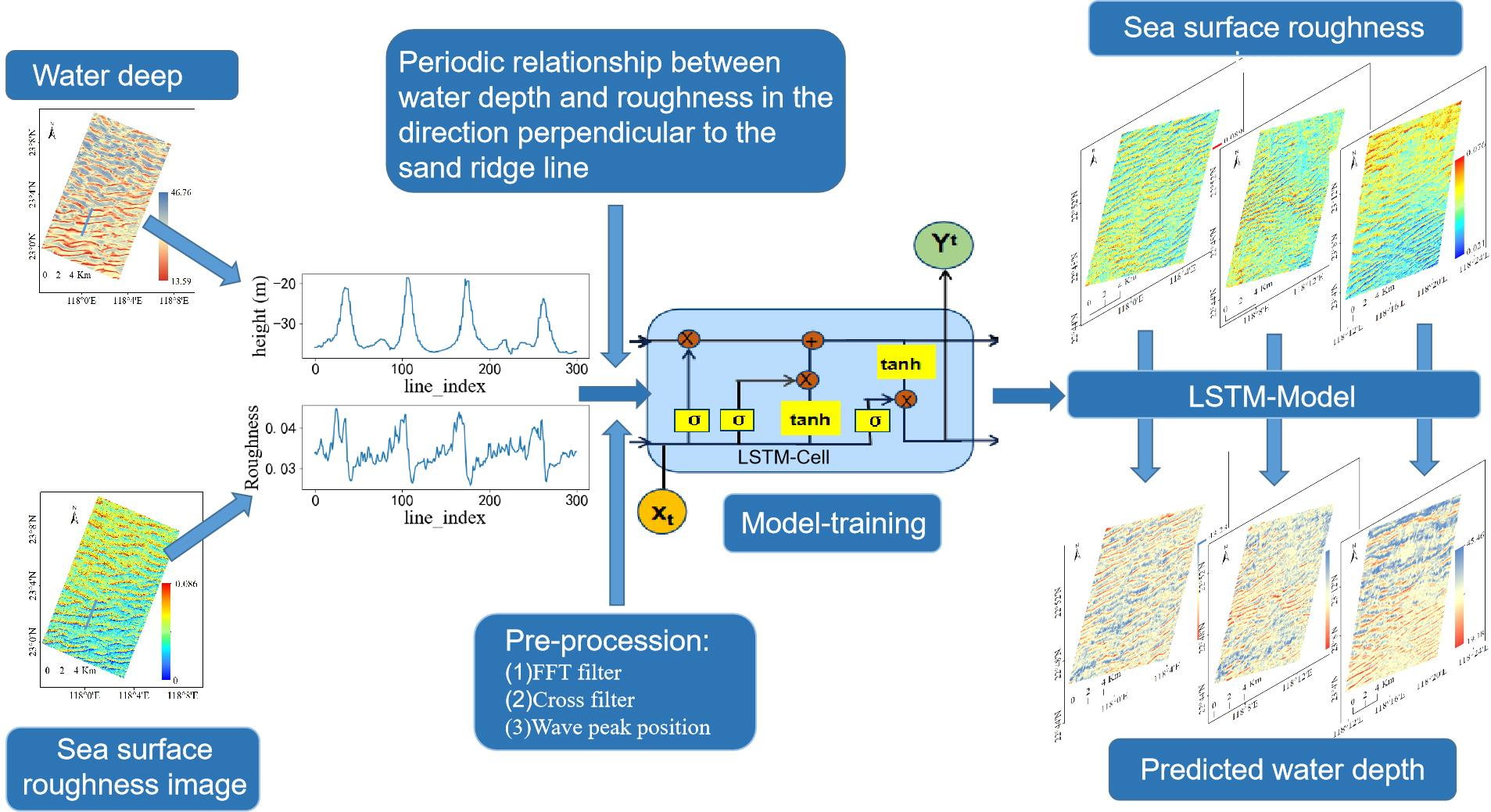
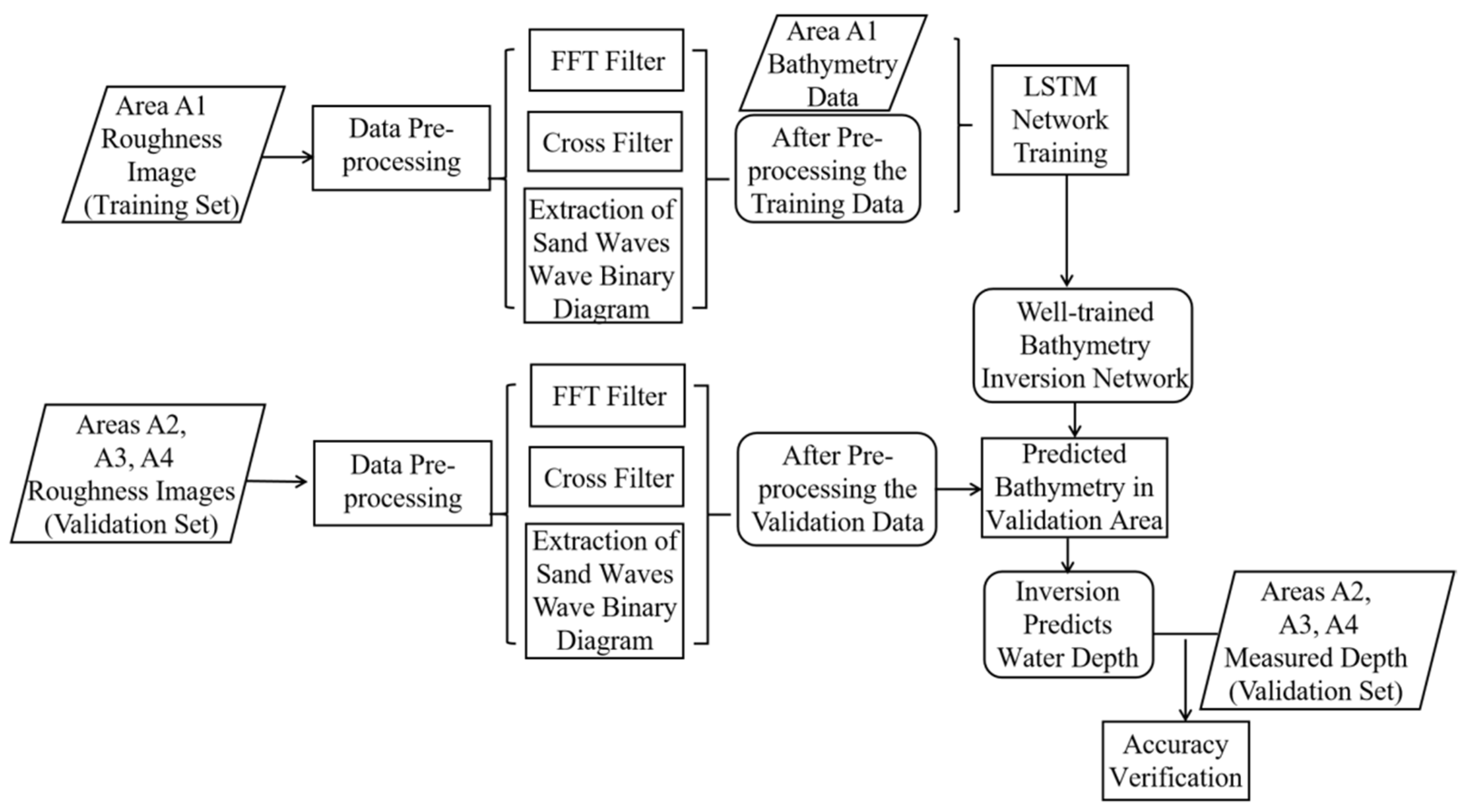
SSR is not only modulated by underwater topography, but also by the wind field at the sea surface [32]. We extracted the SSR sequence modulated by underwater topography as the input data corresponding to the respective bathymetric sequence. Next, we used a reasonable filter sequence to process the wind streaks and enhance data abundance. We subjected the original roughness image to fast Fourier transform (FFT) filtering and cross filtering, extracted the sand ridge line data to calibrate the location of the sand wave crest using the algorithm, and combined the three as input features to build a bathymetric inversion model through LSTM network training. In Figure 2, an iterative training model for A1 (255 km2) area for accuracy verification is presented. The trained inversion model was used to calculate the water depths in the A2 (224 km2), A3 (202 km2), and A4 (348 km2) areas, and the track survey line was used for verification. A flow chart detailing the entire experiment is shown in Figure 4.
3.2. Preprocessing of Data
3.2.1. Roughness Filtering
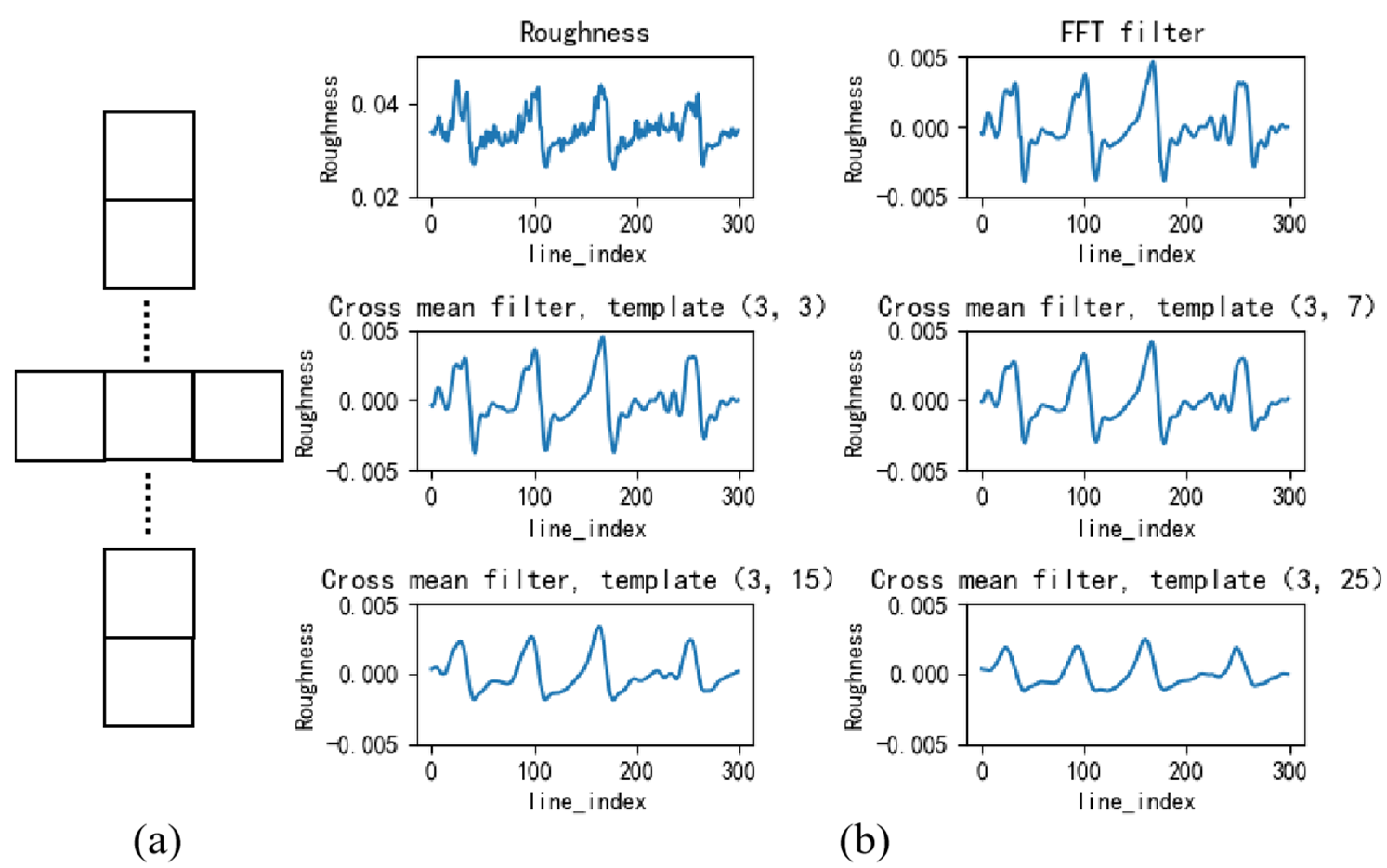
First, the effect of wind streaks on the accuracy of the terrain inversion by FFT filtering was excluded during preprocessing. Converting the roughness image from the spatial domain to the frequency domain revealed a significant difference in direction between the roughness modulated by the underwater terrain and that affected by the wind field. Data on the characteristic wavelengths and directions of the sand waves were selected in the frequency domain for FFT inversion transformation, and the results obtained are shown in the second image in Figure 5b. Thus, sand wave information was highlighted, and the effect of wind streaks was largely eliminated.
The second step of preprocessing involved mean filtering with a series of cross windows to determine the relationship between the variations in the two sequences of roughness and water depth at different scales, and the data were then fed into the LSTM model as supplementary data for training the model. The shape of the cross-filtered window is shown in Figure 5a, which beneficially retained similar water depth in the horizontal direction and reduced the streaking in the inversion results. After experimental validation, we identified four sets of cross-filter templates, namely (3,3), (3,7), (3,15), and (3,25). Figure 5b shows the results of the original roughness, FFT filtering, and four sets of cross-mean filtering assessments of the blue line profile in Figure 3a.
3.2.2. Sand Wave Crest Position Characteristics
The location of the sun glitter brightness and darkness reversal was the sand ridge line [19]. Precise extraction of sand ridges has been shown to facilitate the identification of wave crests. To retain sand wave crest information more precisely, we used the Canny operator [34] to extract the sand ridge line data. The results are presented as a binary map.
3.3. Construction of Inverse Models Based on LSTM Networks
3.3.1. LSTM Networks
LSTM neural networks are a good solution to the problem of gradient disappearance and gradient explosion that can occur in recurrent neural networks when learning over long sequences [24,35]. The basic unit of an LSTM network implicit layer is called a storage block, and its structure is shown in Figure 6.
The memory block contains the forget gate (f), input gate (i), output gate (o), and memory cell (C). All three gating structures are identical and are implemented by the sigmoid neural layer dot product operation, and the elements of the sigmoid layer output take values in the range [0, 1], indicating the weight required to let the corresponding message through. The symbol represents the dot product operation of two vectors; ⊕ represents the addition operation of two vectors; σ represents the sigmoid activation function; tanh is the hyperbolic tangent activation function; and x represents the input value. σ and tanh were calculated as follows.
The following characterized the flow of information in the LSTM storage block.
- Forget Gate:
- 2.
- Input Gate:
- 3.
- Output Gate:
- 4.
- Input Node:
- 5.
- Cell State:
- 6.
- Hidden Gate:
Wf, Wi, Wo, and Wc represent the weight vectors of the forget gates, input gates, output gates, and memory cells, respectively; bf, bi, bo, and bc represent the bias vectors of the forget gates, input gates, output gates, and memory cells, respectively; and Xt denotes the input to the t-node network.
The forget gate determined how historical information was retained; input gates determined how information from the input layer was passed to the memory unit; and output gates determined how information from the memory module was passed to the next moment of the storage block. Gate controllers described the proportion of messages that could pass through, and the σ function took values in the range [0, 1]. ft, it, and ot are the outputs of the t-node σ function; is the output of the tanh function at node t, taking values in the range [−1, 1]. After the input sequence had been gated as described above, the t-node long-term memory (Ct) and short-term memory (ht) were obtained and passed into the next memory block. In addition, ht was the output of node t (t = 1, 2, 3,…, n).
3.3.2. Training of LSTM Networks
The model was developed to minimize the distance between the predicted and actual water depths, and we used the root mean square error (RMSE), which is the distance between the two, as the indicator of the loss function. The updating of parameters, such as the weight vector (W) and the bias vector (b), during the training of the LSTM model depended not only on the current node but also on the previous node; this process is called back propagation in time (BPTT) [36]. In this process, the error derivatives are updated as time propagates, and matrices W and b are updated separately. In the experiment, the comparison of various gradient descent methods, such as Adam and SGD, revealed that the Adam algorithm had the highest accuracy. Thus, we used the Adam algorithm to update the parameters in our study.
The data obtained from preprocessing were used as input data and expressed as X = {Xt}.t = 1,2,3,..., n with Y = {Yt}.t = 1,2,3,..., n, where t denotes the input data at position t and contains one set of FFT-filtered data, four sets of cross-filtered data on roughness, and one set of binary map data. The predicted water depth data obtained from Xt are denoted as ht, and Yt denotes the actual water depth at position t. Given the window length L of the network, this parameter represents the prediction of the water depth at the end, based on an input sequence of length L. Xt,Xt+1……Xt+L−1 predicts the water depth at the end ht+L−1. The topology of the neural network determined from L is shown in Figure 7, where LSTMt denotes an LSTM storage block at position t.
Using this LSTM neural network structure, the input and output data were trained and predicted, respectively, using the following training process:
- (1).
- Two-dimensional images were transformed into one-dimensional images. To simulate continuously changing time streams, we connected the profile lines perpendicularly to the sand ridgeline according to the head and tail of the column. Correspondingly, we connected the topographic data head to tail along the profile lines. At this point, the two-dimensional image was converted into a one-dimensional continuous sequence of data.
- (2).
- Data normalization: The LSTM model learned the relative trends of two sequences, and, therefore, the Xt and yt data needed to be normalized. Their means were subtracted from both, and they were divided by the variance to obtain the final data set. The normalized depth value of the region was obtained by subtracting water depth data from the mean and dividing it by the variance.
- (3).
- Network initialization: The weights (W) and bias vector (b) were set to 0 at initialization. hidden_size was set to indicate the number of hidden layer storage block dimensions. The mid layer was set to indicate the number of hidden layers contained in the network. L indicated the input window length, and Lr indicated the step length of each random gradient descent.
- (4).
- Data partitioning: The dataset was divided into a training set Xtr = {X1,X2,… Xd} and a test set Xte′ = {Xd+1, Xd+2,…, Xn}. The training set was a subset organized according to the window length L. Each subset obtained was called a batch and was counted as {Xtr1,Xtr2,…,Xtrt,…,Xtrd-L+1}, where Xtrt = {Xt,Xt+1,…,Xt+L−1} is the primary input to the LSTM network, and its corresponding output is {ht,ht+1,…,ht+L−1}, which is counted as an epoch according to the number of rounds of the network iteration.
- (5).
- The key steps in training the LSTM model are presented in Algorithm 1.
| Algorithm 1: LSTM model iteration |
| Require: the initial value of W and b, number of hidden layers mid_layer, number of hidden layer storage block dimensions hidden_size, input window length L. for k = 1, 2,…Epoch do for t = 1,2,d + L − 1 do Calculate ft Get output ht end for Error calculation: E = (ht − yt)2 Calculate the Mean Square Error between the node output and the true value Node parameter update: Update W and b based on the error term E using the Adam gradient optimization algorithm. end for |
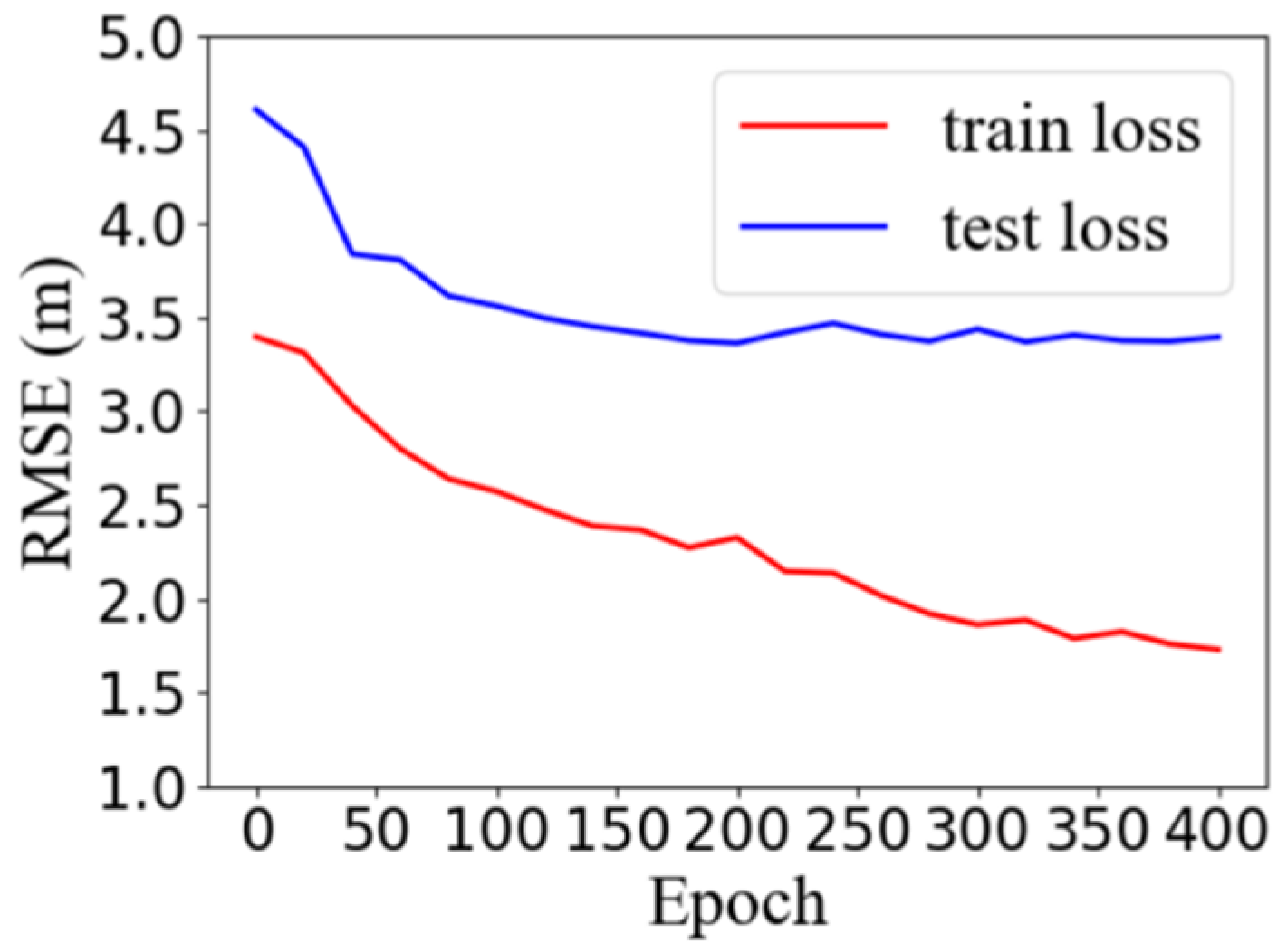
The optimal model was trained by adjusting the window length (L), the number of hidden layers (mid_layer), the number of nodes (hidden_size), the learning rate (Lr), and the number of epochs (epoch). Results were obtained when L was the column length of the training area, mid_layer was 4, hidden_size was 16, and Lr was 0.002. The accuracy of the model with iterations is shown in Figure 8. The horizontal coordinates indicate the number of iterations, and the vertical coordinates indicate the RMSE. The model remained largely stable.
3.4. Validation and Application
After the training had been completed, the trained network was used to iterate the predictions, using the following process:
The first dataset (Xte1) of the test set was taken and merged with the last L−1 values of Xtrd−L+1 to form a new subset {Xd−L+1, Xd−L+2, …, Xd, Xte1}. This subset was input into the network to obtain the first prediction of the validation set, hte1. The process was repeated to obtain the final prediction {hte1, hte2, …, hten}.
The data were normalized before being fed into the network by subtracting the value of the mean divided by the variance from both the input and output values. The image data were stitched into one dimension by column. After the normalized water depth data had been outputted from the network, the variance was multiplied by the mean to obtain the predicted water depth, and the predicted water depth was stitched into a topographic image by column.
The model was trained iteratively in the training area in region A1 shown in Figure 2, and accuracy validation was performed in the test area. The first 75% of the data were selected as the experimental set and the last 25% as the validation set, and good inversion results were obtained. The generalization ability of the model was tested by adjusting the training and test sets. Two parameters, the mean absolute value error (MAE) and the RMSE, were used to characterize the accuracy of the model.
The trained model was applied to a total area of 774 km2 across the A2, A3, and A4 regions depicted in Figure 2 to obtain the predicted water depths for the three areas, and the accuracy was further verified by combining the presence of track lines in the area.
4. Model Evaluation and Application
4.1. Model Evaluation
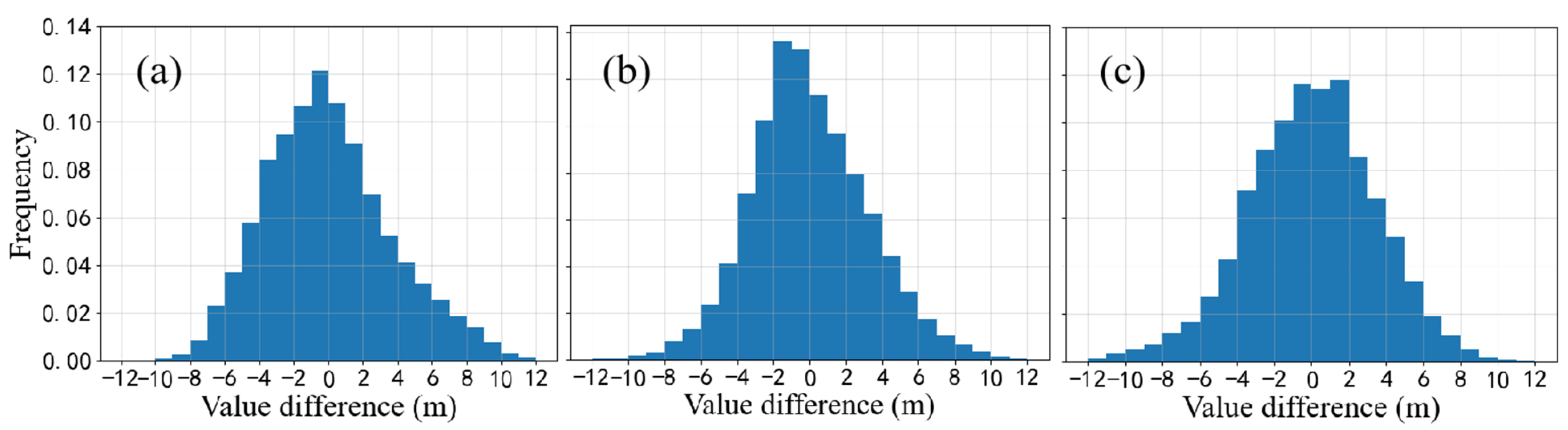
We achieved good inversion results within A1 in Figure 2 by selecting 75% of the data for the experimental set and 25% of the data for the validation set, called Model I. At this point, our training and test sets were placed adjacent to each other, and the training set was kept larger than the test set. Two new sets of experiments were designed to validate the generalization performance of the model. The first set took the first 50% of the data as the training set and the last 25% as the test set to obtain a model called Model II. At this point, the experimental and test regions were separated, and we could observe the effect on model accuracy when the data were adjacent to each other. The second group used 50% of the data as the training set and 50% of the data as the validation set to test the effect of changing the size and proportion of the sample set in the experiment; the resulting model was called Model III. The results of the above three sets of experiments are shown in Table 1. A comparison of the predicted water depth images with the real images is shown in Figure 9; scatter density distribution is shown in Figure 10; and the histogram of the absolute value difference frequency distribution is shown in Figure 11.
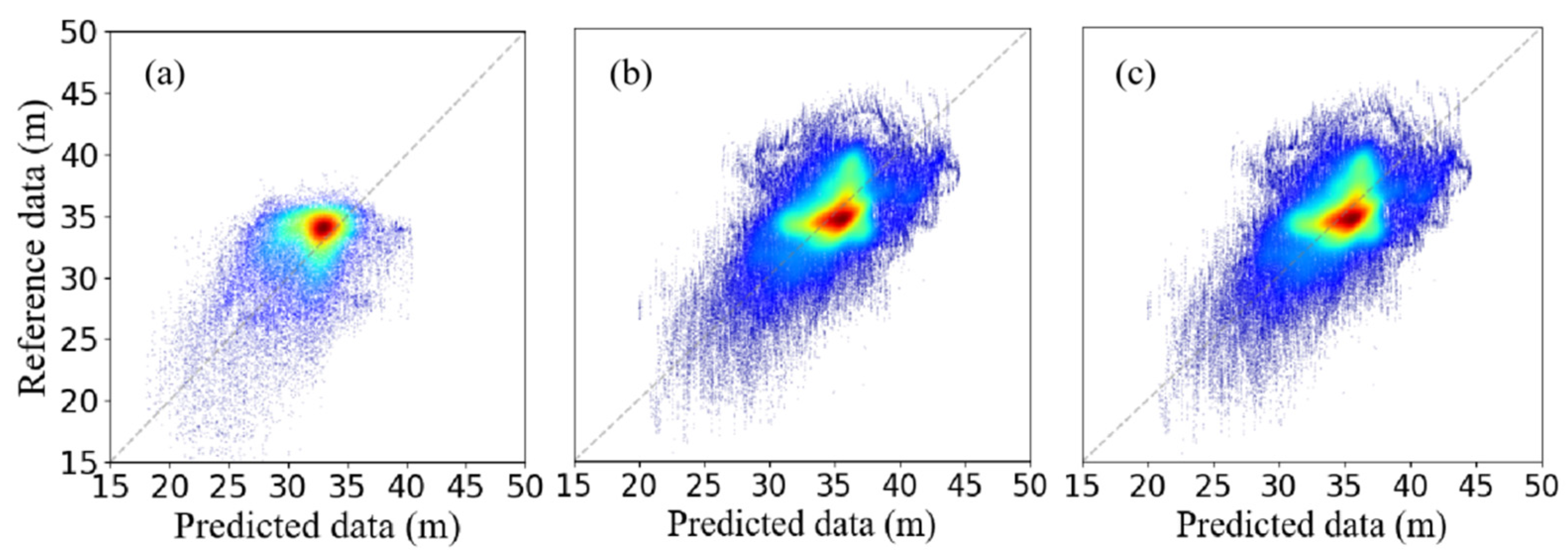
In Figure 9a, the blue line indicates the 50% area boundary, and the green line indicates the 75% boundary. The images in Figure 9b–d indicate that all three sets of models essentially inverted the morphology of the sand wave topography and clearly identified the location of the sand wave crests. Sand wave development was better below the image than that above, and the inversion results were also better below than above. Figure 10 shows a scatter density plot where the horizontal coordinates are the predicted bathymetry values, the vertical coordinates are the measured bathymetry values, and the difference between the horizontal and vertical coordinates at each point represents the prediction error. The scatter points for the three models were distributed roughly along the diagonal, with a higher density closer to the diagonal, indicating a greater number of points with lower deviations. Figure 11 shows a histogram of the different distributions of the three models. The errors of all three models were roughly normally distributed, with a difference of zero, which verified the validity of the models. The accuracy of Model I was slightly higher than that of Models II and III, but the difference was not significant. The scatter distribution pattern of the three sets of experiments was similar, which indicates that the models can be generalized in the area spaced from the training area or in a larger area.
4.2. Model Application
The predicted data from the network were multiplied by the variance plus the mean to obtain the final predicted bathymetry values. The measured bathymetry data in area A1 were obtained using a survey vessel, which facilitated the acquisition of the variance and mean values. Using Model I, predictions were made within areas A2, A3, and A4 in Figure 2. Accuracy validation was performed using the measured line data within the respective regions. We outputted the normalized water depth values using the model.
After the normalized bathymetry had been obtained by inversion, calculating the variance in the bathymetry across the whole area and the regional mean bathymetry was necessary to obtain the specific sand wave bathymetry. Although the sand waves in the Taiwan Banks formed under complex environmental conditions, the sand wave formation conditions in adjacent areas were similar. We used the roughness of bathymetry data in A1 as an approximation for the three validation regions.
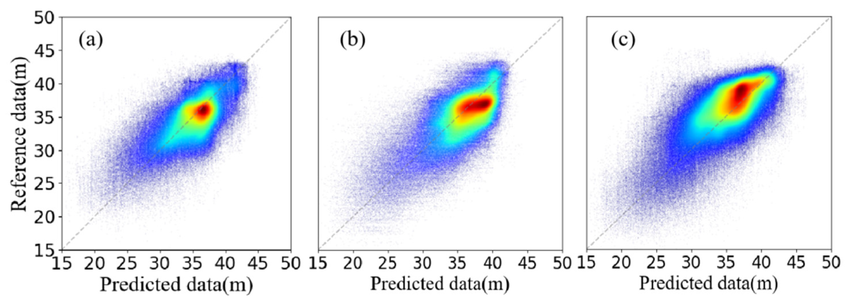
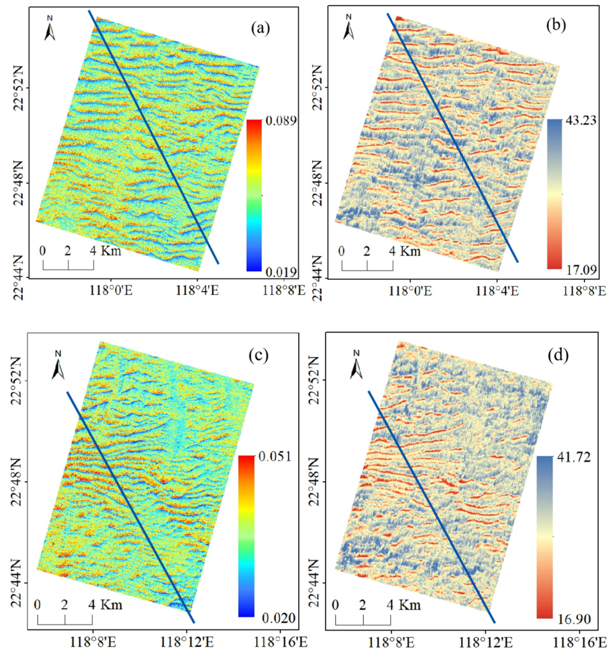
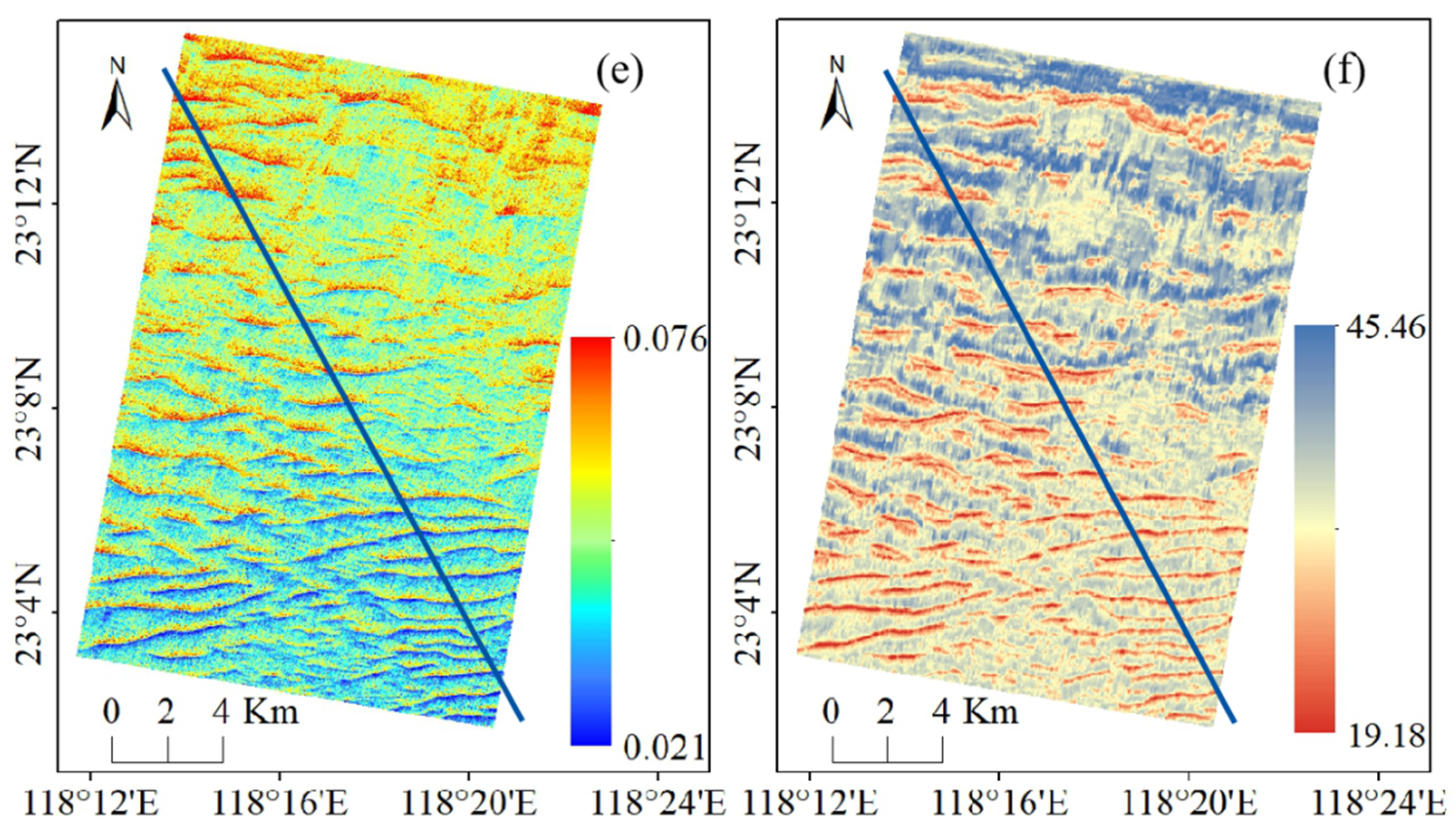
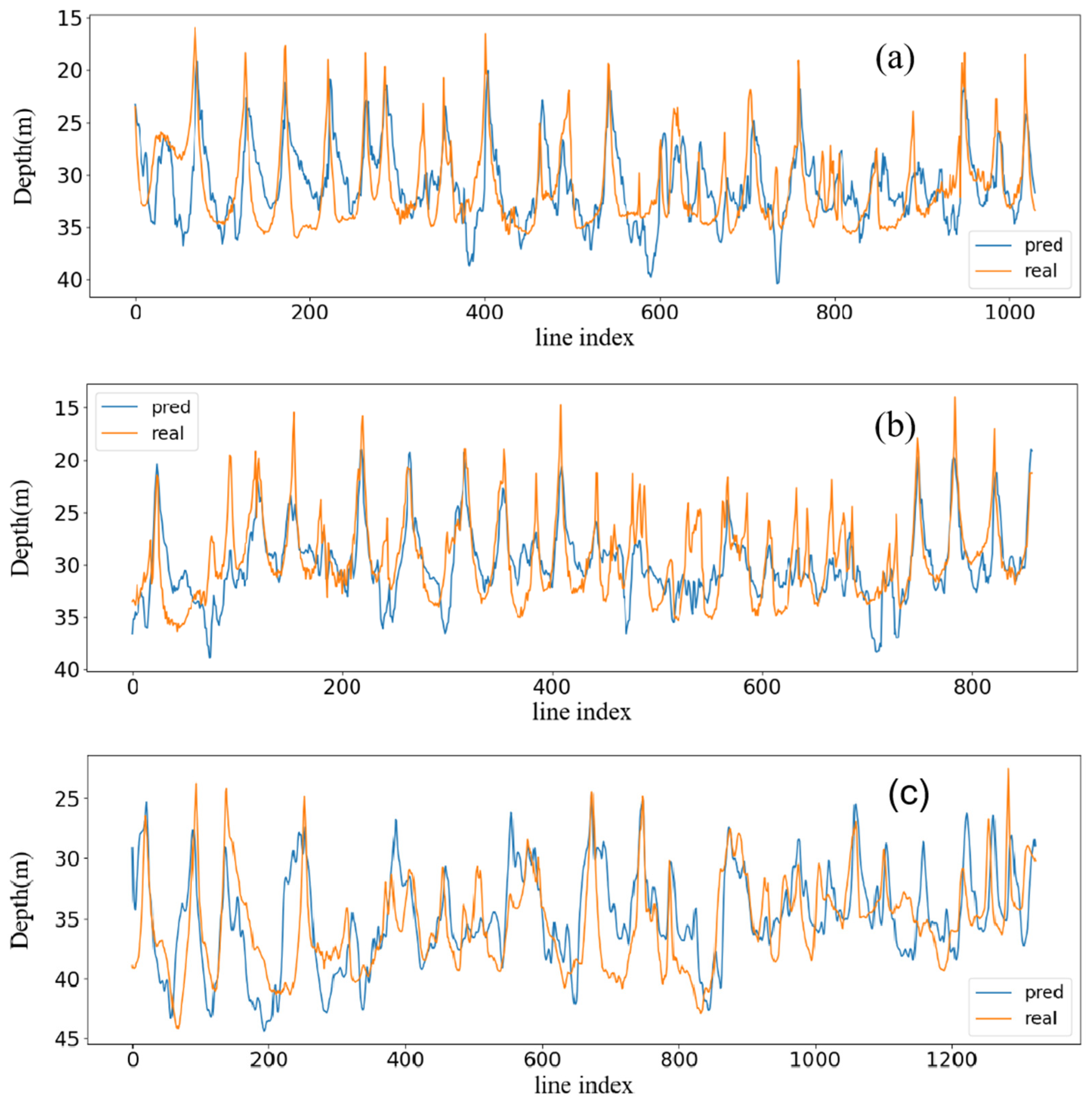
There were 30,000, 60,000, and 130,000 measured bathymetry points on the track lines in areas A2, A3, and A4, respectively, as shown in Figure 2. Although these data points did not cover the entire map, they were representative. The average bathymetry data from the three areas were taken as the average bathymetry of the area. The normalized bathymetry was multiplied by the variance of the bathymetry in area A1, and the mean bathymetry of the survey line was added to obtain the predicted bathymetry. The predicted bathymetry was reduced to a topographic map, as shown in Figure 12. A section of the profile was taken from the measured line in each of the three areas and compared to the predicted bathymetry, as shown in Figure 13. The position of the profile is indicated by the black line in Figure 12. The scatter density distributions of the predicted and measured bathymetry are shown in Figure 14, and the difference distribution is shown in Figure 15. The prediction errors for the three areas are listed in Table 2.
According to Figure 12, on comparing the three sets of roughness images with the inverse bathymetric images, the inversion results reproduced the sand wave pattern. The position of the sand wave crests and of the length and direction of the sand waves were accurately determined. The presence of a trough was due to an impact in the upper right of the A3 area, which is represented by the corresponding position of the inverse bathymetry. Based on the roughness image of area A4, the sand waves were sparse in the upper half of the area and dense in the lower half, with the same effect being seen in the bathymetry image. Though all distinctive sand waves were represented in the inverse bathymetry data, the small and poorly characterized sand waves present in Figure 12c are not present in Figure 12d. The is because the sand waves in this region were shaped too indistinctly to be captured by the model at this time. From Figure 13, the measured and predicted water depths on the three sets of profile lines basically showed the same trend variation. The results of the inversions accurately identified the locations of significant sand wave crests. Although there was a small number of unmatched or incorrectly matched peaks and troughs in all three sets of profiles, and there were some differences between the inverse and real bathymetry values, the overall trend in bathymetry from peak to trough could be reflected.
As indicated by the results in Table 2, the MAE of the inversion results for the three regions ranged from 2.56 to 2.90 m, and the MSE ranged from 3.31 to 3.67 m. As indicated in Figure 14, the predicted and measured values for the three regions were roughly distributed along the diagonal, with an increasing density closer to the diagonal. The difference in values in Figure 15 shows a roughly normal distribution, indicating the validity of the inversion model.
The errors in the inversion results come from three sources: first, the error in the accuracy of the model itself; second, the error caused by the difference between the variance of the water depth in area A1 and in other areas; and third, the error in the mean value of the water depth in the sampled survey line and that in the mean value of the water depth in the whole area. To reduce these errors, the accuracy error of the model itself can be reduced using a higher-accuracy roughness image, or by enhancing the roughness image. It is also possible to improve the representativeness of the sampling to obtain a more accurate mean water depth and to reduce the error introduced by sampling.
5. Discussion
5.1. Errors at Different Depths
As shown in Figure 13, most of the bathymetric profile was a gentle trough. Wave crests were located in areas where bathymetry varied considerably and covered less of the overall location. To investigate the inversion accuracy of the model for different areas, the first 10% of the shallowest water depths were classified as the crest region (<27 m), the deepest 50% (>33 m) were classified as the trough region, and the middle part was termed the transition region (27–33 m). We statistically calculated the errors at different depths within regions A2, A3, and A4, and the results are shown in Table 3.
In all three inversion regions, the error in the wave crest values was significantly higher than that in the other values. There are two reasons for this: first, variance migration has a much greater effect on the peaks and troughs than on the middle part. Second, there was a small number of peaks or troughs that were not matched, and the direct errors in the unmatched peaks and troughs can be greater than 10 m, which significantly increased the errors across the interval. Among the three zones, only the accuracy of the trough data in the A2 zone was higher than the mean value, and the deviations in the positions of the troughs in the other two zones, A3 and A4, were also greater than those in the excess zone. In Figure 12b, several downward peaks from the predicted bathymetry values are evident, and these peaks increased the error in the trough positions. However, because of the wide distribution at trough locations, the sensitivity was lower than that at the crest locations.
5.2. Errors at Different Wavelengths
According to Zhang et al. [8], the wavelength of the sand waves in the Taiwan Banks ranged from 76 to 2151 m, with an average wavelength of 721 m, and their peak occurred at 500 m. We considered sand waves less than 200 m as small sand waves, those between 200 m and 500 m as medium sand waves, and those longer than 500 m as large sand waves. The accuracies at different wavelengths on the oblique survey lines in regions A2, A3, and A4 are listed in Table 4.
The error increased in all regions as the wavelength increased. The reasons for this are two-fold. First, the wavelength of the sand waves is highly correlated with the height of the sand waves. According to the conclusions, higher sand waves resulted in greater errors. Second, larger wavelengths entail more complex structures, such as bimodal sand waves or pendulum sand waves, and the characteristics of the immediately adjacent bimodal peaks make inversion difficult.
5.3. Sensitivity to the Size of the Training Dataset
Neural networks require sufficient training samples. To test the sensitivity of the model to the samples, we used 100%, 75%, 50%, and 25% of region A1 to train the model, and the four groups of trained models were applied to regions A2, A3, and A4. The results are listed in Table 5.
As the size of the training set increased, there was an upward trend in accuracy in the validation region. Using 75% of the training samples, the accuracy was 0.2–0.3 m lower than when using the whole region for training. Each subsequent 25% reduction in training data resulted in a greater error. Therefore, the experimental area needed to be as large as possible; we used the whole A1 area to train the model, and made predictions in the A2, A3, and A4 areas. The experimental dataset was limited to 255 km2, and an increase in the experimental area did not reach the bottleneck of model accuracy. Adding new bathymetric analysis areas to the training set would improve the inversion accuracy.
5.4. Strengths and Weaknesses of the Method
The proposed method is mainly based on SSR for inversion, and remote sensing images with high resolution and high accuracy SSR are available as long as they can be obtained. If an RMSE of 3.31–3.67 m is acceptable for areas without measured water depth data, we can conclude that the proposed LSTM-based inversion method can significantly extend the area of the inversion region. Zhang et al. obtained good results for several sections [8]; however, in their study, the presence of more than two control points located at the crest and trough of the wave on the section was required, and detachment from the control points could not be achieved. He et al. [20] used a joint reconstruction method to achieve the inversion of the water depth; however, accuracy could only be achieved at a maximum of 1 km from the region of measured water depth. Though these data are often used to fill the gaps in multibeam bathymetry data, inversion is not possible in regions without multibeam bathymetry data.
In this study, we proposed the model based on the serial permutation relationship between the results of bathymetry and surface roughness assessment perpendicularly to the sand ridge line. After training on a small amount of measurement data, it can be migrated to other regions for application. For example, in this experiment, bathymetry data of a total sand wave area of 774 km2 were obtained across three areas, A2, A3 and A4. The core feature of this model is the ability to invert large areas without measured bathymetry data with a guaranteed degree of accuracy and the ability to migrate.
The shallow sand wave topography is widely distributed in the tidal environment, and the model proposed herein can be transferred for use in other sand wave areas. However, when transferring the model for other shallow sand wave areas, such as the North Sea in Europe and San Francisco Bay in the USA, local measured water depth data are still required to iterate the model and obtain a locally applicable sand wave sounding model.
6. Conclusions
In this study, LSTM models were introduced to predict the water depth of sand waves, and the following conclusions were obtained.
In this study, a time-series LSTM model was introduced to exploit the continuous, periodic relationship between SSR and bathymetry sequences oriented perpendicularly to the sand waves. The relationship in the spatial domain was mapped to the temporal domain to establish a bathymetric inversion model. The model was designed based on the characteristic relationship between water depth and roughness and has a low dependence on measured water depth data. This addresses the concerns of high cost and small coverage associated with current sun glitter bathymetric inversion models, which rely heavily on the measured water depth data.
The effect of the sea-surface wind field was excluded by experimentally selecting suitable features. The iterative model was trained in the experimental area, and the generalization of the model to non-adjacent areas was verified by changing the experimental area. The model was applied in three non-contiguous areas with a total area of 774 km2, and the accuracy was verified using existing track lines, for which the RMSE was between 3.31 and 3.67 m, and the observed inverse bathymetric images essentially restored the sand wave pattern, enabling the acquisition of low-cost sand wave topography.
The model is based on the relationship between the continuity and periodicity of SSR and sand wave topography and is generalizable in shallow sand wave regions. It can be extended to other areas of sand wave topography, such as the North Sea in Europe, San Francisco Bay in the USA, the South Sea in Korea, and the Bohai Sea and northern South China Sea in China. The model requires a small number of measured bathymetric points to obtain the mean bathymetry of the region, and the reliance on measured bathymetry can be further reduced using other methods to roughly obtain the background bathymetry information for the region.
Author Contributions
Conceptualization, H.Z. and Y.Z.; methodology, Y.Z.; software, Y.Z. and L.Z.; validation, B.F. and Y.Z.; formal analysis, Y.Z. and H.Z.; investigation, H.Z. and B.F.; resources, B.F.; data curation, H.Z.; writing—original draft preparation, Y.Z.; writing—review and editing, H.Z. and L.Z.; visualization, Y.Z.; supervision, L.Z.; project administration, H.Z.; funding acquisition, H.Z. All authors have read and agreed to the published version of the manuscript.
Funding
This research was funded by the National Natural Science Foundation of China (grant numbers 41876208, 41830540, 41576174).
Institutional Review Board Statement
Not applicable.
Informed Consent Statement
Not applicable.
Data Availability Statement
ASTER remote sensing data from publicly available datasets.
Conflicts of Interest
The authors declare no conflict of interest.
References
- McCave, I.N. Sand waves in the North Sea off the coast of Holland. Mar. Geol. 1971, 10, 199–225. [Google Scholar] [CrossRef]
- Park, S.C.; Lee, S.D. Depositional patterns of sand ridges in tide-dominated shallow water environments: Yellow Sea coast and South Sea of Korea. Mar. Geol. 1994, 120, 89–103. [Google Scholar] [CrossRef]
- Barnard, P.L.; Hanes, D.M.; Rubin, D.; Kvitek, R.G. Giant sand waves at the mouth of San Francisco Bay. Eos 2006, 87, 285–289. [Google Scholar] [CrossRef]
- Zhou, J.; Wu, Z.; Jin, X.; Zhao, D.; Cao, Z.; Guan, W. Observations and analysis of giant sand wave fields on the Taiwan Banks, northern South China Sea. Mar. Geol. 2018, 406, 132–141. [Google Scholar] [CrossRef]
- Wang, Y.; Liu, Y.; Jin, S.; Sun, C.; Wei, X. Evolution of the topography of tidal flats and sandbanks along the Jiangsu coast from 1973 to 2016 observed from satellites. ISPRS J. Photogramm. Remote Sens. 2019, 150, 27–43. [Google Scholar] [CrossRef]
- Katoh, K.; Kume, H.; Kuroki, K.; Hasegawa, J. The Development of Sand Waves and the Maintenance of Navigation Channels in the Bisanseto Sea. Coast. Eng. 1999, 1. [Google Scholar] [CrossRef]
- Morelissen, R.; Hulscher, S.J.; Knaapen, M.A.; Németh, A.A.; Bijker, R. Mathematical modelling of sand wave migration and the interaction with pipelines. Coast. Eng. 2003, 48, 197–209. [Google Scholar] [CrossRef]
- Zhang, H.G.; Yang, K.; Lou, X.L.; Li, D.L.; Shi, A.Q.; Fu, B. Bathymetric mapping of submarine sand waves using multi-angle sun glitter imagery: A case of the Taiwan Banks with ASTER stereo imagery. J. Appl. Remote Sens. 2015, 9, 095988-1–095988-13. [Google Scholar] [CrossRef] [Green Version]
- Lee, Z.; Hu, C.; Casey, B.; Shang, S.; Dierssen, H.; Arnone, R. Global Shallow-Water Bathymetry From Satellite Ocean Color Data. Eos 2010, 91, 429–430. [Google Scholar] [CrossRef] [Green Version]
- Fan, K. Remote sensing of SAR shallow sea topography based on sea surface microwave scattering imaging. Acta Geod. Cartogr. Sin. 2010, 39, 329. [Google Scholar]
- Liu, Z.C.; Zhou, X.H.; Chen, Y.L.; Hu, G.H. The development in the latest technique of shallow water multi-beam sounding system. Hydrogr. Surv. Charting 2005, 6, 21. [Google Scholar]
- Catalao, J.; Nico, G. Multitemporal Backscattering Logistic Analysis for Intertidal Bathymetry. IEEE Trans. Geosci. Remote Sens. 2017, 55, 1066–1073. [Google Scholar] [CrossRef]
- Alpers, W.; Hennings, I. A theory of the imaging mechanism of underwater bottom topography by real and synthetic aperture radar. J. Geophys. Res. Space Phys. 1984, 89, 10529–10546. [Google Scholar] [CrossRef]
- Calkoen, C.J.; Hesselmans, G.; Wensink, G.J.; Vogelzang, J. The bathymetry assessment system: Efficient depth mapping in shallow seas using radar images. Int. J. Remote Sens. 2001, 22, 29732998. [Google Scholar] [CrossRef]
- Weigen, H.; Bin, F. A spaceborne SAR technique for shallow water bathymetry surveys. J. Coastal Res. 2004, 43, 223–228. [Google Scholar]
- Hennings, I.; Doerffer, R.; Alpers, W. Comparison of submarine relief features on a radar satellite image and on a Skylab satellite photograph. Int. J. Remote Sens. 1988, 9, 45–67. [Google Scholar] [CrossRef]
- Cox, C.; Munk, W. Measurement of the Roughness of the Sea Surface from Photographs of the Sun’s Glitter. J. Opt. Soc. Am. 1954, 44, 838–850. [Google Scholar] [CrossRef]
- Hennings, I.; Matthews, J.; Metzner, M. Sun glitter radiance and radar cross-section modulations of the sea bed. J. Geophys. Res. Space Phys. 1994, 99, 16303–16326. [Google Scholar] [CrossRef]
- Shao, H.; Li, Y.; Li, L. Sun glitter imaging of submarine sand waves on the Taiwan Banks: Determination of the relaxation rate of short waves. J. Geophys. Res. Space Phys. 2011, 116, 06024. [Google Scholar] [CrossRef] [Green Version]
- He, X.; Chen, N.; Zhang, H.; Fu, B.; Wang, X. Reconstruction of sand wave bathymetry using both satellite imagery and multi-beam bathymetric data: A case study of the Taiwan Banks. Int. J. Remote Sens. 2014, 35, 3286–3299. [Google Scholar] [CrossRef]
- Liu, S.; Wang, L.; Liu, H.; Su, H.; Li, X.; Zheng, W. Deriving Bathymetry from Optical Images with a Localized Neural Network Algorithm. IEEE Trans. Geosci. Remote Sens. 2018, 56, 5334–5342. [Google Scholar] [CrossRef]
- Alevizos, E. A Combined Machine Learning and Residual Analysis Approach for Improved Retrieval of Shallow Bathymetry from Hyperspectral Imagery and Sparse Ground Truth Data. Remote Sens. 2020, 12, 3489. [Google Scholar] [CrossRef]
- Panagiotis, A.; Konstantinos, K.; Georgopoulos, A.; Skarlatos, D. Correcting image refraction: Towards accurate aerial image-based bathymetry mapping in shallow waters. Remote Sens. 2020, 12, 322. [Google Scholar]
- Xiaorun, L.; Li, X.; Zhang, H.; Wang, J.; Lou, X.; Fan, K.; Shi, A.; Li, D. A Bathymetry Mapping Approach Combining Log-Ratio and Semianalytical Models Using Four-Band Multispectral Imagery Without Ground Data. IEEE Trans. Geosci. Remote Sens. 2020, 58, 2695–2709. [Google Scholar] [CrossRef]
- Sepp, H.; Schmidhuber, J. Unsupervised coding with lococode. In Proceedings of the Artificial Neural Networks—ICANN’97, Lausanne, Switzerland, 8–10 October 1997; pp. 655–660. [Google Scholar]
- Fang, K.; Pan, M.; Shen, C. The Value of SMAP for Long-Term Soil Moisture Estimation with the Help of Deep Learning. IEEE Trans. Geosci. Remote Sens. 2018, 57, 2221–2233. [Google Scholar] [CrossRef]
- Xu, L.; Li, Q.; Yu, J.; Wang, L.; Xie, J.; Shi, S. Spatio-temporal predictions of SST time series in China’s offshore waters using a regional convolution long short-term memory (RC-LSTM) network. Int. J. Remote Sens. 2020, 41, 3368–3389. [Google Scholar] [CrossRef]
- Wang, F.; Chen, Y.; Li, Z.; Fang, G.; Li, Y.; Wang, X.; Zhang, X.; Kayumba, P. Developing a Long Short-Term Memory (LSTM)-Based Model for Reconstructing Terrestrial Water Storage Variations from 1982 to 2016 in the Tarim River Basin, Northwest China. Remote Sens. 2021, 13, 889. [Google Scholar] [CrossRef]
- Zhang, L.; Zhang, Z.; Luo, Y.; Cao, J.; Tao, F. Combining Optical, Fluorescence, Thermal Satellite, and Environmental Data to Predict County-Level Maize Yield in China Using Machine Learning Approaches. Remote Sens. 2019, 12, 21. [Google Scholar] [CrossRef] [Green Version]
- Yu, W.; Wu, Z.Y.; Zhou, J.Q.; Zhao, D.N. Meticulous characteristics, classification and distribution of seabed sand wave on the Taiwan bank. Haiyang Xuebao 2015, 37, 11–25. [Google Scholar]
- Bao, J.; Cai, F.; Shi, F.; Wu, C.; Zheng, Y.; Lu, H.; Sun, L. Morphodynamic response of sand waves in the Taiwan Shoal to a passing tropical storm. Mar. Geol. 2020, 426, 106196. [Google Scholar] [CrossRef]
- Zhang, H.; Yang, K.; Lou, X.; Li, Y.; Zheng, G.; Wang, J.; Wang, X.; Ren, L.; Li, D.; Shi, A. Observation of sea surface roughness at a pixel scale using multi-angle sun glitter images acquired by the ASTER sensor. Remote Sens. Environ. 2018, 208, 97–108. [Google Scholar] [CrossRef]
- Wang, Z. Text emotion detection based on Bi- LSTM network. J. Inf. Comput. Sci. 2020, 3, 129–137. [Google Scholar]
- Karevan, Z.; Suykens, J.A. Transductive LSTM for time-series prediction: An application to weather forecasting. Neural Netw. 2020, 125, 1–9. [Google Scholar] [CrossRef] [PubMed]
- Schmidhuber, J. Deep learning in neural networks: An overview. Neural Netw. 2015, 61, 85–117. [Google Scholar] [CrossRef] [Green Version]
- Wang, X.; Liu, M.; Guan, Y. Image edge detection algorithm based on improved canny operator. Comp. Eng. 2012, 38, 196–198. [Google Scholar]
Figure 1.
Taiwan Strait shallow sand wave topography in full view. The red boundary indicates the outer envelope range of the shallow Taiwan Strait with an area of ~16,400 km2, and the black box indicates the remote sensing image range as in Figure 2 with an area of ~3600 km2.
Figure 1.
Taiwan Strait shallow sand wave topography in full view. The red boundary indicates the outer envelope range of the shallow Taiwan Strait with an area of ~16,400 km2, and the black box indicates the remote sensing image range as in Figure 2 with an area of ~3600 km2.

Figure 2.
(a) Experimental area of A1, A2, A3, and A4. The purple line is the measured water depth in 2012, and the blue line is the measured water depth in 2017. The legend indicates the value of the SSR. (b) Distribution of 25 measurement lines with 500 m interval in A1 area.
Figure 2.
(a) Experimental area of A1, A2, A3, and A4. The purple line is the measured water depth in 2012, and the blue line is the measured water depth in 2017. The legend indicates the value of the SSR. (b) Distribution of 25 measurement lines with 500 m interval in A1 area.

Figure 3.
(a) Water depth in area A1 obtained by interpolating with 500 m interval bathymetric lines, (b) roughness in area A1, (c) variations in water depth on the profile line, (d) variations in SSR on the profile line.
Figure 3.
(a) Water depth in area A1 obtained by interpolating with 500 m interval bathymetric lines, (b) roughness in area A1, (c) variations in water depth on the profile line, (d) variations in SSR on the profile line.

Figure 4.
Experimental flow. Slanted boxes indicate input data, straight boxes indicate actions, rounded boxes indicate output data, and arrows indicate sequence.
Figure 4.
Experimental flow. Slanted boxes indicate input data, straight boxes indicate actions, rounded boxes indicate output data, and arrows indicate sequence.

Figure 5.
(a) Cross-filtered template and (b) original SSR on the profile line and filtered SSR.

Figure 6.
Node structure of the LSTM.
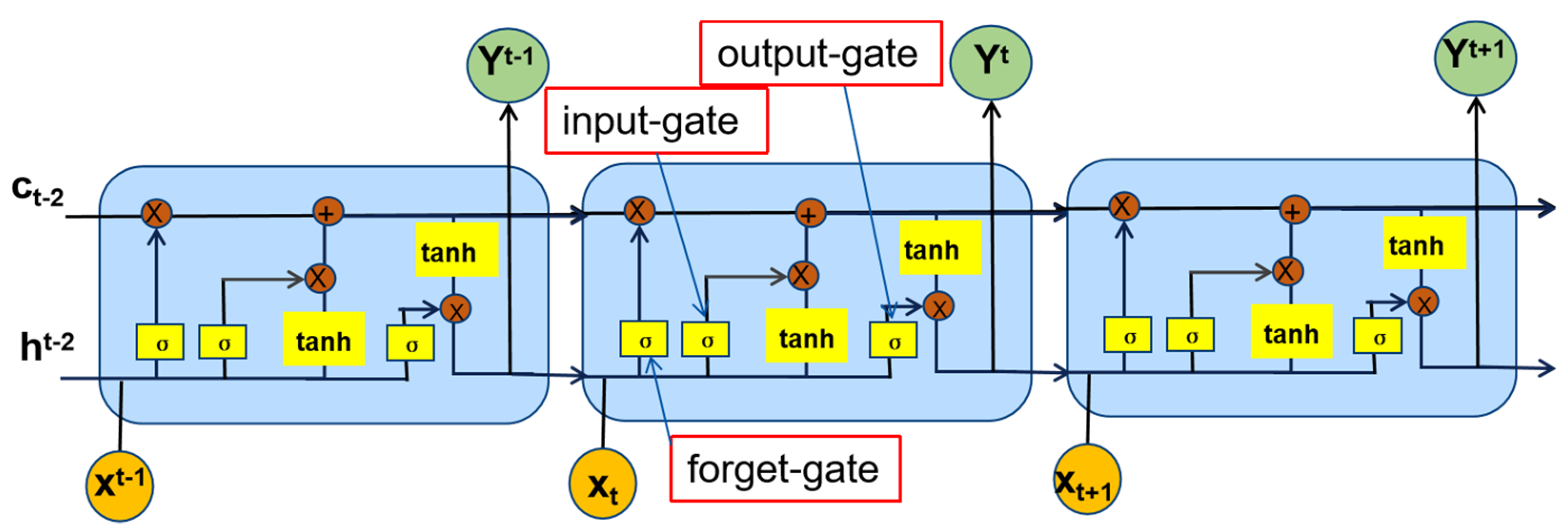
Figure 7.
LSTM neural network topology.
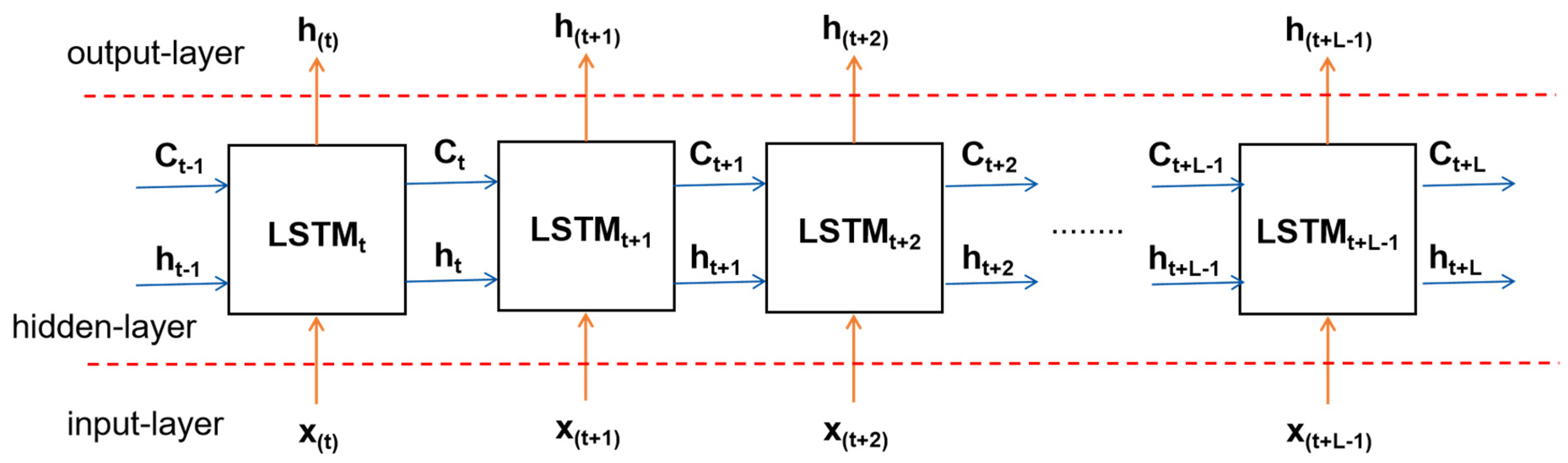
Figure 8.
Train loss and test loss variation.

Figure 9.
(a) Water depth in region A1 obtained by interpolating with 500 m interval bathymetric lines. The blue line and green line indicate the 50% and 75% demarcation lines of the A1 region, respectively, (b) predicted water depth obtained from Model I, (c) predicted water depth obtained from Model II, and (d) predicted water depth obtained from Model III.
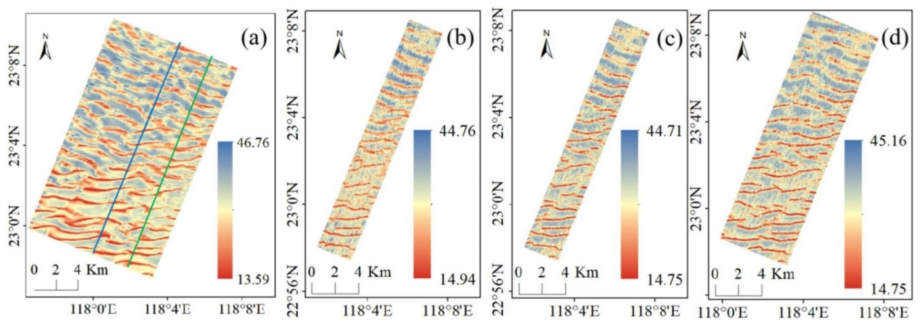
Figure 10.
Scatter density distribution of predicted water depths for (a) Model I, (b) Model II, and (c) Model III.
Figure 10.
Scatter density distribution of predicted water depths for (a) Model I, (b) Model II, and (c) Model III.

Figure 11.
Histograms of the difference frequency distribution of predicted water depths for (a) Model I, (b) Model II, and (c) Model III.
Figure 11.
Histograms of the difference frequency distribution of predicted water depths for (a) Model I, (b) Model II, and (c) Model III.
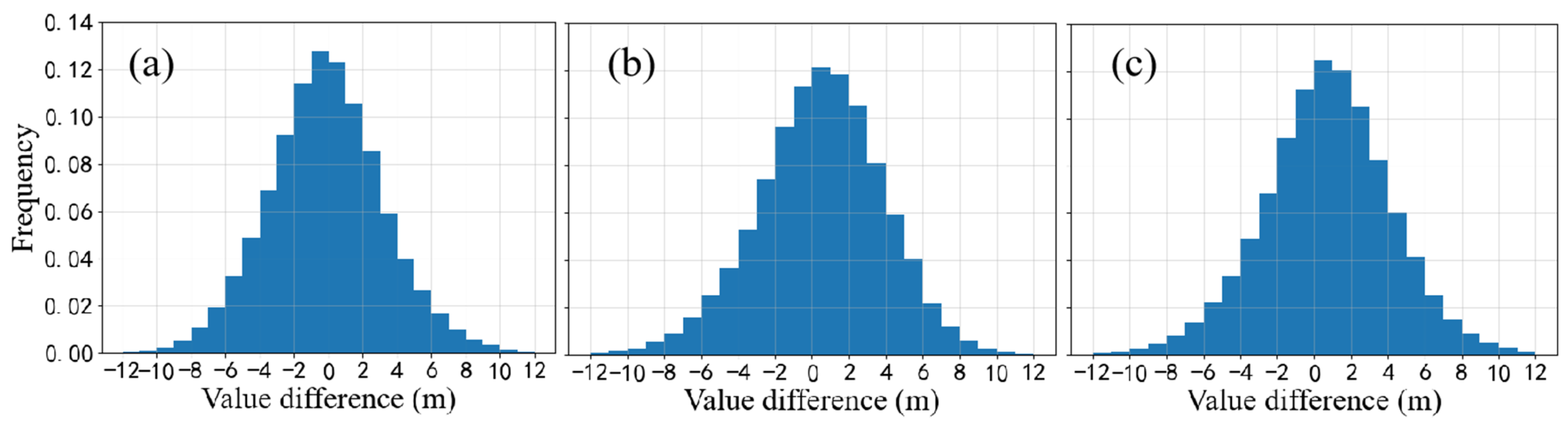
Figure 12.
(a) Roughness of area A2, (b) predicted water depth of area A2, (c) roughness of area A3, (d) predicted water depth of area A3, (e) roughness of area A4, (f) predicted water depth of area A4. Blue lines indicate measured profile lines.
Figure 12.
(a) Roughness of area A2, (b) predicted water depth of area A2, (c) roughness of area A3, (d) predicted water depth of area A3, (e) roughness of area A4, (f) predicted water depth of area A4. Blue lines indicate measured profile lines.


Figure 13.
Sections of areas (a) A2, (b) A3, and (c) A4.

Figure 14.
Scatter density plots of predicted water depths in areas (a) A2, (b) A3, and (c) A4.

Figure 15.
Difference distribution of predicted water depths in areas (a) A2, (b) A3, and (c) A4.

Table 1.
Presentation of model results.
| Model I | Model II | Model III | |
|---|---|---|---|
| Mean absolute error (m) | 2.63 | 2.72 | 2.79 |
| Root mean square error (m) | 3.36 | 3.45 | 3.59 |
Table 2.
Accuracy of predicted water depths within areas: A2, A3, and A4.
| Region A2 | Region A3 | Region A4 | |
|---|---|---|---|
| Mean absolute error (m) | 2.90 | 2.56 | 2.73 |
| Root mean square error (m) | 3.67 | 3.31 | 3.46 |
| Area size (km2) | 224 | 202 | 348 |
Table 3.
Error analysis for different depths in the three regions.
| Inversion Region | RMSE (m) at Different Depths | |||
|---|---|---|---|---|
| <27 m | 27–33 m | >33 m | Total | |
| A2 | 5.00 | 3.55 | 3.28 | 3.67 |
| A3 | 4.14 | 2.57 | 3.88 | 3.31 |
| A4 | 4.55 | 3.36 | 3.41 | 3.46 |
| Total | 4.42 | 3.10 | 3.47 | |
Table 4.
Verification of the accuracy of sand wave depth at different wavelengths.
| Inversion Region | RMSE (m) at Different Wavelengths | |||
|---|---|---|---|---|
| <200 m | 200–500 m | >500 m | Total | |
| A2 | 3.13 | 4.24 | 5.10 | 3.67 |
| A3 | 3.19 | 3.22 | 3.58 | 3.31 |
| A4 | 3.26 | 3.28 | 4.41 | 3.46 |
| Total | 3.18 | 3.62 | 4.46 | |
Table 5.
Validation accuracy of regions A2, A3, and A4 for different training set sizes.
| Inversion Region | Accuracy under Differently Sized Training Sets RMSE (m) | |||
|---|---|---|---|---|
| Region A1 | 75% of Region A1 | 50% of Region A1 | 25% of Region A1 | |
| Size (km2) | 255 | 192 | 128 | 64 |
| A2 | 3.67 | 3.89 | 4.55 | 5.01 |
| A3 | 3.31 | 3.52 | 4.10 | 4.71 |
| A4 | 3.46 | 3.72 | 3.91 | 4.45 |
Publisher’s Note: MDPI stays neutral with regard to jurisdictional claims in published maps and institutional affiliations. |
© 2021 by the authors. Licensee MDPI, Basel, Switzerland. This article is an open access article distributed under the terms and conditions of the Creative Commons Attribution (CC BY) license (https://creativecommons.org/licenses/by/4.0/).
Share and Cite
MDPI and ACS Style
Zhao, Y.; Zhao, L.; Zhang, H.; Fu, B. LSTM-Based Remote Sensing Inversion of Largescale Sand Wave Topography of the Taiwan Banks. Remote Sens. 2021, 13, 3313. https://0-doi-org.brum.beds.ac.uk/10.3390/rs13163313
AMA Style
Zhao Y, Zhao L, Zhang H, Fu B. LSTM-Based Remote Sensing Inversion of Largescale Sand Wave Topography of the Taiwan Banks. Remote Sensing. 2021; 13(16):3313. https://0-doi-org.brum.beds.ac.uk/10.3390/rs13163313
Chicago/Turabian StyleZhao, Yujin, Liaoying Zhao, Huaguo Zhang, and Bin Fu. 2021. "LSTM-Based Remote Sensing Inversion of Largescale Sand Wave Topography of the Taiwan Banks" Remote Sensing 13, no. 16: 3313. https://0-doi-org.brum.beds.ac.uk/10.3390/rs13163313
Note that from the first issue of 2016, this journal uses article numbers instead of page numbers. See further details here.