
Field Observations of Breaking of Dominant Surface Waves
by
 , ,
, ,
Pavel D. Pivaev
1,2,* ,
,
Vladimir N. Kudryavtsev
1,2,
Aleksandr E. Korinenko
2 and
Vladimir V. Malinovsky
2 1
Satellite Oceanography Laboratory, Russian State Hydrometeorological University, 98 Malookhtinskiy Av., 195196 St-Petersburg, Russia
2
Remote Sensing Department, Marine Hydrophysical Institute of RAS, 2 Kapitanskaya St., 299011 Sevastopol, Russia
*
Author to whom correspondence should be addressed.
Remote Sens. 2021, 13(16), 3321; https://0-doi-org.brum.beds.ac.uk/10.3390/rs13163321
Submission received: 12 July 2021
/
Revised: 17 August 2021
/
Accepted: 19 August 2021
/
Published: 22 August 2021
(This article belongs to the Special Issue Passive Remote Sensing of Oceanic Whitecaps)
Abstract
:The results of field observations of breaking of surface spectral peak waves, taken from an oceanographic research platform, are presented. Whitecaps generated by breaking surface waves were detected using video recordings of the sea surface, accompanied by co-located measurements of waves and wind velocity. Whitecaps were separated according to the speed of their movement, c, and then described in terms of spectral distributions of their areas and lengths over c. The contribution of dominant waves to the whitecap coverage varies with the wave age and attains more than 50% when seas are young. As found, the whitecap coverage and the total length of whitecaps generated by dominant waves exhibit strong dependence on the dominant wave steepness, , the former being proportional to . This result supports a parameterization of the dissipation term, used in the WAM model. A semi-empirical model of the whitecap coverage, where contributions of breaking of dominant and equilibrium range waves are separated, is suggested.
1. Introduction
The breaking of ocean surface waves has been a subject of extensive scientific investigations over the past decades, and significant progress in understanding of underlying physics and statistical properties of breaking waves has already been made [1,2,3,4]. Wave breaking is the principal mechanism of wave energy dissipation playing a crucial role in the energy balance of surface waves. Form drag, supported by the airflow separation from breaking crests, sea spray, and turbulence generated by breaking waves beneath the surface are important agents in momentum, heat and gas exchanges at the ocean surface [5,6,7,8,9,10].
In the context of remote sensing, wave breaking contributes significantly to the intensity of the radar backscatter at any polarization configuration [11,12,13,14] as well as to the Doppler shift (see, e.g., [15] and references cited therein). Radar returns from breaking waves can apparently result in overestimation of the sea surface height derived from space-born altimeters [16], thereby forming a part of a so-called sea state bias in altimeter data [17,18,19]. Dielectric properties of foam produced by breaking waves differ from those of water and notably affect surface microwave emissivity, which is necessary to take into account in processing and interpretation of the measurements made by space-born passive microwave instruments [20,21,22]. Availability and extensive use of satellite microwave data in L-band had led to comprehension that breaking of large-scale waves produces the thickest foam that can significantly impact measurements of passive microwave instruments in this frequency band [23,24].
The breaking of dominant waves (spectral peak waves) deserves special attention. Dominant waves contain most of the energy of the sea surface. Developing under extreme atmospheric synoptic-scale systems, they can attain abnormal heights, representing a serious threat to an open-sea navigation and coastal areas [25,26]. Therefore, modelling of the evolution of such waves, especially under severe wind conditions, is an issue of high priority. Amongst energy sources governing spectral peak dynamics—nonlinear wave-wave interactions, wind energy input and wave breaking dissipation—the latter is the only term whose exact form remains unknown, and, as a consequence, various parametrisations based on different physical approaches were suggested (see [4] and Section II.4 in [27]). Effectively, the description of wave breaking dissipation, for the time being, has a semi-empirical character. Typically, the dissipation term serves as a fitting function providing consistency between wave model simulations and observational data (see, e.g., Chapter 2.3 in [28]). In this regard, the development of the realistic and physically grounded description of dominant wave breaking is very desirable and valuable both for wave modelling and microwave remote sensing methods.
Most of the studies on wave breaking hitherto have limited their attention to equilibrium range waves. Field observations of breaking of spectral peak waves are rare, and all have focused on a breaking probability. The authors in [29,30,31,32] reported estimates of the dominant wave breaking probability that were based on counting of breaking events either using visual inspection, acoustic noise or water conductivity measurements.
The aim of the present study is to investigate whitecaps generated by breaking of spectral peak waves and relationships between properties of the whitecaps and wind speed, as well as properties of dominant waves, using video imagery of the sea surface in the visible range. Discrimination between whitecaps produced by dominant and shorter wind-waves is carried out according to the speed of advance of the whitecaps, i.e., following an approach suggested by O. Phillips [33].
In Section 2, we describe the experimental equipment, data processing methods, estimated parameters, and the selection of measurement time intervals. Results are presented in Section 3. In Section 4, we suggest a semi-empirical model of the whitecap coverage, where the distinction between breaking of dominant and equilibrium range waves is made. A summary of the main findings is given in Section 5.
2. Materials and Methods
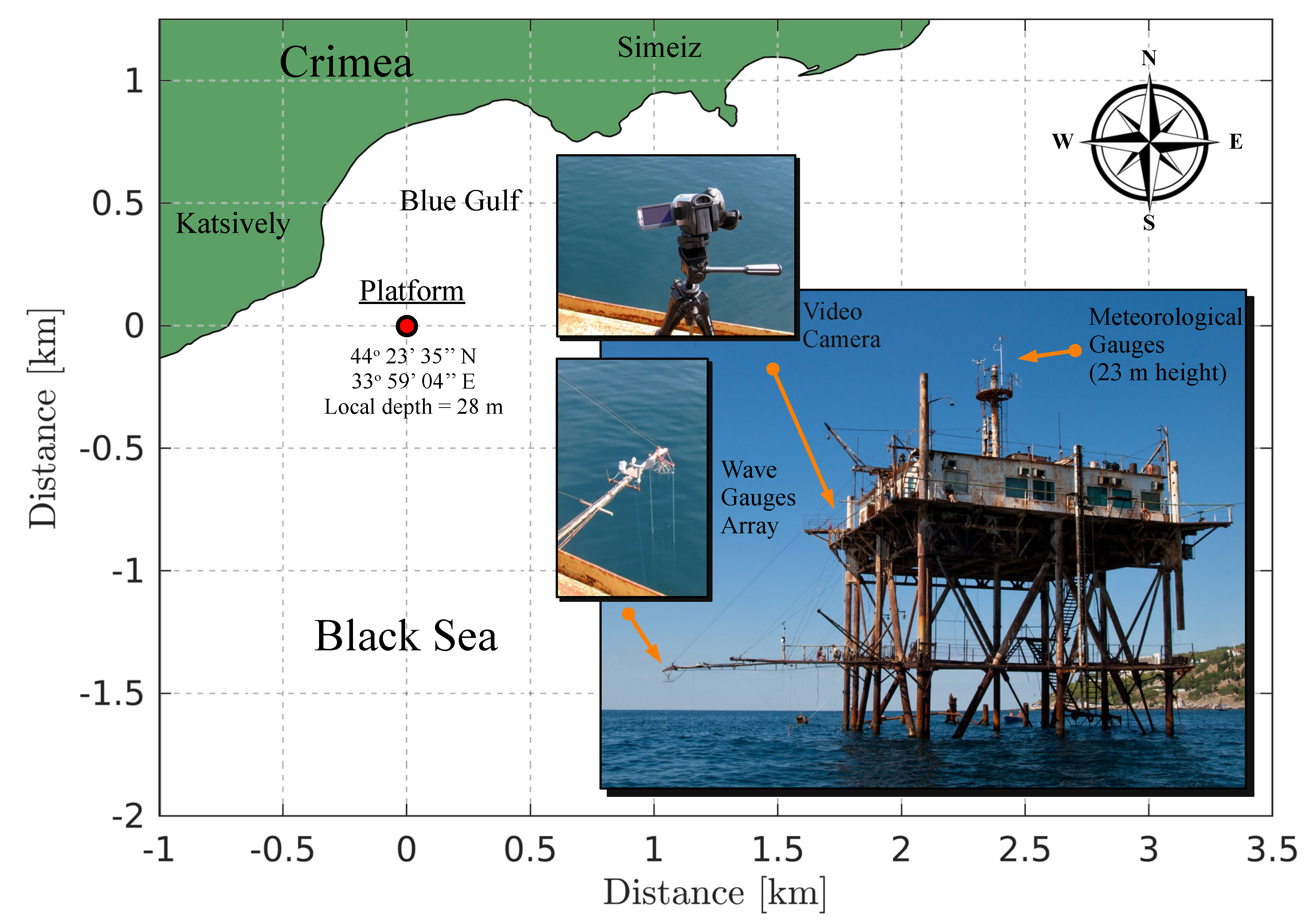
The data considered in this study were collected during autumn experimental campaigns in 2013–2015, 2018 and 2019 on a Black Sea research platform located 400 m away from the coast, near Katsively settlement, Crimea (see Figure 1). Below we provide a brief overview of instrumentation. The reader is referred to [34,35] for a more detailed description.
2.1. Experimental Equipment
Elevations of the sea surface were measured by an array of wave gauges operating at 20 Hz sampling frequency. The array consisted of six resistance string gauges distributed over the vertices of a regular pentagon (plus an additional string in the centre) with the circumradius of 25 cm. In 2018, owing to technical issues, only a single-string wave gauge, operating at 10 Hz sampling frequency, was used.
The wind speed, its direction, air temperature and relative humidity were measured by a meteorological weather station mounted at 23 m height above the sea surface. Using additional measurements of the water temperature, we applied the COARE algorithm [36] to convert the wind speed to a standard 10 m height.
A video camera - was used to make video recordings of the sea surface. The camera was mounted on a tripod and fasted to the platform’s base at 11.4 m height above the sea level. The incidence angles of the camera varied in the range 50–65, and the viewing angles of the lens were along horizontal and along vertical. At such viewing geometry, the spatial resolution varied from about 1 cm to 2.5 cm. Sequences of images were taken at a 50 frames per second rate with a 1920 × 1080 pixels resolution. The observable surface area ranged from 311 to 2700 m.
2.2. Wave and Wave Breaking Parameters
Owing to the specific location of the platform, observed sea states ranged from very young to mature seas. Young wind-waves with inverse wave ages, ( is the wind speed at 10 m reference height, is the spectral peak phase speed), up to 6 were generated by north winds associated with rather short, less than 1 km, fetches (see Figure 1). Henceforth, we shall refer to these cases as the - ones. In all of these cases, developing wind-waves were superimposed on open-sea swell. For east and south-east winds, wind-waves, reaching the platform, could be characterised as mature with inverse wave ages of about 2. These sea conditions will be referred to as - cases.
2.2.1. Waves
Surface elevation frequency spectra, , were routinely derived from a single wave gauge using a conventional technique [37]. Additionally, directional spectra, , were also estimated using the Extended Maximum Entropy Principle method [38], freely available code being used [39].
In most cases, seas at the experimental site could be considered as mixed ones, i.e., wave fields were the superposition of developing wind-waves and swell. To discriminate the two types of wave systems, we used a method suggested by [40], according to which swell was defined as a part of the frequency spectrum lying below Toba’s equilibrium range level [41].
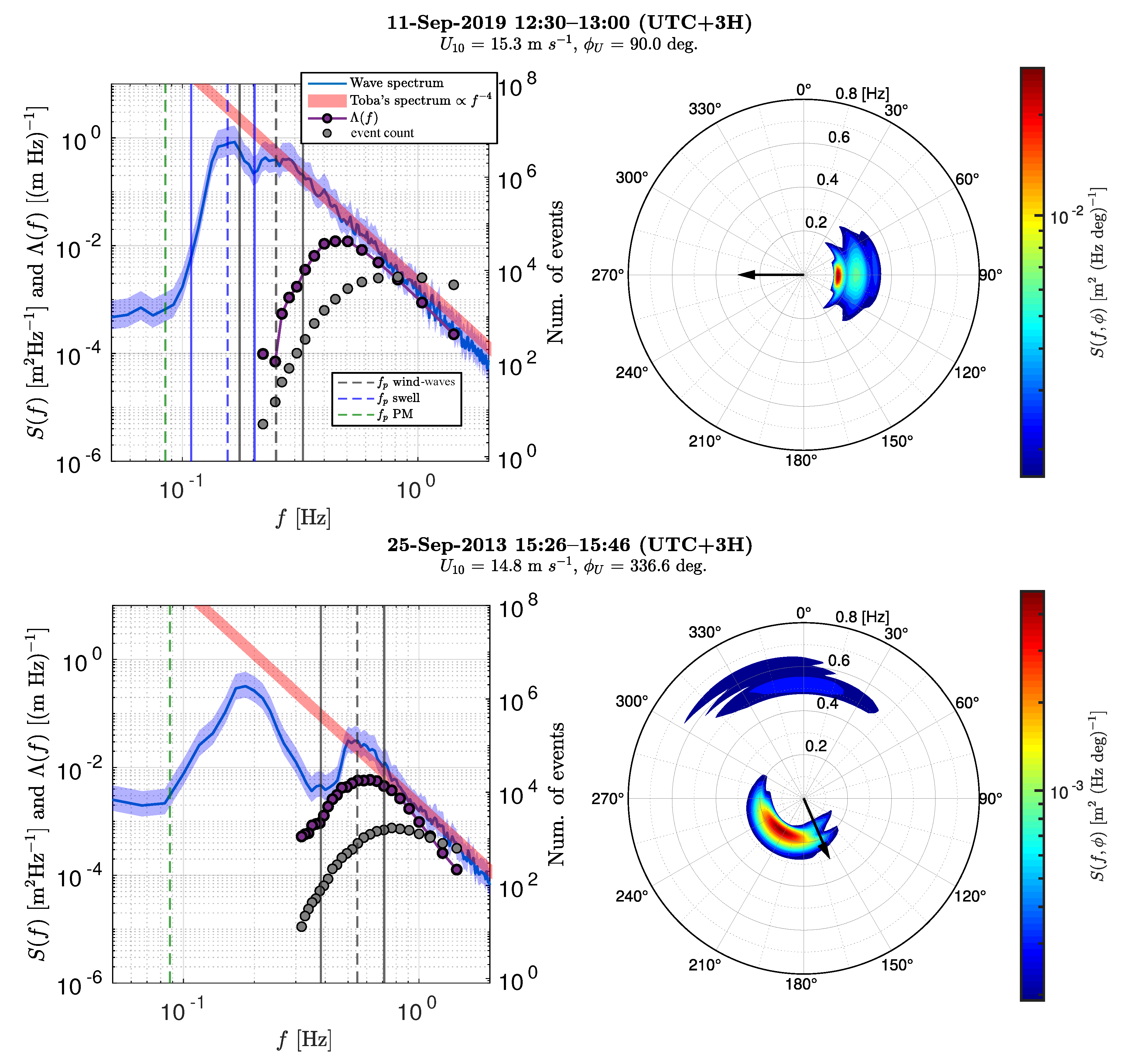
Examples of frequency and directional wave spectra are shown in Figure 2, where the Pierson-Moskowitz frequency [42] is displayed to indicate fully developed waves. On 11 September 2019, spectral peaks of wind-waves and swell are not well separated, but clearly distinguishable. The corresponding directional wave spectrum shows that these wave systems propagate in the same along-wind direction. Coexisting wind-waves and swell in all of the onshore-wind conditions were not well separated both in directional and frequency spectra. On 25 September 2013, the typical offshore-wind case, considerable split between wind-waves and swell in frequency as well as direction domains can be seen.
We quantify dominant waves in terms of the spectral peak frequency, , and variance, (referred to as energy). In the case of mixed seas in the onshore-wind conditions, of wind-waves was determined as the low-frequency intersection of Toba’s equilibrium range spectrum with the measured . In the offshore-wind conditions, of wind-waves was assigned manually. Following [30,31,32], the energy of dominant waves is defined as the variance of surface elevations in the frequency band , where [43]:
If spectral peak frequency bands of swell and wind-waves overlap with one another, the integration domain in (1) can be “contaminated” with the energy of swell, as seen from Figure 2. As mentioned above, mixed seas in the onshore-wind conditions demonstrated poorly separated wind and swell wave systems both in frequency and direction domains. To mitigate the energy contamination effect, we implemented one-dimensional spectrum partitioning procedure described in Appendix A. After the procedure was applied, the energy of dominant wind-waves was estimated according to (1).
Other important wave parameters, inferred from and , are the inverse wave age, , and the dominant wave steepness [30], (, and is the spectral peak wavenumber). The peak frequency and wavenumber are related to one another via the deep water dispersion relationship of surface gravity waves
where is the angular wave frequency, g is the gravitational acceleration. Additionally, the propagation direction of dominant waves, , was determined as the direction of the maximum of .
2.2.2. Wave Breaking
Phillips [33] introduced a convenient measure to describe breaking waves such that is the sum of lengths of breaking crests moving with speeds in range per unit surface area. The total length of breaking crests of all waves per unit surface area is then,
Similar to the definition of , we introduce an active whitecap coverage distribution, , such that represents the fraction of the sea surface covered by whitecaps that move with speeds in range (). The total active whitecap coverage is therefore
A relationship between the phase speed of the breaking wave and the speed of the corresponding breaking crest (or the whitecap) is still an issue. Laboratory investigations [44,45,46] revealed that the speed of advance of the breaking crest, c, is slightly less than the phase speed of the underlying wave, , i.e., , where . Validity of these estimates in real conditions has not been established experimentally. In this work, we assume a neutral relationship.
In order to extract geometric and kinematic properties of individual breaking crests from video recordings, an algorithm devised by Mironov and Dulov [47] was employed. It is important to note that the algorithm aims to detect —active whitecaps, if we adopt terminology from [48] (“stage A” breaking [49] or “dynamic foam” [23,50])—and effectively disregards residual foam and bubble wakes (“stage B” breaking [49] or “static foam” [23,50]) produced by breaking crests.
The optical parameters of the camera were obtained using an open-source camera calibration toolbox [51]. These parameters allowed orthorectification of the original images of the sea surface. Distortion effects due to the camera’s lens were ignored. As was estimated, the error associated with this type of distortion in measuring the whitecap lengths did not exceed 10% for the data on 24 September 2013. This day is characterized by the largest incidence angles of the camera. On other days, the incidence angles were significantly smaller, therefore the error was less than 10%.
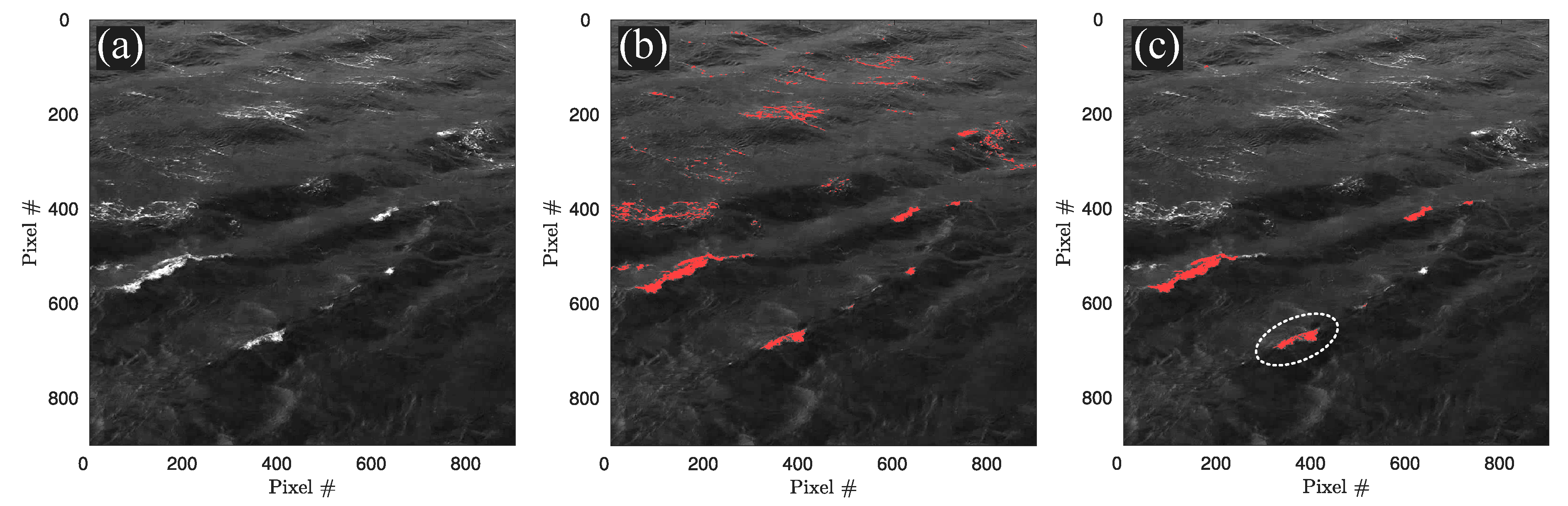
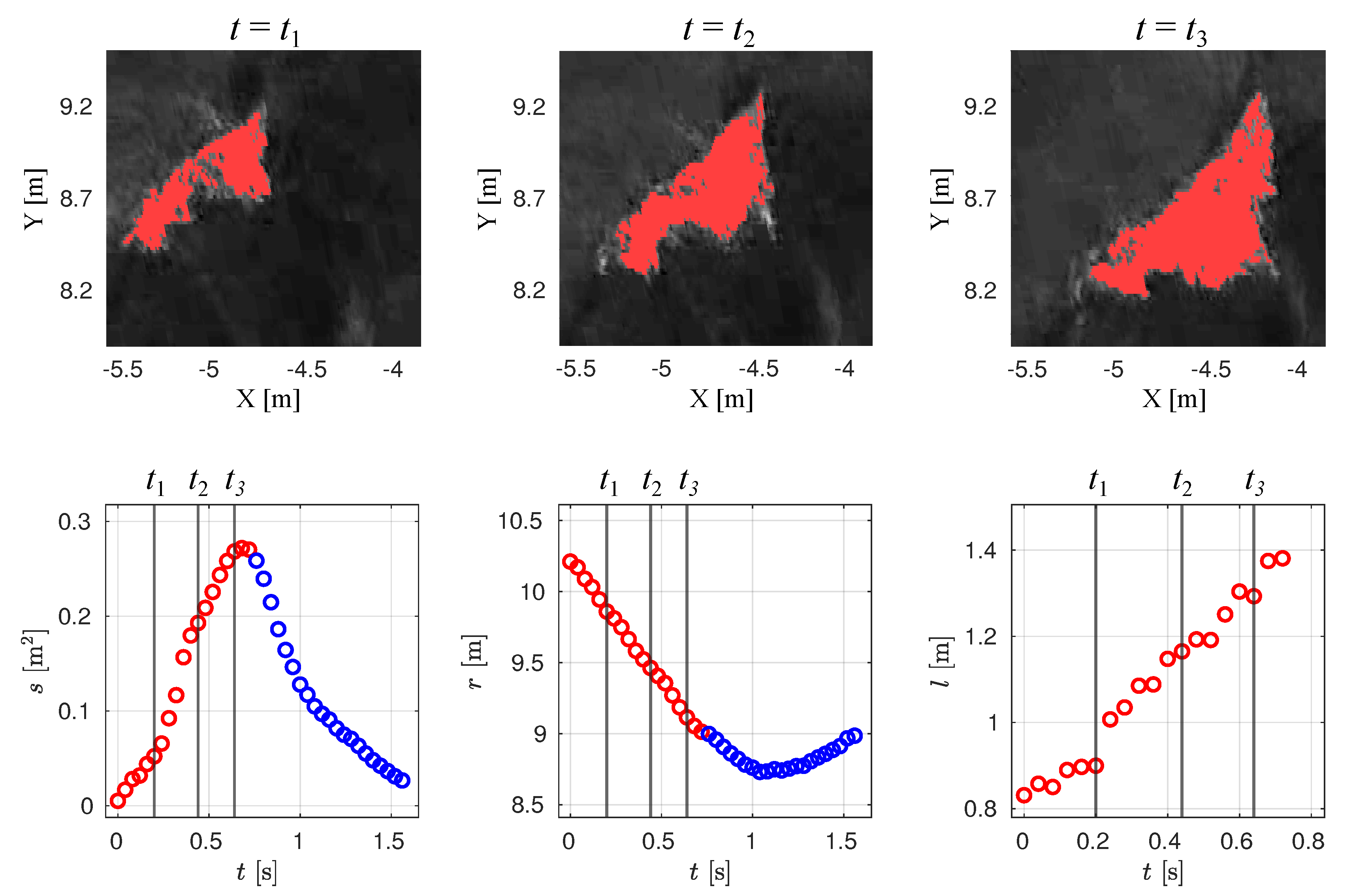
Some elements of the breaking wave detection procedure developed in [47] are shown in Figure 3 and Figure 4. Figure 3b illustrates a binarized image where foam from breaking waves (Figure 3a) is distinguished on the surface, using a threshold brightness. Figure 3c exhibits only active whitecaps (stage A foam) extracted from the binarized image, Figure 3b. In general, the extraction was performed through the analysis of time evolution of the area of an individual whitecap, Figure 4. Initially, the area grows and at some point starts to decrease, indicating that the breaking crest has disappeared and only residual foam is present for the rest of the time. The residual character of foam can also be seen in time evolution of the whitecap’s centroid position where the distance at the final stage of evolution exhibits oscillatory behaviour due to the wave orbital motion. For additional information on the algorithm see [47].
The final stage of video processing provided the following time-labeled attributes of individual breaking events: the average speed (or the phase speed) of a whitecap, cumulative sum of its areas, average whitecap length along the wave crest and the number of frames occupied by a breaking event. To make it clear what is measured and analysed in our work, hereafter we shall use the word instead of when referring to our experimental data.
Experimental estimates of and based on video recordings of the sea surface were derived as averages amongst successive frames
where and are the length and area of an individual whitecap in a given video frame, A is the observable surface area, is the number of frames, comprising a time interval and is the phase speed bin width. The summation in (3) is performed over individual breaking events and frames. To filter out rare fictitious breaking events, values of both and were assigned to zero in phase speed bins where the number of events was less than 5.
Examples of estimated , expressed in terms of f using (2) as , are shown in Figure 2 together with the number of events in each frequency bin. Other examples of and are shown in Figure 5 for each entry in Table 1 and Table 2. These figures will be discussed in the Results section.
The total length of whitecaps of dominant waves per unit surface area, (the total length of whitecaps for short), and the active whitecap coverage of these waves, , are defined as integrals of experimental estimates of and over the same spectral band as in (1):
2.3. Selection of Time Intervals
For the data analysis, we selected measurements confined to time intervals satisfying the following conditions: (i) an interval’s least squares wind acceleration did not exceed m s (it was also the requirement for the prior time interval to have a slowly changing wind speed), (ii) the wind direction standard deviation was below 10, and (iii) the number of breaking events of dominant waves was not less than 10 events.
In the onshore-wind conditions, statistical wave breaking parameters of dominant waves were calculated for consecutive 25 to 30 min-long time intervals. In the offshore-wind conditions, the fetches are short, i.e., it can take the field of breaking waves less than 25–30 min to reach the steady state. This point is important, since the number of days with offshore winds was small, and we needed to extract from such wind conditions as much information as possible.
Aiming to reduce the measurement interval and, therefore, increase the number of independent data samples, collected at different wind speeds, we needed to make sure that conditions of the wave field stationarity are satisfied for the selected time intervals. Following the theory of self-similarity of the wind-wave development [52] from the state of rest in fetch-limited conditions, the time, t, required for a front separating areas of fetch- and duration-limited wave growth to travel from a coast to a given point at a distance x, e.g., the research platform, is [53]:
where is dimensionless time, is a set of empirical constants for the fetch-limited wave growth and is dimensionless distance.
Fetches of typical offshore wind-waves, propagating from the Blue Gulf, vary from about 600 to 800 m. Adopting the empirical constants , [53] and substituting = 8–18 m s and x = 600–800 m to the above expression, we obtain the lower min and the upper min estimates of the time interval preceding the measurement, within which the stationarity of the wind is required to guarantee the stationary wave field.
3. Results
3.1. and Distributions
Examples of are shown in Figure 2. Swell waves were not observed to break in all the onshore- and offshore-wind cases, and the fastest whitecaps are attributed to dominant wind-waves. As anticipated, the number of detected breaking events is the smallest in the spectral peak region and rapidly increases towards higher wave frequencies. Subsequent roll-off in the number of events as a functions of f and values of at high frequencies (low phase speeds) is a known peculiarity of wave breaking data derived from visible video imagery.
This peculiarity originates from the fact that a regular video camera detects whitecaps that result from the air entrainment during the breaking process. At scales of short gravity waves with wavelengths less than 2 m, the surface tension starts to affect the breaking crest dynamics by reducing the intensity of the air entrainment and results in complete disappearance of whitecaps of decimeters-scale waves. Breaking continues to occur at small scales up to capillary wave scales, which is evident from infrared-camera recordings [54,55]. The measured by both infrared and visible video cameras are identical at phase speeds of breaking crests higher than 3 m s, but demonstrate significant difference at lower phase speeds: from visible imagery exhibits a considerable roll-off, whereas from infrared imagery increases towards the shortest gravity waves (see Figure 1 in [55] and Figure 6 in [35]).
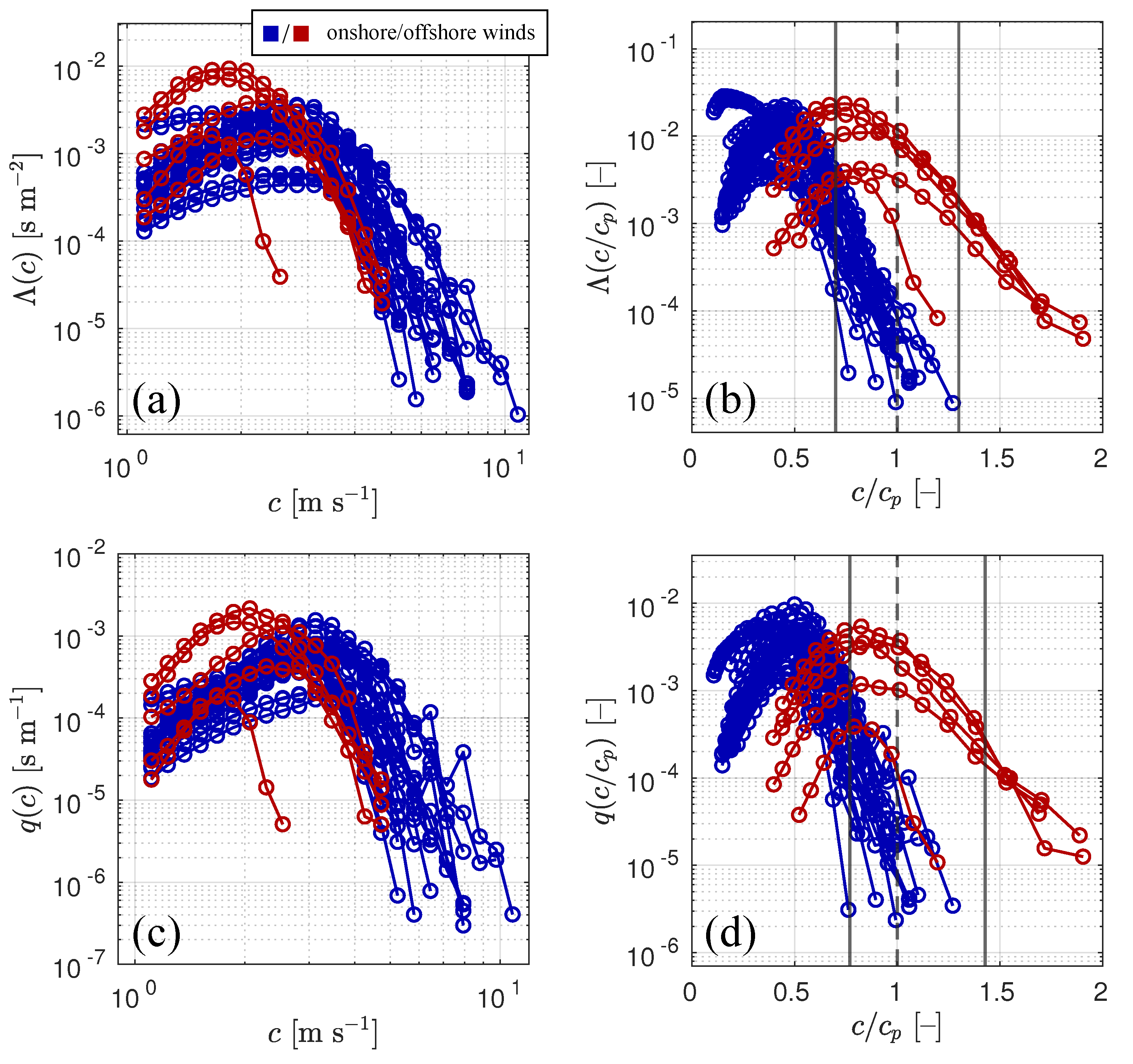
Our experimental estimates of and for both the onshore- and offshore-wind conditions (for each entry in Table 1 and Table 2) are shown in Figure 5a,c. Since the two wave breaking distributions have very similar spectral behaviour, below we focus on the analysis of only. In the range of the observed c, from 3 to 8 m s, values of decrease with the speed of whitecaps. Distributions at the offshore winds are more scattered than those in the onshore-wind conditions. Similar to , in at the onshore winds exhibits the roll-off behaviour at m s with the maximum around m s. As discussed above, such behaviour is presumably caused by the impact of the surface tension on the whitecap formation process associated with breaking of short gravity waves. It is seen in Figure 5c that the maxima of at the offshore winds are noticeably shifted towards low c relative to the corresponding maxima at the onshore winds. A possible reason for this is that the rate of a whitecaps production by steep offshore wind-waves is much greater than the production by onshore wind-wives in the same range of c (from 2 to 3 m s).
Functions and in Figure 5b,d clearly show that the peak of at the offshore winds relates to the spectral peak region where the surface tension apparently is not capable of suppressing generation of whitecaps of dominant waves. Unlike these cases, in the onshore-wind conditions takes minimal values around the spectral peak, suggesting that waves from the equilibrium range make the main contribution to Q.
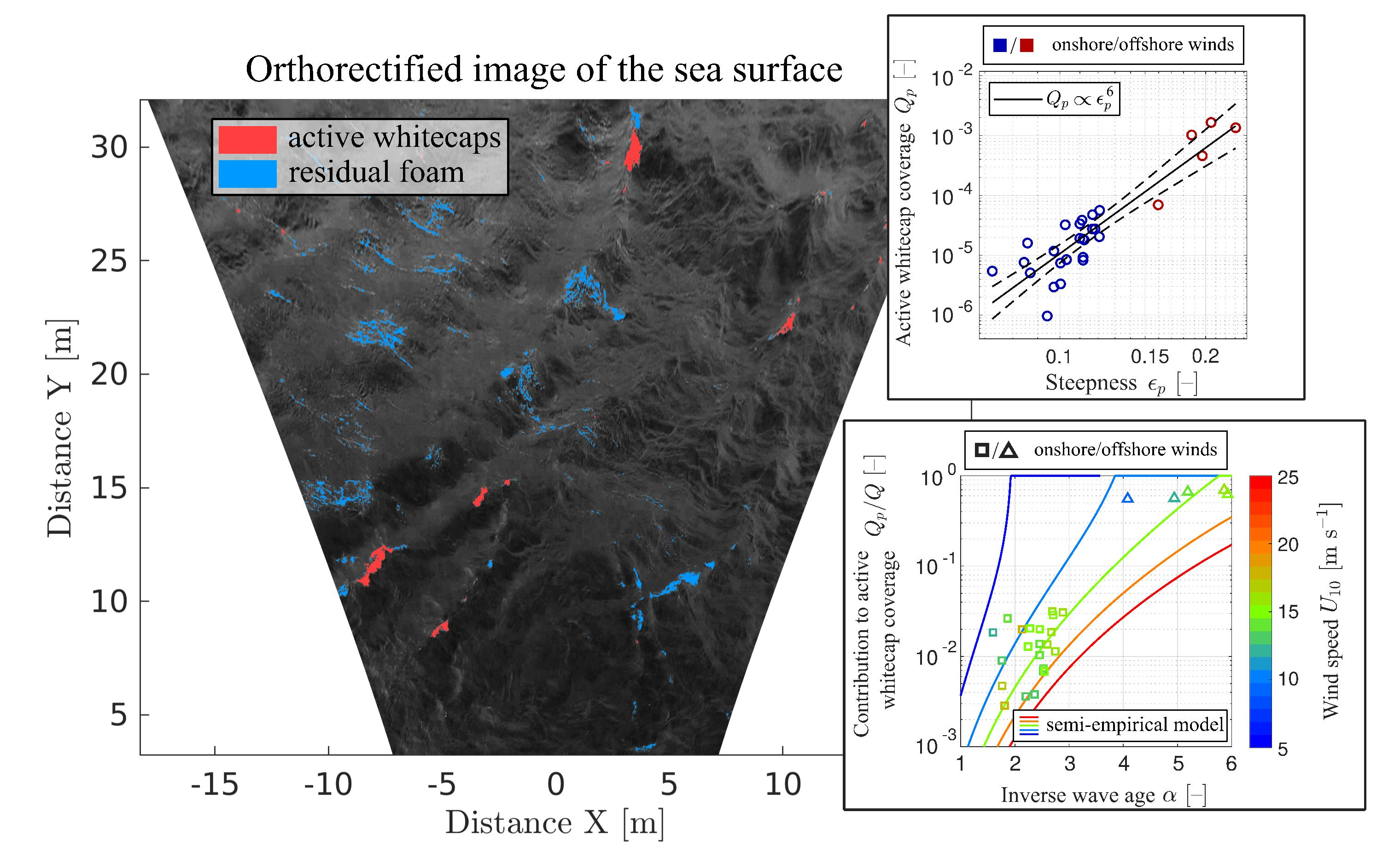
Figure 7a illustrates the contribution of dominant wave breaking to the total active whitecap coverage, Q. According to these estimates, young wind-waves associated with the offshore winds are responsible for 55.5% to 69.3%, for more than a half, of Q. More developed onshore wind-waves contribute 0.4–3.2% to Q. Figure 7b shows that the contribution of dominant waves to Q has no particular dependence on . Thus, from this results we conclude that the contribution of dominant waves to Q is not wind-speed, but wave-age dependent.
3.2. Dependencies of
Recently, authors [56] have proposed a parametric model of dominant waves developing under nonuniform wind fields. Within the model’s framework, the statistical parameters of the dominant wave breaking, and , exhibit a particular relationship to the dominant wave steepness, namely , which, following Toba’s fetch laws, transforms to , and . Below, we examine our experimental data for these relationships.
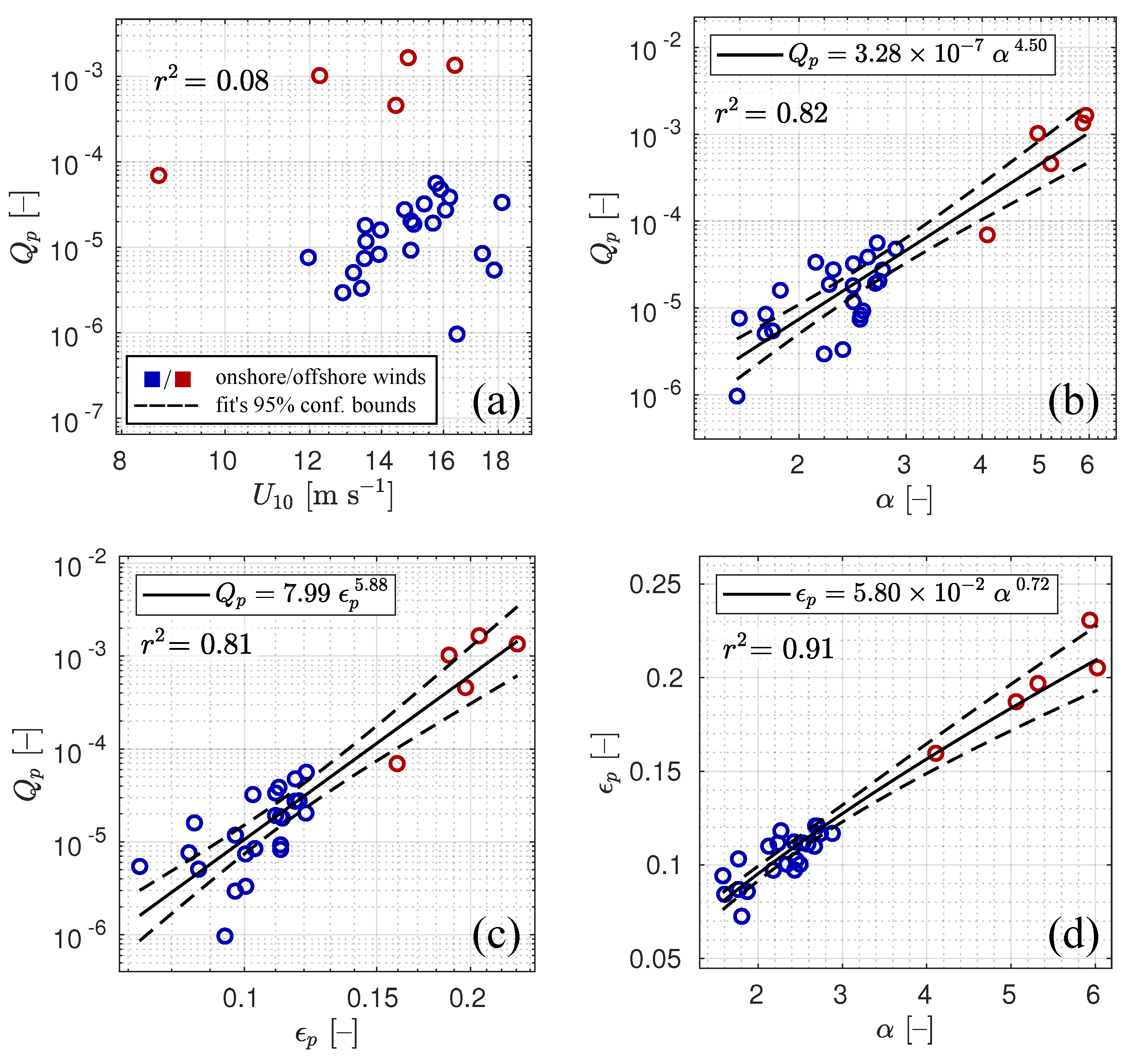
Firstly, the wind speed dependence of is illustrated in Figure 8a. The aggregated data (onshore and offshore-wind data) do not demonstrate any dependence of on . However, if we consider at the onshore and offshore winds separately, some wind-speed correlation can be revealed. This implies that there is another parameter, apart from the wind speed, that governs the breaking of dominant waves.
The active whitecap coverage of dominant waves represented as a function of the inverse wave age in Figure 8b demonstrates clear correlation. The produced by young wind-waves at the offshore winds attains values up to , whereas more developed onshore dominant waves have much lower values of , about . The power fit to the data points gives
The steepness of dominant waves is a fundamental parameter of the surface waves and serves as a measure of their nonlinearity [30]. Figure 8c demonstrates correlation of and with the power fit
High correlation of with both and is not surprising, since these quantities are related by the experimental fetch laws
shown in Figure 8d.
3.3. Dependencies of
Originally, was introduced for lengths of [33]. As far as visible video imagery is concerned, measured contains information about lengths of . Lengths of fast moving (and large scale) whitecaps of dominant waves in the onshore-wind conditions apparently correspond to lengths of breaking wave fronts. At the offshore winds dominant wind-waves are relatively short, and their breaking may be noticeably affected by the action of the surface tension. Possible evidence for that is the roll-off of at the offshore winds that takes place around phase speeds of dominant waves (see Figure 5b). In this case, the measured lengths of whitecaps are likely to be smaller than those of breaking wave fronts. To “recover” breaking front lengths of dominant waves, , in the offshore-wind conditions by “correcting” respective , we used a heuristic method described in Appendix B. Values of are provided in Table 2.
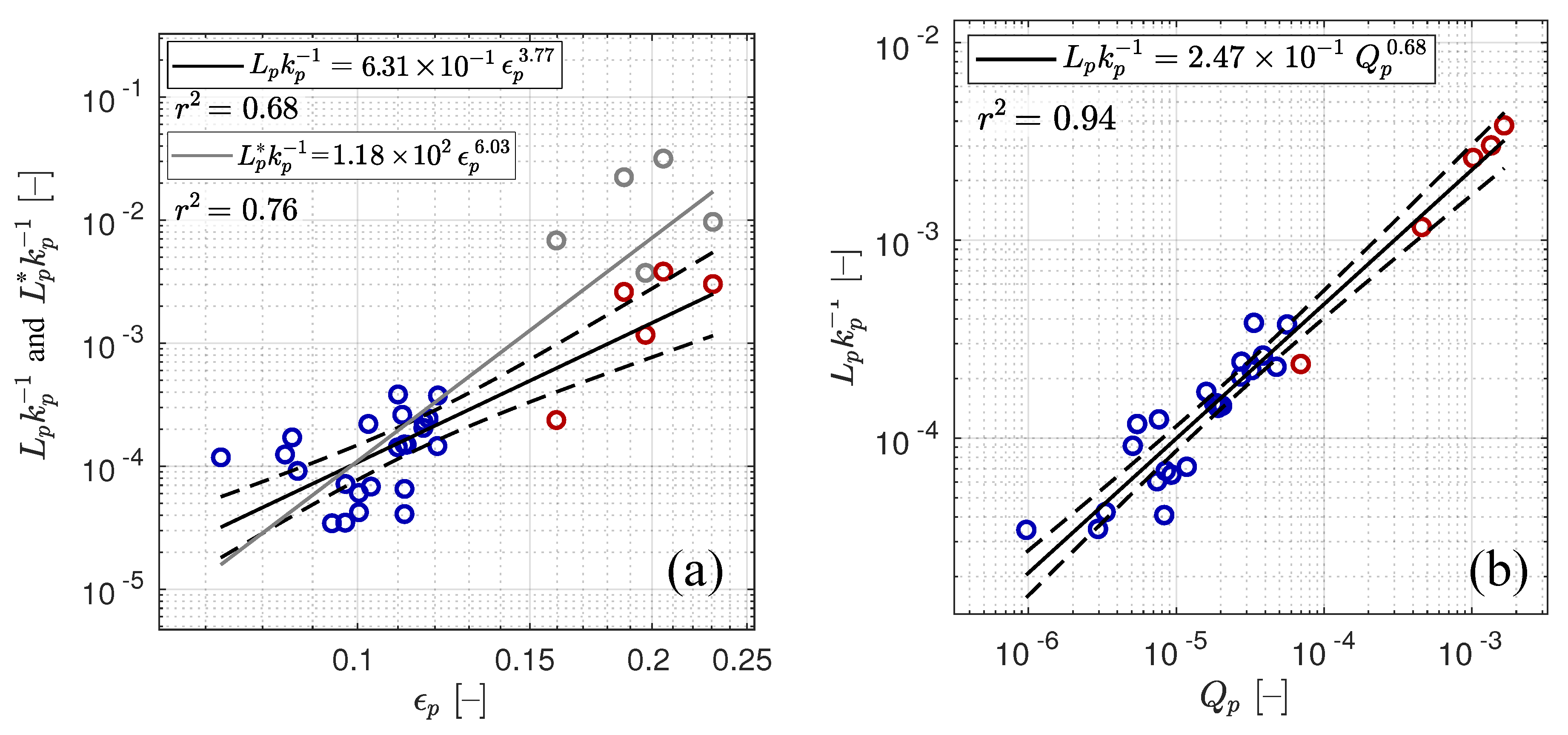
The experimental estimates of normalised by the spectral peak wavenumber as a function of is shown in Figure 9a. The power fit to the data points results in
where the exponent of the steepness is lower than the anticipated 6th power. If we use the recovered values that are only relevant to the offshore-wind cases, the power fit is enhanced giving a higher exponent for : .
Following ideas of Phillips [33] on self-similarity of geometric properties of breaking waves, the authors in [56] suggested that is proportional to . Our experimental data, shown in Figure 9b, demonstrate a deviation from the linear behaviour:
Such a deviation is probably caused by loss of self-similarity of whitecaps due to the action of the surface tension in the offshore-wind conditions as was mentioned in Section 3.1.
3.4. Dominant Wave Breaking Probability
Amongst statistical wave breaking parameters of dominant waves, a probability of breaking, , has drawn the most attention in the literature. Prior measurements of the wave breaking probability were reported in [29,30,31,32]. It was found that, besides the steepness of dominant waves, vertical surface current shear, finite depth and wave development stage can influence .
The dominant wave breaking probability—probability that a breaking crest of the dominant wave passes a fixed point on the sea surface—expressed in terms of reads [32]:
where is the passage rate of breaking crests of dominant waves past a fixed point, is the total passage rate of dominant wave crests that move with phase speeds in the range and 0.6 is an empirical constant (see [57] for details). Below we provide estimates of the probability derived from our measurements and compare them with the previously reported results.
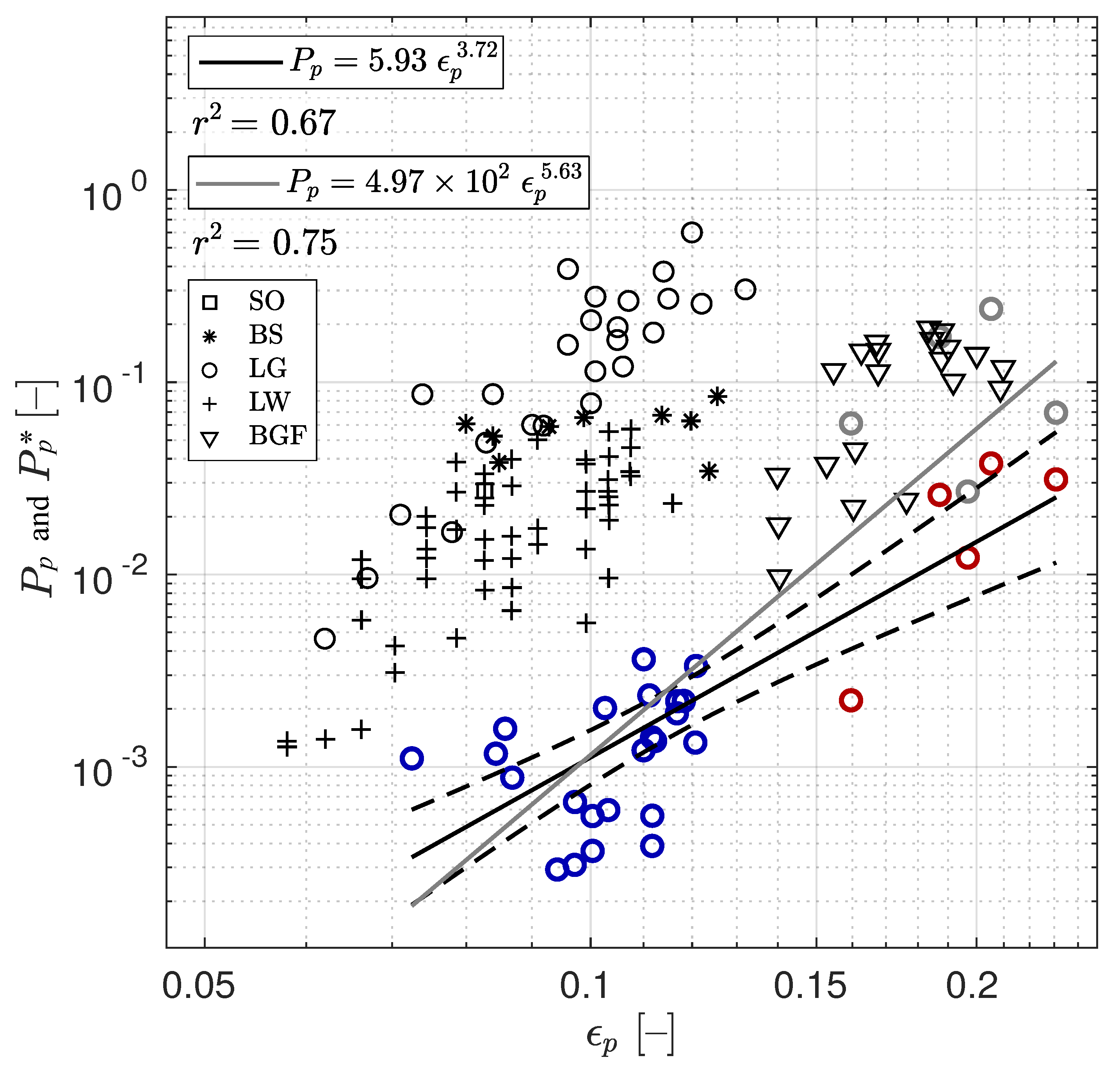
Figure 10 shows a dependence of , estimated from (10), on where we also show data from [29,30,31,32]. Values of are provided in Table 1 and Table 2. Comparing our data with previously reported observations, we arrive at interesting, if not confusing, conclusion: our estimates of at around 0.1 are by one—two orders of magnitude lower than the other Black Sea data reported earlier [30] and by two orders of magnitude lower than the Lake George data [31]. The probability of breaking of steep and young wind-waves at the offshore winds derived from lengths of whitecaps is at most 0.04, whereas the maximum probability in the same conditions derived from lengths of breaking fronts, , is 0.24. In our experiments, the number of breaking events of dominant waves with was negligible.
One possible reason for such a dramatic discrepancy may arise from the fact that the authors in [29,30,31] did not discriminate breaking crests of dominant waves from those of shorter waves occurring on crests of dominant waves. As found by [58], the effect of the modulation of short wave breaking by longer surface waves is very strong. They observed that breaking of short waves takes place on crests of longer waves and is practically absent in troughs. This phenomenon may lead to apparent overestimation of if short-scale and slow breaking events on crests of dominant waves are not filtered out when dealing with breaking of dominant waves. The speed of advance of whitecaps produced by dominant waves is significantly larger than the apparent speed of whitecaps of shorter waves (the sum of the intrinsic advance speed of whitecaps of short breaking waves and orbital velocity of dominant waves) riding the dominant wave crest. In our measurements, breaking events were differentiated according to speeds of whitecaps. Hence, we expect our estimates of to be lower than those reported by [29,30,31]. Data from [32] are closer to our measurements by an order of magnitude since the authors differentiated breaking of different spectral components.
The other possible reason lies in the dependence of the kinematic viscosity on sea water properties. Unlike the Black Sea case, less saline waters in lakes George and Washington have lower kinematic viscosity and therefore more dominant wave breaking is expected in these waters (see, e.g., [59]).
4. Discussion
4.1. Dissipation
As was mentioned in Section 1, the dissipation term in the wave energy balance equation is a function to be fitted to experimental data. For example, a source term in the WAM model describing the energy dissipation due to breaking has a form:
where d is a constant, e is the total wave energy, and denote weighted averages of the angular frequency and wavenumber, respectively, and is the surface elevation frequency spectrum (see Section 2.3.9 in [28]).
Integration of (11) over the spectral peak region to the first order gives
Alternatively, the rate of energy dissipation of dominant waves according to [33] is,
which, adopting the relationship as per [33], comes to
where in the last relationship we used found in the present study. The expression (13) coincides with (12), suggesting that our experimental data supports the dissipation term parameterization used in the WAM model.
4.2. Semi-Empirical Expression for Q
The most widely used parameterizations of the whitecap coverage are based on the wind speed scaling (see, e.g., Tables in [20,60]), but the scattering between these parameterizations is rather large. An alternative parametrization of the whitecap coverage involves the wave-age scaling [60,61]. However, use of the wave age as a parameter, when fitting to experimental data, does not result in a remarkable collapse of data points, as compared to the wind-speed scaling.
As a matter of fact, any integral parameter of wave breaking, e.g., the whitecap coverage, should depend on both the wind speed and wave age. On the one hand, breaking of equilibrium range waves provides dissipation of the energy, coming from the wind. Therefore, the contribution of these waves to integral wave breaking parameters is solely wind-speed dependent [33]. On the other hand, as found from our measurements, breaking parameters of spectral peak waves are dependent on the wave steepness and through the fetch laws—on the wave age.
Following this reasoning, it appears sensible to assume that the total active whitecap coverage can be represented as sum of the dominant wave, , and the equilibrium range wave, , contributions:
In line with [33], we describe wave breaking in the equilibrium range, assuming the balance between dissipation due to breaking and the wind energy input. As a consequence, is defined as:
where is the wave growth rate, is the saturation spectrum with n—the wave breaking dissipation exponent, parameterized as a power function of . Depending on a wave model, n varies from [33] to [62]. The quantity in (15) is a phase speed such that at the surface tension suppresses sharp crest disturbances triggering off the air entrainment, as mentioned in Section 3.1.
Combining the parameterization (6) (with the exponent of rounded to 6) with the expression (15) we arrive at the following semi-empirical expression of Q:
where is the Heaviside function with , chosen so vanishes when c of the entire spectral peak region are below set to 2 m s, constant corresponds to our experimental data (6), constant is chosen to match the data reported in [35] (see their Figure 4). The exponent n is set to 5 to be consistent with [62] and with the experimental findings of [35,63].
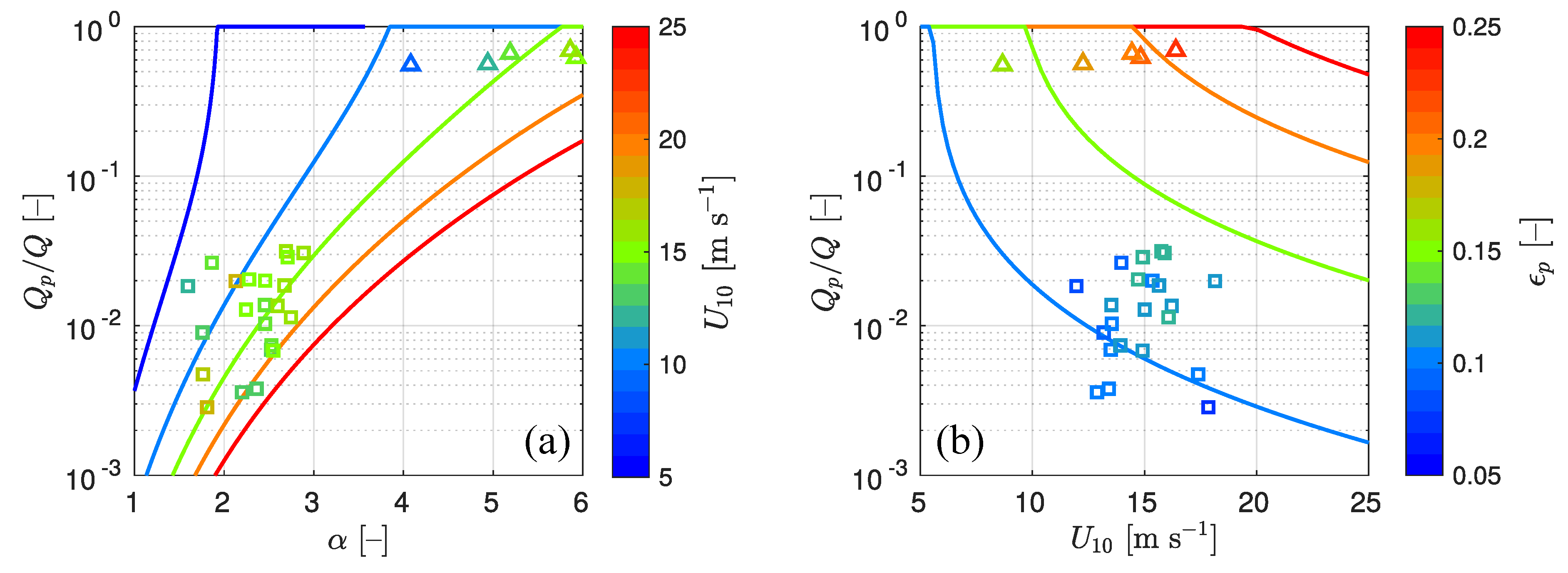
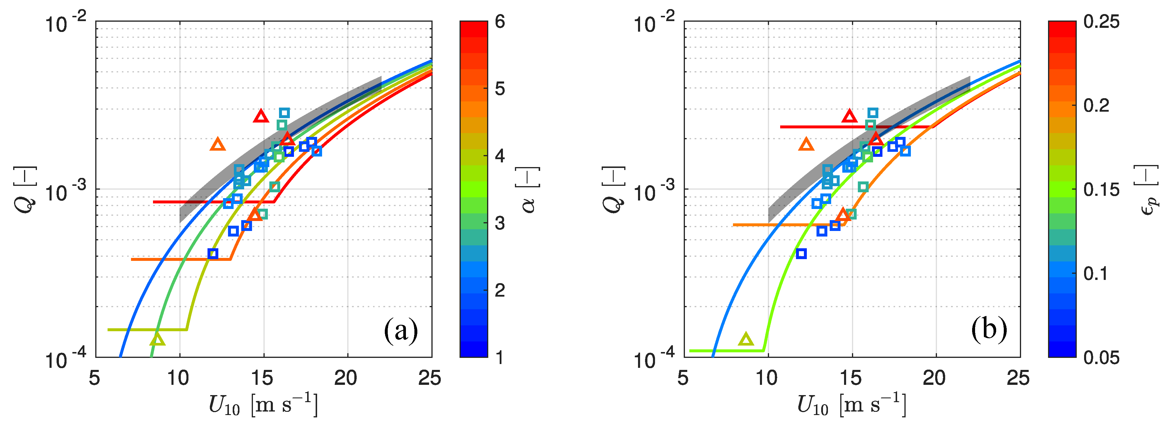
An example of model simulations of Q using (16) as a function of the wind speed for various and is shown in Figure 11. For mature seas at moderate and high winds, the spectral peak phase speed, , is significantly larger than . Since the contribution of dominant waves to Q in such conditions is small, Q is wholly governed by . In case of young seas, the spectral peak phase speed is close to , and, as a consequence, the contribution of the equilibrium range waves to Q becomes dependent on both the wind speed and inverse wave age. Thus, we see that at low , the scatter of the modelled Q is provided by the dominant waves and the dependence of on and ; Q is completely governed by at high wind speeds. It is interesting to note that the scatter of Q is much broader for the observed range of than for the range of .
When is used as a parameter for , our measurements show an unsatisfactory agreement with the modelled Q in Figure 11a. According to the semi-empirical model, at from 10 to 15 m s, Q is fully provided by , when is around 6, but our field data show that the equilibrium range has a nonzero contribution to the observed Q. Conversely, when is around 2, the experimental data is below the modelled Q. Our data for the intermediate have moderate agreement with the model. If we parameterize using directly, a better agreement between the model and data is seen at high (see Figure 11b).
Unlike the comparison with Q, in Figure 7 a better agreement is seen between the observed contribution of dominant waves to Q and the modelled one, although the model slightly overestimates the contribution of to Q in the offshore-wind conditions, predicting 100% contribution when the observed values do not exceed 80%.
5. Conclusions
This study presented the results of field investigations of dominant surface wave breaking in different wind and wave conditions. Very young waves were generated by offshore winds and mature surface waves travelled from the open sea. The wave breaking data were obtained at the Black Sea research platform using visible video imagery of the sea surface accompanied by co-located measurements of waves and wind. The active whitecap coverage and the total length of whitecaps of dominant waves were derived from spectral distributions of the active whitecap coverage, , and whitecap lengths .
As found, the contribution of dominant waves to the total active whitecap coverage, Q, depends on the inverse wave age, , and varies from 55.5% to 69.3%, when waves are young, and from 0.3% to 3.2%, when waves are mature.
The active whitecap coverage, produced by dominant waves, , exhibits a clear dependence on the dominant wave steepness, , showing proportionality to to the power of 6. This exponent supports the parametric model proposed in [56] as well as the dissipation term parameterization used in the WAM model. Since is related to the inverse wave age, also depends on .
We found that the dominant wave breaking probability, , is two orders of magnitude lower than the previously reported values [29,30,31]. Unlike the previous studies, in our measurements, all the detected whitecaps were differentiated according to the speed of their movement. Therefore, breaking of short, slow, and modulated waves on crests of dominant waves was filtered out.
In this study, we suggested a semi-empirical model for Q that takes into account separated contributions of breaking waves from spectral peak and equilibrium range intervals. According to this model, Q is a function of the wind speed and dominant wave steepness. The model predicts significant scatter of Q below m s at different inverse wave ages observed in our experiments.
The results of this study have possible and important applications to passive microwave remote sensing of the ocean surface. As dielectric properties of wave breaking foam are very different from those of water, microwave emmisivity of the ocean surface is significantly affected by breaking waves (see e.g., [20,64,65] and references cited therein). As argued by [23,24], C- and L-band microwave emission of the ocean surface may be dominated by large-scale breaking waves. At high wind conditions (e.g., in tropical and extra-tropical cyclones) dominant waves are strongly undeveloped. Whitecap coverage, produced by these waves, significantly contributes to the total Q. Since the large-scale breaking is capable of affecting L- and C-band emission of the ocean surface, reliable quantification of dominant wave breaking is vital to retrieve geophysical parameters from the satellite microwave data at the extreme conditions. Our results have possible applications for space-born altimeters as well: the so-called electromagnetic bias of the sea surface height is mainly caused by the different roughness of the sea surface on crests compared with that on troughs, which makes scattering nonuniform over the dominant wave profile and creates an offset between the mean scattering surface and the actual mean sea surface height [16,17].
Author Contributions
Conceptualization, V.N.K.; methodology, V.N.K., P.D.P., A.E.K. and V.V.M.; software, P.D.P. and A.E.K.; data acquisition, A.E.K. and V.V.M.; writing—original draft preparation, P.D.P.; writing—review and editing, P.D.P., V.N.K., A.E.K. and V.V.M.; visualization, P.D.P.; supervision, V.N.K. and V.V.M.; funding acquisition, V.N.K. and V.V.M. All authors have read and agreed to the published version of the manuscript.
Funding
The core support for this work was provided by the Russian Science Foundation through the Project No. 21-47-00038. The support of the Ministry of Science and Education of the Russian Federation under State Assignment No. 0555-2021-0004 at MHI RAS (data acquisition), and State Assignment No. 0763-2020-0005 at RSHU (data processing) are gratefully acknowledged.
Institutional Review Board Statement
Not applicable.
Informed Consent Statement
Not applicable.
Data Availability Statement
The data used in this study are provided in corresponding tables.
Acknowledgments
We would like to thank three anonymous referees whose valuable comments resulted in the improvement of the manuscript.
Conflicts of Interest
The authors declare no conflict of interest.
Appendix A. One-Dimensional Spectrum Partitioning
To perform partitioning of the frequency spectra, we assume that swell spectrum is narrow and can be approximated by a quadratic polynomial in the log-log domain.
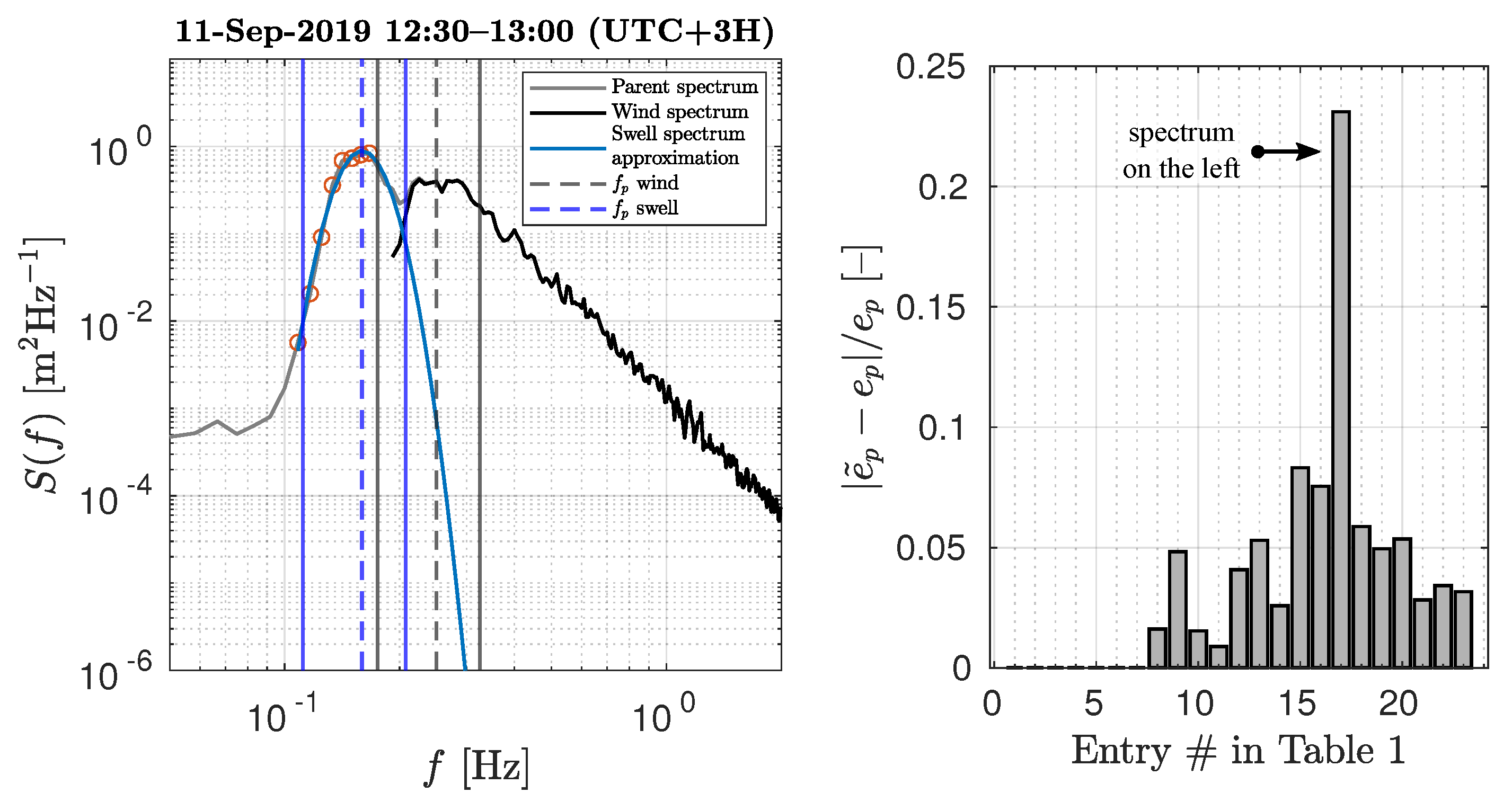
The procedure is the following. The spectral peak of wind-waves and the corresponding peak frequency are determined as described in the main text. At first, the swell spectral peak frequency, , is assigned manually. Then all the spectral points, that fall into the interval around the swell peak frequency, , provided they are out of the wind-wave spectral peak region, are used in the quadratic fit in the log-log domain. After the polynomial fit, is reassigned from the parabola, and the swell spectrum quadratic approximation is then subtracted from the original (parent) spectrum to give a refined wind-wave spectrum. This partition of wind-waves was further used to compute the energy and steepness of dominant waves. Application of this partitioning procedure and its impact on the energy of wind-waves is illustrated in Figure A1, where is the energy of dominant wind-waves, computed from the original spectrum, and is the same, but calculated from the partitioned one.
Figure A1.
() An example of swell and wind-wave systems separation in the frequency domain. The spectrum is from the upper left Figure 2. Orange circles show points used in the polynomial fit in the log-log domain. () Relative change in the energy of wind-waves after partitioning.
Figure A1.
() An example of swell and wind-wave systems separation in the frequency domain. The spectrum is from the upper left Figure 2. Orange circles show points used in the polynomial fit in the log-log domain. () Relative change in the energy of wind-waves after partitioning.

Appendix B. Offshore Λ(c)
In the offshore-wind conditions, the dominant wind-waves are relatively short and their breaking can be affected by the action of the surface tension. The latter suppresses sharp breaking crest disturbances that provide entrainment of the air, seen as whitecaps. Therefore, the lengths of the whitecaps may be smaller than those of the actually breaking fronts. In order to retrieve breaking front lengths, we suggest the following heuristic method.
The roll-off of in the range of c < 3 m s (see Figure 5a) can be regarded as an intrinsic feature of the lengths of the whitecaps, derived from visible video imagery [34,61,66,67]. However, infrared video recordings [54,55] suggest that the distribution of the lengths of the breaking fronts, , increases monotonically towards lower phase speeds up to micro-scale breaking associated with generation of parasitic capillaries.
We assume that the measured in the spectral peak region at the offshore winds may be corrupted by the effect of the surface tension (since the roll-off happens at the dominant wave scales) and, thus, is different from the “true” . In order to retrieve distributions of breaking front lengths from the measured , we introduce a correction function defined as,
To determine this function we use all available data at the onshore winds. Assuming that (see [33], which is supported by experimental data, e.g., [35,61]), we fit our data scaled by , , at m s by a power function of c with a prescribed exponent as in Figure A2. This fit is then extrapolated to the interval m s. The approximation by the power function was performed using the best linear fit in the log-log domain. The full power fit to our data at m s gives the exponent close to –6.
Deviation of the average at m s from the extrapolated is considered as an empirical estimate of the correction function ,
which is further used to retrieve breaking front lengths from the measured lengths of whitecaps.
Figure A2.
() Measured (gray lines) with their arithmetic average (black line). Vertical black line divides the range of phase speeds into the one used for the curve fitting (solid coloured lines) and for the extrapolation (dash coloured lines). () The correction function, , for both power approximations.

References
- Monahan, E.; Niocaill, G. Oceanic Whitecaps: And Their Role in Air-Sea Exchange Processes, 1st ed.; Oceanographic Sciences Library 2; Springer: Dordrecht, The Netherlands, 1986. [Google Scholar]
- Banner, M.; Peregrine, D. Wave Breaking in Deep Water. Annu. Rev. Fluid Mech. 1993, 25, 373–397. [Google Scholar] [CrossRef]
- Sharkov, E. Breaking Ocean Waves: Geometry, Structure and Remote Sensing; Springer Praxis Books; Springer: Berlin/Heidelberg, Germany, 2007. [Google Scholar]
- Babanin, A. Breaking and Dissipation of Ocean Surface Waves; Cambridge University Press: Cambridge, MA, USA, 2011. [Google Scholar]
- Bortkovskii, R. Air-Sea Exchange of Heat and Moisture during Storms; Springer: Berlin/Heidelberg, Germany, 1987; p. 194. [Google Scholar] [CrossRef]
- Thorpe, S. Dynamical processes of transfer at the sea surface. Prog. Oceanogr. 1995, 35, 315–352. [Google Scholar] [CrossRef]
- Melville, W. The Role of Surface-Wave Breaking in Air-Sea Interaction. Annu. Rev. Fluid Mech. 1996, 28, 279–321. [Google Scholar] [CrossRef]
- Makin, V.; Kudryavtsev, V. Impact Of Dominant Waves On Sea Drag. Bound.-Layer Meteorol. 2002, 103, 83–99. [Google Scholar] [CrossRef]
- Kudryavtsev, V.; Makin, V. Impact of Ocean Spray on the Dynamics of the Marine Atmospheric Boundary Layer. Bound.-Layer Meteorol. 2011, 140, 383–410. [Google Scholar] [CrossRef] [Green Version]
- Kudryavtsev, V.; Chapron, B.; Makin, V. Impact of wind waves on the air-sea fluxes: A coupled model. J. Geophys. Res. Ocean. 2014, 119, 1217–1236. [Google Scholar] [CrossRef] [Green Version]
- Kudryavtsev, V.; Hauser, D.; Caudal, G.; Chapron, B. A semiempirical model of the normalized radar cross-section of the sea surface 1. Background model. J. Geophys. Res. Ocean. 2003, 108. [Google Scholar] [CrossRef] [Green Version]
- Hwang, P.A.; Zhang, B.; Toporkov, J.V.; Perrie, W. Comparison of composite Bragg theory and quad-polarization radar backscatter from RADARSAT-2: With applications to wave breaking and high wind retrieval. J. Geophys. Res. Ocean. 2010, 115. [Google Scholar] [CrossRef] [Green Version]
- Kudryavtsev, V.N.; Fan, S.; Zhang, B.; Mouche, A.A.; Chapron, B. On Quad-Polarized SAR Measurements of the Ocean Surface. IEEE Trans. Geosci. Remote Sens. 2019, 57, 8362–8370. [Google Scholar] [CrossRef]
- Yurovsky, Y.Y.; Kudryavtsev, V.N.; Grodsky, S.A.; Chapron, B. Ka-Band Radar Cross-Section of Breaking Wind Waves. Remote Sens. 2021, 13, 1929. [Google Scholar] [CrossRef]
- Yurovsky, Y.Y.; Kudryavtsev, V.N.; Grodsky, S.A.; Chapron, B. Sea Surface Ka-Band Doppler Measurements: Analysis and Model Development. Remote Sens. 2019, 11, 839. [Google Scholar] [CrossRef]
- Reale, F.; Dentale, F.; Carratelli, E.P. Numerical Simulation of Whitecaps and Foam Effects on Satellite Altimeter Response. Remote Sens. 2014, 6, 3681–3692. [Google Scholar] [CrossRef] [Green Version]
- Gommenginger, C.; Srokosz, M. Sea state bias—20 years on. In Proceedings of the Symposium on 15 Years of Progress in Radar Altimetry, Venice, Italy, 13–18 March 2006 (ESA SP-614, July 2006); Danesy, D., Ed.; ESA Publications Division: Noordwijk, The Netherlands, 2006. [Google Scholar]
- Reale, F.; Dentale, F.; Carratelli, E.P.; Fenoglio-Marc, L. Influence of Sea State on Sea Surface Height Oscillation from Doppler Altimeter Measurements in the North Sea. Remote Sens. 2018, 10, 1100. [Google Scholar] [CrossRef] [Green Version]
- Quartly, G.D.; Chen, G.; Nencioli, F.; Morrow, R.; Picot, N. An Overview of Requirements, Procedures and Current Advances in the Calibration/Validation of Radar Altimeters. Remote Sens. 2021, 13, 125. [Google Scholar] [CrossRef]
- Anguelova, M.; Webster, F. Whitecap coverage from satellite measurements: A first step toward modeling the variability of oceanic whitecaps. J. Geophys. Res. Ocean. 2006, 111. [Google Scholar] [CrossRef] [Green Version]
- Hwang, P. Foam and Roughness Effects on Passive Microwave Remote Sensing of the Ocean. IEEE Trans. Geosci. Remote Sens. 2012, 50, 2978–2985. [Google Scholar] [CrossRef]
- Anguelova, M.D. Global Whitecap Coverage from Satellite Remote Sensing and Wave Modelling. In Recent Advances in the Study of Oceanic Whitecaps. Twixt Wind and Waves; Vlahos, P., Monahan, E., Eds.; Springer: Berlin/Heidelberg, Germany, 2020; Chapter 11; pp. 153–174. [Google Scholar]
- Reul, N.; Chapron, B. A model of sea-foam thickness distribution for passive microwave remote sensing applications. J. Geophys. Res. Ocean. 2003, 108. [Google Scholar] [CrossRef] [Green Version]
- Reul, N.; Tenerelli, J.; Chapron, B.; Vandemark, D.; Quilfen, Y.; Kerr, Y. SMOS satellite L-band radiometer: A new capability for ocean surface remote sensing in hurricanes. J. Geophys. Res. Ocean. 2012, 117. [Google Scholar] [CrossRef] [Green Version]
- Bowyer, P.J.; MacAfee, A.W. The Theory of Trapped-Fetch Waves with Tropical Cyclones—An Operational Perspective. Weather Forecast. 2005, 20, 229–244. [Google Scholar] [CrossRef]
- Kudryavtsev, V.; Golubkin, P.; Chapron, B. A simplified wave enhancement criterion for moving extreme events. J. Geophys. Res. Ocean. 2015, 120, 7538–7558. [Google Scholar] [CrossRef] [Green Version]
- Komen, G.J.; Cavaleri, L.; Donelan, M.; Hasselmann, K.; Hasselmann, S.; Janssen, P.A.E.M. Dynamics and Modelling of Ocean Waves; Cambridge University Press: Cambridge, MA, USA, 1994. [Google Scholar] [CrossRef]
- NOAA/NWS/NCEP/MMAB. User Manual and System Documentation of WAVEWATCHIII Version 6.07; Tech. Note 333; NOAA/NWS/NCEP/MMAB: College Park, MD, USA, 2019.
- Katsaros, K.; Atakturk, S. Dependence of wave-breaking statistics on wind stress and wave developmen. In Breaking Waves; Banner, M., Grimshaw, R., Eds.; Springer: Berlin/Heidelberg, Germany, 1992; pp. 119–132. [Google Scholar]
- Banner, M.; Babanin, A.; Young, I. Breaking Probability for Dominant Waves on the Sea Surface. J. Phys. Oceanogr. 2000, 30, 3145–3160. [Google Scholar] [CrossRef]
- Babanin, A.; Young, I.; Banner, M. Breaking probabilities for dominant surface waves on water of finite constant depth. J. Geophys. Res. Ocean. 2001, 106, 11659–11676. [Google Scholar] [CrossRef]
- Banner, M.; Gemmrich, J.; Farmer, D. Multiscale Measurements of Ocean Wave Breaking Probability. J. Phys. Oceanogr. 2002, 32, 3364–3375. [Google Scholar] [CrossRef]
- Phillips, O. Spectral and statistical properties of the equilibrium range in wind-generated gravity waves. J. Fluid Mech. 1985, 156, 505–531. [Google Scholar] [CrossRef]
- Korinenko, A.; Malinovsky, V.; Kudryavtsev, V. Experimental Research of Statistical Characteristics of Wind Wave Breaking. Phys. Oceanogr. 2018, 25, 489–500. [Google Scholar] [CrossRef] [Green Version]
- Korinenko, A.; Malinovsky, V.; Kudryavtsev, V.; Dulov, V. Statistical Characteristics of Wave Breakings and their Relation with the Wind Waves’ Energy Dissipation Based on the Field Measurements. Phys. Oceanogr. 2020, 27. [Google Scholar] [CrossRef]
- Fairall, C.; Bradley, E.; Hare, J.; Grachev, A.; Edson, J. Bulk Parameterization of Air–Sea Fluxes: Updates and Verification for the COARE Algorithm. J. Clim. 2003, 16, 571–591. [Google Scholar] [CrossRef]
- Earle, M.; Brown, R.; Baker, D.; McCall, J. Nondirectional and Directional Wave Data Analysis Procedures; U.S. Department of Commerce, National Oceanic and Atmospheric Administration, National Data Buoy Center: Slidell, LA, USA, 1996. Available online: www.ndbc.noaa.gov/wavemeas.pdf (accessed on 2 April 2021).
- Hashimoto, N.; Nagai, T.; Asai, T. Extension of the Maximum Entropy Principle Method for Directional Wave Spectrum Estimation. In Coastal Engineering 1994; 1994; pp. 232–246. [Google Scholar] [CrossRef]
- Johnson, D. DIWASP, a Directional Wave Spectra Toolbox for MATLAB: User Manual; Res. Rep. WP-1601-DJ (V1.1); Centre Water Reseach, University Western Australia: Crawley, WA, Australia, 2002. [Google Scholar]
- Hanson, J.; Phillips, O. Wind Sea Growth and Dissipation in the Open Ocean. J. Phys. Oceanogr. 1999, 29, 1633–1648. [Google Scholar] [CrossRef]
- Toba, Y. Local balance in the air-sea boundary processes. J. Oceanogr. Soc. Jpn. 1973, 29, 209–220. [Google Scholar] [CrossRef]
- Pierson, W.; Moskowitz, L. A Proposed Spectral Form for Fully Developed Wind Seas Based on the Similarity Theory of S. A. Kitaigorodskii. J. Geophys. Res. 1964, 69, 5181–5190. [Google Scholar] [CrossRef]
- Hasselmann, K.; Barnett, T.; Bouws, E.; Carlson, H.; Cartwright, D.; Enke, K.; Ewing, J.; Gienapp, H.; Hasselmann, D.; Kruseman, P.; et al. Measurements of wind-wave growth and swell decay during the Joint North Sea Wave Project (JONSWAP). Deutches Hydrogr. Inst. 1973, 8, 1–95. [Google Scholar]
- Rapp, R.; Melville, W. Laboratory measurements of deep-water breaking waves. Philos. Trans. R. Soc. Lond. Ser. A Math. Phys. Sci. 1990, 331, 735–800. [Google Scholar] [CrossRef] [Green Version]
- Stansell, P.; MacFarlane, C. Experimental Investigation of Wave Breaking Criteria Based on Wave Phase Speeds. J. Phys. Oceanogr. 2002, 32, 1269–1283. [Google Scholar] [CrossRef]
- Banner, M.; Peirson, W. Wave breaking onset and strength for two-dimensional deep-water wave groups. J. Fluid Mech. 2007, 585, 93–115. [Google Scholar] [CrossRef] [Green Version]
- Mironov, A.; Dulov, V. Detection of wave breaking using sea surface video records. Meas. Sci. Technol. 2007, 19, 015405. [Google Scholar] [CrossRef]
- Anguelova, M.; Hwang, P. Using Energy Dissipation Rate to Obtain Active Whitecap Fraction. J. Phys. Oceanogr. 2016, 46, 461–481. [Google Scholar] [CrossRef]
- Monahan, E.; Woolf, D. Comments on “Variations of Whitecap Coverage with Wind stress and Water Temperature”. J. Phys. Oceanogr. 1989, 19, 706–709. [Google Scholar] [CrossRef] [Green Version]
- Bondur, V.; Sharkov, E. Statistical properties of whitecaps on a rough sea. Oceanology 1982, 22, 274–279. [Google Scholar]
- Bouguet, J.Y. Camera Calibration Toolbox for Matlab; Computational Vision at the California Institute of Technology: Pasadena, CA, USA; Available online: http://www.vision.caltech.edu/bouguetj/calib_doc/ (accessed on 12 July 2021).
- Kitaigorodskii, S. The Physics of Air-Sea Interaction; Israel Program for Scientific Translation Publisher: Jerusalem, Israel, 1973. [Google Scholar]
- Dulov, V.; Kudryavtsev, V.; Skiba, E. On fetch- and duration-limited wind wave growth: Data and parametric model. Ocean Model. 2020, 153, 101676. [Google Scholar] [CrossRef]
- Jessup, A.; Phadnis, K. Measurement of the geometric and kinematic properties of microscale breaking waves from infrared imagery using a PIV algorithm. Meas. Sci. Technol. 2005, 16, 1961–1969. [Google Scholar] [CrossRef]
- Sutherland, P.; Melville, W. Field measurements and scaling of ocean surface wave-breaking statistics. Geophys. Res. Lett. 2013, 40, 3074–3079. [Google Scholar] [CrossRef]
- Kudryavtsev, V.; Yurovskaya, M.; Chapron, B. 2D parametric model for surface wave development under varying wind field in space and time. J. Geophys. Res. Ocean. 2021, 126. [Google Scholar] [CrossRef]
- Banner, M.; Morison, R. Refined source terms in wind wave models with explicit wave breaking prediction. Part I: Model framework and validation against field data. Ocean Model. 2010, 33, 177–189. [Google Scholar] [CrossRef]
- Dulov, V.; Kudryavtsev, V.; Bol’Shakov, A. A Field Study of Whitecap Coverage and its Modulations by Energy Containing Surface Waves. In Gas Transfer at Water Surfaces; American Geophysical Union (AGU): Washington, DC, USA, 2002; pp. 187–192. [Google Scholar] [CrossRef]
- Anguelova, M.D.; Huq, P. Effects of Salinity on Surface Lifetime of Large Individual Bubbles. J. Mar. Sci. Eng. 2017, 5, 41. [Google Scholar] [CrossRef]
- Brumer, S.; Zappa, C.; Brooks, I.; Tamura, H.; Brown, S.; Blomquist, B.; Fairall, C.; Cifuentes-Lorenzen, A. Whitecap Coverage Dependence on Wind and Wave Statistics as Observed during SO GasEx and HiWinGS. J. Phys. Oceanogr. 2017, 47, 2211–2235. [Google Scholar] [CrossRef]
- Kleiss, J.; Melville, W. Observations of Wave Breaking Kinematics in Fetch-Limited Seas. J. Phys. Oceanogr. 2010, 40, 2575–2604. [Google Scholar] [CrossRef]
- Donelan, M.A.; Pierson, W.J. Radar scattering and equilibrium ranges in wind-generated waves with application to scatterometry. J. Geophys. Res. Ocean. 1987, 92, 4971–5029. [Google Scholar] [CrossRef]
- Dulov, V.A.; Korinenko, A.E.; Kudryavtsev, V.N.; Malinovsky, V.V. Modulation of Wind-Wave Breaking by Long Surface Waves. Remote Sens. 2021, 13, 2825. [Google Scholar] [CrossRef]
- Anguelova, M. Complex dielectric constant of sea foam at microwave frequencies. J. Geophys. Res. Ocean. 2008, 113. [Google Scholar] [CrossRef] [Green Version]
- Hwang, P.; Reul, N.; Meissner, T.; Yueh, S. Whitecap and Wind Stress Observations by Microwave Radiometers: Global Coverage and Extreme Conditions. J. Phys. Oceanogr. 2019, 49, 2291–2307. [Google Scholar] [CrossRef]
- Melville, W.; Matusov, P. Distribution of breaking waves at the ocean surface. Nature 2002, 417, 58–63. [Google Scholar] [CrossRef] [PubMed]
- Gemmrich, J.; Banner, M.; Garrett, C. Spectrally Resolved Energy Dissipation Rate and Momentum Flux of Breaking Waves. J. Phys. Oceanogr. 2008, 38, 1296–1312. [Google Scholar] [CrossRef]
Figure 1.
Location of the Black Sea research platform and a general view on the instrumentation.

Figure 2.
(left column) Frequency spectra, , spectral distribution of the total length of whitecaps, , and detected number of breaking events. Dashed vertical lines indicate spectral peak frequencies, ( corresponds to the Pierson-Moskowitz frequency) and solid vertical lines indicate spectral peak intervals built from swell and wind-waves . Shaded blue area around shows 95% confidence intervals. (right column) Directional wave spectra, , where arrows show the wind direction. Figures in the top row are for a time interval of onshore winds on 11 September 2019, and those in the bottom row are for a time interval of offshore winds on 25 September 2013.

Figure 3.
() An example of a grayscale image of the sea surface with breaking waves on 24 September 2013 at around 12:34 (UTC + 3H). () The same with detected foam using brightness threshold and () with extracted active foam. A breaking crest outlined in plot (c) is shown in Figure 4.
Figure 3.
() An example of a grayscale image of the sea surface with breaking waves on 24 September 2013 at around 12:34 (UTC + 3H). () The same with detected foam using brightness threshold and () with extracted active foam. A breaking crest outlined in plot (c) is shown in Figure 4.

Figure 4.
() A sequence of orthorectified frames with the whitecap outlined in Figure 3c. () The area, distance of the whitecap’s centroid from an arbitrary origin, and length of the whitecap as a function of time. Red and blue markers indicate stage A and stage B breaking, respectively. Vertical black lines show time moments corresponding to the above frames.

Figure 5.
(a,b) The distributions as a function of c and , where is the peak phase speed. (c,d) The same, but for q distributions.
Figure 5.
(a,b) The distributions as a function of c and , where is the peak phase speed. (c,d) The same, but for q distributions.

Figure 6.
() Wind speed, and direction, time series for a video record in the onshore-wind conditions. () The same, but in the offshore-wind conditions. Black lines are 15-min-average wind speed. Black vertical thick lines indicate time intervals of continuous video recordings of the sea surface. Shaded gray rectangles indicate time intervals, for which the wave spectra and statistical wave breaking parameters of dominant waves were estimated and shown in Figure 2.

Figure 7.
() The contribution of dominant waves to the observed total active whitecap coverage, Q, as a function of the inverse wave age, . () The same, but as a function of the wind speed, . Squares and triangles correspond to the onshore- and offshore-wind conditions, respectively. Lines indicate calculations from a semi-empirical model of Q, introduced in Section 4, for different and dominant wave steepness, .

Figure 8.
() The active whitecap coverage of dominant waves, , as a function of the wind speed, , () inverse wave age, , and () dominant wave steepness, , () The as a function of . In the subfigures, a squared correlation coefficient, , and confidence bounds are based on the best linear fit in the log–log domain. For the colour-coding see the legend.

Figure 9.
(). The total length of whitecaps of dominant waves per unit surface area, , normalised by the peak wavenumber, , as a function of the dominant wave steepness, . () The same quantity, but as a function of the active whitecap coverage of dominant waves, . Notation and colour-coding are the same as in Figure 8. Gray markers are for the recovered at the offshore winds, which represents the total length of the breaking fronts of dominant waves. The gray line corresponds to the power fit to the total cloud of points when red markers are replaced with gray ones.

Figure 10.
Estimated probability of dominant wave breaking, , as a function of the dominant wave steepness, , together with previously reported field data, shown as black markers. In the legend: SO—Southern Ocean, BS—Black Sea, LG—Lake George, LW—Lake Washington data described in [30,31], and BGF—data points of [32]. Notation and colour-coding are the same as in Figure 8 and Figure 9. Gray markers are for the at the offshore winds. The gray line corresponds to the power fit to the total cloud of points when red markers are replaced with gray ones.

Figure 11.
(). The semi-empirical total active whitecap coverage, Q, as a function of the wind speed, , for different inverse wave ages, . () The same, but for different dominant wave steepness, . Markers represent our experimental estimates of Q. Squares and triangles correspond to the onshore- and offshore-wind conditions, respectively. A thick gray line indicates the parameterization of [35].


Table 1.
Wind data, wave and wave breaking parameters of dominant wind-waves in the onshore-wind conditions. In the table, and is the wind speed and direction at 10 m height, is the wave propagation direction, is the inverse wave age, are the frequency, energy and steepness of dominant waves, and are the total length of whitecaps per unit surface area and the active whitecap coverage of dominant waves, respectively, is the dominant wave breaking probability and N is the number of breaking events of dominant waves.
| # | Date (Time in UTC + 3H) | N | ||||||||||
|---|---|---|---|---|---|---|---|---|---|---|---|---|
| 1 * | 13 October 2018 10:12–10:42 | 17.8 | 77.4 | – | 1.8 | 1.6 × 10⁻¹ | 1.3 × 10⁻¹ | 7.3 × 10⁻² | 1.2 × 10⁻⁵ | 5.4 × 10⁻⁶ | 1.1 × 10⁻³ | 223 |
| 2 * | 13 October 2018 10:42–11:08 | 18.1 | 75.5 | – | 2.1 | 1.8 × 10⁻¹ | 1.7 × 10⁻¹ | 1.1 × 10⁻¹ | 5.2 × 10⁻⁵ | 3.4 × 10⁻⁵ | 3.6 × 10⁻³ | 750 |
| 3 * | 14 October 2018 09:05–09:35 | 16.5 | 69.2 | – | 1.6 | 1.5 × 10⁻¹ | 2.7 × 10⁻¹ | 9.4 × 10⁻² | 3.1 × 10⁻⁶ | 9.7 × 10⁻⁷ | 3.0 × 10⁻⁴ | 14 |
| 4 * | 14 October 2018 09:35–10:05 | 17.4 | 65.8 | – | 1.8 | 1.6 × 10⁻¹ | 2.6 × 10⁻¹ | 1.0 × 10⁻¹ | 6.9 × 10⁻⁶ | 8.5 × 10⁻⁶ | 6.0 × 10⁻⁴ | 13 |
| 5 * | 15 October 2018 09:58–10:28 | 12.0 | 77.0 | – | 1.6 | 2.1 × 10⁻¹ | 5.8 × 10⁻² | 8.4 × 10⁻² | 2.2 × 10⁻⁵ | 7.6 × 10⁻⁶ | 1.2 × 10⁻³ | 413 |
| 6 * | 15 October 2018 10:28–10:58 | 13.2 | 75.4 | – | 1.8 | 2.1 × 10⁻¹ | 6.2 × 10⁻² | 8.7 × 10⁻² | 1.6 × 10⁻⁵ | 5.1 × 10⁻⁶ | 9.0 × 10⁻⁴ | 296 |
| 7 * | 15 October 2018 11:06–11:36 | 14.0 | 76.7 | – | 1.9 | 2.1 × 10⁻¹ | 6.0 × 10⁻² | 8.6 × 10⁻² | 3.0 × 10⁻⁵ | 1.6 × 10⁻⁵ | 1.6 × 10⁻³ | 469 |
| 8 | 10 September 2019 10:01–10:31 | 13.4 | 90.0 | 81.3 | 2.4 | 2.8 × 10⁻¹ | 3.0 × 10⁻² | 1.1 × 10⁻¹ | 4.8 × 10⁻⁵ | 1.8 × 10⁻⁵ | 1.4 × 10⁻³ | 313 |
| 9 | 10 September 2019 10:31–11:01 | 13.4 | 90.0 | 81.9 | 2.4 | 2.8 × 10⁻¹ | 2.3 × 10⁻² | 9.7 × 10⁻² | 2.3 × 10⁻⁵ | 1.2 × 10⁻⁵ | 7.0 × 10⁻⁴ | 92 |
| 10 | 10 September 2019 11:01–11:31 | 13.4 | 90.0 | 91.7 | 2.5 | 2.9 × 10⁻¹ | 2.1 × 10⁻² | 1.0 × 10⁻¹ | 2.1 × 10⁻⁵ | 7.4 × 10⁻⁶ | 6.0 × 10⁻⁴ | 119 |
| 11 | 10 September 2019 11:31–11:57 | 13.3 | 90.0 | 93.3 | 2.3 | 2.8 × 10⁻¹ | 2.7 × 10⁻² | 1.0 × 10⁻¹ | 1.3 × 10⁻⁵ | 3.3 × 10⁻⁶ | 4.0 × 10⁻⁴ | 112 |
| 12 | 10 September 2019 12:01–12:31 | 12.8 | 90.0 | 95.1 | 2.2 | 2.7 × 10⁻¹ | 2.9 × 10⁻² | 9.7 × 10⁻² | 9.9 × 10⁻⁶ | 3.0 × 10⁻⁶ | 3.0 × 10⁻⁴ | 82 |
| 13 | 10 September 2019 12:31–13:01 | 13.8 | 90.0 | 93.7 | 2.5 | 2.8 × 10⁻¹ | 3.0 × 10⁻² | 1.1 × 10⁻¹ | 1.3 × 10⁻⁵ | 8.3 × 10⁻⁶ | 4.0 × 10⁻⁴ | 70 |
| 14 | 10 September 2019 13:01–13:31 | 14.8 | 90.0 | 91.7 | 2.5 | 2.7 × 10⁻¹ | 3.8 × 10⁻² | 1.1 × 10⁻¹ | 1.9 × 10⁻⁵ | 9.3 × 10⁻⁶ | 6.0 × 10⁻⁴ | 74 |
| 15 | 11 September 2019 11:30–12:00 | 14.7 | 90.0 | 87.8 | 2.3 | 2.4 × 10⁻¹ | 6.3 × 10⁻² | 1.2 × 10⁻¹ | 5.7 × 10⁻⁵ | 2.8 × 10⁻⁵ | 2.2 × 10⁻³ | 317 |
| 16 | 11 September 2019 12:00–12:30 | 15.0 | 90.0 | 89.8 | 2.2 | 2.3 × 10⁻¹ | 6.5 × 10⁻² | 1.1 × 10⁻¹ | 3.3 × 10⁻⁵ | 1.9 × 10⁻⁵ | 1.4 × 10⁻³ | 172 |
| 17 | 11 September 2019 12:30–13:00 | 15.3 | 90.0 | 89.7 | 2.5 | 2.5 × 10⁻¹ | 4.2 × 10⁻² | 1.0 × 10⁻¹ | 5.5 × 10⁻⁵ | 3.2 × 10⁻⁵ | 2.0 × 10⁻³ | 306 |
| 18 | 11 September 2019 13:00–13:28 | 15.7 | 90.0 | 90.5 | 2.7 | 2.7 × 10⁻¹ | 4.5 × 10⁻² | 1.2 × 10⁻¹ | 1.1 × 10⁻⁴ | 5.6 × 10⁻⁵ | 3.3 × 10⁻³ | 534 |
| 19 | 11 September 2019 13:30–14:00 | 16.2 | 90.0 | 86.0 | 2.6 | 2.5 × 10⁻¹ | 4.9 × 10⁻² | 1.1 × 10⁻¹ | 6.6 × 10⁻⁵ | 3.9 × 10⁻⁵ | 2.4 × 10⁻³ | 378 |
| 20 | 11 September 2019 14:00–14:30 | 16.0 | 90.0 | 90.0 | 2.7 | 2.7 × 10⁻¹ | 4.2 × 10⁻² | 1.2 × 10⁻¹ | 5.9 × 10⁻⁵ | 2.7 × 10⁻⁵ | 1.9 × 10⁻³ | 299 |
| 21 | 11 September 2019 14:30–15:00 | 15.9 | 90.0 | 92.5 | 2.9 | 2.8 × 10⁻¹ | 3.3 × 10⁻² | 1.2 × 10⁻¹ | 7.4 × 10⁻⁵ | 4.8 × 10⁻⁵ | 2.2 × 10⁻³ | 354 |
| 22 | 11 September 2019 15:00–15:30 | 15.6 | 90.0 | 92.3 | 2.7 | 2.7 × 10⁻¹ | 3.7 × 10⁻² | 1.1 × 10⁻¹ | 4.1 × 10⁻⁵ | 1.9 × 10⁻⁵ | 1.2 × 10⁻³ | 271 |
| 23 | 11 September 2019 15:30–16:00 | 14.9 | 90.0 | 93.4 | 2.7 | 2.8 × 10⁻¹ | 3.5 × 10⁻² | 1.2 × 10⁻¹ | 4.7 × 10⁻⁵ | 2.0 × 10⁻⁵ | 1.3 × 10⁻³ | 349 |
* The seas with single-peak wave spectra. The energy and steepness of the rest of the table’s entries were estimated after the one-dimensional partitioning was applied (Appendix A).
Table 2.
The same as Table 1, but for dominant wind-waves in the offshore-wind conditions.
Table 2.
The same as Table 1, but for dominant wind-waves in the offshore-wind conditions.
| # | Date (Time in UTC + 3H) | N | ||||||||||
|---|---|---|---|---|---|---|---|---|---|---|---|---|
| 1 | 24 September 2013 11:51–12:11 | 15.1 | 327.8 | 340.3 | 6.0 | 6.2 × 10⁻¹ | 4.3 × 10⁻³ | 2.1 × 10⁻¹ | 6.0 × 10⁻³ (4.9 × 10⁻²) | 1.7 × 10⁻³ | 3.8 × 10⁻² (2.4 × 10⁻¹) | 16,389 |
| 2 | 24 September 2013 12:18–12:39 | 12.6 | 328.5 | 357.7 | 5.1 | 6.3 × 10⁻¹ | 3.4 × 10⁻³ | 1.9 × 10⁻¹ | 4.2 × 10⁻³ (3.5 × 10⁻²) | 1.0 × 10⁻³ | 2.6 × 10⁻² (1.7 × 10⁻¹) | 13,195 |
| 3 | 25 September 2013 14:56–15:16 | 16.6 | 339.7 | 342.2 | 5.9 | 5.6 × 10⁻¹ | 8.5 × 10⁻³ | 2.3 × 10⁻¹ | 3.8 × 10⁻³ (1.2 × 10⁻²) | 1.4 × 10⁻³ | 3.1 × 10⁻² (6.9 × 10⁻²) | 15,725 |
| 4 | 25 September 2013 15:26–15:46 | 14.8 | 336.6 | 357.0 | 5.3 | 5.6 × 10⁻¹ | 6.0 × 10⁻³ | 2.0 × 10⁻¹ | 1.5 × 10⁻³ (4.7 × 10⁻³) | 4.6 × 10⁻⁴ | 1.2 × 10⁻² (2.7 × 10⁻²) | 8323 |
| 5 | 07 October 2015 16:20–16:35 | 8.7 | 3.7 | 349.0 | 4.1 | 7.4 × 10⁻¹ | 1.3 × 10⁻³ | 1.6 × 10⁻¹ | 5.2 × 10⁻⁴ (1.5 × 10⁻²) | 7.0 × 10⁻⁵ | 2.2 × 10⁻³ (6.1 × 10⁻²) | 1085 |
Values in parentheses are and calculated from the recovered lengths of breaking fronts.
Publisher’s Note: MDPI stays neutral with regard to jurisdictional claims in published maps and institutional affiliations. |
© 2021 by the authors. Licensee MDPI, Basel, Switzerland. This article is an open access article distributed under the terms and conditions of the Creative Commons Attribution (CC BY) license (https://creativecommons.org/licenses/by/4.0/).
Share and Cite
MDPI and ACS Style
Pivaev, P.D.; Kudryavtsev, V.N.; Korinenko, A.E.; Malinovsky, V.V. Field Observations of Breaking of Dominant Surface Waves. Remote Sens. 2021, 13, 3321. https://0-doi-org.brum.beds.ac.uk/10.3390/rs13163321
AMA Style
Pivaev PD, Kudryavtsev VN, Korinenko AE, Malinovsky VV. Field Observations of Breaking of Dominant Surface Waves. Remote Sensing. 2021; 13(16):3321. https://0-doi-org.brum.beds.ac.uk/10.3390/rs13163321
Chicago/Turabian StylePivaev, Pavel D., Vladimir N. Kudryavtsev, Aleksandr E. Korinenko, and Vladimir V. Malinovsky. 2021. "Field Observations of Breaking of Dominant Surface Waves" Remote Sensing 13, no. 16: 3321. https://0-doi-org.brum.beds.ac.uk/10.3390/rs13163321
Note that from the first issue of 2016, this journal uses article numbers instead of page numbers. See further details here.