1. Introduction
Pinus taeda L., commonly known as loblolly pine, is the most important forest tree species in the southern United States and is grown for timber, construction lumber, plywood, and pulpwood. Tree breeding programs working on loblolly pine have focused on selecting families based on phenotypic traits such as tree height, volume, stem straightness, and disease resistance [
1]. Fusiform rust, caused by the fungus
Cronartium quercuum f. sp.
fusiforme (Cqf), is a common and damaging disease affecting this species. The fungus typically infects the stem of a young tree, leading to the creation of tumor-like growths known as “rust galls”. This can lead to the death of the tree or to the creation of a “rust bush”, which hinders growth and makes the tree practically unusable for timber production. The planting of disease-resistant seedlings is the most effective strategy to limit the damage caused by this disease [
2].
The assessment of fusiform rust disease resistance is performed either through field testing and the evaluation of young trees [
3,
4] or through artificial inoculation of seedlings in the controlled environment of a rust-screening facility [
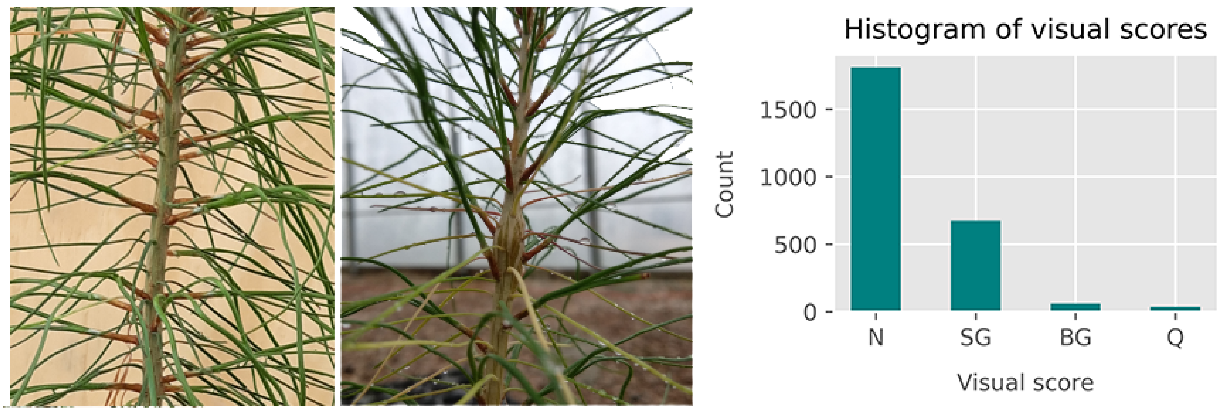
5]. The latter is beneficial in that fungal spores are applied evenly throughout the test population, and disease incidence can be evaluated within six to nine months post-inoculation. The seedlings are visually evaluated for the presence or absence of rust galls (see Figure 2(left)). Rust disease resistance at the family level is determined by the percentage of galled seedlings observed within each family [
6]. However, as described in [
7] with respect to various plant species, visual estimation of disease incidence and severity is highly subjective and prone to human errors, in addition to being a labor-intensive process. Moreover, visual assessment can only be conducted after a period of disease infection when symptoms have sufficiently developed.
An objective and rapid method using imaging technology for disease identification would be beneficial for facilitating the disease screening of loblolly pine seedlings. Hyperspectral imaging, which acquires spatial and spectral information simultaneously, has been successfully employed for the detection of plant disease and stress in multiple plant species [
8,
9,
10,
11]. In these studies, early onset of disease and stress was detected in multiple crops with varying degrees of success. Because of the presence of both spectral and spatial information, hyperspectral imaging provides the opportunity to analyze spectroscopic information at different spatial scales, varying from plant canopy to organs or tissues. This would be beneficial for the assessment of fusiform rust resistance since the disease results in localized symptoms, specifically affecting the stem and branches of young trees.
Based on the location of apparent symptoms, the spectral data from seedling stems can be expected to contain information enabling the successful classification of plants into diseased and non-diseased groups. On the other hand, disease pathogens can often have complex effects on plant physiology and affect the optical properties of multiple plant parts [
12]. This is the reasoning behind the use of spectral data from the entire plant as well as from multiple plant parts, not limited to the part with visual symptoms.
A more controlled approach in data acquisition for disease detection is to collect data only from the plant part that displays disease symptoms. An example of this approach can be found in [
13], where the authors used hyperspectral imaging to detect
Sclerotinia sclerotiorum on four-month-old
Brassica plants by analyzing data from stems stripped of leaves and branches. Data acquired from a targeted method such as this can be expected to increase the accuracy of disease detection models. The sample preparation process, however, decreases imaging throughput and makes repeated image acquisition from the same plants impossible.
The use of top-view hyperspectral images for the detection of fungal infection in
Pinus strobiformis was presented in [
11]. Classification of infection level was based on vigor ratings, and classification accuracy was found to be higher for the samples at the extreme ends of the rating scale. Recently, Lu et al. [
10] used hyperspectral imaging of whole plants to assess the freeze tolerance of loblolly pine seedlings. Partitioning of the seedling image into three longitudinal sections for model development led to improved accuracies compared to the model developed using images of the full-length seedlings. In this study, hyperspectral images of the whole seedlings were collected in situ, and image processing methods were developed to extract spectral data from specific plant parts. To further increase the throughput of the system, multiple seedlings were imaged at a time such that a single hyperspectral image cube contained spectral information from five to seven seedlings.
The selection of regions of interest (ROIs) is a vital step in hyperspectral image analysis since acquired images often contain irrelevant pixels that need to be removed. A common approach is to select one or more image channels that provide suitable contrast for ROI segmentation. This selection can be based on domain knowledge or simple observation. Thresholding or other image processing methods can subsequently be used to obtain segmentation masks. In the case of plant images, vegetation indices such as the normalized difference vegetation index (NDVI) derived from two images at the red and near-infrared wavelength bands are commonly used for the segmentation of vegetation pixels [
14,
15]. While the thresholding of such spectral ratios can be useful for the segmentation of vegetation pixels from the background, the subsequent discrimination of the segmented plant pixels into different classes based on plant parts is a more challenging task. Methods such as the use of an empirically determined wavelength channel [
16], machine learning models based on pixel-wise spectral data [
17], and deep learning models [
18] have been investigated for this purpose.
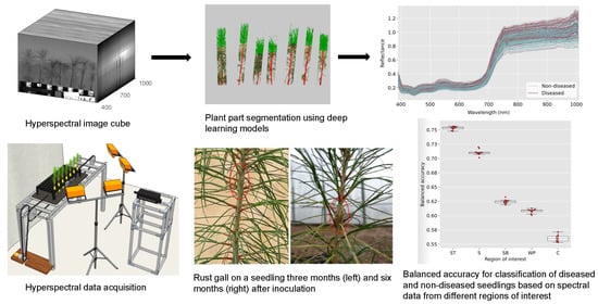
In this study, we first applied a threshold to NDVI images for the segmentation of vegetation pixels. Subsequently, deep learning models based on Convolutional Neural Networks (CNNs) were trained and utilized for the semantic segmentation of different plant parts. We extracted Red–Green–Blue (RGB) images from the hyperspectral image cube and trained a semantic segmentation model to discriminate the stem and foliage of the loblolly pine seedlings. In addition, a deep learning-based object detection model was used for the delineation of individual plants from images containing a row of seedlings. After the extraction of spectral data from plant segments, support vector machine (SVM) classification models were trained for the classification of diseased and non-diseased plants.
This paper presents an innovative method of using hyperspectral imaging technology for the screening of loblolly pine seedlings for fusiform rust disease incidence by using deep learning methods for plant delineation and plant part segmentation. The methods and results presented here are based on the hyperspectral data collected six months after fungal spore inoculation, which corresponds to the typical time for visual assessment of symptoms [
19]. The specific objectives of the current study are as follows:
Development of a hyperspectral image processing pipeline for the extraction of spectral data from specific ROIs in images of loblolly pine seedlings;
Evaluation of SVM classification models for the discrimination of diseased and non-diseased seedlings based on the spectral data from specific ROIs from (1).
Preliminary results leading to this article were previously presented at the 2020 Annual International Meeting of the American Society of Biological and Agricultural Engineers [
20].
2. Materials and Methods
2.1. Plant Materials
The loblolly pine seedlings evaluated in this study were provided by the North Carolina State University Cooperative Tree Improvement Program. The seedling population included a total of 87 seedlots, comprising 84 half-sibling families pollinated with a common pollen mix composed of pollen from 20 unrelated selections, one checklot that consisted of bulked seed from 10 females that were mated with the pollen mix previously described, and two checklots each comprising a single open pollinated family.
Seedlings were sown in May of 2019 at the North Carolina State University, Horticulture Field Laboratory in Raleigh, North Carolina, into Ray Leach Super Cell Cone-tainers (Stuewe and Sons, Inc., Tangent, OR, USA). Two months after sowing, seedlings were organized into replicates. There were 60 replicates, of which 30 replicates were used in this analysis, each with 84 seedlings comprising one seedling per seedlot (incomplete block design). A resolvable row–column incomplete block design was used to maximize the joint occurrence of family in every row and column position across replicates using the CycDesigN software [
21]. Seedlings were subsequently spaced out such that every other cell was occupied (half-tray capacity, equivalent to 49 cells), to increase growing space per seedling and root collar diameter. After spacing, each replicate consisted of two trays, and the row within tray and column within replicate corresponded to the incomplete blocks.
In August 2019, the seedlings were artificially inoculated at the USDA Forest Service Resistance Screening Center (RSC) in Asheville, North Carolina. A broad-based inoculum was used, representing the coastal deployment range of loblolly pine. Inocula were sprayed at a density of 50,000 spores per milliliter using a controlled basidiospores inoculation system, placed in a humidity chamber set for optimal growth with temperatures ideal for fungal infection, then moved to the RSC greenhouses. Three weeks later, the seedlings were transported back to the Horticulture Field Laboratory in Raleigh, NC, USA.
2.2. Hyperspectral Image Acquisition
Hyperspectral scans were collected one week prior to inoculation (mid-August, 2019) and at approximate monthly intervals after inoculation (September 2019 to February 2020). The results presented in this article are based on the hyperspectral images collected in February 2020 from 2521 seedlings included in this experiment. The timing of the data corresponds to approximately six months after inoculation, which is the typical timing for visual assessment in conventional phenotyping.
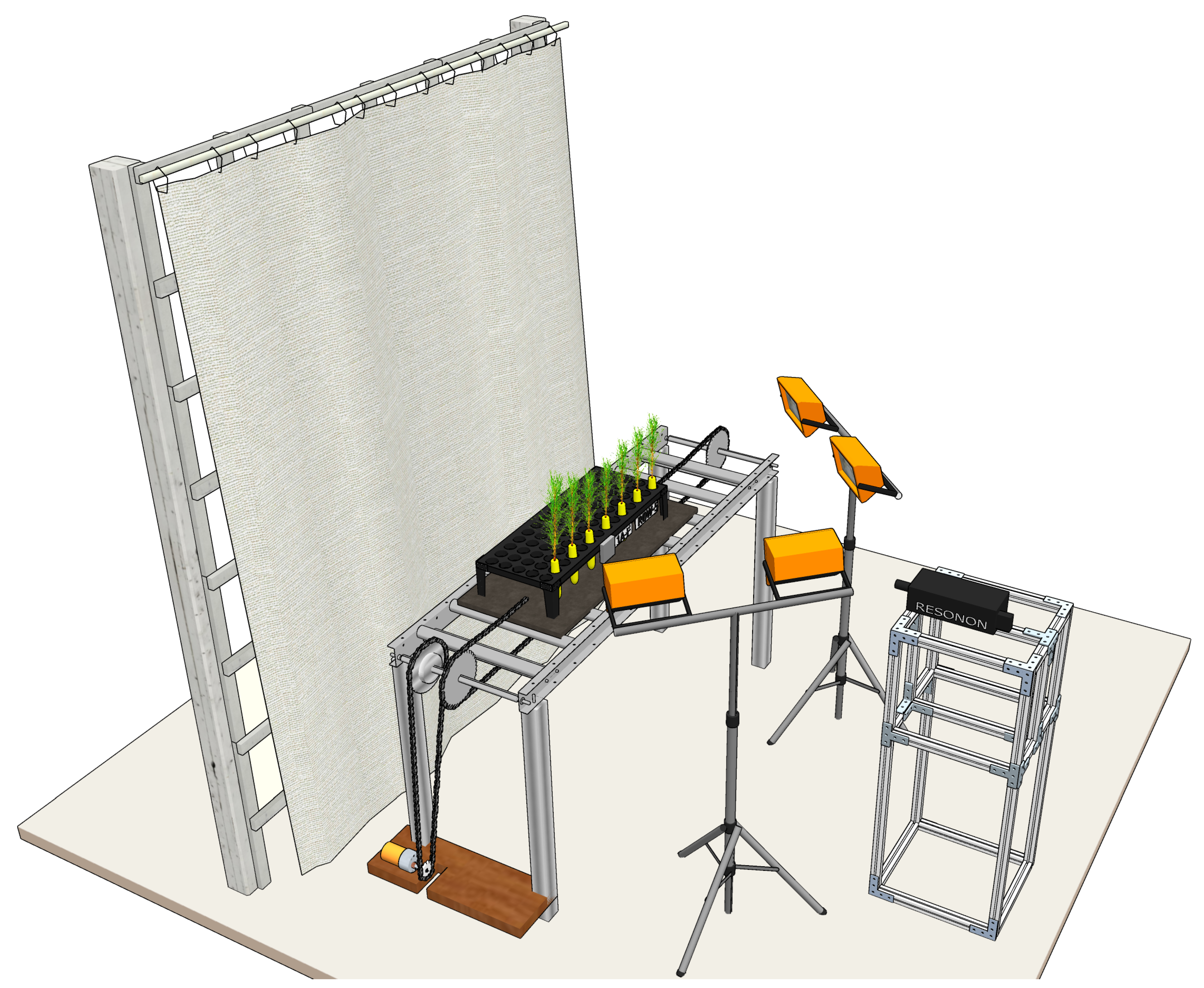
A line scanning hyperspectral imager (Pika XC2, Resonon Inc., Bozeman, MT, USA) was used for the collection of hyperspectral data in the range of 400 to 1000 nm with a spectral resolution of 1.3 nm. The hyperspectral image cubes had the dimensions 1600 × n × 462, where n is the number of line scans used in creating one data cube and 1600 is the number of pixels for each line. The speed of the conveyor stage and the frame rate of the imager were calibrated to ensure an appropriate aspect ratio in the images created. The imager was kept stationary, and a tray loaded with a single row of seedlings was moved across the field of view of the imager using a custom-made conveyor system operated with an electric motor.
The conveyor system was controlled using an Arduino microcontroller that was programmed for forward and reverse motion. The imager was triggered using the bundled software “Spectronon” provided by the manufacturer. A seedling tray was loaded with five to seven seedlings at a time for a side-view scan before being placed on the conveyor board. Halogen lamps were symmetrically placed for additional lighting and a gray cloth was used as a backdrop to facilitate segmentation of plant pixels. A calibration target (SRT-20-020, Labsphere, Inc., North Sutton, NH, USA) with nominal reflectance of 20% was scanned along with the pine seedlings for the standardization of spectral data. A render of the imaging setup is shown in
Figure 1.
2.3. Visual Assessment
Post-inoculation visual scores were used as ground truth data for the classification models and were collected at 6, 26, and 48 weeks post-inoculation. The analysis in this paper is based on the visual assessment conducted at 26 weeks post-inoculation. Based on the presence or absence of rust galls or lesions, seedlings were scored as “diseased”, “questionable”, and “non-diseased”. The seedlings ranked as diseased and non-diseased were the only ones used for the analysis presented in this paper.
Less than 1% of the seedlings (51) were observed to show the early development of rust galls that were not the result of the artificial inoculation but were likely caused by ambient fungal spores given the timing of gall development. The ambient infection was expected since the seedlings were not treated with any fungicides. These galls appeared at the base of the seedlings, whereas the galls caused by the artificial inoculation were observed at the approximate height of the plant-tops at the time of inoculation such that these were always situated on the top half of the stem. This is an expected observation since the succulent tissue amenable to infection by basidiospores is present near the apical meristem at the point of inoculation. The plants with galls at the base of the stem can thus be assumed to have been infected at a date earlier than the date of artificial inoculation, and these plants were also excluded from the discrimination analysis presented in this paper. A histogram of the distribution of seedling scores is shown in
Figure 2.
2.4. Image Processing
2.4.1. Background Removal
Segmentation of plant pixels was carried out by thresholding a normalized difference vegetation index (NDVI) image derived using the two image channels at 705 nm and 750 nm corresponding to the red edge and the near-infrared regions, respectively. This ratio is also referred to as ND705 in the literature; the mathematical relationship used for the calculation is shown in Equation (
1) [
22,
23].
where,
The plant pixels in the NDVI image were segmented from the background by applying an empirically derived, fixed threshold of 0.1. The initial segmentation was refined by removing noise pixels through area opening, where any connected component with fewer than 1000 pixels was filtered out.
2.4.2. Plant Delineation
The separation of image regions corresponding to individual pine seedlings was necessary for the extraction of spectral data associated with each plant. The separation of seedlings was challenging to achieve because of the variation in heights and orientations combined with the slight overlap between the needles from adjacent plants. A reliable method for estimating the number and location of plants in an image was found to be the presence of the Cone-tainers in which the plants were grown. The consistent shape and size of the Cone-tainers made them suitable features for localizing the plant position using computer vision techniques.
For this purpose, RGB images extracted from the hyperspectral image cube were used to train an object detection and localization model. The wavelength bands used for the red, green, and blue bands were, respectively, 640 nm, 550 nm, and 460 nm. For object detection, the Faster RCNN architecture [
24] was selected since it is a general-purpose object detection framework that is computationally efficient and has been shown to perform well in a variety of computer vision tasks. This framework consists of a Fully Convolutional Network (FCN) based on the Region Proposal Network (RPN) that predicts probable image regions containing the object of interest. A pretrained deep CNN is used as the feature extractor before the RPN is deployed in the object detection pipeline. The output of the RPN, which is a set of image regions with an “objectness” score for each region, is used for the extraction of feature vectors that are ultimately used for classification by a fully connected layer. The final output of this model consists of the coordinates of bounding boxes and the probability of an object being contained in each bounding box.
In this study, an implementation of Faster RCNN that is available within the Tensorflow Object Detection API [
25,
26] with inception v2.0 [
27] as the base feature extractor was used for training. A model pretrained with the COCO dataset [
28] was selected in order to take advantage of transfer learning. This model was initially fine-tuned for the detection of pine seedling containers using 25 images with 155 annotated instances of the Cone-tainers in the images. The training was conducted by resizing the images to 50% of their size with a learning rate of 0.0002, and training was stopped after 40,000 steps. This trained model was then used to detect the Cone-tainers in 100 additional images, the detected bounding boxes were manually corrected when necessary, and these 100 images were once again used as training data for training a new model. In this case, the training was stopped after 50,000 steps.
The bounding boxes predicted by the object detection model recognizing the Cone-tainers provided a location for the base of the seedlings, but the seedlings were not always vertically oriented. To ensure a better segmentation of the region occupied by each seedling, the orientation angle of the main stem was estimated by fitting a straight line through the segmented plant pixels after the rudimentary removal of the needles. The color vegetation index [
16,
29] shown in Equation (
2) was calculated and a threshold of 1.9 was used for each pixel.
where
CI is the color vegetation index;
R,
G, and
B are the intensities of the red, green, and blue channels, respectively.
2.4.3. Crown Segmentation
The topmost part of the foliage was segmented out on the basis of the horizontal spread of pixels. Specifically, a horizontal projection or the row-wise sum of non-zero pixels was obtained for the delineated trapezoidal region containing each seedling. The top third section of the segmented plant was taken and the boundary of the crown pixels was determined by finding the most prominent peak in the horizontal projection values. The peak location was determined using the find_peaks function provided by the Python library SciPy [
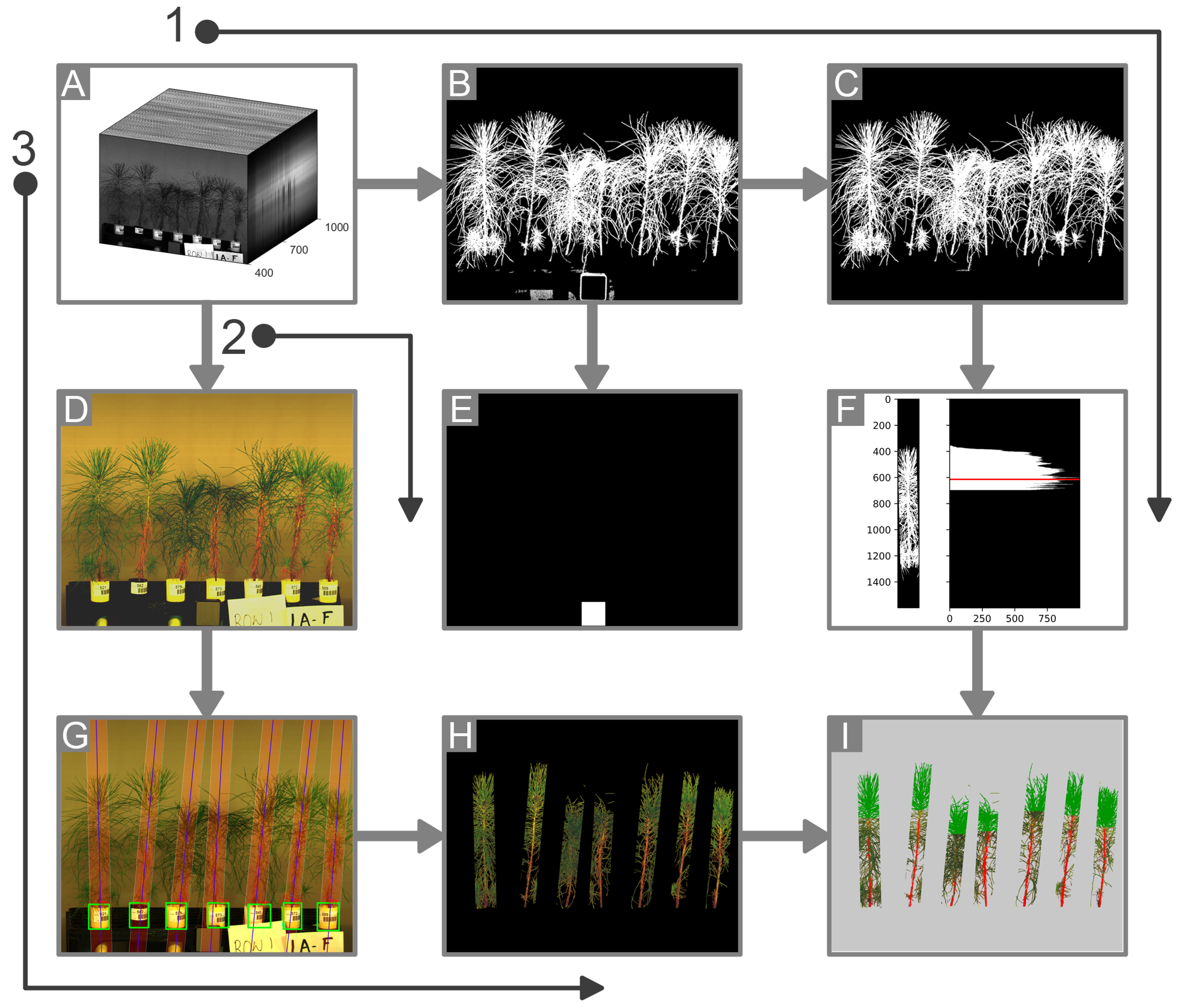
30]. The image processing pipeline is shown in
Figure 3.
2.4.4. Stem Segmentation
Stem segmentation was carried out by using the DeepLabv3+, which is an iteration of the DeepLab CNN model for semantic segmentation [
31]. DeepLabv3+ uses an encoder–decoder architecture, where the encoder module consists of the Xception model [
32] as the feature extractor. The DeepLab family of segmentation models makes use of atrous or dilated convolution, which uses convolution kernels with gaps between values. This leads to a larger field of view for a kernel without adding to the computational cost that would result from additional parameters in the case of the standard convolution operation. DeepLabv3+ specifically uses Atrous Spatial Pyramid Pooling (ASPP) to encode the features at different spatial scales while using a decoder module for precise delineation of boundaries. The encoder creates a feature map that is a fraction of the size of the input image, and the decoder comes into play for the restoration of the feature map to the original size of the image. The decoder module of the DeepLabv3+ model uses bilinear interpolation for the upsampling combined with convolution operations. The reader is referred to [
31] for details on the model architecture; the default model available from the Tensorflow model repository [
33] was used with the custom training dataset in this study.
To prepare the training data, a rudimentary stem segmentation was conducted by the thresholding process described in
Section 2.4.2. The result of this segmentation was manually corrected using the Image Labeler app included with the Computer Vision Toolbox in Matlab 2019a (Mathworks, Inc., Natick, MA, USA). This approach led to a reduction in the labeling effort since the rudimentary label map was created by the algorithmic approach, and the manual work was limited to the correction of this label map.
The accuracy of the stem segmentation by DeepLabv3+ was assessed using pixel accuracy and mean Intersection over Union (mIoU). Pixel accuracy can be defined as the ratio of the number of correctly classified pixels to the total number of pixels. mIoU is a widely used metric for the evaluation of semantic segmentation models, and it is more robust compared to pixel accuracy in the case of imbalanced class sizes [
34]. The mIOU was calculated by taking the average of the Intersection over Union (IoU) values across different classes. The equations used for the calculation of these metrics are shown in Equations (
3) and (
4).
where,
2.4.5. Segmentation of the Reflectance Standard
An empirical method for the segmentation of the calibration panel was determined based on the spectral properties of the material used to enclose the standard material. The plastic casing was found to be consistently segmented out when using the NDVI thresholding described for the segmentation of the plant pixels in
Section 2.4.1. As a result, a group of pixels resembling a square shape was segmented out when thresholding for the plant pixels. This information was used to segment out the pixels of the reflectance standard. Since the same NDVI image could be used for plant segmentation as well as for the segmentation of the calibration panel, this led to a reduction in computation and an increase in the throughput of the segmentation process. The steps involved in the segmentation of the calibration panel can be seen in
Figure 3. Other approaches could be used for the segmentation of the reflectance standard—for example, by using the spectral properties of the Spectralon material available from the manufacturer’s calibration. The approach used in this study was adopted solely for convenience and speed of processing.
2.5. Spectral Pre-Processing
The spectra from the pixels in each segmented ROI were averaged to obtain a mean spectrum of raw intensity values. The mean spectrum of the Spectralon reflectance standard (SRT-20-020, Labsphere Inc., North Sutton, NH, USA) was first used for the radiometric correction of raw spectra from the ROIs. The calibration data comprised the reflectance values from 250 nm to 2500 nm for the reflectance standard. The values between 400 nm and 1000 nm relevant for this study were retrieved and linear interpolation was used to obtain reflectance values for each wavelength band in the hyperspectral data of the seedlings. The relationship used for this calculation is shown in Equation (
5).
where,
Reflectance spectrum for the plant region of interest (ROI);
Mean raw intensity (i.e., digital number) values for the plant ROI;
Mean raw intensity values for the Spectralon standard;
Reflectance values for the Spectralon standard provided by the manufacturer.
Since the extracted dataset included noisy spectra, the Local Outlier Factor [
35] with a neighbor size of 10 was used for the removal of outliers. Next, a Savitzky–Golay filter with a window size of 11 and polynomial order 3 was used for spectral smoothing. The window size and polynomial order were selected for efficient smoothing as well as for higher accuracy of the downstream classification models. The dimension of the spectral data was conserved by fitting the polynomial of order 3 to the last window to calculate values for the padded signal. The savgol_filter function provided by the Python library SciPy [
30] was used for the implementation.
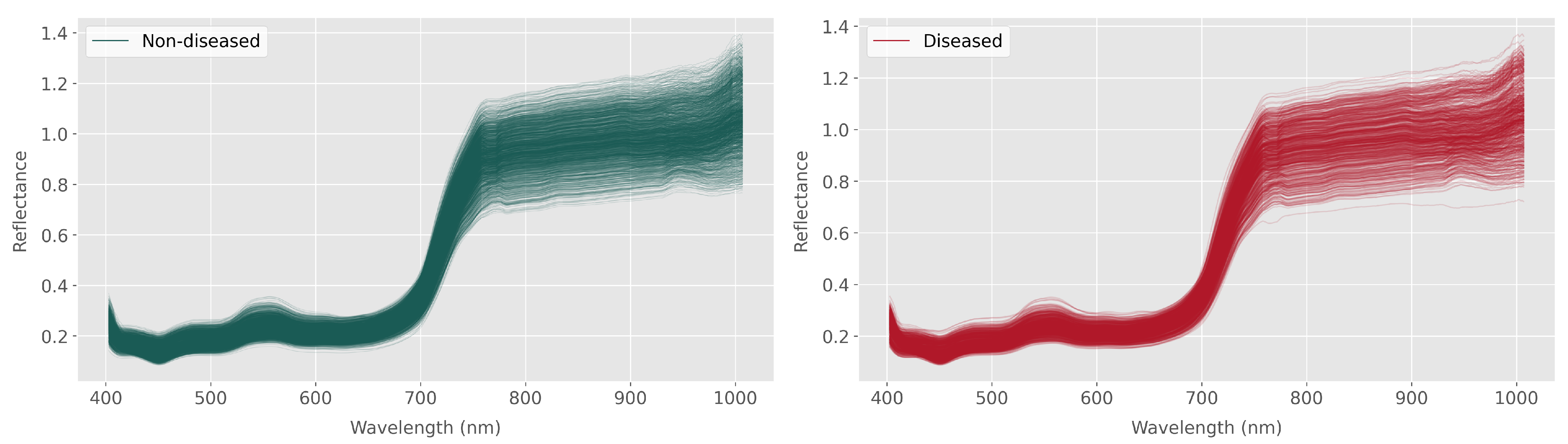
Figure 4 shows the processed spectra for the whole plant, with the diseased and non-diseased seedlings differentiated in the figure. The curves represent 1708 non-diseased plants and 653 diseased plants based on the visual scoring.
2.6. Classification Models
After the processed spectra from each region of interest have been extracted, the discriminant analysis with the extracted spectral data is reduced to the problem of multivariate classification. However, the dataset being imbalanced across the diseased and non-diseased groups (see
Figure 2) made it unsuitable for the direct implementation of a general classification algorithm that does not consider class imbalance. Several techniques are available for conducting discrimination analysis with imbalanced datasets, including the use of cost-sensitive learning techniques, and oversampling of the minority class or undersampling of the majority class [
36,
37]. A widely used method of oversampling coupled with the synthetic generation of data for the minority class is the Synthetic Minority Oversampling Technique (SMOTE) proposed in [
38]. SMOTE was implemented for our dataset using the imbalanced-learn library in Python [
39].
As part of the investigation into discrimination using the extracted spectral data, support vector machine (SVM) models with a linear kernel were used to classify seedlings into diseased and non-diseased groups. A linear kernel was the preferred choice because of the large number of features, as recommended in [
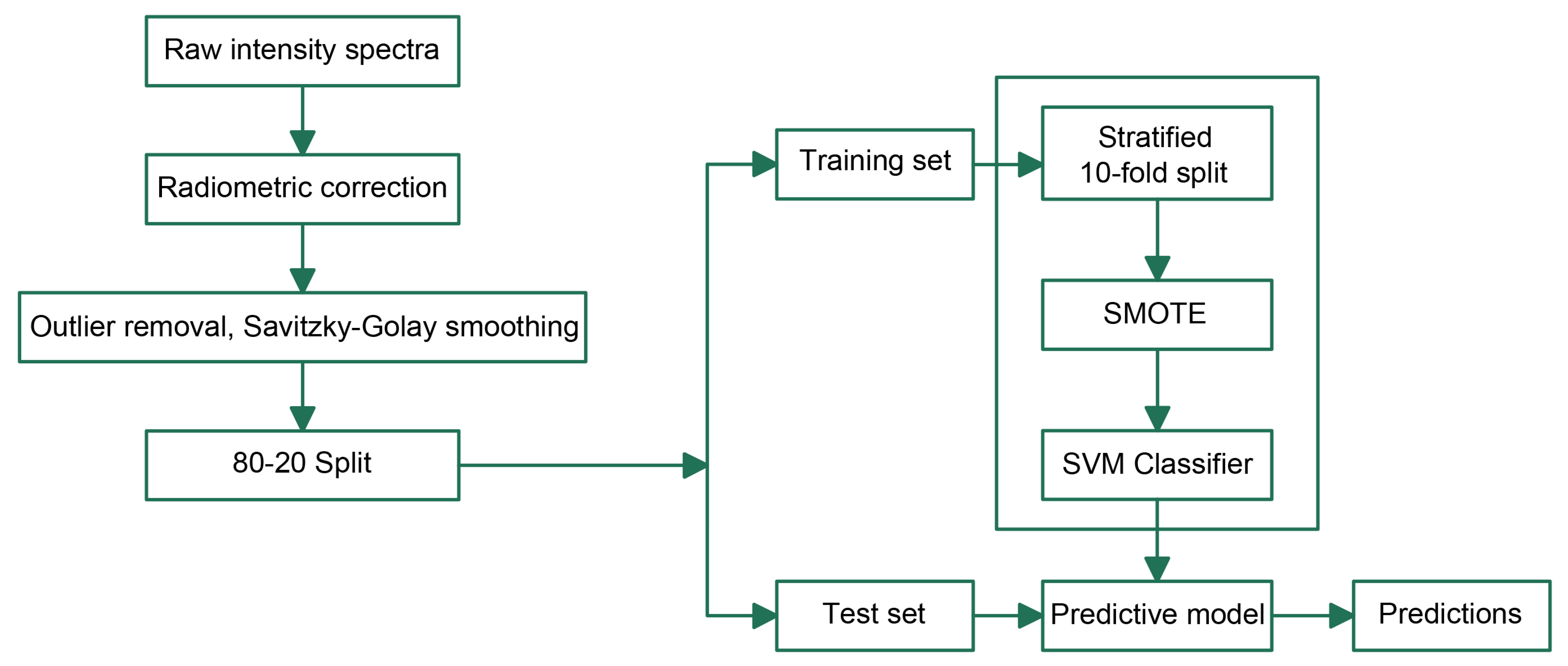
40]. A grid search with 10-fold cross-validation was used to find the optimum value of the regularization parameter C, where the vector used for the search space was [0.1, 1, 10, 100, 200, 300, 400, 500, 600, 700, 800, 900, 1000, 10000]. The values for the search were used based on preliminary test runs with the training set. The flowchart in
Figure 5 shows the steps followed in the SVM modeling combined with SMOTE oversampling for the classification of diseased and non-diseased groups. The data were first randomly split into a training set (80%) and test set (20%), the training was conducted with 10-fold cross-validation incorporating SMOTE oversampling, and, finally, the selected model was applied to the test set for prediction.
Balanced accuracy values were calculated as evaluation metrics for the discrimination models. Balanced accuracy is defined as the average of the proportion of correctly classified samples across all classes. In this study, the balanced accuracy of a prediction model provides the average of the accuracy in classification for the diseased and the non-diseased groups. Due to the unbalanced number of samples across the two classes, this is a more robust and reliable measure of accuracy compared to the simple proportion of correctly classified samples. It is also a commonly used metric for the evaluation of plant disease detection models [
41,
42]. Ten values of balanced accuracy were calculated (with 10-fold cross-validation in each run) for each ROI and a one-way analysis of variance (ANOVA) followed by Tukey’s honestly significant difference (HSD) tests at 5% significance level (
) were conducted to evaluate whether a statistically significant difference existed among the evaluation metrics for the different ROIs.
where,
TP = True positive rate;
TN = True negative rate.
A commonly used evaluation tool for diagnostic tests is the receiver operating characteristic (ROC) curve [
43,
44]. The ROC curve is the graph of the true positive rate against the false positive rate. The upper left corner of this plot, representing a 100% true positive rate and a 0% false positive rate, is thus the plot for an ideal classifier. The line inclined at 45º to the positive X-axis, on the other hand, represents a classifier without any power of discrimination. An ROC plot was created, and the area under the curve (AUC) was observed for the optimum ROI selected from the comparison of balanced accuracies. AUC values from the ROC curve are often used as metrics for the evaluation and comparison of binary classifiers [
45]. An AUC of 0.5 represents a model equivalent to a random guess, whereas a higher value of AUC represents greater discrimination ability. The use of ROC analysis enables the selection of an appropriate threshold with a desired tradeoff between the true positive rate and true negative rate of a diagnostic test, also referred to as the sensitivity and specificity, respectively. ROC analysis can be especially useful for experiments in plant phenotyping since these experiments are often aimed at finding the best- or the worst-performing samples in the population, and the threshold for discrimination can be adjusted accordingly for the optimum sensitivity or specificity. AUC values have been often used as a metric for the evaluation of plant disease detection algorithms, especially in the case of imbalanced datasets [
46,
47].
4. Discussion
In this article, we present a deep learning-based approach for the segmentation of specific regions of interest in Vis–NIR images of loblolly pine seedlings followed by a study in disease discrimination using hyperspectral data extracted from these ROIs. The segmentation of ROIs based on the features extracted from one or more image channels or their combinations is a common technique that has been used in studies using hyperspectral imaging. In addition to the use of traditional techniques of segmentation, such as the red-edge NDVI, the use of the visible section of Vis–NIR images to leverage the power of pretrained deep learning models was found to be a promising approach for the extraction of complex ROIs.
Experiments in plant phenotyping of large populations using hyperspectral imaging have a trade-off between the throughput of data acquisition and the complexity of data processing. The collection of data from well-prepared samples in a controlled environment is ideal for analysis but suffers from low throughput of acquisition. The current study only moderately controlled the data acquisition in a greenhouse environment for the sake of increasing throughput. Images were acquired under ambient lighting with supplemental halogen lamps when necessary, and multiple plants were imaged together in greenhouse trays. As a result, the subsequent processing of the images required multiple steps for the processing and extraction of relevant information. Since a data processing pipeline, once developed, can be repeatedly used for subsequent datasets, we consider a more involved data processing pipeline preferable to the low-throughput acquisition of data.
Morphological symptoms of fusiform rust are visible in the form of galls and lesions on the stem, which makes the detection of symptoms in the images non-trivial. The logical choice of ROI for the acquisition of spectral data was the stem; however, we conducted the study using multiple regions of interest for two reasons:
Successful discrimination using the spectral data from the whole plant would increase the efficiency of the data acquisition while also decreasing the effort required in subsequent image processing;
Spectral signatures in the NIR region could lead to successful discrimination using spectral data from non-stem pixels irrespective of the location of visible symptoms.
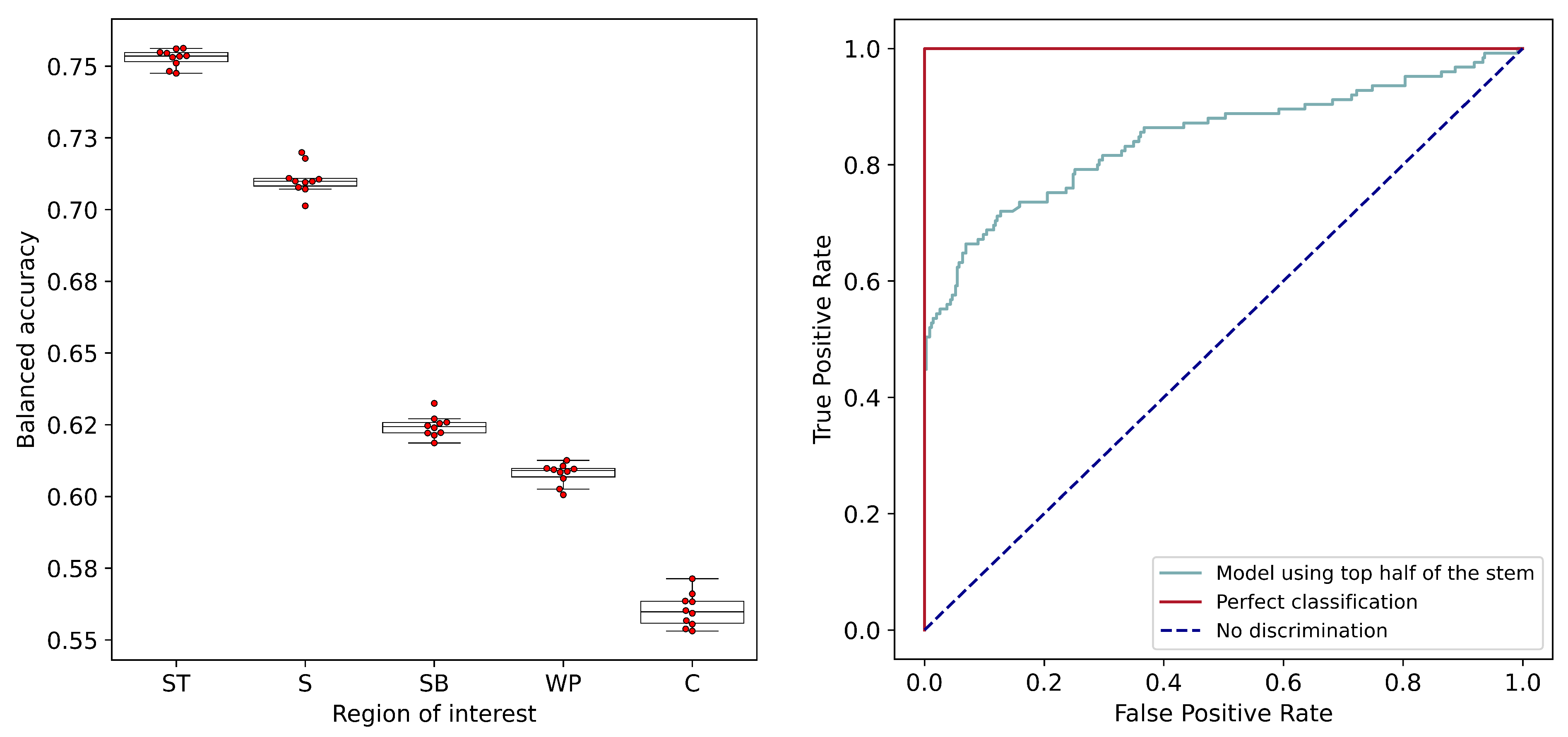
The comparison of discrimination models using data from multiple ROIs indicated that the top half of the stem is the optimum ROI, thus establishing that the region of the visible symptoms should indeed be the ROI of choice. With this conclusion, the image processing pipeline developed for the segmentation of stem pixels will be useful for future experiments and analysis.
When using deep learning models, the labeling of a large number of images can require significant time and effort, especially in the case of pixel-wise labeling for semantic segmentation models. A semi-supervised labeling method was used in this study, where an imperfect but quick segmentation was achieved using a color index to remove most of the non-stem pixels. The “correction” of this imperfect stem segmentation was less labor-intensive compared to the manual labeling of the images.
The discrimination model using the spectral data from the top half of the stem achieved a balanced accuracy rate of 77% and an AUC of 0.83 from the ROC curve. While these values indicate the presence of promising discriminatory power, it is noted that better accuracies are possible and desirable.
One of the conclusions that can be derived from this study is that a more controlled environment for data acquisition, with the targeted imaging of the top half of the stem, would increase the potential for creating more accurate models. A study using the controlled acquisition of hyperspectral images from the infected stem, similar to [
13], would be informative for the establishment of a best-case scenario. Since the signals associated with the disease interact with biotic and abiotic factors, the accuracy and reliability of the detection method can be expected to increase with an increase in the level of control associated with data acquisition.
The use of automated phenotyping platforms with the capability of longitudinal data acquisition in a controlled environment is a promising tool for disease discrimination. As noted by [
48], these platforms enable the acquisition of multi-dimensional traits, including changes in physiology and morphology. While the need for visual screening persists for accuracy and reliability [
49], the importance of sensor-based discrimination approaches can be expected to increase in the future. In addition to the improvements possible via data acquisition methods, the selection of specific wavelength values with sufficient information for disease detection is another possible avenue of research [
42,
50]. The reduction of high-dimensional hyperspectral data to spectral indices or spectral signatures derived from a few wavelengths decreases the complexity of data analysis and can also enable the use of less expensive multispectral cameras for data acquisition.
This study represents an initial proof-of-concept for high-throughput fusiform rust disease screening in loblolly pine. Hyperspectral imaging promises several advantages over human-based visual evaluation in terms of its objectivity and amenability to automation, and it can potentially be integrated into a tree improvement selection strategy. In this study, an encouraging level of discriminatory power was achieved using the spectral data from the top half of the stem. The balanced accuracy rate of 77% and an AUC of 0.83 from the ROC curve could be further improved by increasing the level of control in data acquisition and by investigating a wider range of wavelength values. Following further optimization of the scanning environment, there will be the opportunity to evaluate the rate and severity of disease expression caused by the artificial inoculation of seedlings. Family differences could be assessed not solely based on the presence or absence of rust galls but also the rate and severity of gall development. Additionally, hyperspectral data can enable the early detection of disease before the visual symptoms become apparent; this would reduce the time and expense associated with the conventional screening process.


 ,
, 


