Fine-Grained Large-Scale Vulnerable Communities Mapping via Satellite Imagery and Population Census Using Deep Learning

Abstract

One of the challenges in the fight against poverty is the precise localization and assessment of vulnerable communities’ sprawl. The characterization of vulnerability is traditionally accomplished using nationwide census exercises, a burdensome process that requires field visits by trained personnel. Unfortunately, most countrywide censuses exercises are conducted only sporadically, making it difficult to track the short-term effect of policies to reduce poverty. This paper introduces a definition of vulnerability following UN-Habitat criteria, assesses different CNN machine learning architectures, and establishes a mapping between satellite images and survey data. Starting with the information corresponding to the 2,178,508 residential blocks recorded in the 2010 Mexican census and multispectral Landsat-7 images, multiple CNN architectures are explored. The best performance is obtained with EfficientNet-B3 achieving an area under the ROC and Precision-Recall curves of 0.9421 and 0.9457, respectively. This article shows that publicly available information, in the form of census data and satellite images, along with standard CNN architectures, may be employed as a stepping stone for the countrywide characterization of vulnerability at the residential block level.

1. Introduction

Historical statistics indicate that the poverty rate is steadily receding worldwide [1]. Take, for instance, extreme global poverty. In 1990, 1895 million people had an income of less than USD 1.90 at constant 2011 purchasing power parity prices (PPP). In 2015, this value was reduced to 736 million people [2], i.e., an estimated 122,100 individuals abandoned extreme poverty around the world each day during that period. Although the poverty rate is receding, global income inequality may be on the rise in some countries [3]. For instance, in the U.S., the top 1% holds 40% of the total net wealth, as opposed to 25% in the 1980 [4]. Furthermore, the poverty rate is unevenly distributed worldwide, with Sub-Saharan Africa affected at a much larger scale than the world in general. For example, in 2016, 95.5% of the U.S. population received as income USD 10 or more daily, versus 31.3% of Mexican people. This income level translates to 16.36 million individuals in the U.S. and 88.85 million in Mexico living below the international poverty line of USD 10 daily [5]. Poverty means families are going hungry, children have little or no access to education, reduced services (e.g., electrical power, drinking water), and poor health [6]. Communities of people living in poverty are vulnerable to physical factors and social exploitation. Building on the principle of Leave No One Behind, the U.N. adopted the 2030 Agenda for Sustainable Development, which included eliminating extreme poverty as its primary goal.

Critical steps in combating poverty include identifying, assessing, and tracking the sprawl of affected communities. These steps are necessary to plan socio-economic interventions and evaluate their efficacy. For example, periodic national census exercises are designed to grab an instant photo of a country’s status. Unfortunately, nationwide censuses require considerable effort and take place only sporadically, e.g., every ten years in Mexico. A better and more economical approach is necessary to generate timely information on affected communities’ location and poverty status. Several technological trends can reduce the cost of this process and produce reliable, up-to-date data. These technologies rely on sensory information from space [7] as it is becoming increasingly abundant, precise, and cheap to obtain. Furthermore, recent advances in machine learning techniques make it possible to extract relevant sensory data indicators, informing and guiding policymakers.

Thus, there has been a considerable interest on mapping vulnerable regions from remote sensing, particularly employing the images provided by the satellites LandSat [8,9], Sentinel-2 [10,11], QuickBird-2 [11,12], TerraSAR-X [12,13], Pleiades [14], and the National Oceanic and Atmospheric Administration (NOAA) Defense Meteorological Satellite Program (DMSP) Operational Linescan System (OLS) [15,16,17,18,19,20]. Both high-resolution [10,12,14] and low-resolution [10,11,15,16,17] images have been considered in rural [9] and urban areas in multispectral [9,10,17], Synthetic Aperture Radar (SAR) [11,13], and color [19,21] images. Multiple machine learning methods including traditional [8,12,16,18,22] approaches such as Random Forest (RF), gradient boosting, Support Vector Machines (SVM), and modern techniques [11,13,14,19,21,23,24] such as Convolutional Neural Networks (CNNs) and Recurrent Neural Networks (RNNs) have been deployed. Some open-source code has been made available to the research community [25]. The scope of assessing vulnerability scales up from the city level [18], to the country level [26], and to the many countries level [15,25]. A critical issue that remains to be explored, which is the object of this paper, is developing techniques for countrywide assessment of vulnerability at the residential block level using the UN-habitat criteria [27] and census data. In the process, we evaluate different CNN architectures to establish an optimal mapping between multispectral images and vulnerability reference values. Moreover, the time seems ripe for implementing a solution for assessing and fine-grained tracking of vulnerable areas at a countrywide level to support policy decision-making.

According to Weeks et al. [28], few attempts had been made to establish an index to define vulnerability beyond the dichotomy slums/non-slums. In their work, Weeks et al. propose an index for a slum based on the characteristics described by UN-Habitat [27], which they call Slum Severity Index (SSI). Patel et al. [29] are the first researchers to report the use of the SSI using microdata from the census as ground truth based on satellite imagery. This paper extends these efforts by introducing a method for the fine-grained assessment of vulnerable community sprawls using multispectral satellite imagery and ground truth data obtained from censuses using deep learning techniques (see Figure 1). The contributions of this paper include the following:

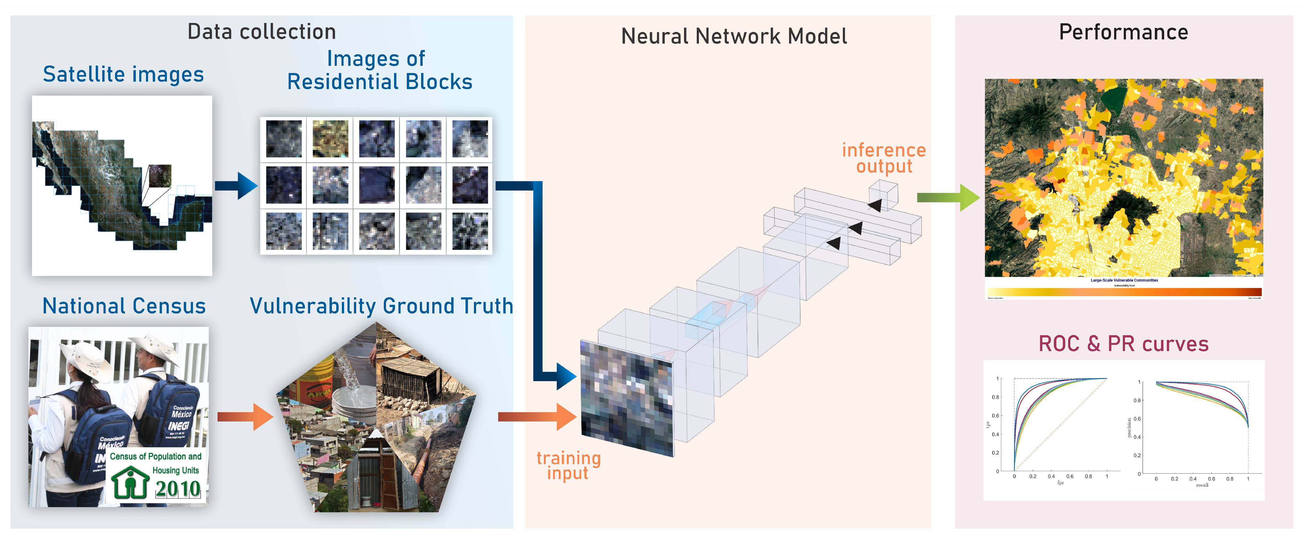
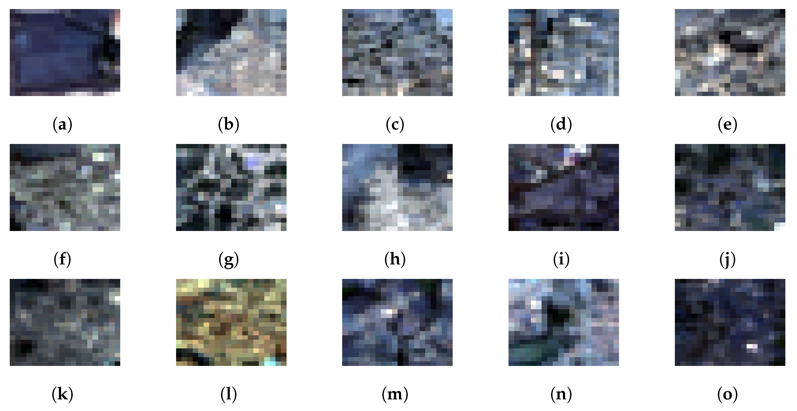
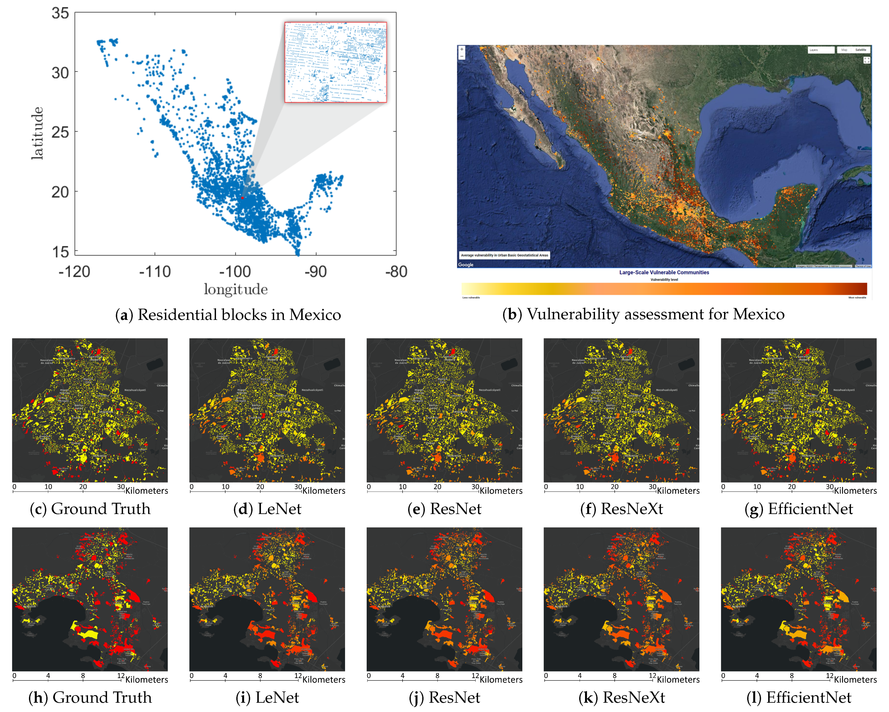
• A nationwide assessment of settlements’ vulnerability for Mexico is conducted at the residential block level.
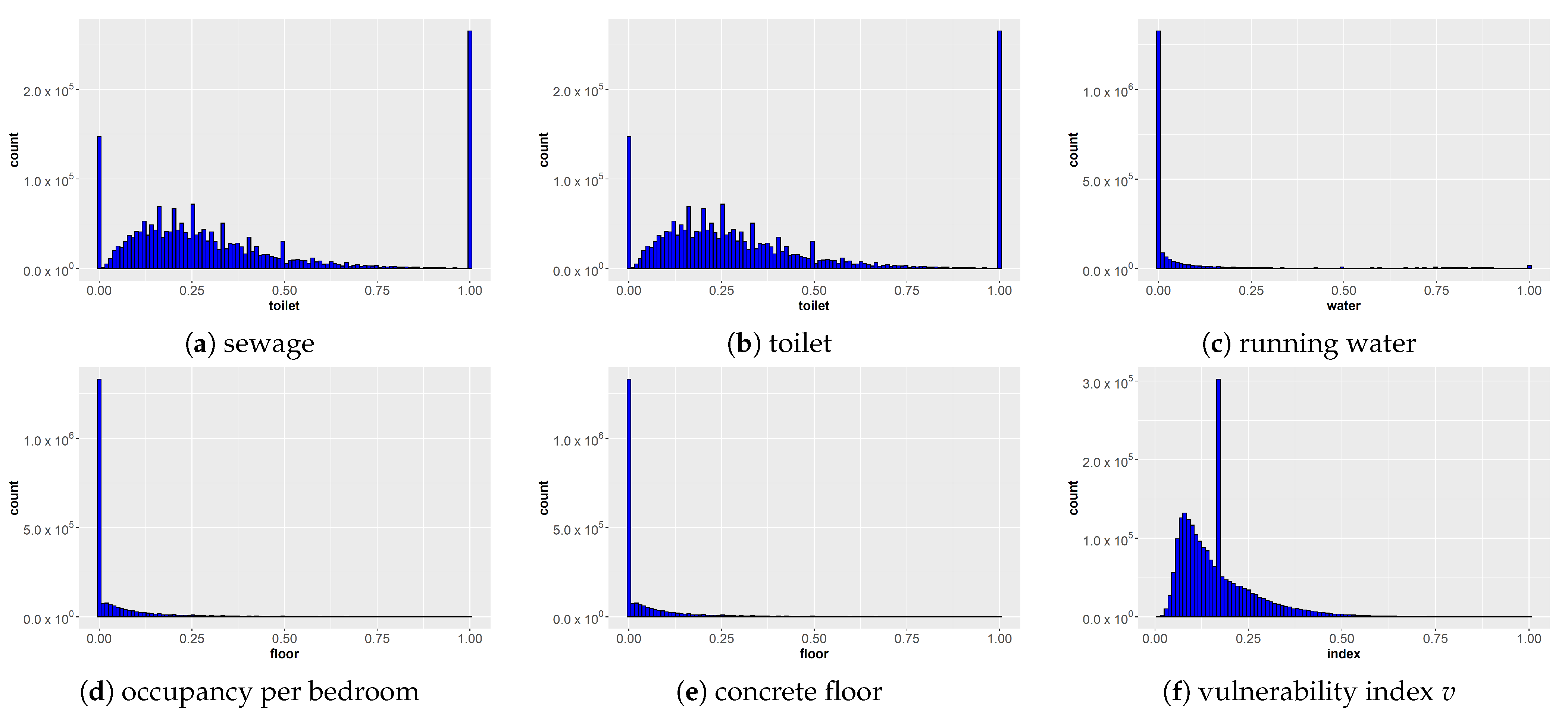
• An alternative vulnerability indicator is developed using the UN-Habitat factors related to settlements [27].
• Using data composed of hundreds of thousands of records, different convolutional neural network (CNN) architectures are assessed in the task of mapping satellite images to the vulnerability index.
• The computer code for this project is made available to the research community. This should permit the evaluation of this work and serve as a stepping stone for further progress in the field.

The rest of the paper is organized as follows. The next section describes an approach to measuring vulnerability using the UN-habitat characteristics and presents a strategy to assess vulnerability using satellite images and a CNN is described. Section 3 describes the results of testing the approach described in the previous section. In particular, it is shown that CNNs are useful for extracting meaningful features, and the performance of these architectures is assessed. Section 4 presents a discussion on the relevance of the results in the context of the related work. The paper concludes with a summary of the findings and provides recommendations for future research.

2. Materials and Methods

In this approach, learning involves the construction of an automatic inference mechanism mapping satellite images to reference values representing a vulnerability index. This section details how we address these issues.

2.1. Characterizing Vulnerability

Vulnerability is an elusive term, often bringing to mind crowded informal settlements without access to essential services. UN-Habitat suggests that an operational definition of a slum should include [27]: (a) inadequate access to safe water, (b) inadequate access to sanitation and other infrastructure, (c) poor structural quality of housing, (d) overcrowding, and (e) insecure residential status. Recently, Roy et al. [22] proposed the Slum Severity Index (SSI) to blend these aspects of vulnerability. Agglomerating per residential block, they defined the SSI employing the average number of persons per room ($x_o$), the proportion of houses without sewage ($x_s$) and toilets ($x_t$), the proportion of dwellings with a dirt floor and temporary structures ($x_f$), and the proportion of homes lacking piped and public water ($x_w$). They then obtained the SSI from the projection of the centered reference values $\mathbf{x}-\mu ={(x_o,x_s,x_f,x_w)}^T-\mu$ on the axis of maximum variability, i.e., the SSI corresponds to the projection of the reference values on the first principal component of the centered observation matrix.

PCA maintains the sensibility of other optimization approaches where the underlying assumption is that the differences are normally distributed and therefore affected by outliers’ presence. Another issue with PCA is that each new axis represents a certain amount of the information available, assuming a representation where the first component points in the direction of maximum variability, and then subsequent ones point in directions orthogonal to the previous ones. Under this interpretation, the singular values provide a proxy for the information I expressed by the first l components. PCA works best when there is a linear relationship between the variables. However, our dataset (see Figure 2) may not hold up that assumption. Furthermore, reference values in this dataset, such as the occupancy per bedroom, may have a long tail, which in practice makes it hard for PCA techniques to provide consistent results as it tries to interpret as Gaussians the distribution of differences between the dataset and its low-rank decomposition.

Avoiding the sensibility of PCA and considering the distribution in this dataset (see Figure 2a–e), an alternative to express vulnerability is developed as follows. First, in this dataset, the reference values range between zero and one, except for the occupancy $x_o$, which has values larger or equal to zero without a pre-defined upper bound. In this case, a possible solution may be to threshold and normalize the occupancy distribution with a constant ${\tau }_o$ as ${\widehat{x}}_o=min({\tau }_o,x_o)/{\tau }_o$. Let the unitary vector ${\widehat{\mathbf{x}}}_i=(x_s,x_t,x_w,{\widehat{x}}_o,x_f)/\sqrt{5}$ describe the content of the dataset for data sample i and the weights vector ${\mathbf{w}}^T=(w_s,w_t,w_w,w_o,w_f)$ describing the relative reference values’ importance. Vulnerability is measured using population responses related to the UN-Habitat criteria [27] obtained from a census using the following procedure. First, from an extensive dataset collected from a nationwide census, the vectors ${\widehat{\mathbf{x}}}_i$ for $i\in \{1,\dots ,n\}$ representing the reference values for the predictors and corresponding to the n data samples are considered. The proposed vulnerability index (see Figure 2f) corresponds to the expression

$$v_i=\frac{{\mathbf{w}}^T}{\mid \mid \mathbf{w}\mid \mid }{\widehat{\mathbf{x}}}_i,$$

(1)

where $\mid \mid \mathbf{w}\mid \mid$ represents the norm of $\mathbf{w}$, the weights associated to each of the reference values. The reference classes can be obtained using

$$\mathcal{C}\left({\widehat{\mathbf{x}}}_i\right)=\left\{\begin{array}{cc}\mathrm{vulnerable}\hfill & if v_i\ge {\tau }_v,\hfill \\ \mathrm{non-vulnerable}\hfill & \mathrm{otherwise},\hfill \end{array}\right.$$

(2)

where ${\tau }_v$ expresses the threshold after which the residential block is considered vulnerable assuming that the weights are equal, when at least one of the reference values is one, ${\tau }_v\ge 0.2$.

2.2. Setup

This dataset consists of 2,178,508 records, corresponding to the residential blocks for Mexico obtained during the 2010 census [30] (see Figure 3). The census contains an aggregate of the reference values of interest collected at each house in a residential block. Following a policy to keep citizens’ privacy, the public census only contains residential blocks with more than five houses. The resulting distribution of values is nonetheless singular (see Figure 2). About 60.23%, 6.75%, 59.81%, and 60.49% have (their value is zero) and 0.43%, 12.16%, 0.88%, and 0.13% do not have (their value is one) sewage, toilets, running water, and concrete floors, respectively. Additionally, for 99.54% of the records, the average occupancy is smaller than three, i.e., only 9834 residential blocks have an average occupancy larger than three. The threshold at ${\tau }_v=0.2$ distinguishes between 853,583 and 1,324,925 records corresponding to the vulnerable and non-vulnerable classes, respectively. For the experiments, a balanced classification problem was created by subsampling 853,583 non-vulnerable records at random. Under the assumption of uniform weights, this threshold may indicate that each dwelling belonging to a particular block lacks an essential service or its rooms are overcrowded.

To run the algorithms, an Exxact server with one Titan-X Pascal GPU was employed. The computer programs extract the geo-location for each residential block using publicly available data [30]. The programs then downloaded the corresponding 600 m × 600 m image patches of the blue (450–515 nm), green (525–605 nm), red (630–690 nm), near-infrared (775–900 nm), SW1 (short wavelength infrared) (1550–1750 nm), and SW2 (2080–2350 nm) Landsat-7 bands for the same year from INEGI (Instituto Nacional de Estadística y Geografía) [31]. Note that the first three and second three bands correspond to the visible $\mathcal{V}$ and infrared parts of the electromagnetic spectrum. Landsat-7 is a helio-synchronous satellite with a repeat interval of 16 days that orbits the Earth at a nominal altitude of 705 km. INEGI generates these images with the geomedian [32] from those captured between 1 January and 31 December 2010. Although Landsat-7 has a resolution of 30 m/pixel, corresponding to image patches of 20 × 20 pixels, the image were resized as required by the architecture under consideration using bicubic interpolation.

2.3. Selecting a Learning Architecture

Given their capacity to extract high-level features, CNNs are employed to construct the map between satellite image patches and the vulnerability reference value. Functionally, a CNN [33] includes convolution operations that transform the input data with the application of data-driven operators. Researchers, such as Li et al. [34], have concluded that the layers extract more abstract features subsequently, starting from edges, corners, and representations generalizing the pattern sought. In each layer, a CNN applies a linear operator to the inputs. To express nonlinearities, one applies activation functions to generate each layer’s outputs. In most cases, one feeds the features developed by the convolutional layers to a fully connected layer. Eventually, the aim is to represent for regression or discriminate for classification, the resulting transformed data with hyperplanes in the last layer. The selected architectures were chosen based on the following criteria: Performance in the ImageNet benchmark [35], availability of ImageNet pre-trained weights in the Tensorflow applications repository [36], and the capability of the target computing resources. Based on these criteria, the CNN architectures selected included ResNet [37], ResNeXt [21], and EfficientNet [38]. In addition, a baseline was established with LeNet-5 [39]. Other popular strategies may be pursued, including the employment of Inception-like architectures [40] or Generative Adversarial Networks (GAN) [41]. The former type of approaches was left for further consideration as we are including ResNext, an architecture that includes the Inception capabilities to analyze features at variable scales. Furthermore, as Perez et al. [42] noted, GANs are most useful in the classification of vulnerable settlements when the references are sparse. In this study, the dense reference values available in the census is complemented with the employment of a high-performance classifier, which itself could be part of the GAN architecture definition in the discriminant.

LeNet [39]. LeNet is used to establish a baseline for comparison. Its introduction with a solid performance on MNIST, consisting of a 28 × 28 pixels dataset of digits, makes it a natural choice for the small image patches in the dataset. This CNN consists of a first part with convolutional layers and a second part with fully connected layers. The convolutional stage has three convolutional layers, where the first two are followed by sampling summarizing layers. Next, the pooling layer reduces the features in each dimension by half. Finally, the fully connected layers lead to the classification.

ResNet [37]. This CNN still shows a strong performance in a wide variety of computer vision and pattern recognition tasks. The ResNet paradigm implements in its architectures the concept of skip connections. That is, suppose that as an input $\mathbf{x}$ passes through a set of layers, it is transformed into $\mathcal{F}\left(\mathbf{x}\right)$. In skip connections, $\mathbf{x}$ joins $\mathcal{F}\left(\mathbf{x}\right)$ to compute $\mathcal{H}\left(\mathbf{x}\right)=\mathcal{F}\left(\mathbf{x}\right)+\mathbf{x}$. In practice, it means that if the overall underlying mapping between input and output is $\mathcal{H}\left(\mathbf{x}\right)$, the machine learns in $\mathcal{F}\left(\mathbf{x}\right)$ the residual $\mathcal{H}\left(\mathbf{x}\right)-\mathbf{x}$. This configuration addresses the degradation problem, i.e., the observation that a deeper network should not generate a higher learning error than a shallower architecture, when in fact, it does. He et al. [37] showed that residual networks can be constructed deeper, are easier to optimize, and gain accuracy from increasing depths.

ResNeXt [21]. ResNeXt implements topologies that split the input into C low dimensional embeddings, transform each path with a mapping CNN architecture ${\mathcal{T}}_i\left(\mathbf{x}\right)$, and concatenate the results as $\mathcal{F}\left(\mathbf{x}\right)={\sum }_{i=1}^C{\mathcal{T}}_i\left(\mathbf{x}\right)$. The transformation functions implement the ResNet’s [37] bottleneck topology with stacks of $1\times 1$ (reducing dimensions), $3\times 3$, and $1\times 1$ (restoring dimensions) convolutions. Thus, while splitting the input as Inception models [43], ResNeXt implements in each branch the same topology in a number of paths C that is called cardinality. From ResNet, ResNeXt also inherits the skips connections, resulting in the residual function $\mathbf{y}=\mathbf{x}+{\sum }_{i=1}^C{\mathcal{T}}_i\left(\mathbf{x}\right)$, where $\mathbf{y}$ is the outcome.

EfficientNet [38]. This architectural framework systematically addresses model scaling in terms of depth, $d={\alpha }^{\varphi }$, width, $w={\beta }^{\varphi }$, and resolution, $r={\gamma }^{\varphi }$, based on a compound coefficient, $\varphi$, which in turn depends on the computing resources available. Then, starting with a baseline architecture in which building blocks are mobile inverted-bottlenecks (MBConv) [44] with squeeze-and-excitatory components [45], EfficientNet employs the compound coefficient to scale up and generate deeper, wider, and higher resolution architectures. The MBConv modules consist in deepwise convolutions, where each filter acts on each input channel and ResNet-like skip connections. Squeeze-and-excitatory components summarize layers with deepwise convolution and learn their importance to scale their value via a skip connection.

2.4. Detecting Vulnerability

Thus, the machine learning problem in this study is to map the multispectral $20\times 20$ pixels satellite image patches to the class $\mathcal{C}\left(v_i\right)$ defined by the vulnerability index $v_i$ by employing a CNN. The learning phase takes place as follows. To train a CNN, first an image dataset with the same positive and negative samples is selected. Then, the CNN is fed with the corresponding image patches, which are labeled according to the classification described in (2). The CNNs are trained by optimizing the parameters using backpropagation during a certain number of epochs employing a loss function defined in terms of the cross-entropy and a regularization factor as

$$\mathcal{L}(\mathbf{p},\mathbf{q})=-\sum _{i=1}^c{p}_{i}log{q}_i+\lambda L_p\left(\theta \right),$$

(3)

where $L_p$ is the p-norm, $\lambda$ is a constant, ${\mathbf{p}}^T=(p_1,\cdots ,p_c)$, and ${\mathbf{q}}^T=(q_1,\cdots ,q_c)$ correspond to the inferred and referenced probability distributions, respectively, and c the number of classes. During testing, given an image patch, ${\mathbb{I}}_j$, corresponding to a residential block j, the CNN generates a probability distribution ${\mathbf{p}}_j$ for the sample. To define the sample as positive or negative, one could use a decision threshold ${\tau }_p$ to accept a certain inference probability. The performance of the classifiers is evaluated using the area under the ROC and Precision-Recall curves.

3. Results

To test the algorithms, census data for 2010 were collected, corresponding Landsat-7 satellite images were retrieved, different CNN architectures were trained, and their performance was assessed.

3.1. Learning

The balanced dataset containing 1,707,166 records was split in 50% for training (853,583 records), 25% for validation (426,791 records), and 25% for testing (426,792 records due to rounding). The same random partition is used to train and test the different CNN models. The images intensity values were re-scaled to represent each band in the range between zero and one. To increase the expressiveness of the dataset, the training dataset was augmented with transformations including horizontal and vertical flip, with a 0.5 probability, and grid distortion and elastic deformations [46], with a 0.2 probability. After every epoch, the training and validation datasets are randomly shuffled. Several $L_p$ regularization schemes were evaluated, settling with $L_2$ with an $\lambda =0.1$. In the experiments, the CNN was trained either with the visible bands or with the visible and infrared bands. Furthermore, an agnostic position was assumed and a uniform distribution for the reference values weights was set.

Now, some implementation details are provided for the CNNs under consideration. The input layer of the CNN architectures was modified to accommodate for three or six channels depending on whether training occurs with images corresponding to the bands in the visible ($\mathcal{V}$) electromagnetic spectrum or a combination of bands in the visible and infrared ($\mathcal{V}$ + IR) portion of the electromagnetic spectrum.

LeNet: 

[39] Current LeNet-5 implementations adopt hyperbolic tangents activation functions in the inner layers and softmax in the last layer. Our best training results were obtained by employing Stochastic Gradient Descent (SGD) as the optimizer with a constant learning rate of ${10}^{-3}$ with a momentum equal to 0.9, a batch size of 128, and training during 100 epochs. For this CNN, we resize the images to $28\times 28$ pixels.

ResNet: 

[37] Models based on ResNet-50 v2 architecture were trained, replacing the top layer with a flattened layer, and inserting a drop out layer with $20\%$ probability, a dense layer of 256 units with ReLU activation function, and a dense layer with the softmax activation function for two classes. For one model, the $\mathcal{V}$ bands of the images were used, and for the other, the $\mathcal{V}$ + IR bands were used. In both cases, the images were resized to $32\times 32$ pixels. Transfer learning with ImageNet [35] weights was applied and then the CNN was trained during 100 epochs with a batch size of 128. When using $\mathcal{V}$ + IR bands, the input layer of the model was modified. Then, the ImageNet pre-trained weights were copied to the other layers before performing training, initializing the input layer with Xavier [47]. The best results for this CNN were obtained optimizing with SGD with a learning rate of ${10}^{-5}$ and momentum 0.9.

ResNeXt: 

[21] The images were resized to $32\times 32$ pixels and the models were based on the ResNeXt-50 architecture. As in the ResNet-based models, the top layer was replaced with a flatten layer, and inserted a drop out layer with $20\%$ probability, a dense layer of 256 units with ReLU activation function, and a dense layer with softmax activation function for two classes. The models were initialized using the weights of the ResNeXt network pre-trained with ImageNet [35] and then fine-tuned by training throughout 100 epochs using SGD with momentum 0.9 and a batch size of 128. For the model trained with the $\mathcal{V}$ + IR bands’ images, the input layer was modified to accept those images and used the ImageNet weights only on the non-modified layers.

EfficientNet: 

[38] For efficientNet, the images were resized to $224\times 224$, applying transfer learning with ImageNet [35] weights. When the $\mathcal{V}$ bands were used, the transference was immediate. Otherwise, when the $\mathcal{V}$ + IR bands were used, accommodating the extended number of channels in the CNN input. Correspondingly, the input layer was initialized using Xavier [47]. Correspondingly, the top layer of the EfficientNet architecture was removed and replaced with a global average pooling layer. A a drop out layer with a 0.5 probability, along with a dense layer with softmax activation function for two classes. The best results for this CNN were obtained training during 20 epochs using the Adam optimization method with ${\beta }_1=0.9$ and ${\beta }_2=0.999$. During the first 18 epochs, a learning rate of 0.001 was applied and 0.0001 for the last two. For there experiments, the EfficientNet-B3 architecture was employed.

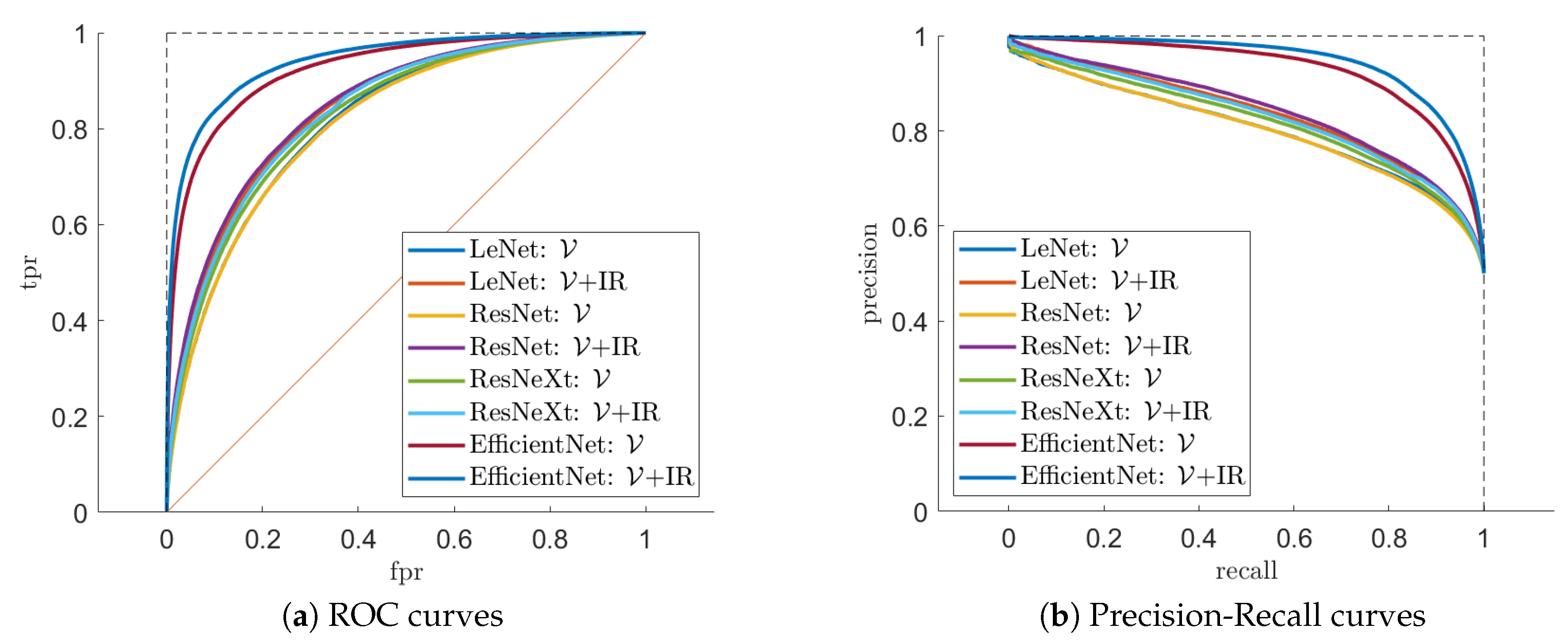
3.2. Classification Performance

The performance for the CNNs of interest was assessed employing the test dataset, which is composed of 426,792 records (see Figure 4 and Supplementary Materials). The experiments included using the $\mathcal{V}$ bands and the $\mathcal{V}$ + IR bands available. The Receiving Operating Characteristics (ROC) curve illustrates the trade-off between the sensitivity or true positive rate (TPR = TP/(TP+ FN)) and the complement to the specificity or false positive rate (FPR = FP/(FP+ TN)), where TP, FN, FP, and TN correspond to the number of true positives, false negatives, false positives, and true negatives, respectively. Correspondingly, the Precision-Recall shows the trade-off between the precision (P = TP/(TP+ FP) and the recall (R = TP/(TP+ FN)). Note that TPR and R are the same. Usually, practitioners use them separately when finding an optimal compromise between TPR and FPR or between P and R, which occurs at a specific decision threshold value ${\tau }_p$. The area under the curve (AUC), for the ROC and Precision-Recall, is a useful metric to evaluate the performance of a classifier. High TPR and low FPR values, over a wide range of thresholds, result in a large ROC AUC, while high values of both P and R generate a large Precision-Recall AUC.

Figure 5 shows the curves of TPR vs. FPR (ROC curve), precision vs. recall, for all the CNN architectures and the employment of the $\mathcal{V}$ bands and the $\mathcal{V}$ + IR bands.

Table 1. Performance for the CNNs under consideration is expressed as area under the curve (AUC) for ROC and Precision-Recall. The first two columns correspond to the analysis of $\mathcal{V}$ bands images, while the second two columns correspond to $\mathcal{V}$ + IR band images. We obtain the best performance with EfficientNet with $\mathcal{V}$ + IR bands. For these results (best in bold), the test dataset is employed.

	$\mathcal{V}$ Bands		$\mathcal{V}$ + IR Bands
CNN	ROC	Precision-Recall	ROC	Precision-Recall
LeNet-5	0.8164	0.8032	0.8422	0.8351
ResNet	0.8138	0.8022	0.8475	0.8417
ResNeXt	0.8284	0.8189	0.8376	0.8293
EfficientNet	0.9256	0.9286	0.9421	0.9457

shows the numerical values corresponding to the AUC for each case. Note that the use of the $\mathcal{V}$ + IR consistently outperforms the employment of the $\mathcal{V}$ bands for all the CNN architectures under consideration. Similarly, the EfficientNet architecture, with ROC AUC = 0.9421 and Precision-Recall AUC = 0.9457, outperforms the rest of the CNNs by a considerable margin.

4. Discussion

Vulnerability is a fluid concept that may include social, physical, health, educational, environmental, economic, and physicological aspects [48]. Nonetheless, its concrete definition is of paramount importance because its establishment will entail the subsequent approach to risk assessment and reduction efforts. Our approach to the definition of vulnerability aims to find a tradeoff between the terms proposed by UN-Habitat [27], the data publicly available for its countrywide detection [30], and an agnostic approach about the relative importance of the factors employed. Other sources of information, e.g., whether houses receive electricity, or prior knowledge of the importance of the different reference values may provide to be useful in a more refined labeling associated with the images and further performance of the automatic inference mechanisms, as shown by Sharma et al. [24] and Ibrahim et al. [23]. Establishing a baseline of comparison with other classical [8,12,16,22] or modern approaches [13,14,21,23,24] is most challenging. For one, the data sources, dense [8] or sparse [13], may have local and unique components; the scope may be a citywide [18], countrywide [26], or regionwide [15,25] interest. At any rate, this research demonstrates a strong performance with publicly available satellite information and census data at the fine-grained resolution of residential block and countrywide scale. There are some applications where the use of a CNN requires a control and experimental group [49,50,51]. That is the case for applications where the CNN is employed as an alternative procedure. In these circumstances, the control group is the golden standard to assess the effectiveness of a new technique. In the present research, there is no comparison with a previous method to determine vulnerability from satellite images because this study introduces both a source of information and a vulnerability index definition. However, in parallel to presenting a robust baseline by comparing different CNN architectures, this paper provides the means and forms to benchmark new approaches on the same framework.

This study is based on the reformulation of the census reference values as a classification problem where the distinction between vulnerable and non-vulnerable is the result of the lack of at least one UN-habitat reference value. These results extend Dorji et al. [16], who also framed their regression problem as a classification one employing nighttime-light satellite images and classical machine learning techniques, such as gradient boosting. These results show that this reformulation strategy can be applied also in the case of daytime-light satellite multispectral images and deep learning based models. In fact, this research distinguish from others using high resolution imagery [11,12,14], potentially making it more affordable.

The image resolution employed in this study is relatively coarse, although not uncommon in this field of study [8,17,19]. This choice may permit a widespread adoption of the method by allowing its application with to open datasets, contrary to the employment of private high-resolution satellite images such as QuickBird and DigitalGlobe images. Furthermore, there has been a sizable historical interest in the computer vision research community to understand the tolerance of detection algorithms to degradation in image resolution [52]. Despite that, the level of performance achieved in establishing the map between multispectral satellite images and census data is remarkable. Further research may explore how the deep learning algorithm may provide explanations for its decisions [53]. This line of study will open rich avenues for investigation, but most importantly, it will produce less bias and more ethical application of research results [54].

The availability of large-scale, long-term, satellite image datasets makes it possible to employ eager data methods, such as CNNs, which increase their performance logarithmically based on the volume of training data size [55]. Yet, models still play a role. For example, the comparison of diverse CNN architectures, varying in deep and complexity, highlights that while convolutions are important for feature extraction, one may find substantial differences in performance relative to their overall architecture, which may include the factors of width, depth, resolution, and cardinality employed by EfficientNet [38]. This result is still the subject of widespread interest in the deep learning community, as it remains debatable in which circumstances deeper networks are better than shallower ones [56].

An intriguing outcome in the results is the increase in performance achieved with the employment of the infrared bands. Recent studies on trees’ urban ecosystem services [57] point out the relationship between socioeconomic indicators and trees canopy. Further studies may shed light on whether the infrared bands capture some of the associated temperature differences commonly found across vulnerable communities [58].

5. Conclusions

This paper introduces an approach to detect vulnerability at the residential block level. It consists of training CNNs to find a relationship between salient features extracted from satellite images and vulnerability indicators obtained from population census data. Our extensive experimental results, including hundreds of thousands of records, with state-of-the-art CNN architectures, show that it is possible to create a high-performance characterization of this relationship, offering ample opportunity for generalization. In particular, our experiments show that EfficientNet CNN architectures provide the best performance relative to other topologies.

In the efforts to reduce vulnerability is important to provide decision-makers with affordable, reliable, and up-to-date information about its sprawl. Our method introduces a tool to rapidly assess the spatial distribution of poverty in Mexico in detail and with ample coverage. This methodology should be a helpful asset to decide expenditure and to evaluate the progress of remedy programs. Thus, focused attention to vulnerable communities should result in a more significant return on public and humanitarian funds.

In the future, the employment of satellite radar images will be explored. Although multispectral images from Landsat, in the visible and infrared bands, are readily available every 16 days, clouds or time of the day may alter their suitability. On the contrary, Sentinel-1 provides Synthetic Aperture Radar (SAR) images, which have a higher resolution, are unaffected by clouds and can be taken at any time of day, since they are from active sensors. Furthermore, although these results offer good average performance at a national level, it may be interesting to explore the opportunities left at a coarser level of analysis at regional, state, and municipalwide levels. Furthermore, these results make it possible to periodically evaluate vulnerable communities, even during years when censuses are not carried out by employing a blend of satellite imagery and deep learning techniques.

References

1. Atamanov, A.; Lakner, C.; Mahler, D.G.; Tetteh Baah, S.K.; Yang, J. The Effect of New PPP Estimates on Global Poverty; Technical Report; World Bank: Washington, DC, USA, 2020. [Google Scholar]
2. Akova, F. Effective Altruism and Extreme Poverty; Technical Report; University of Warwick: Coventry, UK, 2021. [Google Scholar]
3. Solt, F. Measuring Income Inequality Across Countries and Over Time: The Standardized World Income Inequality Database. Soc. Sci. Q. 2020, 101, 1183–1199. [Google Scholar] [CrossRef]
4. Scheuer, F.; Slemrod, J. Taxation and the Superrich. Annu. Rev. Econ. 2020, 12, 189–211. [Google Scholar] [CrossRef]
5. Roser, M.; Ortiz-Ospina, E.; Global Extreme Poverty. In Our World in Data. 2013. Available online: https://ourworldindata.org/extreme-poverty (accessed on 8 August 2021).
6. Plag, H.; Jules-Plag, S. A Goal-based Approach to the Identification of Essential Transformation Variables in Support of the Implementation of the 2030 Agenda for Sustainable Development. Int. J. Digit. Earth 2020, 13, 166–187. [Google Scholar] [CrossRef]
7. Khan, M.; Blumenstock, J. Multi-GCN: Graph Convolutional Networks for Multi-View Networks, with Applications to Global Poverty. In Proceedings of the AAAI Conference on Artificial Intelligence, Honolulu, HI, USA, 27 January–1 February 2019; Volume 33, pp. 606–613. [Google Scholar]
8. Bansal, C.; Jain, A.; Barwaria, P.; Choudhary, A.; Singh, A.; Gupta, A.; Seth, A. Temporal Prediction of Socio-economic Indicators Using Satellite Imagery. In COMAD; ACM: New York, NY, USA, 2020; pp. 73–81. [Google Scholar]
9. Hoffman-Hall, A.; Loboda, T.; Hall, J.; Carroll, M.; Chen, D. Mapping Remote Rural Settlements at 30 m Spatial Resolution using Geospatial Data-Fusion. Remote Sens. Environ. 2019, 233, 111386. [Google Scholar] [CrossRef]
10. Gram-Hansen, B.; Helber, P.; Varatharajan, I.; Azam, F.; Coca-Castro, A.; Kopackova, V.; Bilinski, P. Mapping informal settlements in developing countries using machine learning and low resolution multi-spectral data. In Proceedings of the AAAI/ACM Conference on AI, Ethics, and Society, Honolulu, HI, USA, 27–28 January 2019; pp. 361–368. [Google Scholar]
11. Verma, D.; Jana, A.; Ramamritham, K. Transfer Learning Approach to Map Urban Slums using High and Medium Resolution Satellite Imagery. Habitat Int. 2019, 88, 101981. [Google Scholar] [CrossRef]
12. Engstrom, R.; Hersh, J.; Newhouse, D. Poverty from Space: Using High-Resolution Satellite Imagery for Estimating Economic Well-Being; World Bank: Washington, DC, USA, 2017. [Google Scholar]
13. Herfort, B.; Li, H.; Fendrich, S.; Lautenbach, S.; Zipf, A. Mapping Human Settlements with Higher Accuracy and Less Volunteer Efforts by Combining Crowdsourcing and Deep Learning. Remote Sens. 2019, 11, 1799. [Google Scholar] [CrossRef] [Green Version]
14. Ajami, A.; Kuffer, M.; Persello, C.; Pfeffer, K. Identifying a Slums’ Degree of Deprivation from VHR Images using Convolutional Neural Networks. Remote Sens. 2019, 11, 1282. [Google Scholar] [CrossRef] [Green Version]
15. Andreano, M.S.; Benedetti, R.; Piersimoni, F.; Savio, G. Mapping Poverty of Latin American and Caribbean Countries from Heaven Through Night-Light Satellite Images. Soc. Indic. Res. 2020, 156, 533–562. [Google Scholar] [CrossRef]
16. Dorji, U.J.; Plangprasopchok, A.; Surasvadi, N.; Siripanpornchana, C. A Machine Learning Approach to Estimate Median Income Levels of Sub-Districts in Thailand using Satellite and Geospatial Data. In Proceedings of the ACM SIGSPATIAL International Workshop on AI for Geographic Knowledge Discovery, Chicago, IL, USA, 5 November 2019; pp. 11–14. [Google Scholar]
17. Shi, K.; Chang, Z.; Chen, Z.; Wu, J.; Yu, B. Identifying and Evaluating Poverty using Multisource Remote Sensing and Point of Interest (POI) Data: A Case Study of Chongqing, China. J. Clean. Prod. 2020, 255, 120245. [Google Scholar] [CrossRef]
18. Li, G.; Chang, L.; Liu, X.; Su, S.; Cai, Z.; Huang, X.; Li, B. Monitoring the spatiotemporal dynamics of poor counties in China: Implications for global sustainable development goals. J. Clean. Prod. 2019, 227, 392–404. [Google Scholar] [CrossRef]
19. Xie, M.; Jean, N.; Burke, M.; Lobell, D.; Ermon, S. Transfer Learning from Deep Features for Remote Sensing and Poverty Mapping. In Proceedings of the AAAI Conference on Artificial Intelligence, Phoenix, AZ, USA, 12–17 February 2016. [Google Scholar]
20. Ngestrini, R. Predicting Poverty of a Region from Satellite Imagery using CNNs; Technical Report; Utrecht University: Utrecht, The Netherlands, 2019. [Google Scholar]
21. Xie, S.; Girshick, R.; Dollár, P.; Tu, Z.; He, K. Aggregated Residual Transformations for Deep Neural Networks. In Proceedings of the IEEE Conference on Computer Vision and Pattern Recognition, Honolulu, HI, USA, 21–26 July 2017; pp. 1492–1500. [Google Scholar]
22. Roy, D.; Bernal, D.; Lees, M. An Exploratory Factor Analysis Model for Slum Severity Index in Mexico City. Urban Stud. 2019, 789–805. [Google Scholar] [CrossRef] [Green Version]
23. Ibrahim, M.; Haworth, J.; Cheng, T. Understanding Cities with Machine Eyes: A Review of Deep Computer Vision in Urban Analytics. Cities 2020, 96, 102481. [Google Scholar] [CrossRef]
24. Sharma, P.; Manandhar, A.; Thomson, P.; Katuva, J.; Hope, R.; Clifton, D.A. Combining Multi-Modal Statistics for Welfare Prediction Using Deep Learning. Sustainability 2019, 11, 6312. [Google Scholar] [CrossRef] [Green Version]
25. Jean, N.; Burke, M.; Xie, M.; Davis, M.; Lobell, D.; Ermon, S. Combining Satellite Imagery and Machine Learning to Predict Poverty. Science 2016, 353, 790–794. [Google Scholar] [CrossRef] [Green Version]
26. Tingzon, I.; Orden, A.; Sy, S.; Sekara, V.; Weber, I.; Fatehkia, M.; Herranz, M.G.; Kim, D. Mapping Poverty in the Philippines Using Machine Learning, Satellite Imagery, and Crowd-sourced Geospatial Information. Int. Arch. Photogramm. Remote Sens. Spat. Inf. Sci. 2019, XLII-4/W19, 425–431. [Google Scholar] [CrossRef] [Green Version]
27. United Nations Human Settlements Programme Staff. The Challenge of Slums: Global Report on Human Settlements, 2003; Earthscan Publications: London, UK; Sterling, VA, USA, 2003; ISBN 978-1-84407-037-4. [Google Scholar]
28. Weeks, J.; Hill, A.; Stow, D.; Getis, A.; Fugate, D. Can We Spot a Neighborhood from the Air? Defining Neighborhood Structure in Accra, Ghana. Remote Sens. 2007, 69, 9–22. [Google Scholar] [CrossRef] [PubMed] [Green Version]
29. Patel, A.; Shah, P.; Beauregard, B. Measuring Multiple Housing Deprivations in Urban India using Slum Severity Index. Habitat Int. 2020, 101, 102190. [Google Scholar] [CrossRef]
30. INEGI. Censos y Conteos de Población y Vivienda; INEGI: Aguascalientes, Mexico, 2011. [Google Scholar]
31. INEGI. Producción y Publicación de la Geomediana Nacional a Partir de Imágenes del Cubo de Datos Geoespaciales de México. Documento Metodológico; Technical Report; INEGI: Aguascalientes, Mexico, 2020. [Google Scholar]
32. Roberts, D.; Mueller, N.; McIntyre, A. High-dimensional pixel composites from earth observation time series. IEEE Trans. Geosci. Remote Sens. 2017, 55, 6254–6264. [Google Scholar] [CrossRef]
33. LeCun, Y.; Bengio, Y.; Hinton, G. Deep Learning. Nature 2015, 521, 436–444. [Google Scholar] [CrossRef]
34. Li, H.; Tian, Y.; Mueller, K.; Chen, X. Beyond Saliency: Understanding Convolutional Neural Networks from Saliency Prediction on Layer-wise Relevance Propagation. Image Vis. Comput. 2019, 83, 70–86. [Google Scholar] [CrossRef] [Green Version]
35. Deng, J.; Dong, W.; Socher, R.; Li, L.J.; Li, K.; Fei-Fei, L. Imagenet: A Large-Scale Hierarchical Image Database. In Proceedings of the IEEE Conference on Computer Vision and Pattern Recognition, Miami, FL, USA, 20–25 June 2009; pp. 248–255. [Google Scholar]
36. Abadi, M.; Agarwal, A.; Barham, P.; Brevdo, E.; Chen, Z.; Citro, C.; Corrado, G.S.; Davis, A.; Dean, J.; Devin, M.; et al. TensorFlow: Large-Scale Machine Learning on Heterogeneous Systems. Software. 2015. Available online: tensorflow.org (accessed on 8 August 2021).
37. He, K.; Zhang, X.; Ren, S.; Sun, J. Deep Residual Learning for Image Recognition. In Proceedings of the IEEE Conference on Computer Vision and Pattern Recognition, Las Vegas, NV, USA, 27–30 June 2016; pp. 770–778. [Google Scholar]
38. Tan, M.; Le, Q. Efficientnet: Rethinking Model Scaling for Convolutional Neural Networks. In Proceedings of the International Conference on Machine Learning, Long Beach, CA, USA, 9–15 June 2019; pp. 6105–6114. [Google Scholar]
39. LeCun, Y.; Boser, B.; Denker, J.; Henderson, D.; Howard, R.; Hubbard, W.; Jackel, L. Backpropagation Applied to Handwritten Zip Code Recognition. Neural Comput. 1989, 1, 541–551. [Google Scholar] [CrossRef]
40. Szegedy, C.; Vanhoucke, V.; Ioffe, S.; Shlens, J.; Wojna, Z. Rethinking the Inception Architecture for Computer Vision. In Proceedings of the IEEE Conference on Computer Vision and Pattern Recognition, Las Vegas, NV, USA, 27–30 June 2016; pp. 2818–2826. [Google Scholar]
41. Goodfellow, I.; Pouget-Abadie, J.; Mirza, M.; Xu, B.; Warde-Farley, D.; Ozair, S.; Courville, A.; Bengio, Y. Generative Adversarial Nets. arXiv 2014, arXiv:1406.2661. [Google Scholar]
42. Perez, A.; Ganguli, S.; Ermon, S.; Azzari, G.; Burke, M.; Lobell, D. Semi-Supervised Multitask Learning on Multispectral Satellite Images using Wasserstein Generative Adversarial Networks (GANs) for Predicting Poverty. arXiv 2019, arXiv:1902.11110. [Google Scholar]
43. Szegedy, C.; Ioffe, S.; Vanhoucke, V.; Alemi, A. Inception-v4, Inception-Resnet and the Impact of Residual Connections on Learning. In Proceedings of the AAAI Conference on Artificial Intelligence, San Francisco, CA, USA, 4–9 February 2017; Volume 31. [Google Scholar]
44. Sandler, M.; Howard, A.; Zhu, M.; Zhmoginov, A.; Chen, L.C. MobileNet v2: Inverted Residuals and Linear Bottlenecks. In Proceedings of the IEEE Conference on Computer Vision and Pattern Recognition, Salt Lake City, UT, USA, 18–23 June 2018; pp. 4510–4520. [Google Scholar]
45. Hu, J.; Shen, L.; Sun, G. Squeeze-and-Excitation Networks. In Proceedings of the IEEE Conference on Computer Vision and Pattern Recognition, Salt Lake City, UT, USA, 18–23 June 2018; pp. 7132–7141. [Google Scholar]
46. Buslaev, A.; Iglovikov, V.; Khvedchenya, E.; Parinov, A.; Druzhinin, M.; Kalinin, A. Albumentations: Fast and Flexible Image Augmentations. Information 2020, 11, 125. [Google Scholar] [CrossRef] [Green Version]
47. Glorot, X.; Bengio, Y. Understanding the Difficulty of Training Deep Feedforward Neural Networks. In Proceedings of the International Conference on Artificial Intelligence and Statistics, Sardinia, Italy, 13–15 May 2010; pp. 249–256. [Google Scholar]
48. Limongi, G.; Galderisi, A. Twenty Years of European and International Research on Vulnerability: A Multi-Faceted Concept for Better Dealing with Evolving Risk Landscapes. Int. J. Disaster Risk Reduct. 2021, 63, 102451. [Google Scholar] [CrossRef]
49. Wang, P.; Liu, X.; Berzin, T.; Brown, J.; Liu, P.; Zhou, C.; Lei, L.; Li, L.; Guo, Z.; Lei, S. Effect of a Deep-Learning Computer-Aided Detection System on Adenoma Detection during Colonoscopy (CADe-DB Trial): A Double-Blind Randomised Study. Lancet Gastroenterol. Hepatol. 2020, 5, 343–351. [Google Scholar] [CrossRef]
50. Dickson, I. A Trial of Deep-Learning Detection in Colonoscopy. Nat. Rev. Gastroenterol. Hepatol. 2020, 17, 194. [Google Scholar] [CrossRef] [PubMed] [Green Version]
51. Han, L.; Chen, Y.; Cheng, W.; Bai, H.; Wang, J.; Yu, M. Deep Learning-Based CT Image Characteristics and Postoperative Anal Function Restoration for Patients with Complex Anal Fistula. J. Healthc. Eng. 2021, 2021. [Google Scholar] [CrossRef]
52. Torralba, A.; Fergus, R.; Freeman, W. 80 Million Tiny Images: A Large Data Set for Nonparametric Object and Scene Recognition. IEEE Trans. Pattern Anal. Mach. Intell. 2008, 30, 1958–1970. [Google Scholar] [CrossRef]
53. Xie, N.; Ras, G.; van Gerven, M.; Doran, D. Explainable Deep Learning: A Field Guide for the Uninitiated. arXiv 2020, arXiv:2004.14545. [Google Scholar]
54. Birhane, A.; Prabhu, V. Large Image Datasets: A Pyrrhic Win for Computer Vision? In Proceedings of the IEEE Winter Conference on Applications of Computer Vision, Waikoloa, HI, USA, 3–8 January2021; pp. 1536–1546. [Google Scholar]
55. Sun, C.; Shrivastava, A.; Singh, S.; Gupta, A. Revisiting Unreasonable Effectiveness of Data in Deep Learning Era. In Proceedings of the IEEE International Conference on Computer Vision, Venice, Italy, 22–29 October 2017; pp. 843–852. [Google Scholar]
56. Malach, E.; Shalev-Shwartz, S. Is Deeper Better only when Shallow is Good? arXiv 2019, arXiv:1903.03488. [Google Scholar]
57. Alves Carvalho Nascimento, L.; Shandas, V. Integrating Diverse Perspectives for Managing Neighborhood Trees and Urban Ecosystem Services in Portland, OR (US). Land 2021, 10, 48. [Google Scholar] [CrossRef]
58. Saverino, K.; Routman, E.; Lookingbill, T.; Eanes, A.; Hoffman, J.; Bao, R. Thermal Inequity in Richmond, VA: The Effect of an Unjust Evolution of the Urban Landscape on Urban Heat Islands. Sustainability 2021, 13, 1511. [Google Scholar] [CrossRef]
Figure 1. Detecting vulnerable communities via satellite imagery and population census. Our approach collects multispectral satellite images corresponding to the census information of residential blocks in Mexico. After training and assessing the performance of diverse convolutional neural networks, the results demonstrate that it is possible to establish a robust mapping between satellite images and vulnerability. This outcome should permit an accurate and up-to-date establishment of the spatial socioeconomic distribution of vulnerable communities in the country.
Remotesensing 13 03603 g001
Figure 2. Reference values and vulnerability index histograms. The reference values correspond to population responses to the census questions. The responses are averaged for the houses in each of the 2,178,508 residential blocks in Mexico. Note that 60.23%, 6.75%, 59.81%, 11.18%, and 60.49% have (corresponding to a value of zero in the histogram) and 0.43%, 12.16%, 0.88%, 0.45%, 0.13% do not have (corresponding to a value of one in the histogram) sewage, toilets, running water, an occupancy of more than three people per bedroom, and concrete floors, respectively. In the case of occupancy, for 99.54% of the records, the average occupancy is larger than three for 9834 of the records. The vulnerability index v is defined in (1).
Remotesensing 13 03603 g002
Figure 3. Sample of Landsat-7 satellite images corresponding to the visible ( V ) bands centered in residential blocks across Mexico. Each image (ao) corresponds to a 600 × 600 m geographical region.
Remotesensing 13 03603 g003
Figure 4. Mapping vulnerability in Mexico using satellite images. (a) shows the location of the 2,178,508 residential blocks delimited by INEGI [30]. (b) illustrates the vulnerability assessment for Mexico. (cg) and (hl) show the assessment of vulnerability for Mexico City and the city of Acapulco in the Mexican state of Guerrero. Besides showing the results at different spatial scales, this illustration provides a comparison between Ground Truth (non-vulnerable in yellow and vulnerable in red) and the different CNN architectures (with a color palette from yellow to red).
Remotesensing 13 03603 g004
Figure 5. Performance of the different CNN architectures with different arrangement of bands.
Remotesensing 13 03603 g005