
Monitoring of Water Level Change in a Dam from High-Resolution SAR Data


1
Department of Energy Resources and Geosystems Engineering, Sejong University, Seoul 05006, Korea
2
Department of Geological Sciences, Pusan National University, Busan 46241, Korea
*
Author to whom correspondence should be addressed.
Remote Sens. 2021, 13(18), 3641; https://0-doi-org.brum.beds.ac.uk/10.3390/rs13183641
Submission received: 25 July 2021
/
Revised: 25 August 2021
/
Accepted: 9 September 2021
/
Published: 12 September 2021
(This article belongs to the Special Issue Advances in Spaceborne SAR – Technology and Applications)
Abstract
:Accurate measurement of water levels and variations in lakes and reservoirs is crucial for water management. The retrieval of the accurate variations in water levels in lakes and reservoirs with small widths from high-resolution synthetic aperture radar (SAR) images such as the TerraSAR add-on for Digital Elevation Measurements (TanDEM-X) and COnstellation of small Satellites for the Mediterranean basin Observation (COSMO-SkyMed) are presented here. A detailed digital surface model (DSM) for the upstream face of the dam was constructed using SAR interferometry with TanDEM-X data to estimate the water level. The elevation of the waterline below that of the interferometric SAR (InSAR) DSM was estimated based on upstream face modeling. The waterline boundary detected using the SAR Edge Detection Hough Transform algorithm was applied to the restored DSM. The SAR-derived water level variations showed a high correlation coefficient of 0.99 and a gradient of 1.08 with the gauged data. The difference between the gauged data and SAR-derived data was within ±1 m, and the standard deviation of the residual was 0.60 m. These results suggest that water level estimation can be used as an operational supplement for traditional gauged data at remote sites.
1. Introduction
Dams and impoundments have been built to enable the storage of water necessary during the dry season and to control flooding, recreation, navigation, and the generation of hydropower [1,2]. Water level monitoring is essential because lakes and reservoirs are proxies for understanding global climate change [3]. Once the water volume has been determined and combined with precipitation, evaporation, and inflow, the water balance of lakes and reservoirs can be used to estimate the outflow [4]. However, the large uncertainties associated with projected precipitation changes make it difficult for the responsible agencies to perform water management practices, such as water allocation and water release strategies. Therefore, accurate measurement of water levels and monitoring of variations in lakes and reservoirs are essential for equitable water allocation to water management and ecosystem services and to improve the understanding of the impacts of climate change [5,6].
Acquiring water-level information is impossible if in situ gauge data are inadequate, if the regions are politically inaccessible, or if lakes and reservoirs are in remote areas [7]. To overcome these limitations, remote sensing data have been used to measure water levels and estimate water storage. Satellite altimetry products have been combined with surface water areas (or surface water extent) derived from optical sensors, such as the Moderate Resolution Imaging Spectroradiometer (MODIS), Landsat TM/ETM+, and synthetic aperture radar (SAR) imagery (e.g., RADARSAT, JERS-1 and ERS-1/2) [5,8,9]. Most of these studies have relied on the accuracy of the retrieved water levels, which strongly depend on the size of the lake or reservoir and the accuracy of water land boundaries defined by delineation methods [10,11]. The characteristics of radar altimetry restrict its application to many lakes and reservoirs that are smaller than approximately 2 km wide, because of their large footprint size (several kilometers) and limitations due to orbital and atmospheric errors [12,13].
In optical imagery, the surface water area is delineated by a threshold of vegetation or a water index. Although the surface water area is suitable for optical imagery such as Landsat, SPOT, and MODIS, the spatial resolution of MODIS is too low for small lakes, and it is strongly limited by weather conditions such as clouds and smoke [8,14,15]. Recently, the monthly dynamics of water extent were estimated for both national and local scales (two lakes) using Sentinel-2 with 10 m spatial resolution [16]. SAR-based estimation of the surface water area is limited by the roughening of surface water by the wind [16]. Interferometric phases with high coherence were used to delineate the inundated surface area based on the scattering characteristics of vegetated areas above surface water [17,18,19].
Although synthetic aperture radar interferometry (InSAR) observations have been used successfully to study wetland hydrology [20,21], this method is suitable for a wide area with a gentle slope where the exposed area depends on the water level. Therefore, whether or not reliable estimates of water levels in lakes and reservoirs with small widths can be obtained from satellite data remains unknown. A study to estimate the precise water level in a dam reservoir using accurate boundary extraction and a fine InSAR-based digital elevation model (DEM) was successfully introduced [22]. Although the technical feasibility of water level estimation from high-resolution SAR images was presented, further research is necessary to analyze the water level measurement performance using this method.
The main objective of this study is to provide a fully automated approach for waterline detection and water level estimation based on two cases: (1) when the digital surface model (DSM) of the upstream face is available, and (2) when only the slope angle of the bank is known. With time-series SAR data including large variations in water level, water level dynamics in a dam and reservoir with a steep slope are compared with in situ data. The performance of the proposed water level measurement method was determined by analysis of COSMO-SkyMed and TanDEM-X SAR data.
2. Study Area and Materials
2.1. Study Area
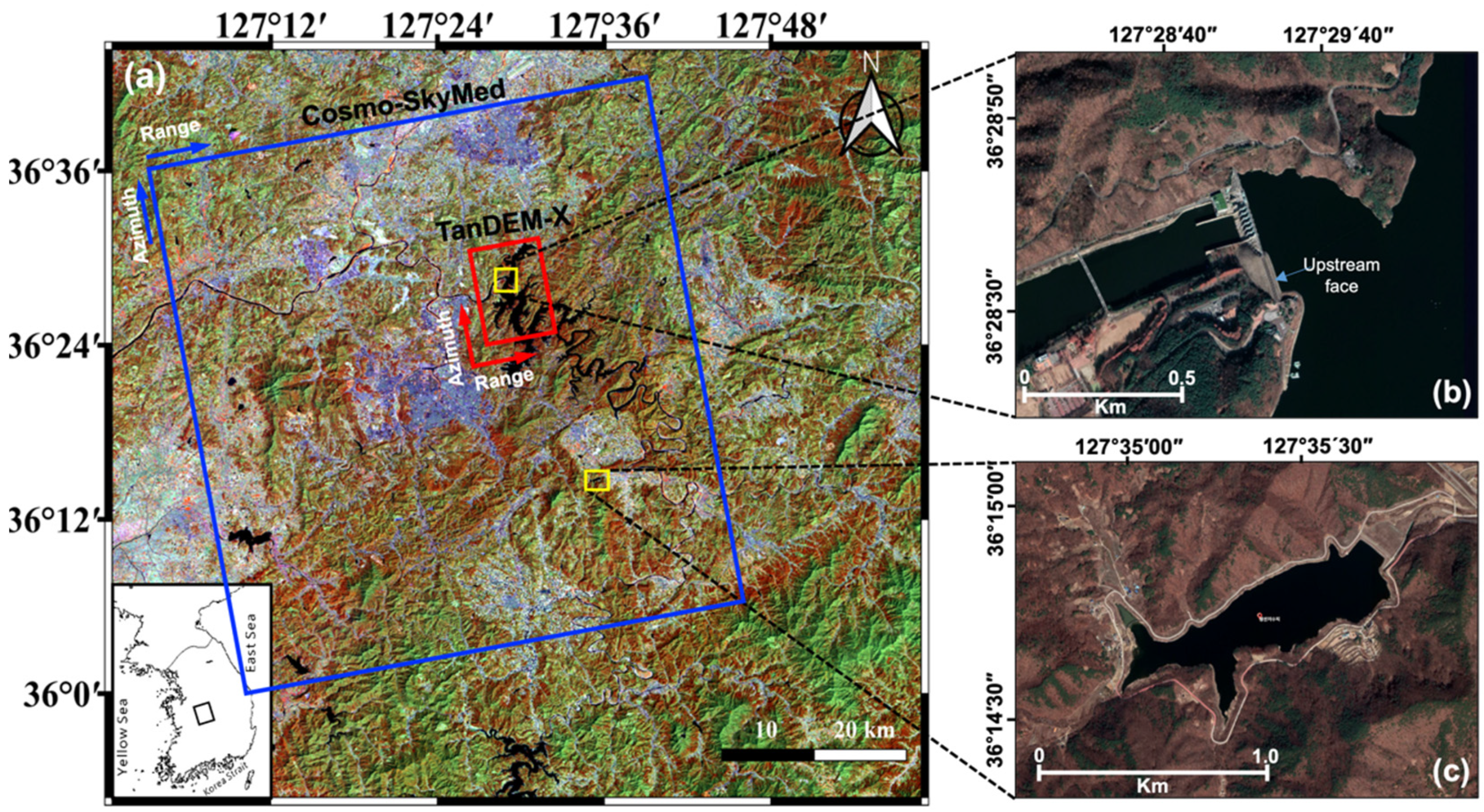
The Daecheong Dam, located at 36°28.59′N, 127°28.94′E (Figure 1b), is a multipurpose dam that provides flood control, a water supply source, and hydroelectric power generation. The dam is a type of embankment and is 7.2 × 49.5 m2. Construction started in 1975 and was completed in 1980 [23]. The Daecheong Reservoir has a 72 km2 surface area, was created during the dam’s construction, is upstream of the Geum River, and is a branch-type, dimictic, and temperate lake with a storage capacity of 1.49 billion m3 [24]. The Jangchan Reservoir, located at 36°14.74′N, 127°35.40′E (Figure 1c), is an agricultural reservoir upstream of Iwoncheon constructed in 1979. Its watershed area is 35.4 km2, and its effective storage capacity is 3.92 × 10⁶ m3 [25]. We selected these two sites as test sites because their gauge data are available. In addition, both sites are substantially affected by the annual rainfall cycle, and the annual water level change is approximately 10 m.
2.2. Data
2.2.1. TanDEM-X
TanDEM-X (TerraSAR add-on for Digital Elevation Measurement; TDX) is an innovative satellite SAR interferometer based on two TerraSAR-X (TSX) radar satellites flying in close formation [26]. Since June 2010, TSX has an identically constructed twin satellite (TDX) operated by the German Aerospace Center (DLR). The primary objective of the TDX mission was to generate a global DEM with a spatial resolution of 12 m and a relative vertical accuracy of 2 m for flat terrain. The revisit period was 11 days. The basic acquisition mode for the TDX mission is a combination of stripmap imaging and bistatic interferometric modes [27]. With the contribution of TDX bistatic InSAR pairs, a highly accurate World DEM generation could be achieved by eliminating atmospheric decorrelation due to repeated pass data acquisition [28]. In this study, TanDEM-X images acquired on 13 April 2011 were used for digital surface model (DSM) generation around the Daecheong Dam and based on InSAR application.
2.2.2. COSMO-SkyMed
COSMO-SkyMed (COnstellation of small Satellites for Mediterranean basin Observation, or CSK) is the first Italian dual-use (civil and military) constellation of satellites for Earth observation. CSK operates in a sun-synchronous orbit at an altitude of approximately 619.6 km. CSK is composed of four low-Earth orbit mid-sized satellites that were launched between 2008 and 2010, each equipped with a multimode high-resolution SAR operating in the X-band. All the satellites were equipped in the same orbital plane. Each satellite has a 16-day orbit cycle. Acquisition modes with one polarization were selected for HH, VV, VH, or HV. In this study, 30 single-look complex (SLC) images from Level 1A product images acquired between February 2013 and January 2016 were used for water level analysis. All images were acquired on the same orbit track at an incidence angle of 32.27° and HH polarization in stripmap mode with a 1.142 m range spacing and 1.924 m azimuth spacing. A detailed description of the images used in this study is provided in Table 1.
2.2.3. Gauged Data
For the Daecheong Dam, in situ daily water levels at a gauging station were obtained from the K-water from 1997 to 2017 [29]. These in situ measurements were used to validate the water levels estimated in this study. For the Jangchan Reservoir, in situ daily water levels at a gauging station were obtained from the Rural Agricultural Water Resource Information System operated by the Korea Rural Community Corporation [30]. Both gauged data were recorded every 10 min.
3. Methods
The water level measurement method introduced by Yoon et al. [22] was adopted to manage the CSK data. Depending on the possibility of DSM generation for the exposed upstream face of the dam or bank, the water level estimation method should differ. For dams or banks sufficiently large enough, a detailed DSM was generated using SAR interferometry with TanDEM-X data.
The water level estimation comprised two steps. First, the generated detailed DSM was used for the upstream face modeling (hereafter, slope modeling) to obtain the elevation (or level) of the waterline below that of the InSAR DSM. Second, an accurate waterline, the boundary between a water body and an exposed upstream face of a dam (Figure 2), was detected using the SAR edge detection Hough transform (SEDHT) algorithm [22]. Unfortunately, a detailed DSM for the upstream face of the dam or bank could not always be generated. Therefore, we also used a simple method to estimate the relative water level change, assuming a constant slope in the absence of a DSM for the particular dam slope.
3.1. Generation of an InSAR DSM for the Upstream Face of the Dam
A DSM of the dam structure can be built through a variety of methods, including leveling, photogrammetry, GPS, and InSAR. InSAR using TerraSAR-X was used to build a DSM over the dam, and the root mean square error between the TerraSAR-X InSAR DSM and the GPS-based DSM of the upstream face was 88 cm according to Yoon et al. [22]. TanDEM-X paved the way for detailed and accurate DEM generation by flying in a close orbit formation. The German Aerospace Center (DLR) announced the targeted relative and absolute vertical accuracy of the TDX World DSM as 2 m and 6 m, respectively [31]. However, no detailed analysis of the TanDEM-X DSM has been conducted in inclined areas or for various land covers [32]. The interferometric processing of TanDEM-X data was accomplished using in-house and GAMMA software [33]. InSAR DSM SAR processing was performed on TanDEM-X data using the co-registered single-look slant-range complex format provided by the DLR. The perpendicular baseline of the TanDEM-X data was 341.2 m, and the ambiguity height was −44.3 m. The flow of the DSM generation is shown in Figure 3. The interferogram was flattened using a 1-arc second (~30 m) Shuttle Radar Topography Mission (SRTM) DEM. The coherence image was derived from the interferogram filtered using a 7 × 7 adaptive spatial filter. The filtered image was subjected to phase unwrapping using a minimum cost flow algorithm. The unwrapped phase was added to the simulated phase from the SRTM and converted into height values using an interferometric geometry. The final geocoded InSAR DSM was produced using UTM coordinates.
A highly accurate InSAR DSM was generated. However, estimating the water level is not always possible if the waterline is extracted from an image located below the water level of the InSAR DSM. To solve this problem, Yoon et al. [22] proposed performing dam slope modeling of the InSAR DSM while assuming that the inclination of the upstream slope is constant. Slope modeling proceeded as the interferometric phase was filtered out at the water body according to the water level at the time the TDX data were taken, after which modeling processing was conducted through extrapolation. This step enables the boundary line to be extracted from the lower water level to overlay the restored InSAR DSM.
3.2. Waterline Boundary Detection
All SLC images were co-registered to a reference image using amplitude correlation to match the dataset to its radar coordinates. Because interferometric analysis is not relevant to this step procedure, any data can be selected as a reference. However, to reduce the co-registration error, an image in the middle of the data collection period and baseline (the distance between repeat orbits) can be a good candidate. In this study, the first CSK image acquired on 8 February 2013 was selected as the reference. An area of approximately 0.8 × 0.8 km² (400 × 400 pixels) centered on the Daecheong Dam was cropped from the 40 × 48 km² SLC images. All CSK SLC images were converted into intensity images.
In SAR images, the edge between land and water can be easily detected because the backscattering on the waterbody is low by specular reflection on water. However, when the water surface is roughened by wind, it is difficult to find the boundary because of the increased backscatter on the water surface. SEDHT can be applied without edge detection or spatial filtering to reduce speckle noise. The CSK stripmap mode data were noisy, making it difficult to discern the boundary between the water body and an exposed slope, especially in windy day images.
To reduce noise disturbance, Castan’s infinite symmetric exponential filter (ISEF) was applied to all the CSK intensity images. The ISEF uses a filter of infinite size to control the effects of noise as much as possible, with a sharp profile in its center to improve the precision of localization [34]. Therefore, it has better signal-to-noise ratios and better localization than other common noise suppression filters, such as the mean and median [35]. Even without spatial filtering, most of the data showed precise results, except for some data taken on a windy day. Comparing the results with no filter applied, the median filter showed better and worse results, while the ISEF always showed the best results from all data.
The SEDHT algorithm was applied to the ISEF-filtered images, which is a boundary detection algorithm based on the Hough transform. The result of the SEDHT image is expressed as H(, ), where is the distance from the origin to the closest point on the straight line, and is the angle between the x-axis and the line connecting the origin with the closest point. The differentiation is calculated as the difference between the H( + 1, ) and H( − 1, ) values on the right and left sides of H(, ) along the -axis in the Hough domain. The maximum differentiation value along the -axis in the Hough domain corresponds to the boundary line between the upstream face of the dam and the water body because an amplitude image was used instead of a binary image of the edge map generated by an edge detector. The boundary can be effectively detected while preserving SAR spatial resolution. The boundary detected by SEDHT imposed on the restored TDX InSAR DSM by the dam slope model was used to estimate the height of the detected line corresponding to the water level.
3.3. Relative Water Level Estimation
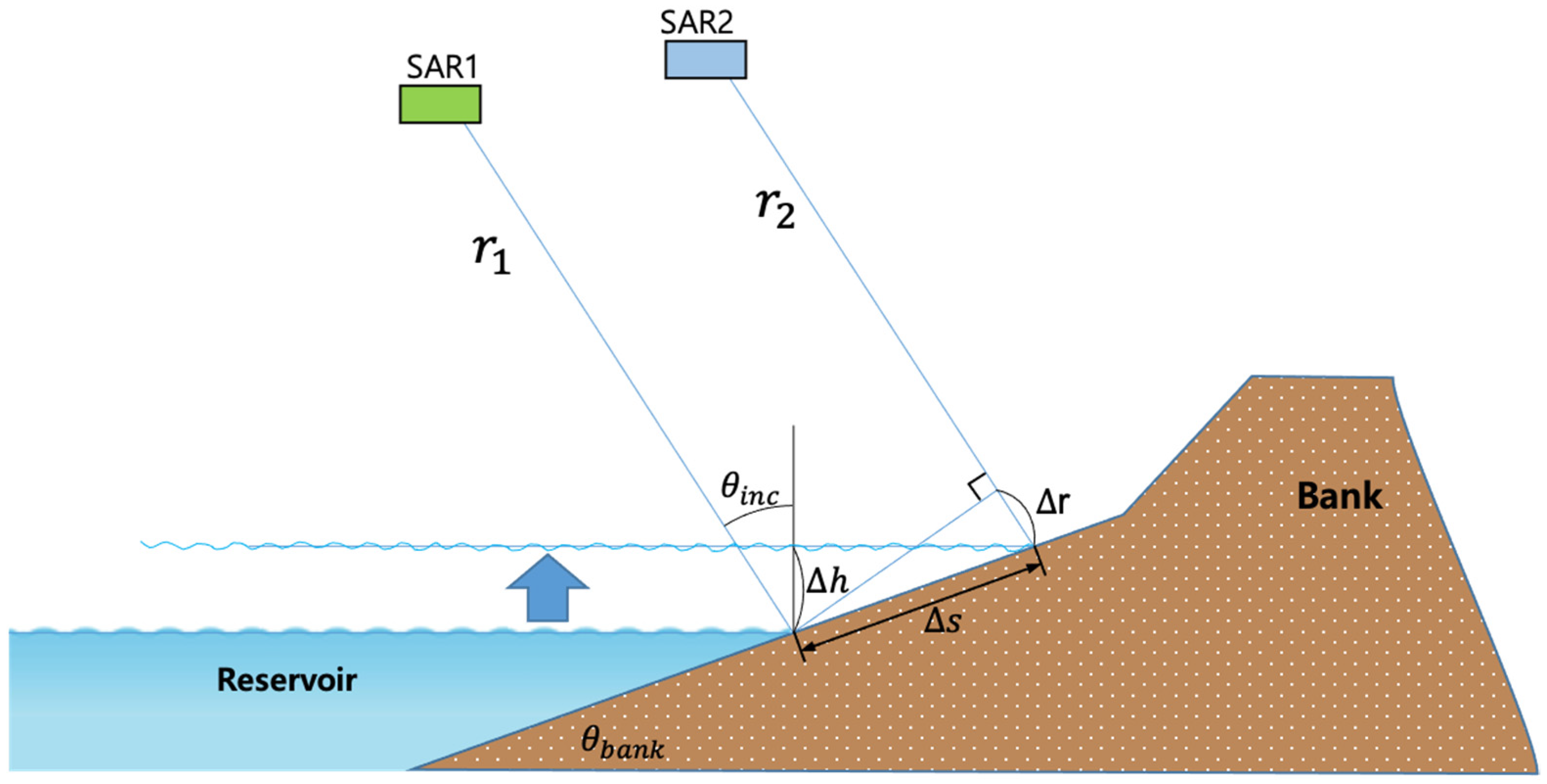
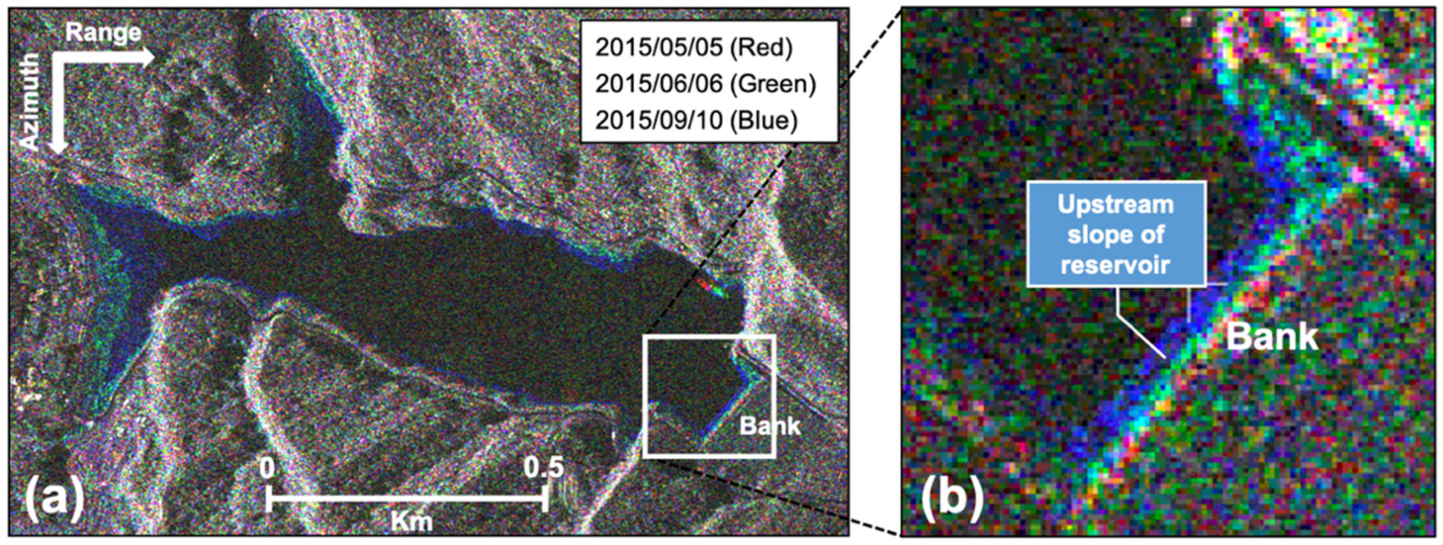
Figure 4 shows the pseudo RGB composite image produced with three CSK images from 5 May 2015, 6 June 2015 and 10 September 2015, with different water levels. Although changes in the water surface are more clearly observed on the left side of the gentle slope than on the bank on the right side, the DSM that includes the elevation at the bottom of the reservoir must be set in advance to extract the elevation at the gentle slope according to water level changes. However, the relative water level change can be estimated using the DSM or at least the slope of the bank. In particular, when creating a DSM of a bank structure is difficult, the relative water level change can be detected by assuming that the bank is a plane with a constant slope. In Figure 2, the distance in the range direction ( is different because of the backscattering change between the water surface and the exposed upstream face of the bank. The relationship between the relative water level change ( and the range distance change ( associated with the movement of the boundary line is as follows:
where is the distance along the upstream face due to water level change, and and are the SAR sensor’s incidence angle and the slope of the upstream face, respectively. As the slope of dams or banks is close to the incidence angle of the SAR sensor, the sensitivity to the slant range change ( according to the water level change () decreases, as shown in Equation (3). Information on the slope of the upstream face can be obtained from the auxiliary data on a reservoir. Alternatively, instead of creating a DSM of the upstream face, InSAR or photogrammetry can be applied to estimate the slope angle only, which may cover part of the upstream face.
4. Results
4.1. Measurement of Water Levels with DSM
The SAR data collected from the ascending and descending orbits showed different radar distortions on the dam slope. To investigate the actual conditions, we analyzed the InSAR DSMs generated using a descending orbit as well as an ascending orbit. The descending image shows foreshortening on the upstream face of the dam that may cause squeezing of the fringes on the dam surface, while the ascending image shows the slope of the upstream face well. Therefore, the TDX InSAR DSM generated from the ascending image acquired on 13 April 2011 was used for water level estimation.
Because of the short temporal baseline of only 0.14 s, highly coherent interferometric phases over 0.7 were well maintained at the dam structure and over nearly the entire scene, including forests and vegetation areas. Detailed topographic characteristics of the upstream face of the dam were retrieved using a 4 m × 4 m pixel spacing based on a 2 × 2 multi-looked interferogram. Figure 5a shows the final InSAR DSM generated using the ascending TDX data presented in Table 1. To enhance topographic details, the InSAR DSM was displayed with a fringe of 100 m height. The fringe is a complete color cycle (cyan, purple, magenta, yellow, and green). The accuracy of the generated DSM was not analyzed, as reference data were not available. The final geocoded InSAR DEM was generated using UTM coordinates. Since it also includes the geometry and structure of the dam slope, it will be referred to as DSM hereafter.
All CSK SLC images were acquired in ascending mode, similar to TanDEM-X, for the water level measurement on the upstream face of the Daecheong Dam. Because the boundary detection must be performed in range and azimuth radar coordinates to preserve the edge well, the geocoded TDX DSM must be transformed into a radar-coordinated DSM using the orbit of each SAR dataset. Figure 6a shows the height from the TDX InSAR DSM, overlaid with the amplitude CSK image acquired on 8 February 2013. The water gate of the dam appeared clearly in the middle of the image because of multiple scattering. The upstream face of the dam was located below the water gate. Based on the TDX InSAR DSM, which includes only a part of the slope, the extent of the DSM surface to the bottom of the upstream surface was modeled by fitting a planar equation (Figure 6b).
The SEDHT approach was applied for boundary extraction of all the CSK images. Figure 7 shows an example of SEDHT application to the ISEF-filtered amplitude image on 8 February 2013. Figure 7a shows the SEDHT image of the amplitude image in the Hough domain. Figure 7b shows the maximum differentiation value along the -axis in the Hough domain. In this example, a precise boundary line is detected at = −9 and = 85.5°.
All CSK SLC images were co-registered to a chosen reference image (8 February 2013) to match the radar coordinates. With these co-registered SLCs, we can use the same radar coordinated DSM for water level estimation, instead of making radar coordinated DSMs for each CSK image with a slightly different orbit trajectory. However, when the SAR data are acquired on different orbits or imaging geometries, the radar coordinated DSM should be generated for each SAR dataset. Figure 8 shows the results of the water-level measurement processing steps. In contrast to Yoon et al. [22], we applied the ISEF filter to reduce noise in the CSK amplitude image before the SEDHT algorithm was applied (Figure 8c). Although filtering occurs, blurring spatially by reducing noise, a 1 × 1 MLI CSK enabled precise extraction of the boundary line. The boundary detected by SEDHT was imposed on the restored TDX InSAR DSM using the dam slope model (Figure 8e,f). The mean water level was 95.5 m with a standard deviation of 0.32 m. The water levels for all CSK collections were observed by applying the method described above.
4.2. Comparison with In Situ Measurement
The water level change of the dam is strongly influenced by the annual rainfall cycle. Thus, we validated and detected the water level changes in dam reservoirs. First, the water boundaries were extracted by SEDHT and imposed on the restored TDX InSAR DSM, and the estimated water levels were compared with gauge data provided by the K-water. The gauge station was immediately adjacent to the target slope. The water level at the time of CSK image observation was obtained through interpolation of gauged data measured every 10 min. The water level recorded by the gauge station is the orthometric height. The elevation in the TDX InSAR DSM is the WGS84 ellipsoidal height. Before the comparison with the gauge station data, the mean geoid height (25 m) around the dam was used to compensate for the elevation difference (Figure 9a).
Even after compensating for the geoid height, there was still a slight difference in water levels between the gauged water levels (square dotted line in Figure 9a) and the SAR measurement (solid circle in Figure 9a). This difference may be due to the inaccuracy of the absolute phase calibration during the generation of the TDX DSM and/or the uncertainty of the reference height of the in situ gauge. Instead of compensating for the geoid height around the dam, the average water level difference (23.01 m) between the ellipsoidal height from the measured SAR and the orthometric height from the gauge station were subtracted. The trend of water level changes in the gauge data (open square dotted line in Figure 9a) and SAR-derived data (solid circle line in Figure 9a) were well matched. The difference between the gauged data and SAR-derived data (triangle dotted line) was within ±1 m, and the standard deviation of the residual was only 0.60 m.
Figure 9b shows a comparison of the SAR-measured water level before the geoid height compensation and the gauged water level at the station. A correlation coefficient of 0.99, and a gradient of 1.08, were obtained. Despite a shift, the high correlation coefficient and a gradient of approximately 1 indicated successful water level measurements in the dam using SAR with high accuracy.
4.3. Measurement and Comparison of Relative Water Levels without DSM
Unlike the Daecheong Dam, the bank in the Jangchan Reservoir does not have a sufficiently good interferometric phase to generate DSM using TanDEM-X images because the extent of the bank slope exposed above the water level is too small. Here, we used several CSK interferograms with a very short time interval and well-exposed upstream faces in both CSK SAR images. The selected CSK interferograms were stacked and averaged to obtain a slope model. Considering the quality of DSM and for testing Equation (3) to estimate the relative water level using only the slope of the bank (), we extracted a slope angle of 16° from the rough slope model. The SEDHT approach was applied to 30 CSK images. Relative water levels were calculated using Equation (3). The estimated relative water levels were compared with the absolute water levels measured at the Jangchan Reservoir station.
The trend of water level changes demonstrated by the gauge data (solid circle line in Figure 10a) and SAR-derived data (square dotted line in Figure 10a) was in good agreement. Figure 10b shows a scatter plot of the water levels observed at the gauging station and the relative water levels obtained by the proposed method. The slope of the first-order linear regression analysis was 1.08, and the squared correlation coefficient was 0.975. However, when the observed water level at the station was between 164 and 167 m, the relative water level by SAR remained at almost 0 m. In Equation (3), the range change according to the water level change is proportional to the difference between the incident angle of a satellite and the bank slope. Even if the slope of the bank and the sensor’s incidence angle are equal, there is no change in the slant range distance ( owing to the water level change. The field survey confirmed that the slope of the upper part of the bank slope was higher than that of the lower part. Therefore, we believe that the SAR measurements of 0 m are associated with the change in bank slope close to the incident angle of the satellite (32°).
5. Discussion
The measured water level correlated well with the gauge station data, but the accuracy of the measured water level according to this study was affected by the precision of the InSAR DSM. The TDX and CSK data used for the water level measurements in this study were acquired in stripmap mode with a spatial resolution of approximately 2 m. Although the spatial resolution of data in stripmap mode is worse than that in spotlight mode, the InSAR DSM generation using TDX data in stripmap mode showed good precision for providing water level estimation results. We posit that the TDX data on the spotlight mode improve the precision of InSAR DSM construction, and subsequently, water level measurements.
Unlike optical data, the intensity of the slope can vary according to the radar distortion, such as layover and foreshortening, according to the local incidence angle. The proposed method depends on the slope structure of the upstream face. Therefore, the targeted upstream face should be selected according to the geometric characteristics of the dam structure and the surrounding topography. SAR data should also be collected under favorable conditions to fit the targeted area, and the geometric characteristics of the dam structure and surrounding topography should be considered.
In addition, SAR data with different acquisition parameters (orbit, look direction, incidence angle, and resolution) can introduce additional errors in the water level estimation. For example, each image with a different incidence angle requires different DSMs with radar coordinates (range, azimuth) for each image. The coordinate transformation from a map coordinate to a radar coordinate can cause errors due to orbit inaccuracies. Therefore, SAR data collection using the same acquisition parameters, such as interferometric pairs, is preferred over multi-temporal data collected with various imaging geometries.
The main limitation of applying the proposed technique is that a long stretch of the upstream face is required. In addition, a DSM of slope, or at least a slope angle, is required. A DSM of the dam structure can be generated using InSAR, GPS survey [22], or other surveys such as photogrammetry. When the DSM generation of the area of interest is not applicable because of the lack of data or the limited extent of the upstream face, the slope angle from the auxiliary report for reservoirs can be used.
6. Conclusions
Knowledge of water level variations in reservoirs and dams is essential for water balance studies, water allocation, and water release strategies. The main objective of this study was to detect waterlines and estimate water level changes using only high-resolution SAR interferometry and amplitude images. The TDX InSAR DSM of the dam structure was generated from the ascending image, which was more favorable for water level estimation on the targeted slope acquired on 13 April 2011. The extent of the DSM surface to the lower part of the upstream face was modeled as a plane on the basis of the TDX InSAR DSM, covering only a part of the slope. The waterline detected by SEDHT was imposed on the restored TDX InSAR DSM using the dam slope model, and the water level was estimated. The difference between the gauged data and SAR-derived data was within ±1 m with 0.60 m of a standard deviation of residual, and comparison of the SAR-measured water level before the geoid height compensation against the gauged water level at the station had a correlation coefficient of 0.99. This result is meaningful because we estimated water level changes in a dam reservoir using only X-band SAR data without in situ gauge measurements.
In 2025, the Ministry of Environment and K-water plan to launch the next-generation medium satellite No. 5 (water resource/water disaster satellite) equipped with C-band SAR [36]. In future work, research on detecting waterlines on dams and estimating water level changes in dam reservoirs by using water resource/water disaster satellites will enable the monitoring of dams and reservoirs without in situ gauges in the Korean Peninsula, including North Korea, which is extremely limited due to geographical and political access.
Author Contributions
Y.-K.L., in situ data curation and writing of original draft preparation; S.-H.H., TanDEM-X data curation and contributed to the discussion of the results; S.-W.K., COSMO-SkyMed data curation, validation, and review of the results and organized the paper. All authors contributed to the writing of the article and the interpretation of the results and agreed on the conclusion. All authors have read and agreed to the published version of the manuscript.
Funding
This research was supported by the Space Core Technology Development Program through the National Research Foundation of Korea (NRF) grant funded by the Ministry of Science and ICT(NRF-2018M1A3A3A02066002). This research was also a part of the project titled ‘Development of smart maintenance monitoring techniques to prepare for disaster and deterioration of port infrastructure’ funded by the Ministry of Oceans and Fisheries, Korea.
Data Availability Statement
The gauged data can be found here: http://wamis.go.kr and https://rawris.ekr.or.kr. The SAR data sharing is not applicable to this article due to privacy.
Acknowledgments
We would like to thank the German Aerospace Center for access to the TanDEM-X data through the DLR projects (No. NTI_INSA0646).
Conflicts of Interest
The authors declare no conflict of interest.
References
- Cochrance, T.A.; Arias, M.E.; Piman, T. Historical impact of water infrastructure on water levels of the Mekong River and the Tonle Sap system. Hydrol. Earth Syst. Sci. 2014, 18, 4529–4541. [Google Scholar] [CrossRef] [Green Version]
- WCD. Dams and Development, a New Framework for Decision-Making, the Report of the World Commission on Dams; Earthscan Publication Ltd.: London, UK; Sterling, VA, USA, 2000; p. 404. [Google Scholar]
- Cretaux, J.F.; Abarca-del-Rio, R.; Berge-Nguyen, M.; Arsen, A.; Drolon, V.; Clos, G.; Maisongrande, P. Lake Volume Monitoring from Space. Surv. Geophys. 2016, 37, 269–305. [Google Scholar] [CrossRef] [Green Version]
- Duan, Z.; Bastiaanssen, W.G.M. Estimating water volume variations in lakes and reservoirs from four operational satellite altimetry databases and satellite imagery data. Remote Sens. Environ. 2013, 134, 403–416. [Google Scholar] [CrossRef]
- Birkett, C.M. The contribution of TOPEX/POSEIDON to the global monitoring of climatically sensitive lakes. J. Geophys. Res.-Ocean. 1995, 100, 25179–25204. [Google Scholar] [CrossRef]
- Cretaux, J.F.; Jelinski, W.; Calmant, S.; Kouraev, A.; Vuglinski, V.; Berge-Nguyen, M.; Gennero, M.C.; Nino, F.; Del Rio, R.A.; Cazenave, A.; et al. SOLS: A lake database to monitor in the Near Real Time water level and storage variations from remote sensing data. Adv. Space Res. 2011, 47, 1497–1507. [Google Scholar] [CrossRef]
- Medina, C.E.; Gomez-Enri, J.; Alonso, J.J.; Villares, P. Water level fluctuations derived from ENVISAT Radar Altimeter (RA-2) and in-situ measurements in a subtropical waterbody: Lake Izabal (Guatemala). Remote Sens. Environ. 2008, 112, 3604–3617. [Google Scholar] [CrossRef]
- Carroll, M.L.; Townshend, J.R.; DiMiceli, C.M.; Noojipady, P.; Sohlberg, R.A. A new global raster water mask at 250 m resolution. Int. J. Digit. Earth 2009, 2, 291–308. [Google Scholar] [CrossRef]
- Frappart, F.; Calmant, S.; Cauhope, M.; Seyler, F.; Cazenave, A. Preliminary results of ENVISAT RA-2-derived water levels validation over the Amazon basin. Remote Sens. Environ. 2006, 100, 252–264. [Google Scholar] [CrossRef] [Green Version]
- Lu, S.L.; Ouyang, N.L.; Wu, B.F.; Wei, Y.P.; Tesemma, Z. Lake water volume calculation with time series remote-sensing images. Int. J. Remote Sens. 2013, 34, 7962–7973. [Google Scholar] [CrossRef]
- Milzow, C.; Krogh, P.E.; Bauer-Gottwein, P. Combining satellite radar altimetry, SAR surface soil moisture and GRACE total storage changes for hydrological model calibration in a large poorly gauged catchment. Hydrol. Earth Syst. Sci. 2011, 15, 1729–1743. [Google Scholar] [CrossRef] [Green Version]
- Alsdorf, D.E.; Melack, J.M.; Dunne, T.; Mertes, L.A.K.; Hess, L.L.; Smith, L.C. Interferometric radar measurements of water level changes on the Amazon flood plain. Nature 2000, 404, 174–177. [Google Scholar] [CrossRef] [PubMed]
- Birkett, C.M. Contribution of the TOPEX NASA radar altimeter to the global monitoring of large rivers and wetlands. Water Resour. Res. 1998, 34, 1223–1239. [Google Scholar] [CrossRef]
- Eilander, D.; Annor, F.O.; Iannini, L.; van de Giesen, N. Remotely Sensed Monitoring of Small Reservoir Dynamics: A Bayesian Approach. Remote Sens. 2014, 6, 1191–1210. [Google Scholar] [CrossRef] [Green Version]
- Khandelwal, A.; Karpatne, A.; Marlier, M.E.; Kim, J.; Lettenmaier, D.P.; Kumar, V. An approach for global monitoring of surface water extent variations in reservoirs using MODIS data. Remote Sens. Environ. 2017, 202, 113–128. [Google Scholar] [CrossRef]
- Yang, X.; Qin, Q.; Yésou, H.; Ledauphin, T.; Koehl, M.; Grussenmeyer, P.; Zhu, Z. Monthly estimation of the surface water extent in France at a 10-m resolution using Sentinel-2 data. Remote Sens. Environ. 2020, 244, 111803. [Google Scholar] [CrossRef]
- Kim, S.W.; Wdowinski, S.; Amelung, F.; Dixon, T.H.; Won, J.S. Interferometric Coherence Analysis of the Everglades Wetlands, South Florida. IEEE Trans. Geosci. Remote Sens. 2013, 51, 5210–5224. [Google Scholar] [CrossRef]
- Lu, Z.; Kwoun, O.I. Radarsat-1 and ERS InSAR analysis over southeastern coastal Louisiana: Implications for mapping water-level changes beneath swamp forests. IEEE Trans. Geosci. Remote Sens. 2008, 46, 2167–2184. [Google Scholar] [CrossRef]
- Jung, H.C.; Alsdorf, D. Repeat-pass multi-temporal interferometric SAR coherence variations with Amazon floodplain and lake habitats. Int. J. Remote Sens. 2010, 31, 881–901. [Google Scholar] [CrossRef]
- Hong, S.H.; Wdowinski, S.; Kim, S.W.; Won, J.S. Multi-temporal monitoring of wetland water levels in the Florida Everglades using interferometric synthetic aperture radar (InSAR). Remote Sens. Environ. 2010, 114, 2436–2447. [Google Scholar] [CrossRef]
- Wdowinski, S.; Kim, S.W.; Amelung, F.; Dixon, T.H.; Miralles-Wilhelm, F.; Sonenshein, R. Space-based detection of wetlands’ surface water level changes from L-band SAR interferometry. Remote Sens. Environ. 2008, 112, 681–696. [Google Scholar] [CrossRef]
- Yoon, G.W.; Kim, S.W.; Lee, Y.W.; Won, J.S. Measurement of the water level in reservoirs from TerraSAR-X SAR interferometry and amplitude images. Remote Sens. Lett. 2013, 4, 446–454. [Google Scholar] [CrossRef]
- Hur, J.; Hwang, S.J.; Shin, J.K. Using synchronous fluorescence technique as a water quality monitoring tool for an urban river. Water Air Soil Pollut. 2008, 191, 231–243. [Google Scholar] [CrossRef]
- Oh, H.M.; Ahn, C.Y.; Lee, J.W.; Chon, T.S.; Choi, K.H.; Park, Y.S. Community patterning and identification of predominant factors in algal bloom in Daechung Reservoir (Korea) using artificial neural networks. Ecol. Model. 2007, 203, 109–118. [Google Scholar] [CrossRef]
- Noh, J. Estimation of inflows to Jangchan reservoir from outside watershed by minimizing reservoirs water storage errors. J. Korean Soc. Agri. Eng. 2010, 52, 61–68. [Google Scholar]
- Krieger, G.; Moreira, A.; Fiedler, H.; Hajnsek, I.; Werner, M.; Younis, M.; Zink, M. TanDEM-X: A satellite formation for high-resolution SAR interferometry. IEEE Trans. Geosci. Remote Sens. 2007, 45, 3317–3341. [Google Scholar] [CrossRef] [Green Version]
- Lee, S.K.; Ryu, J.H. High-Accuracy Tidal Flat Digital Elevation Model Construction Using TanDEM-X Science Phase Data. IEEE J. Sel. Top. Appl. Earth Obs. Remote Sens. 2017, 10, 2713–2724. [Google Scholar] [CrossRef]
- Rizzoli, P.; Martone, M.; Gonzalez, C.; Wecklich, C.; Tridon, D.B.; Brautigam, B.; Bachmann, M.; Schulze, D.; Fritz, T.; Huber, M.; et al. Generation and performance assessment of the global TanDEM-X digital elevation model. ISPRS J. Photogramm. Remote Sens. 2017, 132, 119–139. [Google Scholar] [CrossRef] [Green Version]
- K-Water, Water Resource Management Information System (WAMIS). Available online: wamis.go.kr (accessed on 30 June 2021).
- Korea Rural Community Corporation, Rural Agricultural Water Resource Information System (RAWRIS). Available online: rawris.ekr.or.kr (accessed on 18 August 2021).
- Wessel, B.; Huber, M.; Wohfart, C.; Marschalk, U.; Kosmann, D.; Roth, A. Accuracy assessment of the global TanDEM-X digital elevation model with GPS data. ISPRS J. Photogramm. Remote Sens. 2018, 139, 171–182. [Google Scholar] [CrossRef]
- Sefercik, U.G.; Buyuksalih, G.; Atalay, C. DSM generation with bistatic TanDEM-X InSAR pairs and quality validation in inclined topographies and various land cover classes. Arab. J. Geosci. 2020, 13, 560. [Google Scholar] [CrossRef]
- Werner, C.; Wegmüller, U.; Strozzi, T.; Wiesmann, A. Gamma SAR and interferometric processing software. In Proceedings of the ERS-Envisat Symposium, Gothenburg, Sweden, 16–20 October 2000; p. 1620. [Google Scholar]
- Shen, J.; Castan, S. An optimal linear operator for step edge detection. CVGIP Graph Models Image Process 1992, 54, 112–133. [Google Scholar] [CrossRef]
- Pithadiya, K.J. Enspection of rubber cap using ISEF (Infinite Symmetric Exponential Filter): An optimal edge detection method. Int. J. Eng. Res. 2016, 6, 44–50. [Google Scholar]
- Han, H.G.; Lee, M. The application of the next-generation medium satellite C-band radar images in environmental field works. Korean J. Remote Sens. 2019, 35, 617–623. [Google Scholar]
Figure 1.
(a) Landsat OLI image of the study area acquired on 8 April 2021. The two yellow rectangles delineate the location of the Daecheong Dam and Jangchan Reservoir. The red rectangle corresponds to the frame covered by TanDEM-X. The blue rectangle represents the frame covered by COSMO-SkyMed. Google Earth images of (b) the Daecheong Dam and (c) Jangchan Reservoir (map data ©2021 Google, Maxar Technologies).

Figure 2.
Concept of the water level estimation in the dam or bank; and represent the water level change and slant range change between SAR1 and SAR2 acquisition, respectively.
Figure 2.
Concept of the water level estimation in the dam or bank; and represent the water level change and slant range change between SAR1 and SAR2 acquisition, respectively.

Figure 3.
Flow of the water level estimation based on the X-band SAR data.

Figure 4.
(a) RGB color composite image of three CSK images acquired on different dates (5 May 2015, 6 June 2015 and 10 September 2015). Water level differs by date; thus, a color (RGB) was assigned to each date. (b) Waterline boundary differs based on the water level.
Figure 4.
(a) RGB color composite image of three CSK images acquired on different dates (5 May 2015, 6 June 2015 and 10 September 2015). Water level differs by date; thus, a color (RGB) was assigned to each date. (b) Waterline boundary differs based on the water level.

Figure 5.
(a) InSAR DSM using TDX centered on the Daecheong Dam acquired on 13 April 2011. (b) Enlarged InSAR DSM for the Daecheong Dam. A color cycle represents 100 m of height.
Figure 5.
(a) InSAR DSM using TDX centered on the Daecheong Dam acquired on 13 April 2011. (b) Enlarged InSAR DSM for the Daecheong Dam. A color cycle represents 100 m of height.

Figure 6.
(a) TDX InSAR DSM overlaid with the CSK amplitude image acquired on 8 February 2013. The yellow box represents the cropped area of the upstream face for the water level measurement. (b) Restored DSM of the upstream face of the dam by slope modeling. The blue dot means input height derived from TDX InSAR DSM.

Figure 7.
(a) SEDHT image of the amplitude values on 8 February 2013, in the Hough domain. (b) SEDHT image differentiated with respect to ρ. The lowest value inside the red ellipse represents the boundary line with = 85.5° and = −9.
Figure 7.
(a) SEDHT image of the amplitude values on 8 February 2013, in the Hough domain. (b) SEDHT image differentiated with respect to ρ. The lowest value inside the red ellipse represents the boundary line with = 85.5° and = −9.

Figure 8.
Example of water level measurements from the CSK image acquired on 8 February 2013. (a) CSK amplitude image. (b) Enlarged image of the upstream face for the water level measurement. (c) ISEF-filtered image. (d) Initial DSM of the upstream face of the dam before slope modeling. (e) Restored DSM of the upstream face by slope modeling. The red line denotes the boundary detected by SEDHT. (f) Estimated water level along the red line in (e).

Figure 9.
(a) Water level estimated from SAR (the solid circle line denotes water levels converted to orthometric height; the open-square dotted line denotes corrected water levels obtained by averaging the difference between ellipsoid height and gauged data) and gauged data (the squared dot line); the triangle with dotted line denotes residual between corrected water levels and gauged data. (b) Correlation between SAR measurements after geoid height compensation and ground truth.

Figure 10.
(a) Correlation between SAR measurements and ground truth. (b) Water level estimated from SAR (squared dotted line) and gauged data (solid circle line).
Figure 10.
(a) Correlation between SAR measurements and ground truth. (b) Water level estimated from SAR (squared dotted line) and gauged data (solid circle line).


Table 1.
Description of X-band data used in this study.
| Sensor | Date | Mode | Pol. | Pixel Spacing (m) | Incidence Ang. (°) | |
|---|---|---|---|---|---|---|
| Range | Azimuth | |||||
| TamDEM-X | 13 April 2011 | Bistatic-Stripmap | HH | 1.364 | 1.982 | 44.42 |
| COSMO-SkyMed | 30 scenes from 8 February 2013 to 16 January 2015 | Stripmap | HH 1 | 1.142 | 1.924 | 32.27 |
1 HH for horizontal transmit and horizontal receive.
Publisher’s Note: MDPI stays neutral with regard to jurisdictional claims in published maps and institutional affiliations. |
© 2021 by the authors. Licensee MDPI, Basel, Switzerland. This article is an open access article distributed under the terms and conditions of the Creative Commons Attribution (CC BY) license (https://creativecommons.org/licenses/by/4.0/).
Share and Cite
MDPI and ACS Style
Lee, Y.-K.; Hong, S.-H.; Kim, S.-W. Monitoring of Water Level Change in a Dam from High-Resolution SAR Data. Remote Sens. 2021, 13, 3641. https://0-doi-org.brum.beds.ac.uk/10.3390/rs13183641
AMA Style
Lee Y-K, Hong S-H, Kim S-W. Monitoring of Water Level Change in a Dam from High-Resolution SAR Data. Remote Sensing. 2021; 13(18):3641. https://0-doi-org.brum.beds.ac.uk/10.3390/rs13183641
Chicago/Turabian StyleLee, Yoon-Kyung, Sang-Hoon Hong, and Sang-Wan Kim. 2021. "Monitoring of Water Level Change in a Dam from High-Resolution SAR Data" Remote Sensing 13, no. 18: 3641. https://0-doi-org.brum.beds.ac.uk/10.3390/rs13183641
Note that from the first issue of 2016, this journal uses article numbers instead of page numbers. See further details here.