
CW Direct Detection Lidar with a Large Dynamic Range of Wind Speed Sensing in a Remote and Spatially Confined Volume


1
Windar Photonics A/S, Helgeshøj Alle 16, 2630 Taastrup, Denmark
2
DTU Fotonik, Department of Photonics Engineering, Technical University of Denmark, Frederiksborgvej 399, 4000 Roskilde, Denmark
*
Author to whom correspondence should be addressed.
Remote Sens. 2021, 13(18), 3716; https://0-doi-org.brum.beds.ac.uk/10.3390/rs13183716
Submission received: 13 August 2021
/
Revised: 15 September 2021
/
Accepted: 16 September 2021
/
Published: 17 September 2021
(This article belongs to the Section Remote Sensing Communications)
Abstract
:A novel continuous-wave (CW) direct detection lidar (DDL) is demonstrated to be capable of wind speed measurement 40 m away with an update rate of 4 Hz using a fiber-based scanning Fabry–Perot interferometer as an optical frequency discriminator. The proposed CW DDL has a large dynamic wind speed range with no sign ambiguity and its sensitivity is assessed by comparing its performance with that of a CW coherent detection lidar (CDL) in a side-by-side wind measurement. A theoretical model of the spatial weighting function of the fiber-based CW DDL is also presented and validated experimentally. This work shows that the CW DDL has a spatially confined measurement volume with a Lorentzian axial profile similar to that of a CW CDL. The proposed DDL has potential use in various applications in which requirements such as high-speed wind sensing and directional discrimination are not met by state-of-the-art Doppler wind lidar systems.
1. Introduction
Doppler wind lidar (DWL) has matured over the past few decades mainly due to developments in laser sources and detector systems. With the ability to perform remote and spatially resolved wind sensing, DWL has become an indispensable tool for many applications including the study of dynamic properties of the atmospheric boundary layer [1], the detection of aircraft wake vortices [2,3], air turbulence [4,5,6] and wind shear [7]. Recently, cost-efficient and eye-safe DWL systems have emerged as a promising alternative wind sensors for wind turbine control [8]. As sensing the wind with a laser probe does not perturb the air flow, DWL systems have also been applied in wind tunnels as anemometers for aerodynamic investigations [9,10].
DWL systems can be classified into two main types: direct detection lidar (DDL) and coherent detection lidar (CDL). The lidar emitter used could either be a continuous-wave (CW) or a pulsed laser. The working principles of CDL systems have been well documented [11,12,13,14,15,16,17,18]. The effects of optical aberration and atmospheric turbulence on the CDL performance have been analyzed in [11] and [12], respectively. The spatial sensitivity along the laser beam direction or weighting function of a CW CDL has been modeled as a Lorentzian profile [13,14]. Wang calculated the optimal truncation for a CDL that uses a Gaussian laser beam [15]. The receiving efficiency of CDL has been analyzed in [16,17]. CDL systems have high sensitivity resulting from the heterodyne detection scheme: the aerosol backscatter signal is “amplified” by mixing with an optical local oscillator first before detection by a photodetector [18]. However, conventional CDL systems are unable to differentiate the sign of the signal’s Doppler frequency shift and it requires a high-bandwidth (200 MHz) data sampling rate in order to unambiguously measure high wind speeds (>100 m/s) [4]. In contrast, the Doppler frequency shift in the DDL detection scheme is transformed into either a spatial or a temporal irradiance variation after the aerosol backscattered signal is sent through an optical frequency discriminator, such as a Fabry–Perot interferometer (FPI) [19], iodine absorption filter [20], Fizeau interferometer [21] or Mach–Zehnder interferometer [18]. Moreover, the DDL can differentiate the sign of the Doppler shift, has a large dynamic range of wind speed measurement, and relatively low signal sampling rate requirement, thus a small amount of data to process. However, the irradiance after the frequency discriminator in the DDL is measured directly without the signal amplification effect present in CDL, so reducing the noise level from various noise sources becomes one of the primary requirements in the design and implementation of DDL systems, especially for weak aerosol signals [18].
A CW monostatic (coaxial) DDL using a 1575 nm fiber laser and a scanning FPI (sFPI) as a frequency discriminator was first demonstrated in our previous work [22]. The advantages of the sFPI-DDL in [22] included the following: the optical system was compact, the monostatic architecture resulted in simple alignment and high transmitter–receiver efficiency in comparison to bistatic designs, the system control and the data processing were simple and, moreover, it provided a high dynamic range of wind speed measurement (zero to hundreds of meters per second). However, the system in [22] lacked the ability to measure wind because its sensitivity was limited by noise from its InGaAs detector and the relatively high irradiance of its reference signal. It is well known that an InGaAs-based detector has higher detector noise than its Si-based counterpart, so one simple solution is to change the operating wavelength from 1.5 µm to a shorter one, close to the visible range. Thus, in our succeeding work in [23], a similar sFPI-DDL using a laser operating at 787 nm and a Si-based single photon counter (SPC) was demonstrated. In the 787 nm sFPI-DDL, we minimized the detector noise to an acceptable level of 100 counts per second (cps), but the noise caused by high irradiance of the reference signal remained. Another way of minimizing the detector noise at 1.5 µm operating wavelength is to use an upconversion detector. A 1.5 μm sFPI-DDL using an upconversion detector was later demonstrated by another group in [24,25] with detection noise minimized to a sufficiently low level of 300 cps. A pulsed 1.5 µm laser was employed to achieve range gating and further reduce noise by separating the reference signal and the aerosol signal temporally. Therefore, the pulsed DDL in [24,25] succeeded in measuring wind at long ranges up to 4 km. However, a pulsed DDL system has some disadvantages, which may limit the scope of its applications: (1) it has a relatively poor temporal resolution (1 min) due to its specific design of data acquisition and timing sequence, and (2) the spatial resolution is ultimately limited by the pulse duration (200 ns pulse duration in [24,25] corresponds to 30 m range resolution).
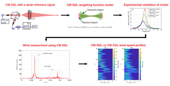
In this work, we demonstrate an improved CW DDL using a fiber-based sFPI and a Si-based SPC. The sFPI-DDL operates at 775 nm and has a large dynamic range of wind speed sensing (0 to 194 m/s or −97 m/s to +97 m/s). The spatial confinement of the sFPI-DDL probe volume is theoretically modeled by adopting the principle for calculation of the weighting function of a CW CDL. The efficacy of this model is also confirmed experimentally. We show that a CW DDL has a spatial sensitivity that is well approximated by a Lorentzian profile similar to that of a CW CDL. Moreover, wind detection at a 40 m range is carried out using the sFPI-DDL in side-by-side comparison with a CDL reference sensor. The wind profiles obtained by the two lidar systems show a high degree of agreement. We describe and emphasize how the reference signal irradiance in the sFPI-DDL is reduced sufficiently by using an improved design of the optical system that maintains low insertion loss to the received aerosol signal. Therefore, it achieves a much higher sensitivity than the sFPI-DDL of our previous work in [23]. In contrast to pulsed DDL systems [24,25], spatially resolved wind speed measurement is achieved by our CW DDL without the complexity associated with pulsed sources and timing electronics. To our best knowledge, the system we demonstrate here is the first CW DDL that enables remote wind sensing with both high spatial resolution (8 m) along its line of sight and high temporal resolution (<1 s). The wide dynamic speed range of the sFPI-DDL indicates its potential use in high-performance wind tunnels [9,10,26].
2. Spatial Confinement of the sFPI-DDL
Most of the DDL systems reported in the literature operated in a collimated lidar beam configuration [19,20,21,24,25]. Therefore, the lidar beam geometry has no significant influence on the weighting function of these DDL systems. The pulse duration of the pulsed laser defined the spatial resolution of these DDL systems. In contrast, the DDL demonstrated in this work employs a CW laser, and the spatial confinement (or spatial resolution) of the system depends on the overlap integral of the transmit and the receive beams—the area integral varies along the lidar beam propagation axis. In order to investigate the spatial confinement of a CW DDL, a theoretical model is derived first using the principle of the weighting function of a CW CDL as a guide. Secondly, the weighting function of the CW DDL with different overlap conditions for the transmit and the receive beams is measured experimentally, which also validates our model.
2.1. Theory
The calculation of the spatial confinement (or weighting function) of CDL systems has been discussed thoroughly in the literature [13,14,18]. Instead of analyzing the beat signal between the local oscillator and the backscattered signal on the detector plane, the concept of a virtual backpropagated local oscillator (BPLO) field was proposed. The spatial confinement can be understood as the axial variation in the overlap integral of the transmit beam and the BPLO beam transverse irradiances [18,27]. For example, if the transmit and BPLO beams are modeled as identical Gaussians, the axial weighting function takes the form of a Lorentzian. For the presented sFPI-DDL that utilizes a fiber to receive and guide signal photons to the sFPI and the detector, the local oscillator does not exist, but the concept of BPLO can still be borrowed by replacing the local oscillator with the transverse mode field of the fiber.
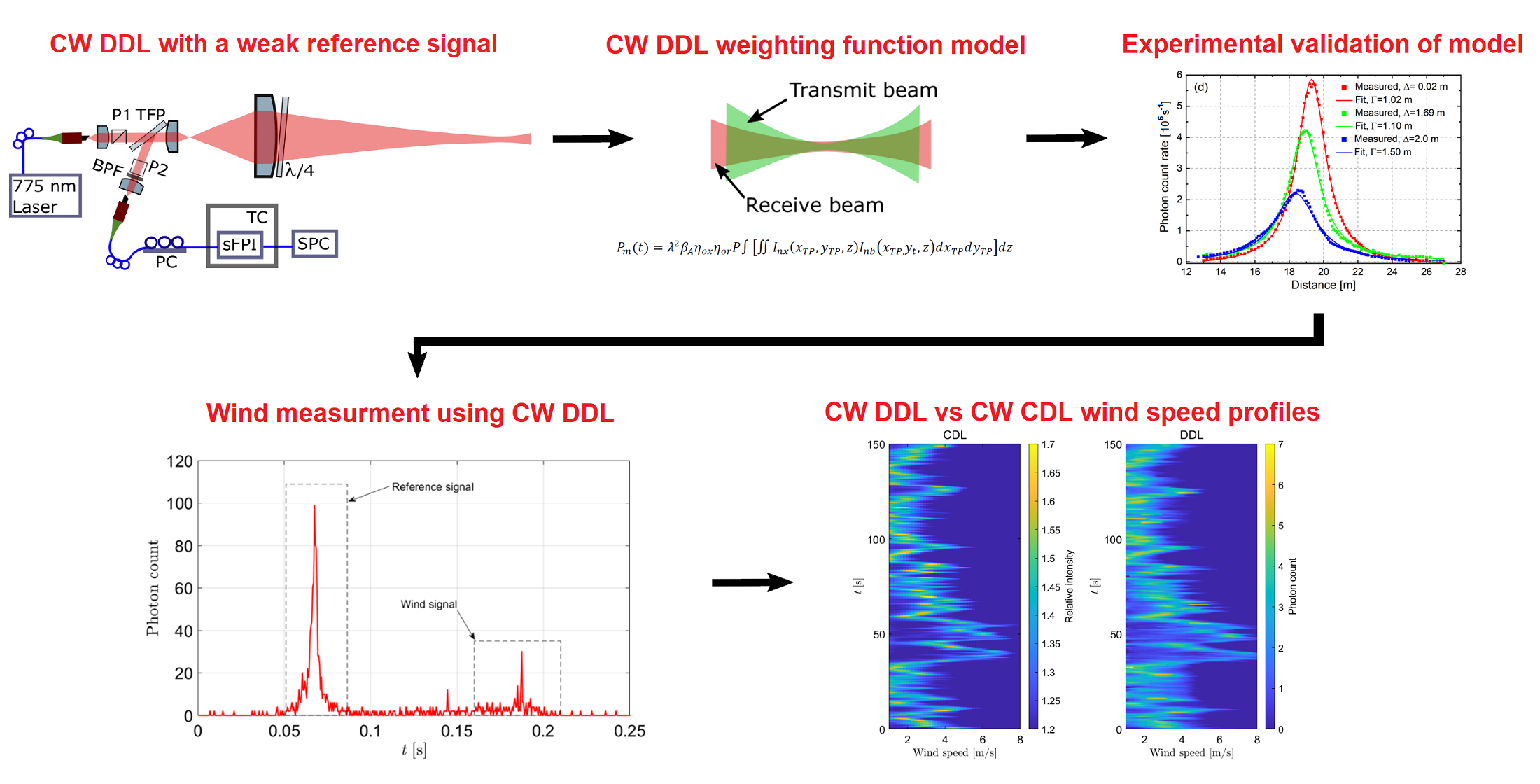
For a better understanding of the analogy between the local oscillator field in CDL and the fiber transverse mode field in DDL, Figure 1a,b show the simplified receivers of the CDL and DDL, respectively. In Figure 1a, the optical field of the backscattered signal (of power ) is mixed with the local oscillator (of power ) and the heterodyne signal strength is proportional to the degree of overlap between the fields of the backscattered signal and the local oscillator. Similarly, for the sFPI-DDL shown in Figure 1b, the signal strength is proportional to the power of the received signal field that is coupled into the fiber, i.e., the degree of overlap between the backscattered signal and the fiber mode.
Assuming a single-mode fiber is utilized for the sFPI-DDL receiver, the power of the backscattered signal coupled into the fiber [28] is
where is the complex amplitude of the signal field in the plane of the fiber entrance facet, and is the normalized transverse mode field of the fiber. Considering the backscatter from a single particle located at , can be written as [18]
where is the complex amplitude of the transmit field, is the scattering coefficient, is the wavenumber, is the speed of light, and the subscript denotes the target plane. Note that paraxial approximation is used in Equation (2).
Following the principle of BPLO in CDL [18], in sFPI-DLL can be backpropagated as
Thus, Equation (1) can be written as
where is the backscattering cross-section of the particle, and are the optical transmissions of the transmitter and the receiver, respectively. is the atmospheric transmission, is the laser power, and are the normalized irradiance profiles of the transmit beam and the backpropagated fiber mode (BPFM), respectively (normalized such that their area integrals prior to truncation by the lidar aperture of diameter D are both unity).
Based on Equation (4), the power of the lidar backscattered signal originating from a volume of random diffuse scatterers can be calculated by an integration over a volume:
where , is the volume density of the scattering centers in the atmosphere. For the case in which a CW laser is used,
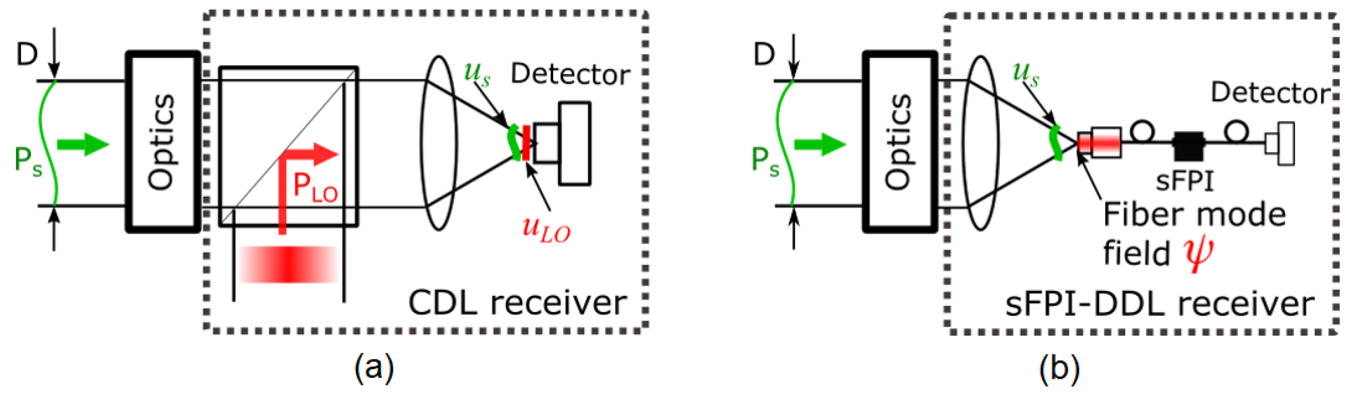
By considering the area (overlap) integral part of Equation (6), the spatial weighting functions of the sFPI-DDL with different alignment conditions are calculated and shown in Figure 2. It is assumed that both transmit and receive beams have Gaussian profiles and are focused by a 50 mm aperture lens without aberration. The normalized target-plane irradiances in Equation (6) are calculated numerically by following the approach implemented in [29]. The half width at half maximum of the weighting function is obtained by fitting the result with a Lorentzian function
where is the distance between the lidar and the target plane, , and are the fitting parameters, is where the fit is maximum. Figure 2a shows the weighting function for a transmit beam focused at 20 m. The receive beam is focused at either 20 m or a slightly shorter distance of (20 m − ). Both transmit and receive beams have the same truncation ratio = 0.8. is defined as the ratio of the (1/e2) Gaussian beam diameter 2 at the lidar aperture (pupil plane) and the diameter of the aperture [18]. As the spatial (axial) separation between the transmit and the receive beam waists increases, the weighting function broadens (i.e., increases ), and both its peak amplitude and peak position decrease. The simulation results in Figure 2b show the weighting function for cases where the transmit and receive beams have the same (red curve) or different (green curve) truncation ratios (both with = 0). In order to get the optimal weighting function that maximizes the volume integral of Equation (6), the two beams should both have a truncation ratio of 0.8—mimicking the Wang condition known to CDL systems [15].
Equation (6) has a similar form as the CDL signal-to-noise ratio [18]. Therefore, some important aspects about CDL systems can be adopted for the sFPI-DDL: good optical alignment of the transmit beam and the BPFM is necessary in order to maximize the return signal; analysis of the optimal truncation ratio of a monostatic sFPI-DDL is the same as that of the monostatic CDL [15,16]; optical aberrations in sFPI-DDL should be minimized in order to prevent significant broadening of the spatial confinement [11,29].
2.2. Experiments and Results
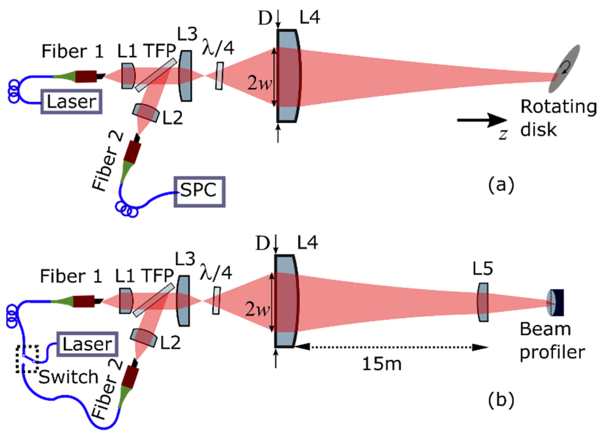
For both CDL and DDL, it is important to optimize the overlap between the optical axes of the transmit beam and the virtual backpropagated beam in order to maximize lidar sensitivity. However, the two lidar schemes also have a notable difference: for typical monostatic CDL systems, the transmit beam and the BPLO have the same normalized transverse irradiance profiles since the two beams originate from the same source (typically, a 1 mW LO is tapped from a 0.1% partial reflector while most laser power in the order of 1 W is transmitted through the CDL telescope). In sFPI-DDL, the normalized target-plane irradiances of the BPFM and the transmit beam generally differ because they do not originate from a single source. For the specific sFPI-DDL presented in this work, the target-plane irradiances of the transmit beam and the BPFM are influenced by the mode profiles at two separate fiber tips (Fiber 1 and Fiber 2) and their respective collimation lenses (L1 and L2) as shown in Figure 3a. Ideally, the optical field emitted from Fiber 1 and collimated by lens L1 should have the same wavefront curvature and diameter as the virtual backpropagated mode field of Fiber 2 and collimating lens L2 in order to optimize the spatial overlap. In practice, however, Fiber 1 and Fiber 2 of the same type (even from the same manufacturer) may still have slightly different mode field diameters (MFDs).
In order to investigate the effect of beam overlap on the weighting function of the sFPI-DDL, two experiments are designed and performed accordingly. To achieve optimal spatial overlap between the transmit beam and the BPFM, a monostatic lidar geometry is utilized in the experiments. Figure 3a shows the setup for measuring the weighting function of the sFPI-DDL. The output of a fiber-coupled external-cavity diode laser (ECDL, SWL-7513, Spectra-Physics, Milpitas, CA, USA) is collimated by lens L1. The operating wavelength of the ECDL is 780 nm and its power is stabilized at 0.3 mW. The beam waist diameter of the collimated beam is 1.8 mm. Using a telescope consisting of lenses L3 and L4, the beam is focused at a distance of 20 m from the pupil plane of lens L4. The hard target (a rotating disk) is placed at various axial positions between 13 m and 27 m from lens L4, and the target backscattered signal received by the telescope (lenses L3 and L4) is coupled into a fiber by lens L2. Note that the frequency discriminator is temporarily removed from the setup; only the power of the return signal is measured to obtain a profile of the spatial confinement or weighting function of the lidar system.
Figure 3b shows the setup for the characterization of the beam profile. The optical alignment remains the same as in Figure 3a, however, an optical switch is utilized in order to couple the laser into the transmit beam path and the receive beam path, alternately. The transmit beam emitted from Fiber 1 is the same as the one in Figure 3a, and its profile can be measured directly. Switching the laser to Fiber 2 to re-trace the receive beam path is essentially a realization of the BPFM. The transmit and the receive beams are focused by lens L5 placed 15 m away from lens L4, and the profile of the focused beam is measured by a beam profiler (BP209-VIS/M, Thorlabs) at different axial positions.
In the first experiment, Fiber 1 and Fiber 2 are of the same type (PM780-HP, MFD = 5 µm). The output beam from Fiber 1 is collimated by lens L1 and the distance between Fiber 1 and lens L1 is fixed for all the measurements. In contrast, the output beam from Fiber 2 is focused at different axial positions by changing the distance between the tip of Fiber 2 and lens L2. For different axial positions, the weighting functions and the beam profiles are measured accordingly.
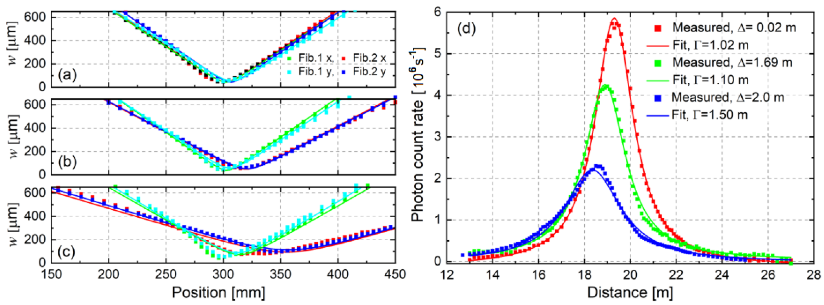
Figure 4a–c show three examples of the beam profiles measured by the setup in Figure 3b. By fitting the data to a model based on Gaussian beam propagation, the beam waist separations between the transmit beam and the BPFM focused by lens L5 are 0.2 mm (a), 16.9 mm (b) and 20.0 mm (c), respectively. Considering the demagnification introduced by lens L5 along the direction, i.e., (5 m/0.5 m)2 = 100 times reduction, the actual separation between the transmit beam and the BPFM (in the absence of lens L5) is 0.02 m, 1.69 m and 2.0 m, respectively. Figure 4d shows how the measured weighting function of the system varies as increases. In comparison to the simulation results shown in Figure 2a, the measured weighting function shows a similar trend of increasing , decreasing peak value and shifting (decreasing) peak position as increases. It is noteworthy to emphasize the following two points: (1) the measured weighting function is further broadened due to optical aberrations present in the optical system, which is not included in the simulations; (2) due to the presence of optical aberrations, the optimal truncation ratio is expected to be smaller than 0.8 [29]. Thus, with the available lenses and fibers in our laboratory, the truncation ratio for the transmit and the receive beam is designed as = = 0.63 for the case where both beams are focused at the same position—Figure 4a and the red curve in Figure 4d.
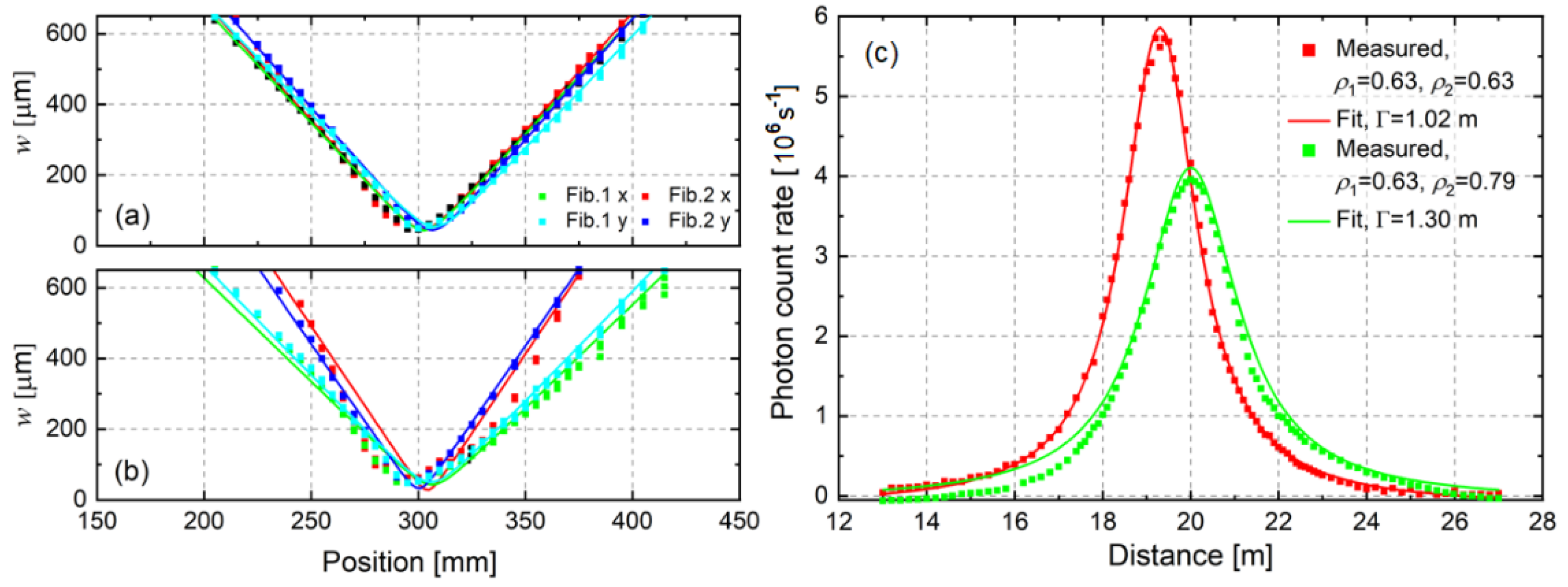
In order to investigate the effect of beam divergence on the weighting function of the sFPI-DDL, two types of fibers are used in the second experiment. Both transmit and receive beams are focused at ~20 m. The beam profiles and the weighting function are measured for the case where Fiber 1 and Fiber 2 have the same MFD—Figure 5a and red curve in Figure 5c; or different MFDs—Figure 5b and green curve in Figure 5c. If the two fibers are of the same type (PM780-HP, MFD = 5 μm), the divergences of the two beams are the same as shown in Figure 5a, and the truncation ratio for both beams can be calculated as = = 0.63. In contrast, if the two fibers are of different types (Fiber 1 is PM780-HP, Fiber 2 is HB800 with MFD = 4 μm), the divergences are different as shown in Figure 5b, and the truncation ratios for the transmit beam and the receive beam are = 0.63 and = 0.79, respectively. The measured weighting function is narrower for the case where the BPFM and transmit beam divergences are equal.
3. Wind Measurement Using sFPI-DDL
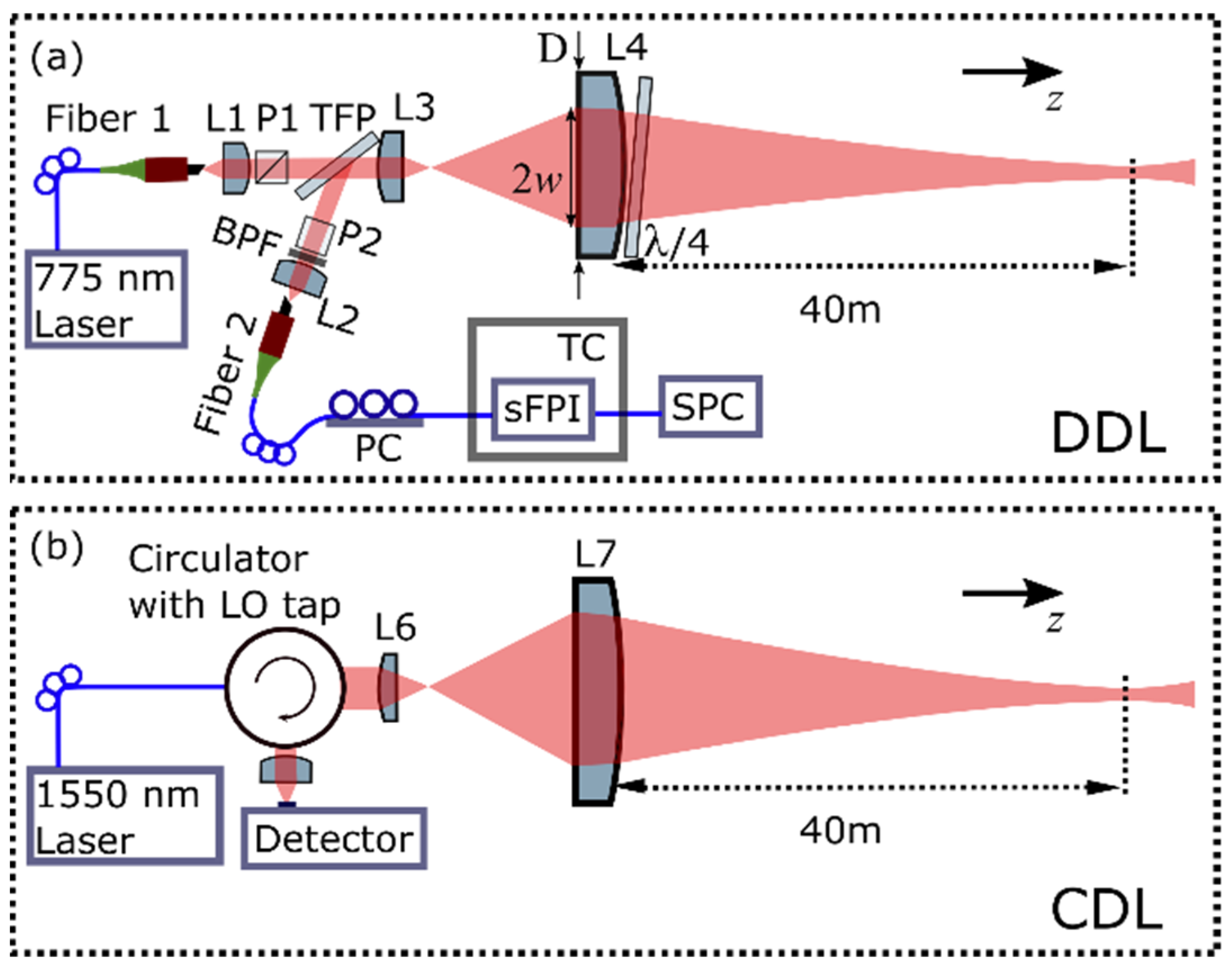
As mentioned in the introduction section, the detector noise of the sFPI-DDL in [22] was significantly reduced in [23] by changing the operating wavelength from 1.5 um to 787 nm to enable the use of a low-noise Si-based SPC. As a consequence, the relatively high reference signal strength became the limiting factor for improving the sensitivity of the system in [23]. In this work, further enhancements to the sFPI-DDL sensitivity were achieved by the reduction of the reference signal strength to a sufficient level. Figure 6a shows the setup of the sFPI-DDL. Most of the components are the same as in Figure 3a, but it is necessary to emphasize the following points: (1) Fiber 1 and Fiber 2 of the same type (PM780-HP) are used. (2) The power of the CW 775 nm laser is around 600 mW emitted from a frequency-doubled 1550 nm laser. The 1550 nm laser consists of a seed laser (RIO0195–3–02–3, RIO) and an erbium-doped fiber amplifier (CEFA–C–PB–HP–PM–37, KEOPSYS). The linewidth of the seed laser is 3.4 kHz, thus the linewidth of the 775 nm laser is less than 10 kHz or more than 100 times smaller than the spectral resolution of the fiber-based sFPI (~1 MHz). (3) The reference signal in Figure 3a mainly comes from the transmitted beam power reflected off the second anti-reflection coated surface of the quarter-wave (/4) plate. In order to reduce the irradiance of the reference signal, the small /4 plate between lenses L3 and L4 in Figure 3a is replaced with a 45 mm aperture /4 plate placed (with a slight tilt) after lens L4. In this new arrangement, the beam size on the /4 plate is larger, thus the reflection off the second surface of the /4 plate is coupled much less into Fiber 2, resulting in a weaker reference signal. (4) Two Glan–Taylor calcite polarizers (P1 and P2) are applied in the setup to reduce the reference signal strength further by improving the polarization extinction ratio of the transmit beam and the two receive beams (reference signal and wind signal). (5) The noise photons due to the ambient light are rejected by two band-pass filters (LL01–785–12.5 and LD01–785/10–12.5, Semrock) with an effective bandwidth of 3 nm. (6) The sFPI is placed in a box with a temperature controller in order to minimize scanning drifts due to temperature variation of the fiber-based sFPI. (7) The measured weighting function of the sFPI-DDL, i.e., the red curve in Figure 4d, shows that the spatial confinement width is 2 = 2.0 m for a lidar beam focused at 20 m distance. For the sFPI-DDL in Figure 6a with a lidar beam focused at 40 m, the spatial confinement width can be calculated as (2.0 m) (40 m/20 m)2 = 8.0 m.
In order to demonstrate the high sensitivity of this new sFPI-DDL, it was applied for wind measurement at a 40 m distance along with a CW CDL simultaneously. In the CDL setup shown in Figure 6b, the 1550 nm laser power is around 300 mW, its spatial confinement width is 5.0 m and the wind spectrum update rate is 50 Hz. The beams from the CDL and the DDL were parallel, pointed to the sky with an elevation angle of around 30° and were 1 m apart. The measurements were taken at the Roskilde campus of the Technical University of Denmark, on the 24 May 2021. The weather was partly cloudy.
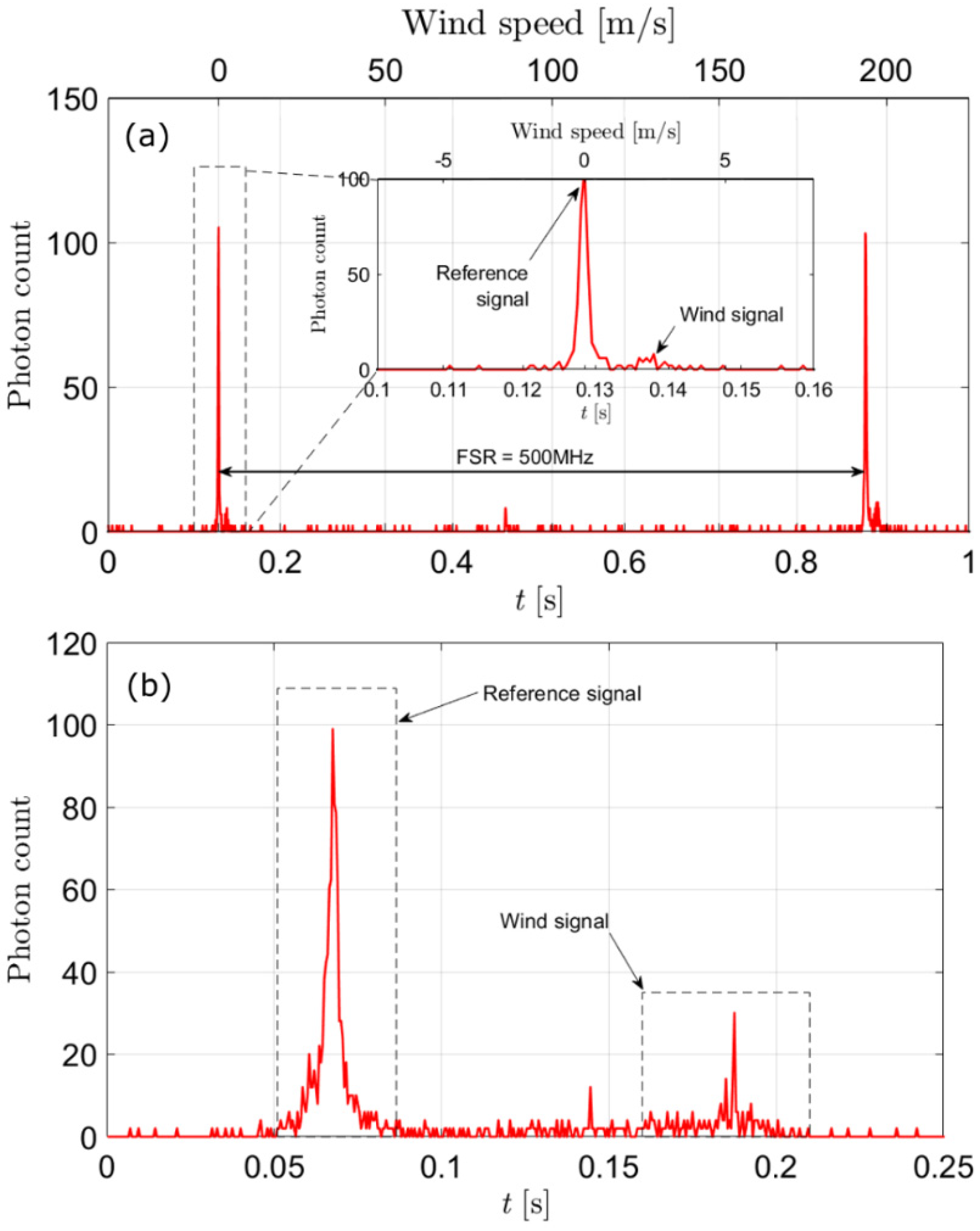
Figure 7a shows one example of the scanned signal from the sFPI-DDL with a scanning voltage = 6 V. Two temporally separated reference signals in Figure 7a indicate that one single scan with = 6 V can cover the free spectral range (FSR = 500 MHz) of the sFPI. The inset in Figure 7a shows the detail of the reference signal along with the wind signal, and the top axis of the plot corresponds to the wind speed magnitude , which is calculated using
where = 775 nm, is the temporal separation between the reference and the wind signal and is the temporal separation between two reference signals. The scanning rate was 1 Hz and the integration time for each bin was = 1 ms. In order to increase the scanning rate without compromising the strength of the wind signal, was decreased to 0.3 V. One typical scan with = 4 Hz and = 0.5 ms is shown in Figure 7b. Unlike in Figure 7a, only one reference signal is covered in Figure 7b. Equation (8) cannot be used to calculate the speed of the wind directly since is not available. Therefore, the mapping of speed from the time interval between the reference and the Doppler signal is calibrated with known speeds of a moving target (i.e., a rotating disk).
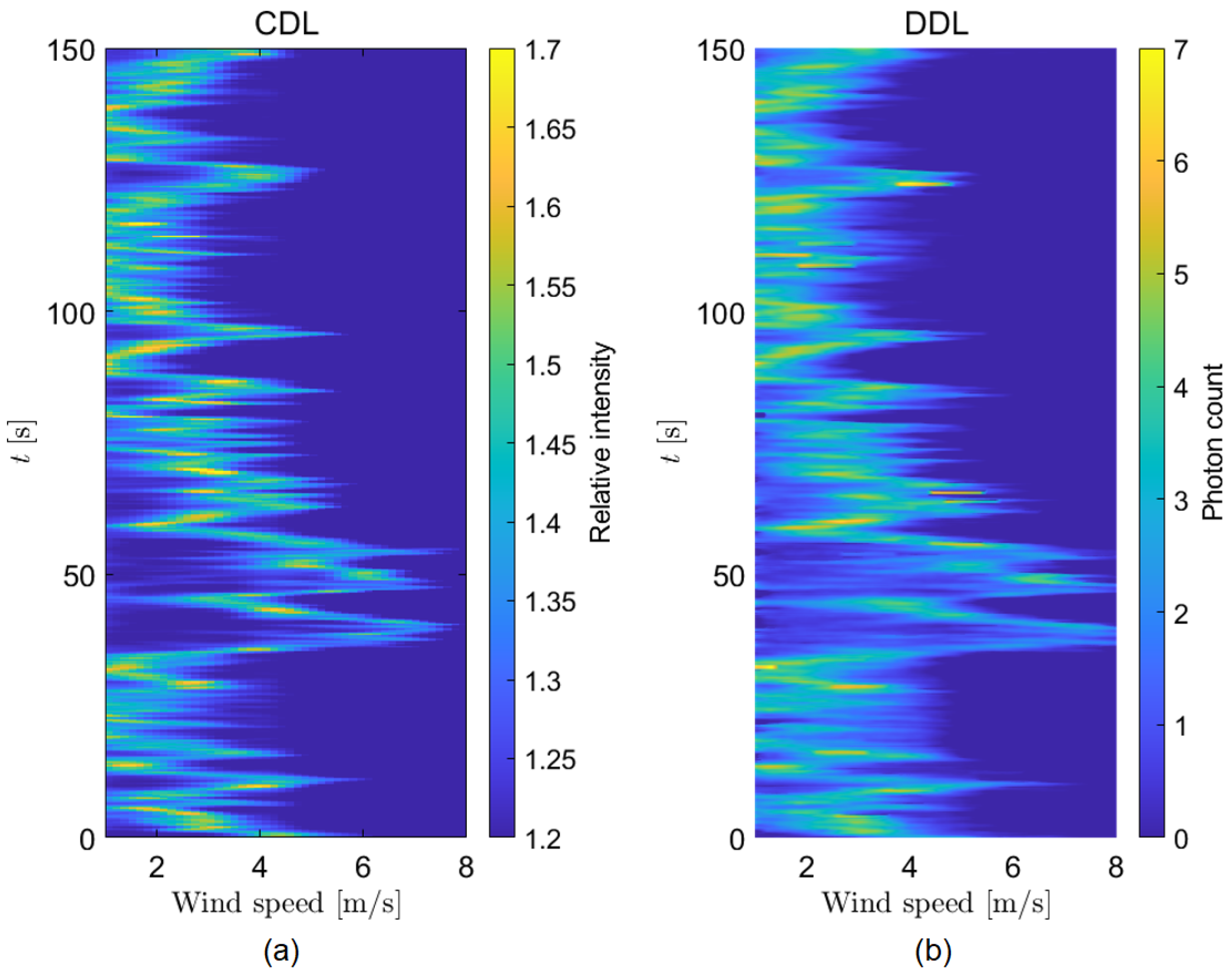
As an additional data processing step, the raw data are smoothed out using a moving average with a sliding window of 5 × 20 and 40 × 4 (wind speed bins × time bins) for the CDL and the DDL data, respectively. The post-processed wind profiles measured by the CDL and the sFPI-DDL, respectively, are presented in Figure 8. By comparing the variation of the two wind speed profiles over time, it can be concluded that the measurements provided by the CDL and the DDL are in reasonably good agreement. Potential sources of minor differences in the two wind profiles are the different actual probe positions (the lidar beams were not spatially overlapping) and the different of the two weighting functions. Figure 8 demonstrates the sufficient sensitivity and reliability of the sFPI-DDL for wind measurements with an update rate of 4 Hz.
4. Discussion
For our sFPI-DDL, the backscattered photons can only be detected if its optical frequency matches a resonance frequency of the sFPI, even though a CW laser is applied. More specifically, the wind signal only appears between 0.17 s and 0.19 s in Figure 7b; the photons in other time intervals are all rejected by the sFPI, i.e., more than 92% of the photons coupled into the sFPI cannot be registered as part of the detected wind signal. If a larger scanning voltage is applied, the losses would be even higher as shown in Figure 7a. In contrast, for the CDL measurement, the backscattered (and Doppler shifted) photons constantly mix with the local oscillator, and all contribute to the signal detection. This is one of the main reasons why the DDL has a lower signal-to-noise ratio than the CDL during the wind measurement. In order to improve the sensitivity and functionality of the CW DDL even further, the following five aspects may be considered.
- Truncation ratio
The truncation ratio of our sFPI-DDL is 0.63, which is not the optimal value of 0.8 especially if optical aberrations are minimized or absent [15,16,29]. It is also one of the reasons why the DDL has a broader weighting function compared with that of the CDL. It can be easily fixed by changing the focal length of lens L3 in Figure 6 a. Based on calculation of the antenna efficiency in [18], the sFPI-DDL signal is expected to be improved by ~5%.
- 2.
- Aperture of lens L4
Limited by the 45 mm aperture diameter of the /4 plate, a 2-inch lens L4 is used in Figure 6a. In principle, the sFPI-DDL can have the same aperture (3-inch) as the CDL by replacing lens L4 and the /4 plate with 3-inch versions. However, a 3-inch /4 plate could be very expensive. Instead, we suggest replacing the 2-inch lens L4 with a 3-inch lens with an appropriate focal length, and placing the current 45 mm /4 plate between L3 and L4 where the beam diameter is slightly smaller than 45 mm. In this way, more backscattered photons may be received by the larger aperture while the reference signal strength generated by the /4 plate would remain sufficiently low. Using a lens L4 with a larger diameter also improves the axial spatial resolution of the sFPI-DDL at the measurement distance of 40 m.
- 3.
- Transmission of the fiber-based sFPI
The finesse of the fiber-based sFPI is around 500 and its transmission at resonance frequency may be designed to reach if not exceed 50%. However, the measured transmission is only 8%. The extra loss is suspected to be due to the different fiber types (different MFDs and/or fiber tip cut angles) of the presently used Fiber 2 and the fiber comprising the sFPI. One solution would be coupling the backscattered signal into the sFPI directly without the extra fiber (Fiber 2). However, the use of Fiber 2 in the setup in Figure 3b proved to be useful in optimizing the spatial overlap of the transmit and receive beams of the sFPI-DDL. Thus, an alternative alignment procedure has to be formulated in the absence of Fiber 2.
- 4.
- Laser wavelength tuning
In the current sFPI-DDL, the frequency of the laser is stabilized and the transmission of the fiber-based FPI is tuned by changing the fiber length (the cavity length) with a piezo. However, the piezo inside the sFPI has a certain nonlinear response, which effectively results in the nonlinear response of the sFPI scan (especially over a full FSR) with a piezo ramp drive voltage. This explains why, in Figure 7a, the width of the left reference signal is slightly larger than that of the right one. Therefore, it is necessary to calibrate the nonlinearity of the sFPI before using it for accurate wind speed measurements, especially in a large dynamic speed range. In order to avoid this additional calibration process, tuning the frequency of the laser by changing the drive current of the laser is a promising alternative (and supports a faster response than piezo tuning). According to specifications of our seed laser, the current tuning coefficient is 3 pm/mA, which corresponds to 800 MHz/mA of the 775 nm laser. Thus, the central frequency of the laser can be tuned by 400 MHz by simply changing the current by 0.5 mA, so it can be expected to have a linear response in such a small tuning range in the laser drive current. Furthermore, replacing the sFPI with a fixed etalon will simplify the optical system. A fixed Fabry–Perot etalon is easier to temperature stabilize and has the potential for improving the on-resonance transmission (or optical throughput of the DDL), thus improving sensitivity and/or update rate for wind sensing.
- 5.
- Ranging capability
Pulsed DDL systems have ranging capability based on the time-of-flight of the laser pulse. In contrast, the CW DDL in this work can only measure the wind for a specific position (40 m away). The position of wind measurement is decided by the position at which the telescope focuses the lidar beam. A certain ranging capability in CW DDL can be achieved by simply changing the focus position of the lidar beam, for example, by a small axial displacement of lens L3 relative to lens L4 in Figure 6a. Although the probing range is readily adjustable without the added complexity of time-of-flight techniques, the probe length (2) of a CW DDL increases quadratically with probing range (like in a CW CDL [14]).
5. Summary
In this work, we have demonstrated a CW direct detection lidar using a fiber-based scanning Fabry–Perot interferometer for wind sensing. The spatial confinement of the sFPI-DDL was investigated both theoretically and experimentally. We showed that the sFPI-based CW DDL has a Lorentzian weighting function. Note that prior to this work, spatial confinement in an sFPI-DDL wind sensor has only been achieved by using pulsed lasers [24,25]. We derived a simple model for calculating the weighting function of the fiber-based sFPI-DDL. This model successfully explained the broadening mechanism of the spatial confinement observed in our experiments. Moreover, we improved the sensitivity of the CW DDL by lowering the noise from the reference signal with a new and simple optical design. This enabled the application of CW DDL for actual wind measurement for the first time. The sFPI-DDL was applied to measure the wind 40 m away with an update rate of 4 Hz along with a CW CDL simultaneously. The two wind lidar systems showed good consistency in their measurement results, which validates the sensitivity of the sFPI-DDL experimentally. In summary, this type of DDL shows great application prospects for remote wind velocimetry with sign discrimination, especially for applications in which a compact system with a high dynamic range of wind speed and spatially resolved measurement is needed (e.g., wind sensing in a large wind tunnel [26]).
Author Contributions
Conceptualization, C.P. and P.J.R.; methodology, L.M., C.P. and P.J.R.; software, L.M.; validation, L.M. and P.J.R.; formal analysis, L.M.; investigation, L.M.; data curation, L.M.; writing—original draft preparation, L.M.; writing—review and editing, C.P. and P.J.R.; visualization, L.M.; supervision, P.J.R.; project administration, C.P. and P.J.R.; funding acquisition, C.P. and P.J.R. All authors have read and agreed to the published version of the manuscript.
Funding
Innovation Fund Denmark (Grant no. 8054-00050B).
Conflicts of Interest
The authors declare no conflict of interest.
References
- Manninen, A.J.; Marke, T.; Tuononen, M.J.; O’Connor, E.J. Atmospheric boundary layer classification with Doppler lidar. J. Geophys. Res. Atmos. 2018, 123, 8172–8189. [Google Scholar] [CrossRef]
- Prasad, N.S.; Tracy, A.; Vetorino, S.; Higgins, R.; Sibell, R. Innovative fiber-laser architecture-based compact wind lidar. In Photonic Instrumentation Engineering III; International Society for Optics and Photonics: Bellingham, WA, USA, 2016; Volume 9754, p. 97540J. [Google Scholar]
- Wu, S.; Zhai, X.; Liu, B. Aircraft wake vortex and turbulence measurement under near-ground effect using coherent Doppler lidar. Opt. Express 2019, 27, 1142–1163. [Google Scholar] [CrossRef] [PubMed]
- Smalikho, I.N.; Köpp, F.; Rahm, S. Measurement of atmospheric turbulence by 2-μm Doppler lidar. J. Atmos. Ocean. Technol. 2019, 22, 1733–1747. [Google Scholar] [CrossRef]
- Peña, A.; Mann, J. Turbulence measurements with dual-Doppler scanning lidars. Remote Sens. 2019, 11, 2444. [Google Scholar] [CrossRef] [Green Version]
- Shimada, S.; Goit, J.P.; Ohsawa, T.; Kogaki, T.; Nakamura, S. Coastal wind measurements using a single scanning LiDAR. Remote Sens. 2020, 12, 1347. [Google Scholar] [CrossRef] [Green Version]
- Shun, C.M.; Chan, P.W. Applications of an infrared Doppler lidar in detection of wind shear. J. Atmos. Ocean. Technol. 2008, 25, 637–655. [Google Scholar] [CrossRef]
- Beuth, T.; Fox, M.; Stork, W. Parameterization of a geometrical reaction time model for two beam nacelle lidars. In Lidar Remote Sensing for Environmental Monitoring XV; International Society for Optics and Photonics: Bellingham, WA, USA, 2015; Volume 9612, p. 96120J. [Google Scholar]
- van Dooren, M.F.; Campagnolo, F.; Sjöholm, M.; Angelou, N.; Mikkelsen, T.; Kühn, M. Demonstration and uncertainty analysis of synchronised scanning lidar measurements of 2-D velocity fields in a boundary-layer wind tunnel. Wind Energy Sci. 2017, 2, 329–341. [Google Scholar] [CrossRef] [Green Version]
- Iungo, G.V. Experimental characterization of wind turbine wakes: Wind tunnel tests and wind LiDAR measurements. J. Wind Eng. Ind. Aerod. 2016, 149, 35–39. [Google Scholar] [CrossRef]
- Rye, B.J. Primary aberration contribution to incoherent backscatter heterodyne lidar returns. Appl. Opt. 1982, 21, 839–844. [Google Scholar] [CrossRef] [PubMed]
- Frehlich, R.G.; Kavaya, M.J. Coherent laser radar performance for general atmospheric refractive turbulence. Appl. Opt. 1991, 30, 5325–5352. [Google Scholar] [CrossRef]
- Sonnenschein, C.M.; Horrigan, F.A. Signal-to-noise relationships for coaxial systems that heterodyne backscatter from the atmosphere. Appl. Opt. 1971, 10, 1600–1604. [Google Scholar] [CrossRef] [PubMed]
- Hill, C. Coherent Focused Lidars for Doppler Sensing of Aerosols and Wind. Remote Sens. 2018, 10, 466. [Google Scholar] [CrossRef] [Green Version]
- Wang, J.Y. Optimal truncation of a lidar transmitted beam. Appl. Opt. 1988, 27, 4470–4474. [Google Scholar] [CrossRef]
- Rye, B.J.; Frehlich, R.G. Optimal truncation and optical efficiency of an apertured coherent lidar focused on an incoherent backscatter target. Appl. Opt. 1992, 31, 2891–2899. [Google Scholar] [CrossRef]
- Zhao, Y.; Post, M.J.; Hardesty, R.M. Receiving efficiency of pulsed coherent lidars. 1: Theory. Appl. Opt. 1990, 29, 4111–4119. [Google Scholar] [CrossRef]
- Fujii, T.; Fukuchi, T. Laser Remote Sensing, 1st ed.; CRC Press Taylor: Boca Raton, FL, USA; Francis Group: Abingdon, UK, 2005; pp. 469–722. [Google Scholar]
- Xia, H.Y.; Sun, D.S.; Yang, Y.H.; Shen, F.H.; Dong, J.J.; Kobayashi, T. Fabry-Perot interferometer based Mie Doppler lidar for low tropospheric wind observation. Appl. Opt. 2007, 46, 7120–7131. [Google Scholar] [CrossRef] [PubMed] [Green Version]
- Liu, Z.; Liu, B.; Li, Z. Wind measurements with incoherent Doppler lidar based on iodine filters at night and day. Appl. Phys. B 2007, 88, 327–335. [Google Scholar] [CrossRef]
- McKay, J.A. Assessment of a multibeam Fizeau wedge interferometer for Doppler wind lidar. Appl. Opt. 2002, 41, 1760–1767. [Google Scholar] [CrossRef] [PubMed]
- Rodrigo, P.J.; Pedersen, C. Monostatic coaxial 1.5 μm laser Doppler velocimeter using a scanning Fabry-Perot interferometer. Opt. Express 2013, 21, 21105–21112. [Google Scholar] [CrossRef] [Green Version]
- Rodrigo, P.J.; Pedersen, C. Direct detection Doppler lidar using a scanning Fabry-Perot interferometer and a single-photon counting module. In Proceedings of the European Conference on Lasers and Electro-Optics-European Quantum Electronics Conference, Munich, Germany, 21–25 June 2015; p. CH_P_15. [Google Scholar]
- Shangguan, M.; Xia, H.; Wang, C.; Qiu, J.; Shentu, G.; Zhang, Q.; Dou, X.; Pan, J.W. All-fiber upconversion high spectral resolution wind lidar using a Fabry-Perot interferometer. Opt. Express 2016, 24, 19322–19336. [Google Scholar] [CrossRef]
- Xia, H.; Shangguan, M.; Wang, C.; Shentu, G.; Qiu, J.; Zhang, Q.; Dou, X.; Pan, J. Micro-pulse upconversion Doppler lidar for wind and visibility detection in the atmospheric boundary layer. Opt. Lett. 2016, 41, 5218–5221. [Google Scholar] [CrossRef] [PubMed] [Green Version]
- Pedersen, A.T.; Montes, B.F.; Pedersen, J.E.; Harris, M.; Mikkelsen, T. Demonstration of short-range wind lidar in a high- performance wind tunnel. In Proceedings of the EWEA 2012, Copenhagen, Denmark, 16–19 April 2012. [Google Scholar]
- Siegman, A.E. The antenna properties of optical heterodyne receivers. Appl. Opt. 1966, 5, 1588–1594. [Google Scholar] [CrossRef] [PubMed]
- Winzer, P.J.; Leeb, W.R. Fiber coupling efficiency for random light and its applications to lidar. Opt. Lett. 1998, 23, 986–988. [Google Scholar] [CrossRef] [PubMed]
- Hu, Q.; Rodrigo, P.J.; Iversen, T.F.Q.; Pedersen, C. Investigation of spherical aberration effects on coherent lidar performance. Opt. Express 2013, 21, 25670–25676. [Google Scholar] [CrossRef] [Green Version]
Figure 1.
Functional diagram of the receiver for (a) CDL and (b) sFPI-DDL.

Figure 2.
Calculated spatial weighting functions of the sFPI-DDL. (a) The transmit beam and the receive beam (or BPFM) are focused at axial positions with spatial separation of ; (b) the transmit and receive beams are focused at the same position with either equal or unequal divergences.
Figure 2.
Calculated spatial weighting functions of the sFPI-DDL. (a) The transmit beam and the receive beam (or BPFM) are focused at axial positions with spatial separation of ; (b) the transmit and receive beams are focused at the same position with either equal or unequal divergences.

Figure 3.
Schematic layout of the experimental setups for (a) the weighting function measurement of the sFPI-DDL (the frequency discriminator, sFPI, is temporarily removed) and (b) the transmit and receive (BPFM) beam characterization. TFP, thin film polarizer; SPC, single photon counter; L1, L2, aspheric lenses, focal length f = 11 mm; L3, aspheric lens, f = 10 mm; L4, 2-inch achromatic lens, f = 150 mm; L5, singlet lens, f = 500 mm;, quarter-wave plate.

Figure 4.
Beam radii in the x and y directions of the transmit (Fiber 1) and the receive (Fiber 2) beams focused by lens L5 for cases where the waist positions of the two beams (without lens L5) are separated along the direction by (a) = 0.02 m, (b) = 1.5 m and (c) = 2 m. (d) Measured weighting functions (and fitting results) for different separation values between the transmit and the receive beam waists.

Figure 5.
Beam radii in the x and y directions of the transmit (Fiber 1) and the receive (Fiber 2) beams focused by lens L5 for (a) identical fibers (both MFDs = 5 µm) and (b) different fibers (MFD = 5 µm for Fiber 1; MFD = 4 µm for Fiber 2). (c) Measured weighting functions (and fitting results) for cases of two identical fibers (equal truncation ratios) and two different fibers (unequal truncation ratios).

Figure 6.
Schematic layout of the experimental setups for wind measurement using (a) CW sFPI-DDL and (b) CW CDL. PC, polarization controller. P1, P2, calcite linear polarizers. BPF, band-pass filter. sFPI, scanning Fabry–Perot interferometer. TC, temperature controller. LO, local oscillator. L6, aspheric lens. L7, 3-inch achromatic lens.

Figure 7.
Example of the sFPI-DDL raw data for a single scan. (a) = 1 Hz, = 1 ms, = 6 V. The inset shows the details around the signal. (b) = 4 Hz, = 0.5 ms, = 0.3 V.
Figure 7.
Example of the sFPI-DDL raw data for a single scan. (a) = 1 Hz, = 1 ms, = 6 V. The inset shows the details around the signal. (b) = 4 Hz, = 0.5 ms, = 0.3 V.

Figure 8.
The 150 s wind profiles measured by (a) the CDL and (b) the sFPI-DDL simultaneously. For sFPI-DDL, = 4 Hz, = 0.5 ms and = 0.3 V were used. A moving average with a sliding window (speed bins × time bins) of 5 × 20 was used for the CDL data (40 × 4 for the DDL data).
Figure 8.
The 150 s wind profiles measured by (a) the CDL and (b) the sFPI-DDL simultaneously. For sFPI-DDL, = 4 Hz, = 0.5 ms and = 0.3 V were used. A moving average with a sliding window (speed bins × time bins) of 5 × 20 was used for the CDL data (40 × 4 for the DDL data).

Publisher’s Note: MDPI stays neutral with regard to jurisdictional claims in published maps and institutional affiliations. |
© 2021 by the authors. Licensee MDPI, Basel, Switzerland. This article is an open access article distributed under the terms and conditions of the Creative Commons Attribution (CC BY) license (https://creativecommons.org/licenses/by/4.0/).
Share and Cite
MDPI and ACS Style
Meng, L.; Pedersen, C.; Rodrigo, P.J. CW Direct Detection Lidar with a Large Dynamic Range of Wind Speed Sensing in a Remote and Spatially Confined Volume. Remote Sens. 2021, 13, 3716. https://0-doi-org.brum.beds.ac.uk/10.3390/rs13183716
AMA Style
Meng L, Pedersen C, Rodrigo PJ. CW Direct Detection Lidar with a Large Dynamic Range of Wind Speed Sensing in a Remote and Spatially Confined Volume. Remote Sensing. 2021; 13(18):3716. https://0-doi-org.brum.beds.ac.uk/10.3390/rs13183716
Chicago/Turabian StyleMeng, Lichun, Christian Pedersen, and Peter John Rodrigo. 2021. "CW Direct Detection Lidar with a Large Dynamic Range of Wind Speed Sensing in a Remote and Spatially Confined Volume" Remote Sensing 13, no. 18: 3716. https://0-doi-org.brum.beds.ac.uk/10.3390/rs13183716
Note that from the first issue of 2016, this journal uses article numbers instead of page numbers. See further details here.