
Deep Learning for Chlorophyll-a Concentration Retrieval: A Case Study for the Pearl River Estuary


1
State Key Laboratory of Tropical Oceanography, South China Sea Institute of Oceanology, Chinese Academy of Sciences, Guangzhou 510000, China
2
Southern Marine Science and Engineering Guangdong Laboratory (Guangzhou), Guangzhou 510000, China
3
South China Sea Marine Prediction Center, State Ocean Administration, Guangzhou 510000, China
4
Key Laboratory of Marine Environmental Survey Technology and Application, Ministry of Natural Resources, MNR, Guangzhou 510000, China
5
Guangdong Provincial Key Laboratory of Marine Resources and Coastal Engineering, Sun Yat-sen University, Guangzhou 510000, China
*
Author to whom correspondence should be addressed.
Remote Sens. 2021, 13(18), 3717; https://0-doi-org.brum.beds.ac.uk/10.3390/rs13183717
Submission received: 9 August 2021
/
Revised: 5 September 2021
/
Accepted: 16 September 2021
/
Published: 17 September 2021
(This article belongs to the Section Ocean Remote Sensing)
Abstract
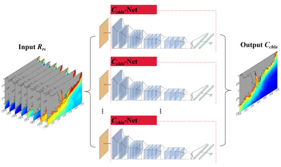
:The abundance of phytoplankton is generally estimated by measuring the chlorophyll-a concentration (Cchla), which is an important factor in photosynthesis and can be used to analyze the density and biomass of phytoplankton in the ecosystem. The band-ratio-based empirical or semi-analytical algorithms are operationally applied to retrieve Cchla in global oceans, which generally experience difficulties from the diversity of optical properties and the complexity of the radiative transfer equations in analytical analyses, respectively. With an attempt to develop an accurate Cchla retrieval model for the optically complex coastal and estuarine waters, this study aimed to explore the deep learning (DL) methods in satellite retrieval of Cchla. A two-stage convolutional neural network (CNN), named Cchla-Net, was proposed, which utilized the spectral information of remote sensing reflectances at MODIS/Aqua’s visible bands. In the first-stage phase, the Cchla-Net was pretrained by a set of remote sensing patches, in which the Cchla was generated from an existing model (OC3M). The pretrained results were than used as the initial values to refine the network with the synthetic oversampled in-situ dataset in the second-stage training phase. Using in-situ samples for training with the new initial values has a higher probability to reach the global optimum. The quantitative analyses showed that the two-stage training was more likely to achieve a global optimum in the optimization than the one-stage training. Matchups of the in-situ Cchla measurements were used to evaluate the retrieval models. Results showed that the proposed Cchla-Net produced obvious better performance than the empirical and semi-analytical algorithms, implying the DL method was more effective for optically complex waters with extremely high Cchla. This study provided an applicable method for remote sensing retrieval of Cchla, which should be helpful for studying the spatial distribution and temporal variability in the productive Pearl River estuary (PRE) waters.
1. Introduction
Chlorophyll-a concentration (Cchla) is one of the key estuarine water quality parameters and serves as an essential indicator of ocean primary productivity [1]. Accurate retrieval of Cchla from ocean color data is often an extremely challenging task in estuarine and coastal waters, due to the complex optical properties related to the inconstant and uncorrelated phytoplankton biomass, suspended sediments and colored dissolved organic matter (CDOM). The currently available satellite-derived water quality products are restricted to optically significant materials [2], and the standard ocean algorithms have tended to be largely dispersed in specific regions [3]. In addition, the atmospheric correction errors can lead to inaccuracies in remote sensing reflectance, especially for blue wavelengths, from which Cchla is typically derived [4]. Many retrieval models for Cchla estimation have been developed for different ocean color sensors, such as the sea-viewing wide field-of-view sensor (SeaWiFS), the moderate resolution imaging spectroradiometer (MODIS) and the visible infrared imaging radiometer suite (VIIRS). In general, the retrieval models are inputted with normalized water-leaving radiance (nLw) or remote sensing reflectance (Rrs) and compute Cchla in a direct or indirect way, and they can be grouped as empirical and semi-analytical models. Empirical models are commonly based on the band ratios of Rrs and regression functions [5,6,7]. The accuracy of empirical models mainly depends on the in-situ measurements utilized on their respective developments. Semi-analytical models [8,9] require analytical expressions relating inherent optical properties (IOPs) or apparent optical properties (AOPs) and several mathematical constraints. Semi-analytical models have advantages over the empirical models since they can derive multiple optical properties from a single water-leaving radiance spectrum. However, the relative complexity of the semi-analytical models has stalled the operational implementation since the optimal model parameters are hard to determine [10,11].
Machine learning methods have demonstrated their abilities in remote sensing applications, such as evapotranspiration estimates [12,13], and oceanic particulate organic carbon retrieval [14]. Deep learning (DL) methods, which exclusively learn the representative features in a hierarchical manner from data, have been recently introduced into the remote sensing community for big data analysis [15]. As the most representative supervised DL model, convolutional neural networks (CNNs) have proven to be good at extracting features from remote sensing imageries by interleaving convolutional and pooling layers [16]. The main advantages of CNNs are the association with nonlinear complexities, the reduced sensitivity to noise, and the ability to learn highly abstract features. Recent studies showed that CNNs were highly effective in large-scale image recognition and object detection [17,18,19,20,21]. For the Pearl River estuary (PRE), which has turbid and highly productive waters, several local algorithms for Cchla retrieval have been developed [22,23]. However, the DL network has not been widely applied to the PRE waters.
This study aimed to explore the potentials of DL in improving remote sensing retrieval of estuarine and coastal Cchla. To achieve the goal, with climatological monthly products from MODIS/Aqua ocean color data and long-term in-situ measurements, a two-stage CNN model, which was named Cchla-Net, was trained and validated by a k-fold cross-validation, and it was further compared with the representative empirical and semi-analytical models. The proposed network could contribute to developing more accurate Cchla retrieval approach in the turbid and high productive estuarine and coastal waters. By applying the network, the long-term Cchla products in the PRE were derived, from which the spatial distribution and the temporal variability were analyzed, and the different patterns were observed in the coastal and continental shelf area, which related to the river discharge, and the mixing of the upper layer was revealed.
2. Materials and Methods
2.1. Study Area
The PRE is a subtropical and high biological productivity estuary located in the continental shelf of the northern South China Sea (SCS). The SCS is a typical monsoon-influenced region. Southwest winds prevail in summer, and northeast winds prevail in winter [24,25]. In this study, the seasons refer to those for the northern hemisphere, i.e., summer refers to June, July and August, and winter refers to December, next January and February. As the third largest river in China, the Pearl River is well known for its complex river networks, and the water composition varies widely both spatially and temporally in the PRE [26]. Lingdingyang Bay of the Pearl River estuary (LBPRE) forms the largest estuarine bay in South China, which is a trumpet-shaped bay stretching in a near NNW-SSE direction and covering a sea area of about 2110 km2 [27]. With rapid growth of the population and urbanization, the PRE is contaminated by industrial pollution, agricultural runoff and domestic sewage, which threaten the water quality of the PRE [28,29]. In the study area, there are turbid and high productive coastal waters and clear continental shelf waters. As a result, the Cchla is characterized by wide ranges and fast changes, indicating that the PRE is a suitable place for training a representative retrieval network.
2.2. Data Sources
2.2.1. In-Situ Dataset
Ten campaigns were conducted between the year 2003 and 2012 to collect the water samples and optical spectrum. A total of 18 consistent stations were pre-set along the central y-axis of the PRE. The distance between neighboring stations was about 4.5 km, and all the stations covered a total distance of about 80 km from the sea upstream. Positions for sampling stations are plotted in Figure 1. Note that it only covered the first 16 or 17 stations in several campaigns due to weather conditions. A total of 165 in-situ Rrs and the corresponding Cchla dataset was collected. The statistical descriptions of the in-situ samples are summarized in Table 1.
The water-leaving Rrs was measured using a spectrometer (USB4000, Ocean Optics, Inc., Dunedin, FL, USA) following the National Aeronautics and Space Administration (NASA) ocean optics standard protocol [30]. The upwelling radiance (Lu), sky radiance (Lsky) and radiance reflected by a standard gray plaque (Lp) were measured, and Rrs was calculated using the following equation:
where λ is the wavelength, ρp is the reflectance of the gray plaque and ρf is the water surface Fresnel reflectance, with a value of 0.028 for wind speeds less than 5 m·s−1.
The water samples for measuring Cchla were collected from the surface layer (a depth of between 30 cm and 50 cm) and filtered through 25-mm Whatman GF/F filters under a low vacuum. The filters were measured using a 90% acetone method in a pre-calibrated Turner Design 10 fluorometer [31].
2.2.2. MODIS Imagery
Level-1A MODIS data onboard the Aqua spacecraft was obtained from the National Aeronautics and Space Agency (NASA) ocean color data archive. The remote sensing imageries were preprocessed using the SeaWiFS data analysis system (SeaDAS, version 7.5.3). The Management Unit of the North Seas Mathematical Models (MUMM) was employed for atmospheric correction [32]. Flags were used to mask contamination from land, clouds, sun glint and other potential disturbances. For the matchups between in-situ and satellite data, the procedure developed by Evers-King et al. was adopted [33]. A 3×3 box surrounding the location of the in-situ measurement was used to extract satellite data. The mean value within the box was calculated for each parameter if the box contained at least 3 valid pixels.
The discrepancies between in-situ measured and sensor-observed Rrs were minimized through the adjustment process based on a multilinear regression algorithm (MLR) [34]. The adjusted Rrsadj(λ) was calculated as follows:
where Rrsor(λ) is the original MODIS-observed Rrs, and ΔRrs(λ) is the discrepancy between in-situ measured and MODIS-observed Rrs. The MLR scheme is as follows:
where the input vectors are the original Rrs at the MODIS’s visible bands (412, 443, 469, 488, 547, 555, 645, 667 and 678 nm). The coefficients aisat (i = 0,1,...,9) were calculated through a multilinear regression between ΔRrs(λ) and the input vectors based on the matchup Rrs dataset.
3. Algorithm Development
3.1. Overall Framework
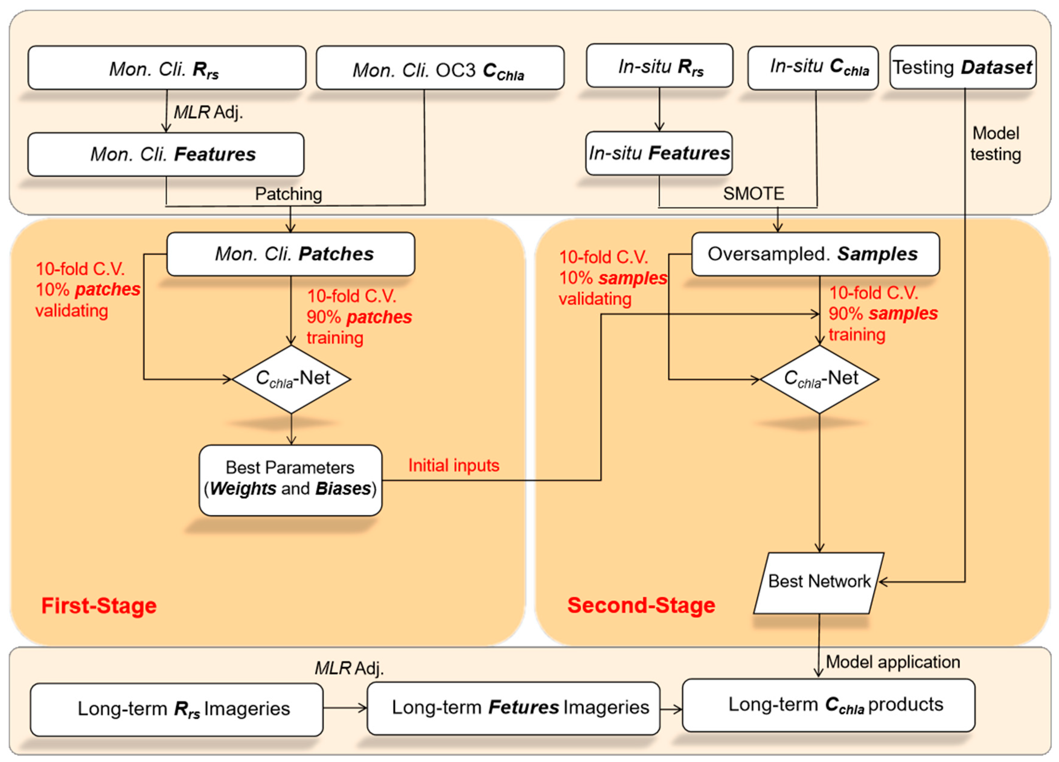
Despite the complex hierarchical structures, all the DL-based models included three main components: the prepared input data, the core deep networks and the expected output data. The overall framework is briefly outlined in Figure 2. Four major steps were involved in the development of network, including feature generation, imagery patching, dataset oversampling and two-stage Cchla-Net training and validating. In these steps, Rrs at the MODIS/Aqua’s visible bands were used to generate six sensitive features. The Ocean Colour 3 band ratio (OC3M) [4], a fourth-order band ratio algorithm that uses one of two blue and green band ratios, depending on the optical properties of different water types, was utilized for the initial Cchla estimation. The formula of OC3M is defined as follows:
A two-stage network was adopted to achieve a global optimum in the optimization. A synthetic minority oversampling technique was adopted to overcome the shortcoming of limited in-situ samples. The 10-fold cross-validation was applied for model training and validation. When the core deep network has been well-trained, it can be employed to predict the expected output of a given testing dataset.
The coefficient of determination (R2), root mean squared difference (RMSD), mean absolute difference (MAD) and mean absolute percentage difference (MAPD) between two datasets were used to evaluate model performance.
Here, xm and xp denote the measured and predicted samples, respectively. denotes the mean value of the measured samples, and N is the number of samples.
3.2. Feature Generation and Data Preprocessing
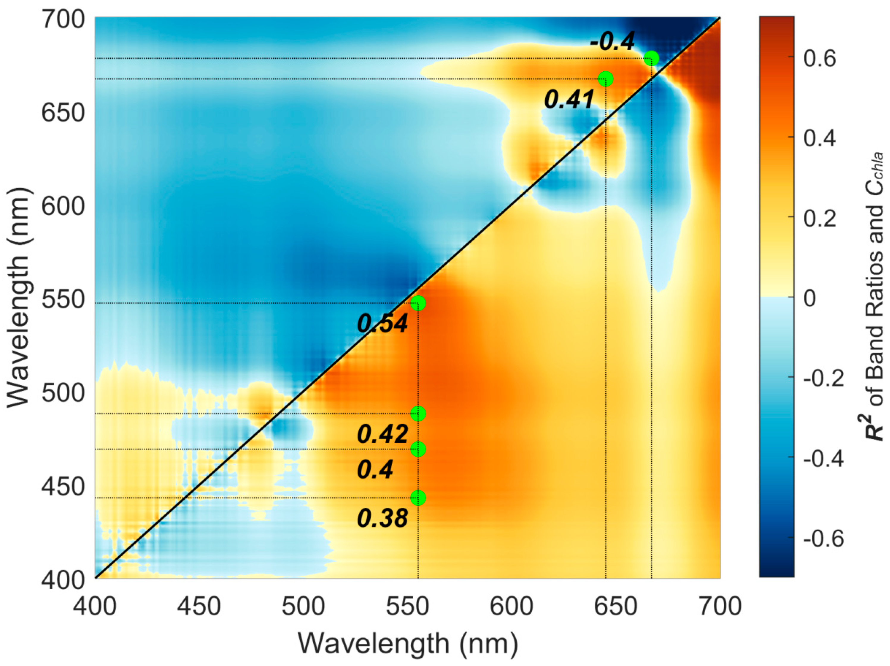
The atmospheric-corrected and adjusted Rrs at MODIS/Aqua’s visible bands were considered for algorithm development. Band ratio algorithms involving Rrs at blue and green bands have been widely employed for Cchla retrieval [4,6,7]. To determine the optimal band ratios for the PRE waters, Figure 3 shows the R2 from the linear regression analysis between different band ratios and Cchla based on in-situ dataset. It can be seen that the correlation was insufficient with those band ratios involving Rrs(412), which might be attributed to the atmospheric correction issues associated with the 412 nm band in turbid coastal waters. To improve the efficiency of Cchla-Net, six different band ratios, with R2 ranging from 0.38 to 0.54, were used as input features. The six band ratios were Rrs(443)/Rrs(555), Rrs(469)/Rrs(555), Rrs(488)/Rrs(555), Rrs(547)/Rrs(555), Rrs(667)/Rrs(645) and Rrs678)/Rrs(667).
The patching process was primarily performed to create a local 64 × 64 patch. The determination of patch size was a key procedure, which needed to take into account both the network’s structure and characteristics of the remote sensing imagery (i.e., spatial resolution). Features extracted from too small of a patch were insufficient for a deep network, whereas a single pixel’s Cchla from too large of a patch was not representative. Those patches with clouds or lands were eliminated. The maximum of the OC3M-based Cchla within the patch was used to represent the rough value of each patch. After the patching process, the log10-transformed Cchla and six band ratio data were normalized to 0.0~1.0 to ensure that they were in the same range.
3.3. Oversampling In-Situ Dataset
Cchla-Net is a deep network which requires a large number of in-situ samples for training. However, only 156 in-situ samples were insufficient, which would probably have increased the generalization errors. In addition, the sampling sites were mostly distributed in the estuary; therefore, the number of samples with a high Cchla was more than that with a low Cchla. This imbalance of the dataset could have made it difficult to adjust the weights and biases related to low Cchla during training and finally reduce the accuracy of low Cchla estimation. To solve this problem, a synthetic minority oversampling technique (SMOTE) [35] was adopted. The SMOTE technique, as an improved approach based on random oversampling, is commonly used for imbalanced data learning. Synthetic samples are generated in the following ways:
For a dataset with m samples {xi,yi}, i = 1,2,...,m, where xi is a vector with n dimensional features, and yi is the class label associated with xi. Take the difference between the feature vector under consideration and its nearest neighbor. Multiply the difference by a random number between 0 and 1, and add it to the feature vector under consideration [35]. For each minority class sample xsi and the number of synthetic samples that need to be generated gi, repeat the following calculation from 1 to gi. Randomly choose one minority class sample xzi from the K nearest neighbors, and generate the synthetic sample si.
where λ is a random number between 0 and 1. A novel adaptive synthetic (ADASYN) sampling approach for imbalanced learning was employed [36]. The essential idea of ADASYN is to use a density distribution to adaptively generate synthetic samples for minority datasets.
3.4. Cchla-Net Structure
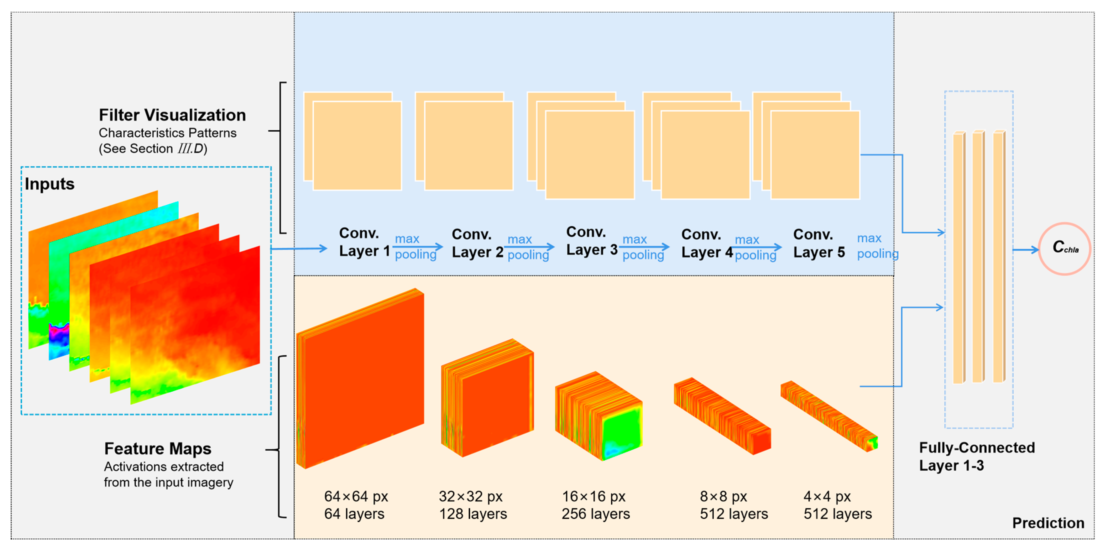
The Cchla-Net layer configurations were designed following the same principles of VGGNET16 [15], which has been demonstrated to be beneficial for the classification accuracy by increasing the depth with very small convolution filters. Figure 4 illustrates the network structure of Cchla-Net. The input to the Cchla-Net was a volume of a fixed size 64 × 64 × 6, and the output was the estimated Cchla normalized at the center pixel. Each pixel in the patch contained six normalized band ratio features. The Cchla-Net contained 13 convolution layers and three fully connected layers. The input volume was passed through a stack of convolution layers, where the filters used a small kernel size of 3 × 3 to capture the notion of left/right, up/down and center. The channel of convolution started from 64 in the first layer and then increased by a factor of 2, until it reached 512. The stride was fixed to 1 pixel, and the patch was padded with zeros to ensure the spatial size was preserved after the convolution. All convolution layers were equipped with a rectified linear unit function (ReLU) [17]. Spatial pooling was carried out by five max-pooling layers over a 2 × 2 window with stride of 2, following some of the convolution layers. The purpose of max-pooling layer was for downsampling and compressing features. The 3D volume was reshaped into a 1D vector by flattening and three fully connected layers: the first and second layer had 2048 neurons, respectively, and the final layer contained 1 neuron representing the normalized Cchla at the center pixel.
The stochastic gradient descent with momentum (SGDM) optimizer, which utilizes mini-batch stochastic gradient, was employed for optimization. The batch size was set to 128 and momentum to 0.9. To alleviate the overfitting, the L2 regularization was added to the loss function during the network’s backpropagation (the L2 penalty multiplier was set to 1.0 × 10⁻⁵), whereas the dropout regularization for the first two fully connected layers was adopted. The dropout ratio was set to 0.5, indicating that 50% of the neurons in the two fully connected layers were temporally retained when computing the loss function for the weights’ updating. In the training phase, the number of epochs was set to 30, and the initial learning rate was set to 0.01, with a drop factor of 0.1 after every 10 epochs. The half-mean-squared-error was used as the loss function, which is defined as:
where ti is the labeled sample, yi is the corresponding prediction and R is the number of samples.
4. Results and Discussion
4.1. MLR Adjustment
A total of 15 pairs of matchups from all campaigns were used for extracting coefficients of MLR adjustment and for the network testing independently. The MLR adjustment relied on in-situ measurements for reducing uncertainty and bias due to systematic perturbations, as resulting from absolute calibration and minimization of the atmospheric effects.
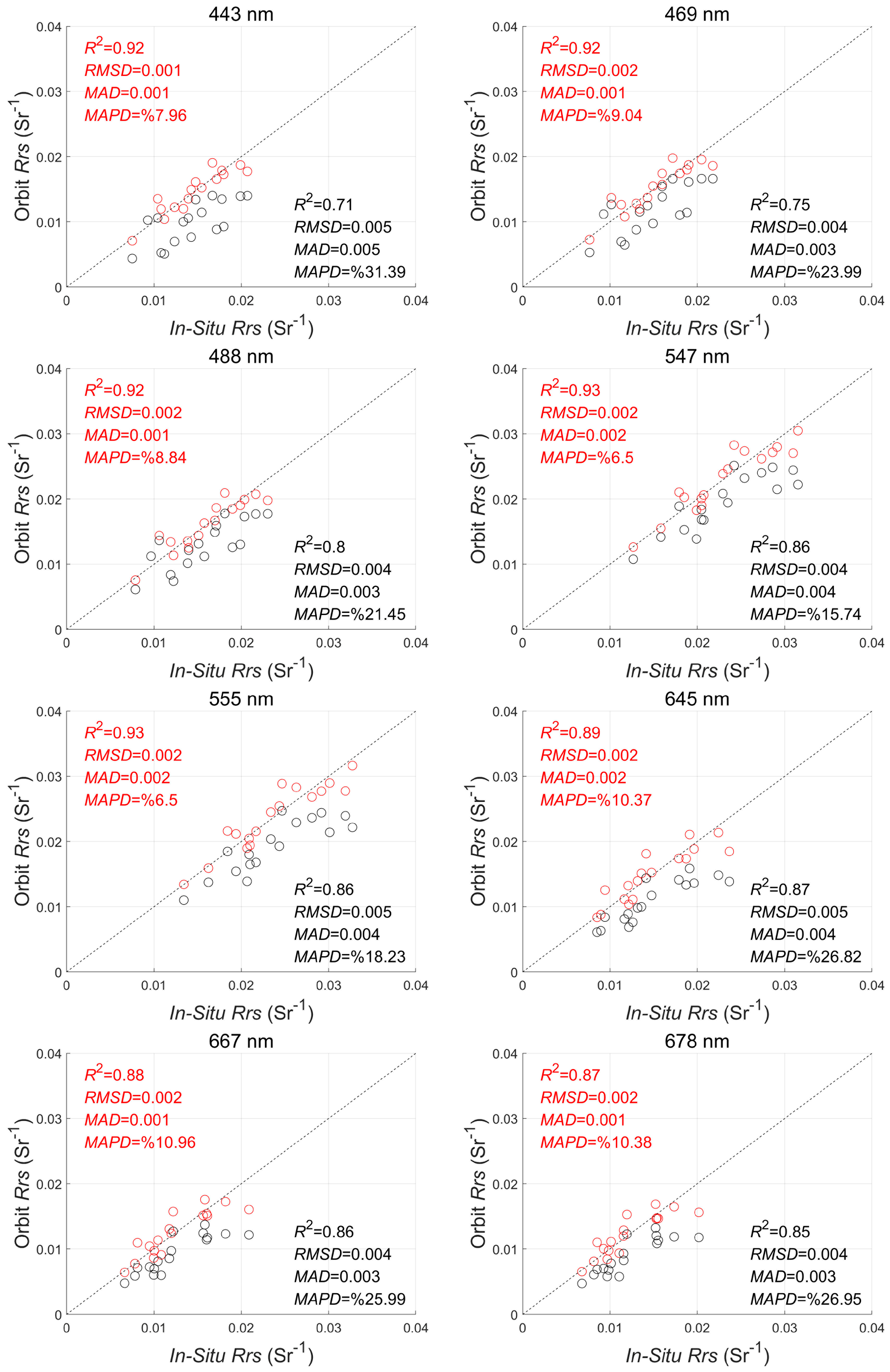
The scatterplots in Figure 5 showed the in-situ measurements versus the Rrs before (‘black’ plots) and after (‘red’ plots) adjustment at all visible bands. The approach appeared quite effective at those center wavelengths, with the largest differences between in-situ and orbit measurements, which were 443 and 469 nm, and other shorter wavelengths. As expected, a better performance after the adjustment was observed. Specifically, the RMSD and MAPD of MODIS derived Rrs, with respect to in-situ measured Rrs at 443 nm, had shown values of 0.005 Sr−1 and 31.4% before adjustment and a value of 0.001 Sr−1 and 7.3% after adjustment, respectively.
4.2. K-Fold Cross-Validation
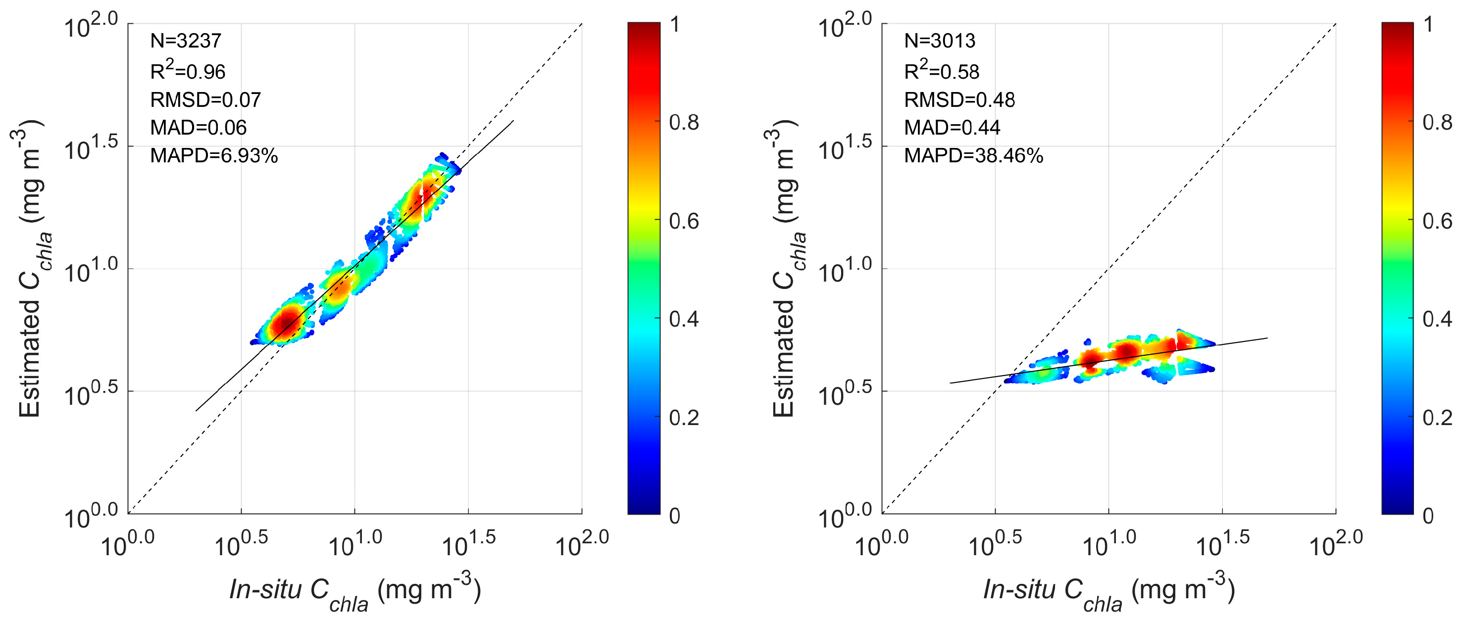
A 10-fold cross-validation was conducted, in which all patches and in-situ samples, except those for testing, were uniformly divided into 10 folds. In addition, a two-stage training consisting of pre-training and refinement was used. The first-stage procedure trained the network using the patches in which the Cchla was estimated by OC3M algorithm, whereas the second-stage procedure refined the network by utilizing the in-situ samples. The scatterplots of estimated versus original log10-transformed Cchla showed the network performance for cross-validation results (Figure 6).
The RMSD, MAD and MAPD of second-stage training were decreased compared to those of the first-training, with values that decreased from 0.48 to 0.07, 0.44 to 0.06 and 38.46% to 6.93%, respectively. The metrics of model accuracy were calculated in a log10-transformed scale. The pretrained network may have exhibited large discrepancy while applied to the validating dataset, implying that the first-stage training could not reach a global optimum, because the input Cchla was estimated by the OC3M algorithm, instead of from in-situ measurements. However, the purpose of first-stage training was to obtain suitable initial values of the network parameters. Training with the suitable initial values may have had a higher probability of obtaining a better generalized network, especially when the number of in-situ samples was insufficient.
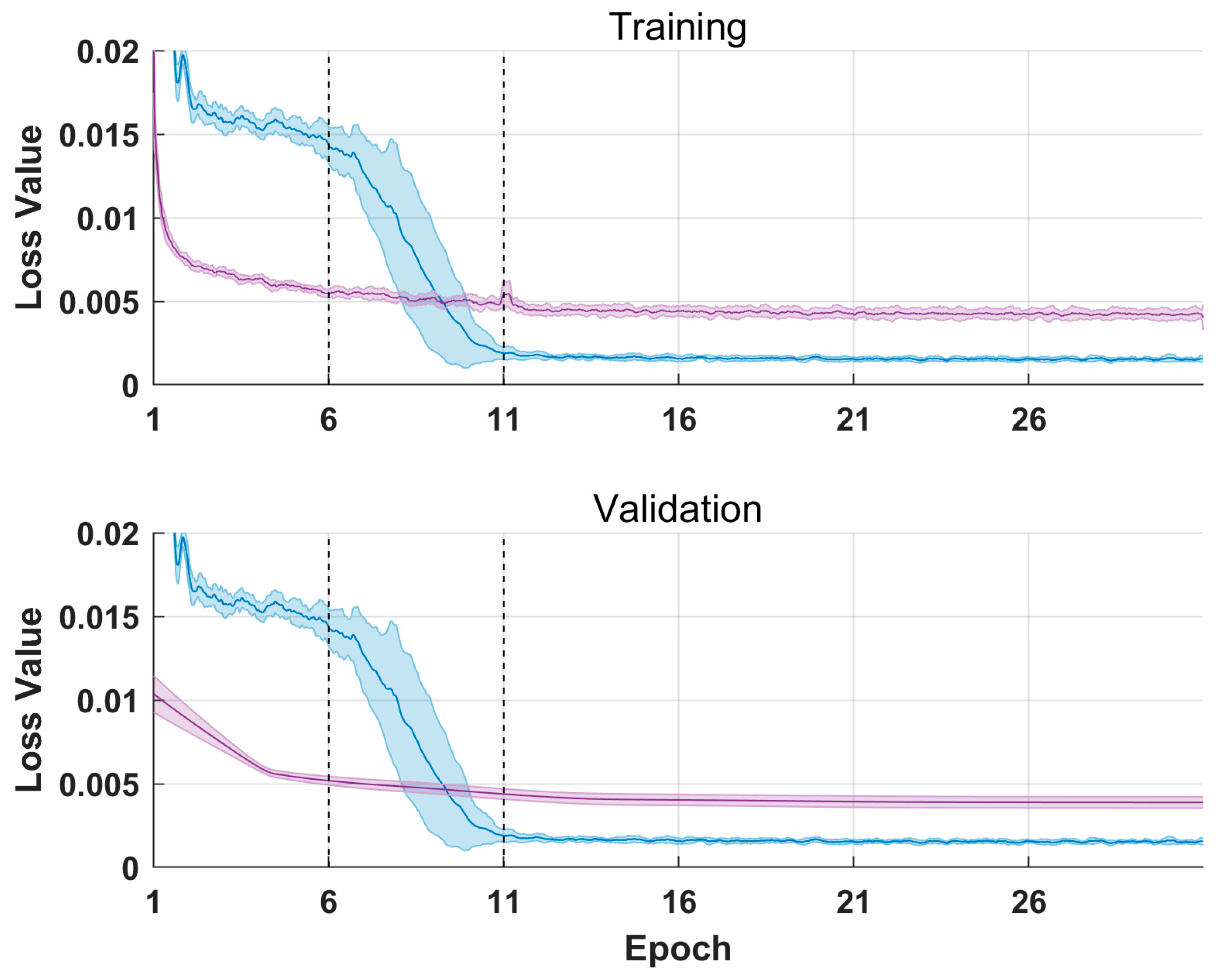
Convergence was evaluated by comparing the loss function of both one-stage and two-stage training. The loss function of 10-fold networks is presented in Figure 7, in which the upper panel shows the loss values in the training phase, and the lower panel shows the loss values in the validating phase. By using the refined parameters from one-stage training as the initial values of two-stage training, the network could converge more efficiently (about 6 epochs) than the one-stage training (about 11 epochs). Note that in both the training and validating phases, the final loss value of the one-stage network was smaller than that of the two-stage network, with values ranging between 0.004–0.007 and 0.004–0.005, respectively. It should be attributed to the different characteristics of the two datasets. The in-situ dataset was more discrete and contained less features than the imagery patches, despite it being oversampled by the SMOTE technique.
4.3. Model Performances
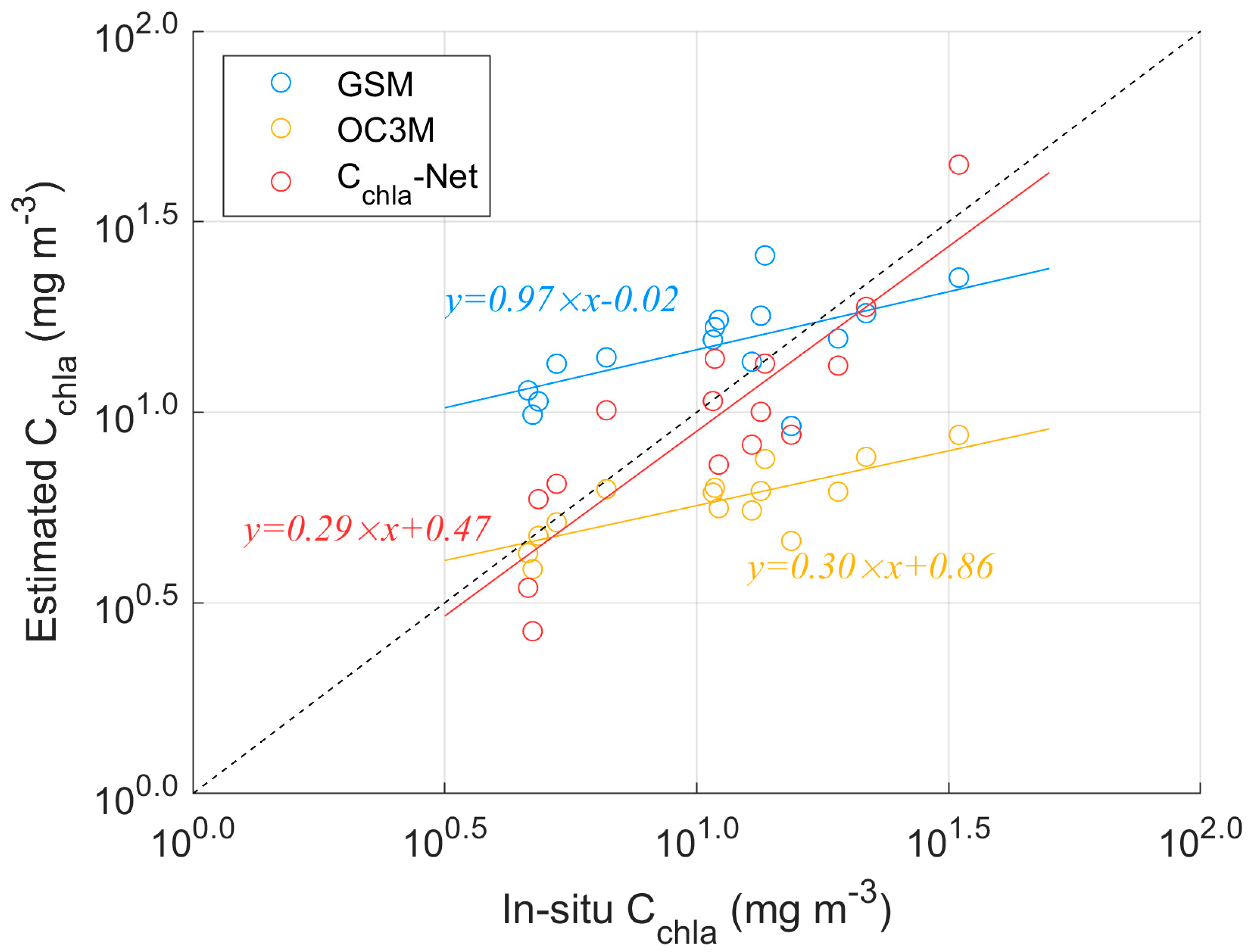
To evaluate the feasibility and performance, the proposed Cchla-Net approach was compared with two representative algorithms based on the independent testing dataset. The two algorithms were the OC3M, an empirical model, and the Garver-Siegel-Maritorena (GSM01), a semi-analytical model [10]. Statistics of the model performance are listed in Table 2. The Cchla-Net demonstrated a more satisfactory performance than the other two algorithms with higher R2, lower RMSD, lower MAD and lower MAPD, and its slope values of linear fit between estimated versus in-situ measured Cchla (0.97, closer to the 1:1 line) were higher than the other two models (0.29 and 0.30, Figure 8).
The OC3M model seemed to be underestimated in the high productive waters, especially when the Cchla was higher than 10 mg·m−3. The OC3 model was defined on the basis that the difference of two spectral reflectances was small, such that the absorption of suspended sediments and colored dissolved organic matter (CDOM) could be omitted. However, as typical Case-II waters, the optical properties of PRE waters were complex, and the total absorption of phytoplankton, suspended sediments and CDOM and the back-scattering coefficient of phytoplankton and suspended sediments were spectrally variant. Thus, the traditional band-ratio algorithms through blue and green ratios simply did not work for the high productive and turbid PRE waters. The GSM model showed a tendency to overestimate the lower Cchla. Meanwhile, the correlation between the GSM-estimated and in-situ measured Cchla was the lowest among the three algorithms (R2 = 0.63, lower than 0.77 and 0.85). The optimal GSM parameter values were hard to determine, due to the spareness of in-situ data on the backscattering coefficient of particulates bbp(λ) and the lack of predicted knowledge for the particle phase function [37]. The assumed constants of the model might not be appropriate for the PRE waters.
The estimated results of Cchla-Net were very close to the in-situ measurement, with its slope being around 1.0 and R2 being higher than 0.8. It demonstrated that the CNN model had a strong capability to learn the nonlinear relationship between the water-leaving Rrs and the corresponding Cchla of water body, as well as to make full use of the information at all the MODIS/Aqua’s visible bands. Additionally, the oversampling approach, the SMOTE technique, allowed us to provide a massive synthetic in-situ dataset for the second-stage training, and it turned out that the trained Cchla-Net generalized well to the independent testing dataset.
4.4. Model Applications
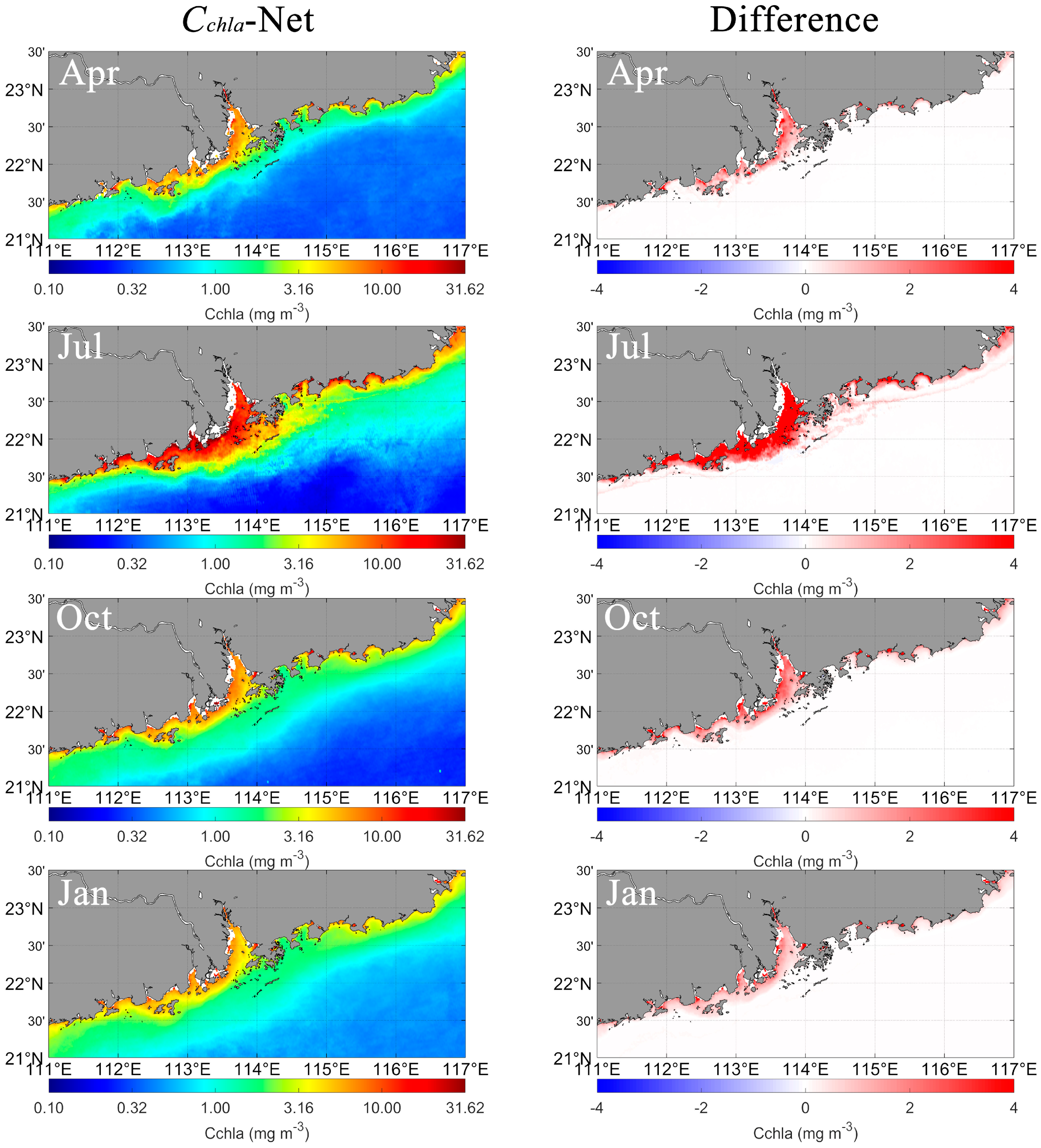
Given the satisfactory performance of the proposed Cchla-Net developed using in-situ dataset from PRE, this model was applied to all available MODIS/Aqua Cchla data between 2003 and 2020 to construct a multi-year product for PRE waters. Figure 9 showed the climatological monthly MODIS/Aqua Cchla estimated by Cchla-Net and the difference between Cchla-Net and OC3M models in the PRE. In general, the estimated Cchla from both models agreed well in the temporal patterns in the continental shelf. However, the difference between the two models in the coastal and estuarine areas was remarkable. Especially during summer, the maximal difference was up to 5.80 mg·m−3. Such differences were mainly due to the worse performance of OC3M model for high Cchla (>10 mg·m−3). Therefore, it is likely that Cchla-Net could serve as a better approach to provide the long-term MODIS/Aqua products than the classical OC3M model in the PRE waters. As expected, Cchla increased from the continental shelf to the coastal and estuarine area, as the latter received more direct influence of the highly productive freshwater. After exiting the LBPRE, the discharged freshwater generated a nearly stable bulge and formed a distinct plume, which was located in the southwestern LBPRE. The plume axis gradually shifted offshore as a result of the intensified Ekman drift. Therefore, The Cchla of western PRE was observed to be higher than that of eastern PRE. During summer, a tongue with a relatively higher Cchla tends to expand to the southern and southeastern LBPRE. Forced by the wind-driven coastal current, the plume was wider over the shelf due to the freshwater in the outer part of the bulge flowing downstream at the speed of the current. During winter, the plume was confined nearshore under the influence of the northeastly wind.
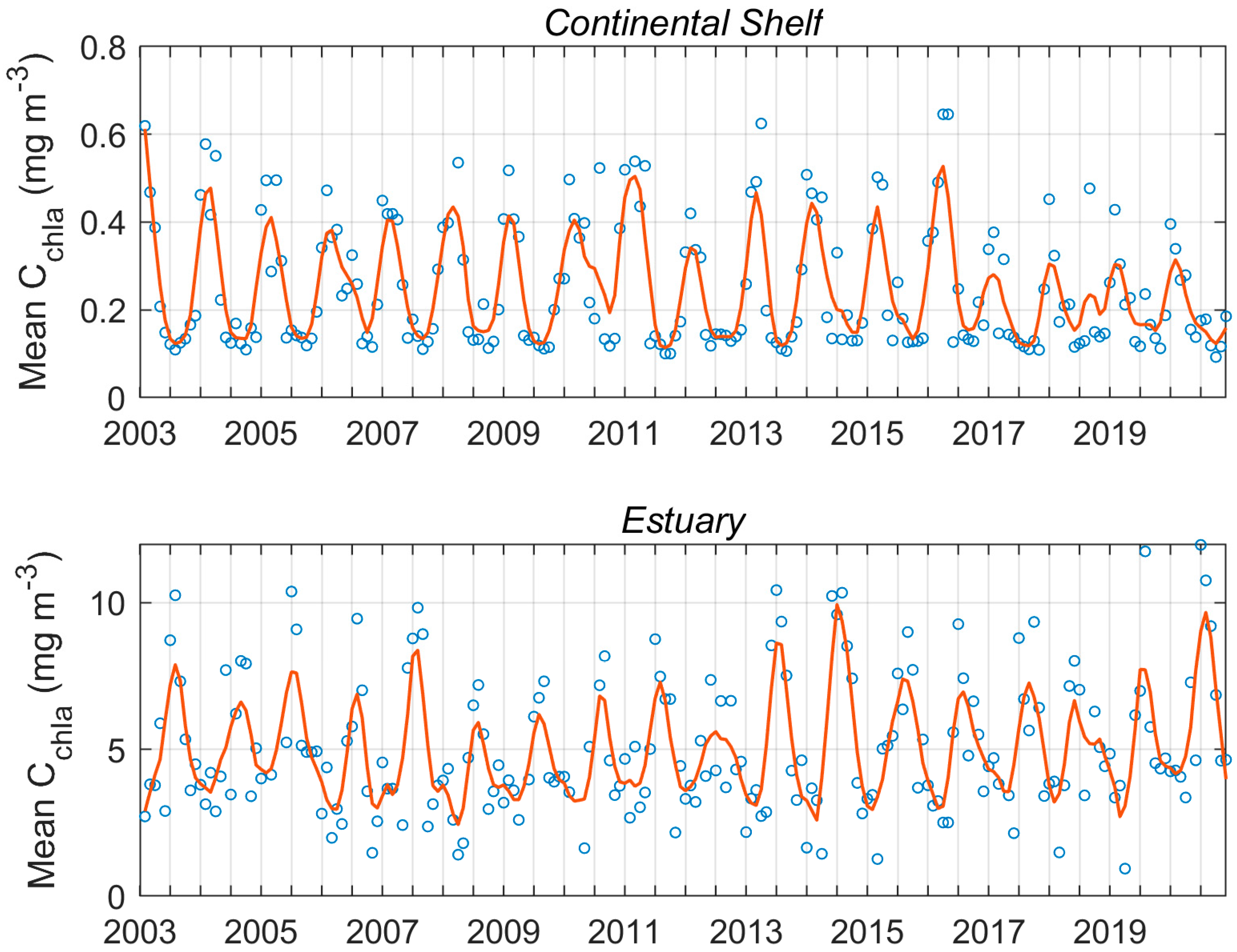
To facilitate quantitative interpretations, the spatial and seasonal variations in the coastal and estuarine area (‘Box 1’ in Figure 1), as well as the continental shelf (‘Box 2’ in Figure 1) were further examined. Figure 10 presents the monthly mean Cchla in both areas. The monthly mean values estimated by Cchla-Net ranged from 0.94 to 11.97 mg·m−3 in the LBPRE and from 0.09 to 0.65 mg·m−3 in the continental shelf. Different seasonal variations were found in coastal area and continental shelf, with relatively higher Cchla observed during summer in the former region and during winter in latter region. These seasonal variations appeared to be regulated primarily by river discharge and mixing of the upper ocean [23].
5. Conclusions
This study found that the Cchla-Net showed an apparent advantage over the empirical and semi-analytical models for extremely high Cchla. Therefore, Cchla-Net might be a promising method for the Cchla retrieval in optically complex coastal and estuarine waters. The proposed Cchla-Net model worked well for low to high values especially, while the OC3M algorithm tended to underestimate high values in the coastal and estuarine area. The MLR adjustment, which specifically relies on matchups of corresponding in-situ and orbit-measured Rrs to capture systematic differences, could remove the difference likely due to uncertainties in the absolute calibration of sensors and the minimization of atmospheric perturbations. The novel adaptive synthetic oversampling technique improved the DL model with respect to the distribution of dataset in two ways: (i) reducing the bias introduced by the imbalanced distribution of the dataset; (ii) adaptively shifting the classification decision boundary to be more focused on the difficult to learn samples.
Considering the high performance, it has a great potential to be applied in the PRE, especially for the productive and optically complex coastal and estuarine waters. However, there is still room for improvement. As a data-driven method, input training the dataset directly impacts the network performance. The accuracy of the DL network largely depends on the in-situ dataset, which covered a wide range of Cchla variations. More in-situ datasets are required to improve the model applicability. Furthermore, the OC3M products were used on a global scale and could not be directly applied to the PRE waters. Collecting more in-situ samples to adjust the parameters of the OC3M model could also be beneficial for the DL network training.
Author Contributions
Writing—original draft preparation, H.Y.; Project Administration, S.T.; Methodology, C.Y. All authors have read and agreed to the published version of the manuscript.
Funding
This research was supported by Hainan Key Research and Development Program (No. ZDYF2020174), the Key Special Project for Introduced Talents Team of Southern Marine Science and Engineering Guangdong Laboratory (Guangzhou) (GML2019ZD0302), the Guangdong Special Support Program (2019BT02H594), the State Key Laboratory of Tropical Oceanography Independent Research Fund (Grant no. LTOZZ2103) and the Research & Development Projects in Key Areas of Guangdong Province, China (No. 2020B1111020004).
Institutional Review Board Statement
Not applicable.
Informed Consent Statement
Not applicable.
Data Availability Statement
The MODIS data are available at the National Aeronautics and Space Agency (NASA) ocean color data archive (https://oceancolor.gsfc.nasa.gov) (accessed on 14 September 2021).
Acknowledgments
The authors would like to thank the NASA Goddard Space Center for providing MODIS data and the NASA OBPG group for providing the SeaDAS software package. The colleagues in the Ocean Color group of the South China Sea Institute of Oceanology, Chinese Academy of Sciences, are greatly appreciated for their effort in collecting and processing the samples. The numerical analysis was supported by the High Performance Computing Division in the South China Sea Institute of Oceanology.
Conflicts of Interest
The authors declare no conflict of interest.
References
- Chen, C.; Shi, P.; Larson, M.; Jonsson, L. Estimation of chlorophyll-a concentration in the Zhujiang estuary from SeaWiFS data. Acta Oceanol. Sin. 2002, 21, 55–65. [Google Scholar]
- Zheng, G.; DiGiacomo, P.M. Uncertainties and applications of satellite-derived coastal water quality products. Prog. Oceanogr. 2017, 159, 45–72. [Google Scholar] [CrossRef]
- Son, Y.; Kim, H. Empirical ocean color algorithms and bio-optical properties of the western coastal waters of Svallbard Arctic. ISPRS J. Photogram. Remote Sens. 2018, 139, 272–283. [Google Scholar] [CrossRef]
- Reilly, J.E.O. SeaWiFS Postlaunch Calibration and Validation Analyses, Part 3. In NASA Technical Memorandum; Hooker, S.B., Firestone, E.R., Eds.; NASA Goddard Space Flight Center: Greenbelt, MD, USA, 2000; Volume 11, p. 49. [Google Scholar]
- Morel, A.; Prieur, L. Analysis of variations in ocean color. Limnol. Oceanogr. 1977, 22, 709–722. [Google Scholar] [CrossRef]
- Gordon, H.R.; Morel, A. Remote Assessment of Ocean Color for Interpretation of Satellite Visible Imagery, A Review; Springer: New York, NY, USA, 1983; Volume 4. [Google Scholar]
- O’Reilly, J.E.; Maritorena, S.; Mitchell, B.G.; Siegel, D.A.; Carder, K.L.; Garver, S.A.; Kahru, M.; McClain, C. Ocean color chlorophyll algorithms for SeaWiFS. J. Geophys. Res. 1998, 103, 24937–24953. [Google Scholar] [CrossRef] [Green Version]
- Garver, S.A.; Siegel, D.A. Inherent optical property inversion of ocean color spectra and its biogeochemical interpretation. I. Time series from the Sargasso Sea. J. Geophys. Res. 1997, 102, 18607–18625. [Google Scholar] [CrossRef]
- Lee, Z.; Carder, K.L.; Arnone, R.A. Deriving inherent optical properties from water color: A multiband quasi-analytical algorithm for optically deep waters. Appl. Opt. 2002, 41, 5755–5772. [Google Scholar] [CrossRef] [PubMed]
- Maritorena, S.; Siegel, D.A.; Peterson, A.R. Optimization of a semianalytical ocean color model for global-scale applications. Appl. Opt. 2002, 41, 2705–2714. [Google Scholar] [CrossRef]
- Kampel, M.; Frouin, J.R.; Gaeta, A.S.; Lorenzzetti, J.A.; Pompeu, M. Satellite estimates of chlorophyll-a concentration in the Brazilian Southeastern continental shelf and slope waters, Southwestern Atlantic. In Coastal Ocean Remote Sensing; International Society for Optics and Photonics: Bellingham, WA, USA, 2007; Volume 6680. [Google Scholar]
- Srivastava, A.; Sahoo, B.; Raghuwanshi, N.S.; Singh, R. Evaluation of variable-infiltration capacity model and MODIS-terra satellite-derived grid-scale evapotranspiration estimates in a River Basin with Tropical Monsoon-Type climatology. J. Irrig. Drain. Eng. 2017, 143, 04017028. [Google Scholar] [CrossRef] [Green Version]
- Elbeltagi, A.; Kumari, N.; Dharpure, J.K.; Mokhtar, A.; Alsafadi, K.; Kumar, M.; Kuriqi, A. Prediction of combined terrestrial evapotranspiration index (CTEI) over large river basin based on machine learning approaches. Water 2021, 13, 547. [Google Scholar] [CrossRef]
- Liu, H.Z.; Li, Q.Q.; Bai, Y.; Yang, C.; Wang, J.J.; Zhou, Q.M.; Hu, S.B.; Shi, T.Z.; Liao, X.M.; Wu, G.F. Improving satellite retrieval of oceanic particulate organic carbon concentrations using machine learning methods. Remote Sens. Environ. 2021, 256, 112316. [Google Scholar] [CrossRef]
- Zhang, L.; Zhang, L.; Du, B. Deep learning for remote sensing data: A technical tutorial on the state of the art. IEEE Geosci. Remote Sens. Mag. 2016, 4, 22–40. [Google Scholar] [CrossRef]
- Zhu, X.X.; Tuia, D.; Mou, L.; Xia, G.S.; Zhang, L.; Xu, F.; Fraundorfer, F. Deep learning in remote sensing: A comprehensive review and list of resources. IEEE Geosci. Remote Sens. Mag. 2017, 5, 8–36. [Google Scholar] [CrossRef] [Green Version]
- Krizhevsky, A.; Sutskever, I.; Hinton, G. ImageNet Classification with Deep Convolutional Neural Networks. In Proceedings of the 25th International Conference on Neural Information Processing Systems NIPS, Lake Taho, NV, USA, 3–6 December 2012; Curran Associates Inc.: Red Hook, NY, USA, 2012; Volume 25. [Google Scholar]
- Simonyan, K.; Zisserman, A. Very Deep Convolutional Networks for Large-scale Image Recognition. In Proceedings of the 3rd International Conference on Learning Representations, ICLR, San Diego, CA, USA, 7–9 May 2015. [Google Scholar]
- He, K.; Zhang, X.; Ren, S.; Sun, J. Deep residual learning for image recognition. In Proceedings of the IEEE International Conference Computer Vision and Pattern Recognition (CVPR), Las Vegas, NV, USA, 27–30 June 2016; pp. 770–778. [Google Scholar]
- Girshick, R.; Donahue, J.; Darrell, T.; Malik, J. Region-based convolutional networks for accurate object detection and semantic segmentation. IEEE Trans. Pattern Anal. Mach. Intell. 2016, 38, 142–158. [Google Scholar] [CrossRef]
- Redmon, J.; Divvala, S.; Girshick, R.; Farhadi, A. You only look once: Unified, real-time object detection. In Proceedings of the IEEE International Conference Computer Vision and Pattern Recognition (CVPR), Las Vegas, NV, USA, 27–30 June 2016; pp. 779–788. [Google Scholar]
- Nazeer, M.; Nichol, J.E. Development and application of a remote sensing-based Chlorophyll-a concentration prediction model for complex coastal waters of Hong Kong. J. Hydrol. 2016, 532, 80–89. [Google Scholar] [CrossRef]
- Ye, H.B.; Yang, C.Y.; Tang, S.L.; Chen, C.Q. The phytoplankton variability in the Pearl River estuary based on VIIRS imagery. Cont. Shelf Res. 2020, 207, 104228. [Google Scholar] [CrossRef]
- Gan, J.P.; Li, H.; Curchitser, E.N.; Haidvogel, D.B. Modeling South China Sea circulation: Response to seasonal forcing regimes. J. Geophys. Res. 2006, 111, C06034. [Google Scholar] [CrossRef]
- Xie, S.P.; Xie, Q.; Wang, D.X.; Liu, W.T. Summer upwelling in the South China Sea and its role in regional climate variations. J. Geophys. Res. 2003, 108, 3261. [Google Scholar] [CrossRef] [Green Version]
- Yang, C.Y.; Ye, H.B.; Tang, S.L. Seasonal variability of diffuse attenuation coefficient in the Pearl River Estuary from Long-Term Remote Sensing Imagery. Remote Sens. 2020, 12, 2269. [Google Scholar] [CrossRef]
- Li, M.G.; Yan, Y.; Han, X.J.; Li, W.D. Physical model study for effects of the HongKong-Zhuhai-Macao Bridge on harbors and channels in Lingdingyang Bay of the Pearl River Estuary. Ocean Coast. Manag. 2019, 177, 76–86. [Google Scholar]
- Chen, C.; Tang, S.; Pan, Z.; Zhan, H.; Larson, M.; Jonsson, L. Remotely sensed assessment of water quality levels in the Pearl River Estuary, China. Mar. Pollut. Bull. 2007, 54, 1267–1272. [Google Scholar] [CrossRef] [PubMed]
- Zhao, J.; Cao, W.; Wang, G.; Yang, D.; Yang, Y.; Sun, Z.; Zhou, W.; Liang, S. The variations in optical properties of CDOM throughout an algal bloom event. Estuar. Coast. Shelf Sci. 2009, 82, 225–232. [Google Scholar] [CrossRef]
- Mueller, J.L. Radiometric Measurements and Data Analysis Protocols; Goddard Space Flight Center: Greenbelt, MD, USA, 2003.
- Welschmeyer, N. Fluorometric analysis of chlorophyll a in the presence of chlorophyll b and pheopigments. Limnol. Oceanogr. 1994, 38, 1985–1992. [Google Scholar] [CrossRef]
- Ruddick, K.G.; Ovidio, F.; Rijkeboer, M. Atmospheric correction of SeaWiFS imagery for turbid coastal and inland waters. Appl. Opt. 2000, 39, 897–912. [Google Scholar] [CrossRef] [Green Version]
- Evers-King, H.; Martinez-Vicente, V.; Brewin, R.J.W.; Dall’Olmo, G.; Hickman, A.E.; Jackson, T.; Kostadinov, T.S.; Krasemann, H.; Loisel, H.; Röttgers, R.; et al. Validation and Intercomparison of ocean color algorithms for estimating particulate organic carbon in the oceans. Front. Mar. Sci. 2017, 4, 251. [Google Scholar] [CrossRef]
- D’Alimonte, D.; Zibordi, G.; Melin, F. A statistical method for generating Cross-Mission consistent normalized water-leaving radiances. IEEE Trans. Geosci. Remote Sens. 2008, 46, 4075–4093. [Google Scholar] [CrossRef]
- Chawla, N.V.; Bowyer, K.W.; Hall, L.O.; Kegelmeyer, W.P. SMOTE: Synthetic minority over-sampling technique. J. Artif. Intell. Res. 2002, 16, 321–357. [Google Scholar] [CrossRef]
- He, H.; Bai, Y.; Garcia, E.A.; Li, S. ADASYN: Adaptive synthetic sampling approach for imbalanced learning. In Proceedings of the IEEE International Joint Conference on Neural Networks, Hong Kong, China, 1–8 June 2008; pp. 1322–1328. [Google Scholar]
- Morel, A.; Maritorena, S. Bio-optical properties of oceanic waters: A reappraisal. J. Geophys. Res. 2001, 106, 7163–7180. [Google Scholar] [CrossRef] [Green Version]
Figure 1.
Study area, location of the sampling stations and in-situ measured Rrs.

Figure 2.
Overall framework of model development and application.

Figure 3.
R2 from linear regressions between different band ratios and the Cchla based on the in-situ dataset. The x axis shows the wavelength at which Rrs was used as denominator and the y axis for the wavelengths at which Rrs was used as numerator.
Figure 3.
R2 from linear regressions between different band ratios and the Cchla based on the in-situ dataset. The x axis shows the wavelength at which Rrs was used as denominator and the y axis for the wavelengths at which Rrs was used as numerator.

Figure 4.
Network structure of Cchla-Net.

Figure 5.
Scatterplots of the in-situ Rrs versus the original and adjusted MODIS/Aqua Rrs at MODIS\Aqua’s visible bands (plots at 412 nm were not given, because the Rrs at this band was not used in the network. Black cirles: original Rrs; Red circles: adjusted Rrs).
Figure 5.
Scatterplots of the in-situ Rrs versus the original and adjusted MODIS/Aqua Rrs at MODIS\Aqua’s visible bands (plots at 412 nm were not given, because the Rrs at this band was not used in the network. Black cirles: original Rrs; Red circles: adjusted Rrs).

Figure 6.
Scatterplots of estimated versus original (synthetic dataset) Cchla for two-stage training (left) and only first-stage training (right).
Figure 6.
Scatterplots of estimated versus original (synthetic dataset) Cchla for two-stage training (left) and only first-stage training (right).

Figure 7.
Comparison of model convergence. The curves represent the loss values at each epoch during the training and validating phases (‘red’ plots denote the two-stage values, and ‘blue’ plots denote the one-stage values).
Figure 7.
Comparison of model convergence. The curves represent the loss values at each epoch during the training and validating phases (‘red’ plots denote the two-stage values, and ‘blue’ plots denote the one-stage values).

Figure 8.
Scatterplots of model-estimated and in-situ measured Cchla.

Figure 9.
Climatological monthly MODIS/Aqua Cchla between 2003 and 2020, estimated by Cchla-Net, OC3M and the difference of both models. Four months (April, July, October and January) were chosen, representing four seasons (spring, summer, autumn and winter).
Figure 9.
Climatological monthly MODIS/Aqua Cchla between 2003 and 2020, estimated by Cchla-Net, OC3M and the difference of both models. Four months (April, July, October and January) were chosen, representing four seasons (spring, summer, autumn and winter).

Figure 10.
Time series of monthly mean Cchla derived from MODIS/Aqua measurements using the Cchla-Net in the estuary and continental shelf.
Figure 10.
Time series of monthly mean Cchla derived from MODIS/Aqua measurements using the Cchla-Net in the estuary and continental shelf.


Table 1.
Summary of in-situ campaigns during 2003 and 2012.
| No. | Date | N | Range of Cchla (mg·m−3) |
|---|---|---|---|
| 1 | 6 January 2003 | 18 | 7.82 ± 10.79 |
| 2 | 6 January 2004 | 18 | 14.48 ± 11.45 |
| 3 | 18 May 2004 | 17 | 15.17 ± 13.03 |
| 4 | 15 August 2009 | 16 | 6.10 ± 4.65 |
| 5 | 22 October 2009 | 16 | 5.55 ± 4.85 |
| 6 | 22 November 2009 | 16 | 2.43 ± 1.83 |
| 7 | 13 December 2009 | 16 | 4.40 ± 1.51 |
| 8 | 1 February 2010 | 16 | 3.24 ± 1.38 |
| 9 | 4 July 2010 | 16 | 13.73 ± 6.29 |
| 10 | 5 June 2012 | 16 | 3.77 ± 2.02 |
Table 2.
Statistical descriptions of three different model’s performance; the best metric is in bold.
Table 2.
Statistical descriptions of three different model’s performance; the best metric is in bold.
| R2 | RMSD | MAD | MAPD (%) | |
|---|---|---|---|---|
| Cchla-Net | 0.85 | 0.15 | 0.13 | 14.34 |
| GSM | 0.63 | 0.25 | 0.22 | 25.61 |
| OC3M | 0.77 | 0.32 | 0.26 | 22.54 |
Publisher’s Note: MDPI stays neutral with regard to jurisdictional claims in published maps and institutional affiliations. |
© 2021 by the authors. Licensee MDPI, Basel, Switzerland. This article is an open access article distributed under the terms and conditions of the Creative Commons Attribution (CC BY) license (https://creativecommons.org/licenses/by/4.0/).
Share and Cite
MDPI and ACS Style
Ye, H.; Tang, S.; Yang, C. Deep Learning for Chlorophyll-a Concentration Retrieval: A Case Study for the Pearl River Estuary. Remote Sens. 2021, 13, 3717. https://0-doi-org.brum.beds.ac.uk/10.3390/rs13183717
AMA Style
Ye H, Tang S, Yang C. Deep Learning for Chlorophyll-a Concentration Retrieval: A Case Study for the Pearl River Estuary. Remote Sensing. 2021; 13(18):3717. https://0-doi-org.brum.beds.ac.uk/10.3390/rs13183717
Chicago/Turabian StyleYe, Haibin, Shilin Tang, and Chaoyu Yang. 2021. "Deep Learning for Chlorophyll-a Concentration Retrieval: A Case Study for the Pearl River Estuary" Remote Sensing 13, no. 18: 3717. https://0-doi-org.brum.beds.ac.uk/10.3390/rs13183717
Note that from the first issue of 2016, this journal uses article numbers instead of page numbers. See further details here.