
The Role of Satellite InSAR for Landslide Forecasting: Limitations and Openings


1
Department of Earth Sciences & CERI Research Center on Geological Risks, Sapienza University of Rome, P. le A. Moro 5, 00185 Rome, Italy
2
NHAZCA S.r.l. Startup, Sapienza University of Rome, via V. Bachelet 12, 00185 Rome, Italy
*
Author to whom correspondence should be addressed.
Remote Sens. 2021, 13(18), 3735; https://0-doi-org.brum.beds.ac.uk/10.3390/rs13183735
Submission received: 19 July 2021
/
Revised: 6 September 2021
/
Accepted: 13 September 2021
/
Published: 17 September 2021
(This article belongs to the Special Issue SAR Imagery for Landslide Detection and Prediction)
Abstract
:The paper explores the potential of the satellite advanced differential synthetic aperture radar interferometry (A-DInSAR) technique for the identification of impending slope failure. The advantages and limitations of satellite InSAR in monitoring pre-failure landslide behaviour are addressed in five different case histories back-analysed using data acquired by different satellite missions: Montescaglioso landslide (2013, Italy), Scillato landslide (2015, Italy), Bingham Canyon Mine landslide (2013, UT, USA), Big Sur landslide (2017, CA, USA) and Xinmo landslide (2017, China). This paper aimed at providing a contribution to improve the knowledge within the subject area of landslide forecasting using monitoring data, in particular exploring the suitability of satellite InSAR for spatial and temporal prediction of large landslides. The study confirmed that satellite InSAR can be successful in the early detection of slopes prone to collapse; its limitations due to phase aliasing and low sampling frequency are also underlined. According to the results, we propose a novel landslide predictability classification discerning five different levels of predictability by satellite InSAR. Finally, the big step forward made for landslide forecasting applications since the beginning of the first SAR systems (ERS and Envisat) is shown, highlighting that future perspectives are encouraging thanks to the expected improvement of upcoming satellite missions that could highly increase the capability to monitor landslides’ pre-failure behaviour.
1. Introduction
The availability of SAR satellite images since 1992 has allowed the development of A-DInSAR (advanced differential synthetic aperture radar interferometry) processing methods since the early 2000s [1,2,3]. The main factors that contributed to the spread and development of satellite SAR interferometry can be summarized as follows: The launch of several satellite missions belonging to different national and international space agencies, the improvement of satellite mission technologies, the enhancement of computing capabilities and the improvement of processing algorithms. Nowadays, satellite SAR interferometry is considered an effective technique for land, structure and infrastructure monitoring, finding several applications in landslide risk mitigation strategies at different stages and scales [4,5,6,7,8,9,10,11,12,13,14,15,16,17,18,19,20,21,22,23,24].
The increasing availability of SAR satellite images (in terms of both spatial and temporal coverage) and the development of accurate processing algorithms [1,3,25,26,27,28,29] led to the opportunity to use satellite technologies for continuous monitoring applications, allowing to reflect on the possibility to exploit the satellite InSAR technique for landslides forecasting purposes. In A-DInSAR approaches, several tens of SAR images collected over time over the same area with the same acquisition geometry (interferometric stack) are used to overcome the main limitations due to the atmospheric phase screen (APS) and residual topography [1,2,26]. Persistent Scatterers Interferometry (PSI) is one of the first and most used A-DInSAR techniques, based on the analysis of specific targets on the Earth’s surface (called Persistent Scatterers, PSs) characterized by long time-coherent behaviour, allowing to retrieve: (i) The deformational trend during the investigated time period with millimetre accuracy; (ii) the time series of displacement; (iii) the residual height with respect to the reference DEM (Digital Elevation Model) used.
In this paper the role of satellite SAR interferometry for landslide forecasting is evaluated, giving an overview of some cases already presented in the scientific literature and new insights. Specifically, according to the creep theory [30,31], the potential of satellite InSAR to monitor precursor phenomena of large landslides and their spatial and temporal predictability, also in terms of Time of Failure estimation (ToF, [32,33,34,35]) is revised.
The first studies published on this topic regard the theoretical assessments on the possibility to exploit satellite InSAR to monitor a landslide process during the pre-failure stage [36,37,38,39,40]. The preliminary evaluation carried out by Mazzanti et al. (2011) on “landslides forecasting analysis by displacement time series derived from satellite InSAR data” highlights the limitations that must be accounted for, such as: The availability of data, radar distortions, the presence of backscatters, the moving direction of the landslide, the extension of landslides and the magnitude of precursory phenomena (i.e., the length of the tertiary creep phase and the rate of deformations). The first basic consideration is that several landslide processes cannot be investigated using the satellite InSAR technique.
Assuming the presence of a coherent target in correspondence with a landslide area is satisfied, Moretto et al. 2017 [40] performed a first quantitative analysis concerning the “Assessment of Landslide Pre-Failure Monitoring and Forecasting Using Satellite SAR Interferometry”, considering two major limitations of the technique to monitor the pre-failure behaviour: (i) The revisit time (i.e., the sampling period of the data acquisition) and (ii) the phase ambiguity constraints. The acquisition of slope deformations before the collapse was simulated for 58 landslides, considering the features of satellite missions of the past, present and future. From the study, it was found that 30% of the landslide events collected could have been monitored during the acceleration phase considering the current features of Sentinel-1 constellation.
In recent years, taking advantage of the increasing temporal and spatial resolutions of new SAR satellite missions (Sentinel-1 and COSMO-SkyMed in particular), several retrospective analyses of past landslides have been carried out using A-DInSAR methods, retrieving the deformational behaviour during the pre-failure stage [39,40,41,42,43,44,45,46]. In particular, the Xinmo landslide (24 June 2017; China) gained great attention in the satellite remote sensing community. It was the first landslide where clear precursors were observed with the satellite InSAR technique with time series of displacement showing the typical deformational behaviour of the tertiary creep phase [39,41].
In this paper we describe five different retrospective analyses carried out on natural and man-made slopes in different environments and with different InSAR sensors (Figure 1):
- (1)
- Montescaglioso landslide (3 December 2013; Italy), using COSMO-SkyMed imagery in the time period between May 2011 and December 2013;
- (2)
- Scillato landslide (10 April 2015; Italy), using COSMO-SkyMed imagery in the time period between January 2013 and March 2015 (Moretto et al., 2018);
- (3)
- Bingham Canyon Mine landslide (10 April 2013), using the RADARSAT-2 dataset collected between December 2008 and March 2013;
- (4)
- Muddy Creek landslide (25 May 2017; CA, USA), using Sentinel-1 dataset acquired in the period May 2015–May 2017;
- (5)
- Xinmo landslide (24 June 2017; China), using Sentinel-1 imagery acquired between October 2014 and June 2017.
The results obtained using the A-DInSAR technique were analysed and exploited for forecasting purposes. A Time Series Analysis (TSA) was performed according to the following approaches:
- A Trend Change Detection Analysis (TCDA) was performed in order to detect trend changes in the time series of displacement, which can be associated to critical phases in a landslide’s life cycle;
- landslide forecasting methods were applied using A-DInSAR time series of displacement for the time of failure estimation.
Finally, the study allowed to propose a new classification regarding the predictability of large landslides from satellite InSAR, discussing, among the predictability versus unpredictability of landslides, the spatial and temporal prediction opportunity offered by present satellite missions and future perspectives.
2. Materials and Methods
The study workflow is presented in Figure 2. The A-DInSAR retrospective analyses were carried out for the five case histories. Time series of displacement was analysed (TSA) to assess and classify the deformational behaviour of the landslides during the pre-failure stage. First, the TCDA was applied, followed by a full time of failure analysis in case of trend change identification.
Results obtained with landslide forecasting methods were analysed to understand the reliability of prediction, focusing on the occurrence of spatial and/or temporal clusters in predictions. For all the landslides, the results were assessed and interpreted globally (including InSAR and TSA results, correlation with rainfall data, interferograms, etc.) allowing to retrieve interesting information regarding the landslide pre-failure behaviour.
2.1. Landslide Forecasting Methods
The scientific community started to explore landslide behaviour during the first half of the twentieth century [30]. In 1950, Terzaghi recognized the relation between landslide evolution and creep theory; he was the first to connect the progressive deformation process affecting a slope before failure with the creep theory, laying the foundations for landslide prediction.
The creep theory describes the plastic deformation of materials exposed to a constant stress below their yield stress. Within engineering geology and material science, creep theory describes the deformation of the slope under constant shear stress till failure, thus representing the time-dependent deformational behaviour of a slope towards failure.
Continuous deformation, which progresses under constant stress, is a material behaviour of evident interest to a wide spectrum of scientists. If deformation is likely to accelerate towards failure, understanding and modelling the process becomes crucial “to estimating the useful life of machines and structures, to anticipating the behaviour of artificial embankments and natural and cut slopes, and to evaluating the hazards their possible failure presents to property and people” [31].
Over many years, a big number of scientific studies were carried out, producing a very large literature [30,31,32,33,34,35].
In 1982, Varnes [31] presented and described the progressive failure of materials under constant stress, using a deformational model composed by three different stages: The primary, secondary and tertiary creep. The tertiary creep phase represents the fundamental phase for the application of landslide forecasting methods (or semi-empirical methods) [47,48,49,50,51,52,53,54,55]. One of the most known, used and powerful methods is the Inverse Velocity method (INV), developed by Fukuzono (1985, [32]) and subsequently improved by Voight (1988, [34]) and Cornelius and Voight (1995, [35]).
Analysing the rate of precursory phenomena for volcanic eruptions, Voight (1988) wrote the following equation:
where is the acceleration, is the velocity, A and α are semi-empirical constants. The author suggested that several parameters could be used in the relation (e.g., strain, rotation, translation or seismic-energy release), thus including any kind of precursor phenomena which can be measured in terms of velocity and acceleration. Based on equation 1, different failure forecasting methods were proposed [35]. In this study, we make use of the following two forecasting methods:
- The non-linear fitting technique (NL Technique, Figure 3b, [35,38]), consisting in the non-linear data approximation using the least-squares approach. A and α constants are found iteratively by minimizing the error between the real pre-failure monitoring data and the given function. ToF is computed assuming that, when the strain rate tends to infinity, the slope tends to failure; thus, it matches with the curve’s asymptote. The NL method can be applied only for α > 1.
2.2. Satellite A-DInSAR
The observation of the accelerative behaviour preceding a slope before failure is fundamental for temporal prediction and for the application of forecasting methods. The basic requirement for the application of landslide forecasting methods is the monitoring of deformations affecting a slope before the failure.
Satellite A-DInSAR is a powerful radar-based remote sensing technique that allows to measure displacements of the ground and structures over time, reaching millimetre-level accuracy, for those measurement points characterized by a high stability of the backscattered radar signal (i.e., coherent targets). It is a multi-image processing technique able to provide the time series of displacement for both wide areas (thousands of square kilometres) and small areas (i.e., single slope or structure).
The analyses carried out in this study are based on the exploitation of the PSI (persistent scatterers interferometry) techniques ([1,2,26]). The PSI approach is based on the observation that “man-made features remained coherent in radar interferograms over long time spans, while their surrounding was completely decorrelated” [26]. Persistent scatterers interferometry allows to reduce the temporal and geometrical decorrelation issues and the atmospheric artefacts by analysing the interferometric phase of individual long time-coherent scatterers in a stack of many tens of differential interferograms (i.e., pixels/scatterers that are coherent in all the interferograms). The peculiarity of the PSI technique is the use of a single reference stack of complex differential interferograms. The key processing steps of the PSI algorithm implemented in SARPROZ (the SAR processing tool by Periz, [56]) can be summarized as follows:
- (1)
- Selection of the reference image and star graph definition (i.e., the definition of the connections between images, including the temporal and perpendicular baseline parameters of secondary images with respect to the reference image);
- (2)
- secondary SLC image coregistration;
- (3)
- Ground Control Point (GCP) selection;
- (4)
- synthetic DEM estimation;
- (5)
- computation of differential interferograms;
- (6)
- preliminary parameter estimation (average velocity/non-linear displacements and residual height) over the Persistent Scatterers Candidates (PSCs);
- (7)
- atmospheric phase screen removal and final estimation over all pixels.
The reference image is selected to minimize the sum of the temporal and perpendicular baselines of the interferometric stack because, usually, the more the reference image is selected centrally in time and lies centrally in space, the larger the stack coherence [26].
The co-registration step allows to spatially overlay the pixels of the images, correcting distortions, shifts and scale differences.
The GCP is used to geocode the SLC images, passing from SAR coordinates (expressed in slant range and azimuth) to geographic coordinates, correcting initial orbital offsets and to import the DEM that is converted into the SAR coordinates using the GCP.
The preliminary parameters estimation is carried out considering a selection of points, the so-called persistent scatterers candidates. Specifically, a combination of different parameters were used for the identification of PSCs: The reflectivity, the amplitude stability index, the spatial coherence, the amplitude stability index + spatial coherence, etc. The amplitude stability index (ASI) is defined as:
where σ is the standard deviation and μ is the mean value of the amplitude.
ASI = 1 − σ/μ,
On the selected PSCs, the parameters are estimated using the wrapped phase of each interferogram of the star graph solving the inversion problem. The interferometric phase is analyzed by considering connected pairs of PSCs. In particular, the differential interferometric phase of a connection related to an interferogram k (Δϕk) is modelled assuming a term related to the movement (Δϕkmov), a term related to the residual height (ΔϕkRH) and a residual error term (Δkε) related to the Atmospheric Phase Screen (APS):
Δϕk = Δϕkmov + ΔϕkRH + Δkε
For each connection related to a pair of PSCs, starting from a Reference Point (RP) assumed as stable, the inversion problem is solved allowing the estimation of the phase contribution due to both the movement term and the residual height. It is worth mentioning that the term Δϕkmov can assume both a linear and non-linear nature, according to the used model.
A statistical parameter named temporal coherence (γ) evaluates the similarity between the observed differential interferometric phases (Δϕk) and the used model (Δϕkmov). The temporal coherence ranges between 0 and 1, reaching its maximum when the residual errors (Δkε) are zero.
Assuming the atmospheric phase contribution uncorrelated in time and correlated in space, it can be isolated from the displacement trend and random noise by using a low-pass filter in space and a high-pass filter in time [26]. Once the APS is estimated and removed from each image, high accuracy time series of displacement can be achieved on a larger number of measurement points (MPs).
2.3. Time Series Analysis (TSA)
The time series of displacement can be analysed in order to detect the possible occurrence of trend changes [57,58] that could represent the first insights of the onset of a critical phase of a landslide life cycle. In this work, we refer to the trend change analysis and change point detection as Trend Change Detection Analysis (TCDA, [39]). In order to identify the trend changes, piecewise regression analysis was performed [57,58,59]. Piecewise regression is a segmentation method based on the approximation of a time series T, of length n, with K straight lines. The linear segmentation analysis allows to find abrupt changes in the time series identifying the so-called breakpoints.
The linear segmentation problem can be addressed in several ways and with different algorithms [60], for example: (1) It is possible to identify the best representation using a defined number of segments, or (2) to identify the best representation such that the maximum error between each segment and the measurement points does not exceed some user-specified thresholds, or (3) to find the representation returning a combined error of all the segments below a user-defined threshold.
In this work, for the TCDA, a Modified Sliding Window (MSW) segmentation algorithm was used, belonging to point 2 of the above listed techniques. The standard Sliding Window (SW) method is applied by increasing the length of a segment until it exceeds a user-defined error threshold. Once the threshold is exceeded, a breakpoint in the time series is identified (i.e., the onset of a trend change) and the process is repeated using the next data points. Specifically, the SW algorithm starts by anchoring the left point of a potential segment at the first data point of a time series, approximating the data to the right of the anchor point using the linear regression by increasing step by step the segment’s length. When the error of the linear regression is greater than the user-specified threshold (at a certain point i), the breakpoint is identified in the position i-1. The anchor point is then moved to the point i, and the process is repeated until the entire time series is totally approximated using segments [61]. Different parameters can be selected as the stopping criterion (e.g., minimum square error, R-squared value, etc.).
A Modified version of the SW algorithm (MSW) has been introduced to take into account the specific features of the time series obtained using A-DInSAR technique. The SW segmentation technique is very sensitive to the value of the single measurement point if only one parameter is considered as the stopping criterion (such as the absolute error of the regression). As the time series are characterized by steep phase oscillations regarding the single measurement, considering only one criterion would lead to obtaining several pointless breakpoints.
To give a higher weight to the time series trend, instead of the single measurement, the following additional constraints were applied for the detection of breakpoints:
- A minimum of five data points is required to define a segment; thus, the first anchor point (i) is located at the fifth point of the time series (i = 5);
- the slope of the regression line (m-L1) related to the five points to the left of the anchor must be lower than the slope of the line (m-L2) which approximates the five points after the anchor;
- m-L2 must has the same sign of the overall time series trend (e.g., if the PS has a positive average velocity value, a positive angular coefficient of the L2 line is required);
- m-L2 must be higher than the slope of the regression line related to the whole time series (m-Global);
- for a breakpoint BP = n and for a time series T = T1…..Tend, the slope of the regression line of the section [Tn:Tend] (namely m-[Tn:Tend]), must be higher than m-Global;
- for a breakpoint BP = n, the gradient between the points n + 1 and BP (∆2) must be higher than the gradient between the points n − 1 and BP (∆1).
It is worth mentioning that thresholds can be applied to each constraint. In addition, to account for the residual error of the single measurement, the time series were smoothed with a moving average filter. In fact, because each point of the time series is a zero-redundancy product affected by residual noise, the use of low pass filters to improve the signal to noise ratio is recommended [62].
3. Results
3.1. Montescaglioso Landslide
The Montescaglioso landslide occurred the 3 December 2013, in Southern Italy (Basilicata Region) on the south-western slope of the Montescaglioso hill, involving an area about 500,000 m2 wide [13,18,63] (Supplementary Materials Figure S4). A maximum depth of 40 m for the failure surface is presumed, with an estimated volume of about 8 million cubic metres [63]. The landslide showed a triangular-shaped area, with a total length of 1200 m and a width of 800 m. The landslide mass was mainly constituted of debris originated by previous landslides, which involved the Argille Subappenine (i.e., marly clays, clays and silty clays) and the Irsina formations (i.e., conglomerates) (Supplementary Materials Figure S2). The trigger of the landslide event is attributed to the intense rainfall that occurred 5–8 October and the beginning of December 2013 [63,64,65].
Pre-failure deformational behaviour was observed using a dataset composed by 37 high-resolution COSMO-SkyMed Stripmap images acquired from May 2011 to December 2013 in the ascending acquisition geometry with a right-looking configuration (LOS angle with respect to the North is 78° and incidence angle 30°). The last image used is dated 3 December 2013, collected at 5:30 a.m. local time, i.e., 7.5 h before the failure occurred at 1 p.m. CET. The pre-failure analysis showed that the occurrence of slow deformations in some portions of the area subsequently involved in the 3 December landslide, which also extend outside the landslide boundaries (Figure 4). The maximum displacements were recorded between points (a) and (b) in Figure 4, where the average velocity ranges from 5 to 10 mm/year. The time series of displacement inside the landslide area is characterized by a linear deformational behaviour, with no insights concerning an acceleration phase prior to the slope failure. The last interferogram available computed using the images acquired on 2 and 3 December 2013 does not show evidence of deformations during the last day before the landslide occurrence (Figure 5), highlighting that no significant displacements occurred.
3.2. Scillato Landslide
The Scillato landslide occurred 10 April 2015 (Italy, Sicily Region) [66]. It produced the collapse of the Imera Viaduct (Catania–Palermo Highway, A19) and of an important connection road generating a great impact on the transportation network (Supplementary Materials Figure S3).
The landslide involved a slope located on the left bank of the Imera river between 1050 m and 240 m a.s.l. It is considered as the last reactivation of an older landslide that occurred in 2005 [66]. The total length of the sliding body is about 600 m and the depth of the failure surface is about 30 metres. The landslide involved flysh deposits with a predominant clay component and occurred after a period of heavy rainfall.
The A-DInSAR analysis in the pre-failure period was performed using 30 high-resolution COSMO-SkyMed Stripmap images acquired in the ascending acquisition between January 2013 and March 2015. The LOS angle with respect to the north was −168.8° and the incidence angle was 26.5°. Inside the landslide area, displacements were recorded in two different sectors (a and b in Figure 6). The major displacements were reached in the upper scarp of the landslide, in correspondence of route SP24, where displacement trends ranging from −2 to −8 mm/year were measured. Sector B is characterized by the presence of deformations with an average velocity of −3 mm/year, mainly affecting the old track of the SP24 route, which collapsed during the 2005 landslide event. The time series of displacement are characterized by linear deformational behaviour.
3.3. Bingham Canyon Mine Landslide
The Bingham landslide occurred 10 April 2013 (Salt Lake City, UT, USA) in the Bingham Canyon Mine, one of the world’s largest copper deposits [67,68] (Figure 7a). It was characterized by a complex failure mechanism evolved in the porphyry copper system, mainly composed by Permian and Pennsylvanian sedimentary units rich in copper, gold, silver, molybdenum, lead and zinc [67]. With its volume of about 65 million cubic metres, the landslide is considered one of the largest in the history of North America https://blogs.agu.org/landslideblog/2013/05/17/was-the-bingham-canyon-landslide-the-largest-ever-non-volcanic-landslide-in-north-america/ (accessed on 15 September 2021) [67]. While the size of the landslide was unexpected, the timing was estimated using a warning system based on ground-based interferometric SAR (GB-InSAR) monitoring [68]. The mine production was stopped seven hours before the collapse https://earthobservatory.nasa.gov/images/81364/sizing-up-the-landslide-at-bingham-canyon-mine (accessed on 15 September 2021) and no one was injured. In the framework of the SOAR-EI Project “Landslides forecasting by means of satellite InSAR” (between the Canadian Space Agency and Sapienza University of Rome), a retrospective analysis of the landslide using the A-DInSAR technique was carried out. The past deformations affecting the pit’s walls were analysed using a stack of 44 high-resolution RADARSAT-2 images (ultra-fine acquisition mode, 1.6 × 2.8 metres resolution in range and azimuth, respectively, C-band at 5.405 GHz, 5.55 cm of wavelength) collected between October 2009 and April 2013 in the ascending geometry. The pre-failure analysis showed the occurrence of strong displacements in the area subsequently involved in the landslide (Figure 7). However, measurement points inside the landslide area are characterized by low temporal coherence values; thus, unreliable displacement estimations were obtained for those MPs. It follows that A-DInSAR analysis allowed to identify the area affected by deformations but did not allow to accurately estimate the intensity of displacements. The reason is related to the occurrence of high displacements, beyond the phase ambiguity limit and the gaps in the RADARSAT-2 data stack used (as can be observed for the time series of displacement in Figure 7). As also stated by Williams et al. (2021) [67], it is reasonable to assume that real displacements where higher than the phase ambiguity limits. It turns out that sensed displacements inside the landslide area are underestimated.
3.4. Mud Creek Landslide
The Mud Creek landslide occurred 20 May 2017, along the coastline area of the Big Sur region (CA, USA) [39,70]. It was preceded by a smaller landslide, captured on 17 May 2017, by the Sentinel-2 satellite (ESA) https://earthobservatory.nasa.gov/images/90281/landslide-buries-scenic-california-highway (accessed on 15 September 2021). The Mud Creek landslide produced the collapse of a popular coast road in California, Highway 1, about 220 km south of San Francisco, and fortunately no one was injured. The landslide is characterized by an M-shape scar area, a width of 490 m and a length of 600 m and it displaced ~3 million m3 of earth and rock [70]. The landslide involved the mélange of the Franciscan Assemblage formation, characterized by overlying unconsolidated colluvial deposits [70,71,72]. The landslide occurred after a dry period about one month long (no rainfall was recorded during the 30 days preceding the slope collapse). However, between the 1 January 2017, and 8 April 2017, ~1124 mm of cumulative rainfall was recorded at the “BIG SUR STATION”, located about 70 km north of the landslide location, thus exceeding the average annual amount of precipitation for this area, namely 1036 mm https://www.ncdc.noaa.gov/ (accessed on 15 September 2021) [39]. The rainfall mainly occurred during January and February 2017, when the amount of precipitation greatly exceeded the average monthly value computed considering the time interval between 1 January 1915, and 6 October 2016 (Supplementary Materials Figure S4).
The analysis of satellite SAR imagery aimed at observing the pre-failure surface deformation pattern of the area involved in the 20 May 2017, landslide. The area of interest was analyzed by using both DInSAR and advanced processing algorithms (A-DInSAR). One Sentinel-1 descending dataset composed by 60 SAR images acquired in the time interval between the 12 May 2015, and 13 May 2017, was used. The dataset is characterized by a flight direction of −10.11° and an incidence angle of about 38° at the scene centre. To estimate and subtract the phase contribution related to topography, the SRTM (Shuttle Radar Topography Mission) DEM with a resolution of 30 m was used. The average velocity map obtained with the A-DInSAR analysis is shown in Figure 8. The obtained results are remarkable and undoubtedly highlight the presence of a large slope instability process affecting the slope. The Mud Creek landslide area was affected by high displacements during the two years preceding the slope collapse. The maximum displacements recorded reached 160 mm. It can be noted that Highway 1 defines the lower boundary of the unstable mass; in fact, deformations were not recorded below Highway 1, where the slope appears stable. The May 20 landslide event did not involve all the deforming mass observed in the A-DInSAR results; indeed, the right flank of the instable mass did not fail. The right boundary of the landslide body interacted with a deep trench that could have worked as a kinematic release.
Measurement points inside the landslide area clearly show non-linear deformations. In the central part of the landslide body, a first trend change can be observed at the end of January 2016, one and half years before the landslide occurrence, while a second increase can be observed in January 2017 (Figure 8, black arrows). The non-linear deformational behaviour of the unstable slope is well represented also in the differential interferograms. The DInSAR results offer a spatial-temporal view of the movements that affected the slope starting from the end of January 2016 (Figure 9). The interferograms formed by considering all the available images are reported in Figure 9 and Table 1.
In the differential interferograms it is possible to observe the first signs of increasing trends that affected the landslide area. Specifically, in interferogram 22 (19 January 2016–31 January 2016), the first features of deformations can be recognized in the upper part of the landslide area. From 19 March 2016 until 29 July 2016 (interferograms 27 to 35) the continuous movements that affected all the area subsequently involved in the failure event are evident. Indeed, during this period, it is possible to observe the interferometric fringes related to displacements in the central portion of the interferograms. In January 2017, the slope started to show high displacements again (interferogram number 49). After that date, the low spatial coherence of the interferograms does not allow to recognize a well-defined deformational pattern inside the landslide area. However, using a stronger low pass filter (namely the Boxcar filter) for the last 10 interferograms, clearer results can be retrieved, making it possible to observe deformations that occurred during the periods 2 March 2017–26 March 2017 (interferogram 55) and 19 April 2017–1 May 2017 (interferogram 58). The noise affecting interferograms 56 and 57 does not permit to infer a solid interpretation of the results in the reference period. On the other hand, it is possible to state that large displacements occurred during the last acquisitions (1 May 2017–13 May 2017), which produced the decorrelation of the observed scenario inside the area subsequently involved in the landslide event (Figure 10). Indeed, the landslide area is characterized by a low coherence value (Figure 10) related to movements that exceeded the phase ambiguity limit (i.e., displacement > λ/4), producing the decorrelation of the interferometric phase. This statement is also supported by the investigations carried out by the USGS, highlighting that the landslide area was affected by displacements in the order of some metres between March and May 2017 https://www.usgs.gov/special-topic/big-sur-landslides/science/mud-creek-landslide-may-20-2017?qt-science_center_objects=0#qt-science_center_objects (accessed on 15 September 2021). The correlation between the displacements observed in the interferograms and time series of displacement are well represented in Figure 9, where the periods characterized by the higher deformation rate are highlighted with the red windows corresponding to March–July 2016 and January–May 2017.
The TCDA was performed using the MSW method considering the measurement points located in the landslide area with a coherence value greater than 0.75. The coherence threshold was applied to consider the best point targets. A total number of 276 points were selected. The maximum absolute error was used as one of the stopping criteria. The threshold values used for each stopping criterion are listed in Table 2. A moving average filter with a window length of 10 was used to improve the signal to noise ratio of the time series. Figure 11 summarizes the obtained results.
The diagram in Figure 11a shows the breakpoints according to each time series, while the histogram in Figure 11b shows the temporal distribution of the breakpoints, featured by a tri-modal distribution with the picks corresponding to the following time intervals:
- -
- 25 October 2015–25 November 2015 (pick 1);
- -
- 25 January 2016–25 April 2016 (pick 2);
- -
- 25 October 2016–25 January 2017 (pick 3).
The first pick is related to few and isolated measurement points, the second detected trend change (pick 2) is compatible with the movements observed starting from 19 March 2016 (interferograms 27–35 Figure 9, Table 1), while the third pick is temporally compatible with the last trend increase, which started in January 2017 (interferograms 49–59 Figure 9, Table 1).
For MPs showing a trend change during the time interval 25 October 2016–25 January 2017, forecasting analysis is performed (Figure 12). Time series were analysed using a moving average filter, assigning zero weight to data outside six mean absolute deviations. While few predictions are close to the actual slope failure, they are characterized by a random distribution that does not allow prediction of the landslide event (Figure 12). In fact, even if the TCDA showed the occurrence of trend changes; a proper acceleration period was not detected from satellite InSAR, preventing the successful application of forecasting methods.
3.5. Xinmo Landslide
The Xinmo landslide occurred 24 June 2017 at 5:45 am local time (23 June 2017, 21:38 UTC) (Supplementary Materials Figure S5). The landslide process lasted only a few minutes [73,74,75], destroying the small village of Xinmo (Maoxian County, Sichuan Province, China) and claiming over 100 lives [75]. A total of 7.70 ± 1.46 million m3 of material was involved in the landslide event [74], damming a 2-kilometre section of the Songping river [74]. The landslide involved an area of 1.62 km2, with an average thickness of the landslide deposit of about 8 m [75]. Geological studies suggested that the landslide was triggered by heavy rainfall [74]. The cumulative rainfall between 1 May and 22 June 2017, was 201 mm at Diexi town and 227 mm at Songping gully, and continuous rainfall was recorded for 10 to 20 days before the slope collapse [75].
A-DInSAR was applied to observe the pre-failure deformational behaviour of the Xinmo landslide area. Forty-five Sentinel-1 images on descending acquisition geometry spanning from October 2014 to 19 June 2017, were exploited. The topographic phase was removed using the 30-m pixel size DEM from the ALOS-2 mission (ALOS World 3D-30m-AW3D30). The SAR images are characterized by an azimuth direction of −10.24° and an incidence acquisition angle at the scene centre of 39.4°.
Data were processed using the advanced multi-temporal processing technique. A detailed local scale analysis focused on the area involved in the June 24 landslide was performed to detect and measure non-linear displacements that affected the landslide area [76].
Over the outcropping rocks, a high spatial density of measurement points was achieved, see Figure 13. In the landslide area, highlighted with the red dashed line in Figure 13, the deformations preceding the slope collapse can be observed. The results display a non-homogenous spatial deformation pattern, featured by three main clusters: Velocity > 5 mm/year, velocity between 5 and 3 mm/year and stable points. The high negative values of velocity trend (red points) are associated to a downslope movement, characterized by maximum cumulative displacements of 90–100 mm. Several measurement points obtained in correspondence with the high-velocity moving area show a clear non-linear deformational behaviour [41]. The MPs with displacements ranging from −3 to −5 mm/year are characterized by linear displacement trends. Inside the landslide area, stable portions are also present (green MPs). The MPs are mainly located on debris deposits composed by large rock blocks, which return a high stable backscattered signal. Only a part of the high-velocity MPs is located on the bedrock (i.e., the red points between the yellow and blue circles in Figure 13).
The TCDA allowed to identify the MPs showing an acceleration prior to the slope collapse. The MSW segmentation algorithm was applied to analyse the MPs. A coherence threshold of 0.75 and a velocity threshold of 10 mm/year was considered for the selection of the MPs to be analysed. A moving average filter with a window length of 10 points was used to smooth the residual error of the single measurements. According to these constraints, a total number of 158 MPs was selected.
One main pick can be recognized between 25 Februry 2017 and 15 May 2017 (Figure 14b). The corresponding 86 MPs were located in the north-western part of the landslide area (as reported in Figure 14c) and were characterized by increasing displacement rates between the end of February and May 2017. According to the time series belonging to pick 1, landslide forecasting methods were applied on filtered time series of displacement. Two different forecasting analyses were carried out:
The outcomes of the first forecasting analysis reveal that the NL method can return reliable and accurate predictions (Figure 15a). The INV method totally failed in predicting the ToF. In fact, the INV method can be used when the inverse velocity data are well approximated by a linear trend; while considering the whole time series of displacement and not only the tertiary creep phase, a strong non-linear behaviour has to be taken into account. In contrast, the NL method, because of its non-linear nature, can follow strong non-linear deformations; that is the reason why it can also be applied using the whole dataset and not only the acceleration stage. The analysis showed that the predictions obtained with the NL method are clustered in the time interval between the end of June and the beginning of August 2017, allowing to define a likely failure window (i.e., the period in which the landslide is likely to occur).
The second forecasting analysis shows that the INV method allows to obtain the most accurate predictions (Figure 15b). Indeed, the analysis was carried out considering only the tertiary creep phase, where the inverse velocity data can be well approximated by a linear relation in the 1/V graph, allowing to obtain a reliable prediction using the INV method. As can be seen from the histogram in Figure 15b, the predictions are clustered in the time interval between 19 June and 13 August 2017, making it possible to identify a likely failure window.
In Figure 16 an example of the NL forecasting analysis over two measurement points showing a successful (Figure 16a) and an unsuccessful (Figure 16b) example of predictions is reported. It is possible to observe that the NL model closely approximates the time series in the case of successful prediction, while a low correlation characterizes the NL model and monitoring data in the case of the unsuccessful prediction. The relation between the error of predictions (computed as the difference in days between ToF and actual failure) and correlation coefficient R is shown in Figure 17. The graph reveals the inverse relation existing between the two parameters, namely: A large error of predictions is related to low R values.
4. Discussions
Five different landslides were back-analysed in this study to explore the potential of satellite InSAR to detect precursor phenomena in terms of deformations. The outcomes can be summarized as follows:
- -
- The Montescaglioso landslides, considered as a reactivation evolved in clay soils and triggered by intense rainfalls, was characterized by a rapid evolution toward failure. As a matter of fact, the landslide event did not show precursory phenomena in terms of deformations until, at least, the 8 h preceding the slope collapse (i.e., the time that elapsed between the last image acquired by COSMO-SkyMed constellation and the failure). No evident displacements associated with the landslide process were recorded during the 1.5 years preceding the slope failure, and the slope area turned out to be quite stable during the pre-failure period. The A-DInSAR results are characterized by an irregular spatial distribution and by an inhomogeneous distribution of the magnitude of deformations, which seems to reflect the behaviour of single point targets rather than the behaviour of the slope system. We can state that both the spatial and temporal forecasting from satellite InSAR failed.
- -
- For the Scillato landslides, the results highlight the occurrence of displacements in the area subsequently involved in the landslide process. Two sectors of interest can be recognized (Figure 6): Major displacements were retrieved in correspondence with the upper scarp of the landslide (Sector A), with deformation trends ranging between −2 and −8 mm/year; deformations were also collected in the lower part of the landslide body (Sector B), characterized by an average deformation trend of −3 mm/year. Even if slope deformations were evident, an acceleration phase before the failure was not captured from the satellite InSAR analysis, so that it would not be possible to appreciate the critical conditions of this portion of the slope before the failure occurred. It turns out that, considering the spatial distribution of the observed deformations and their temporal characteristics, it would not be possible to identify the area subsequently involved in the landslide event or its time of occurrence, even in the retrospective analysis. In this case, the landslide processes were characterized by a rapid evolution toward the failure, preventing observation of precursor phenomena from satellite InSAR. However, A-DInSAR results provided interesting insights about the state and distribution of the landslide activity [77]. In fact, even if the density and distribution of measurement points would not have allowed to spatially identify and constrain the unstable mass, due to the absence of natural coherent targets on the ground, the displacements sensed in correspondence with anthropic structures (roads and buildings) are perfectly within the boundary of the 2015 landslide event (sectors A and B in Figure 6). Knowing the location and extension of the 2005 landslide (yellow polygon in Figure 6), InSAR results would have allowed to classify the past 2005 landslide as active, proving interesting insights also regarding the distribution of the landslide activity. In fact, considering the movements recorded in correspondence with the SP45, at a higher altitude with respect the 2005 landslide, it would have been reasonable to hypothesize a retrogressive evolution of the landslide, involving the SP45.
- -
- For the Bingham Canyon Mine landslide, strong displacements were observed during the pre-failure period with satellite InSAR (Figure 7). The strong displacements occurred and the low and inhomogeneous sampling frequency of RADARSAT-2 stack affected the capability of the technique to monitor displacements inside the landslide area, which turned out to be strongly underestimated [70]; precursory phenomena in terms of accelerating creep were not captured by A-D InSAR, while the Terrestrial InSAR instrument, implemented by the company that operates the mine, featured by a few minutes of data sampling frequency, allowed to detect a clear accelerating behaviour, thus evacuating the area 6 h before the failure occurred from the NASA Earth Observatory https://earthobservatory.nasa.gov/images/81364/sizing-up-the-landslide-at-bingham-canyon-mine (accessed on 15 September 2021). In this case, the nature of the landslide and the low temporal resolution of the RADARSAT-2 interferometric stack influenced the capability of satellite InSAR to monitor the landslide’s evolution towards the failure. However, satellite InSAR provided unique evidence regarding the unstable mass extension and the characterization of the failure mechanism [68]. The high PM density enabled spatial constraint of the landslide area, providing important details that could have been useful for the determination of failure size, extent and runout distance analysis, to be used by decision makers in the emergency response plan implemented before the catastrophic collapse [70].
- -
- For the Mud Creek landslide, the phase ambiguity limits affected the capability to monitor the tertiary creep phase and, consequently, the reliability of predictions using landslide forecasting methods. However, the high spatial density of measurement points enabled clear identification of the boundary of the instable mass and trend changes in the time series connected to the beginning of a possible slope critical phase. We saw how the trend changes reflect the deformations observed in the differential interferograms and the relation between the increase of velocity trends and rainfall, providing interesting information about the processes that governed the slope behaviour. In this case, the InSAR technique has proven to be a suitable tool for the detection of the critical landslide-prone area. In fact, the A-DInSAR results, supported also by the DInSAR analysis, allowed to spatially constrain the critical slope area and to identify the strain rate increases in the time series associated with insights concerning the impending failure. Even if the temporal forecasting analysis did not return successful results, satellite InSAR could have been extremely useful even in a priori analysis in supporting the risk management policies, by identifying the landslide critical area thus assessing the proper mitigation strategies. In this case, we can state that the spatial prediction was successful. Moreover, qualitative interesting insights about the temporal prediction were provided by satellite InSAR. In fact, the observed trend change in January 2017 and the loss of coherence in the last interferogram can be interpreted as the beginning of a potential critical phase to be properly addressed.
- -
- For the Xinmo landslide, a relationship between the spatial distribution, the timing of the trend changes and the temporal predictions was observed, allowing to estimate a “likely failure window” during which the occurrence of the slope collapse is supposed to be possible/imminent. In fact, in contrast with the Mud Creek landslides where only a few measurement points returned predictions characterized by high accuracy, for the Xinmo landslide the predictions are clustered in space and in time (Figure 14 and Figure 15). These outcomes revealed the suitability of InSAR technology to detect critical landslide situations, leading the way to new applications of the technique for landslide risk awareness and management strategies.
We show how MP density can influence the spatial predictability of landslides. In our case histories, the capability of satellite InSAR to identify precursors or slopes prone to collapse turned out to be higher for landslide processes involving rocks (e.g., Mud Creek and Xinmo) than for landslides evolving in hard soils or clay soils (e.g., Montescaglioso, Scillato). The first reason for this is related to the fact that rocks are good radar reflectors, allowing to retrieve high density MPs. In contrast, for the Montescaglioso and Scillato landslides that evolved in clay materials with low backscattering features, the low spatial distribution of measurement points did not allow to spatially constrain the landslide prone areas. Furthermore, in these cases, the MPs are mainly located in correspondence with man-made structures (namely buildings and roads). This could be a limit to monitoring slope deformational behaviour because the measurements may reflect the interaction between the structures and the terrain and not the slope behaviour. On the other hand, for the Mud Creek and Xinmo landslides, the real ground deformations in the landslide areas were captured and the high spatial distribution of the point targets would have allowed to identify the expected landslide location (i.e., successful spatial forecasting).
It is worth mentioning which type of A-DInSAR approach could contribute to the suitability of results for the investigation of landslide process. In fact, while the PSI approach returns very accurate results in terms of displacement trend estimation, it is founded on the analysis of high time-coherent targets sometimes not sufficiently present in landslides evolving in soils or agricultural fields. In this scenario, the SBAS approaches could provide interesting and additional information in highly deformable soils and rocks sometimes characterized by few (or by the absence) of the so-called persistent scatterers, even if SBAS is not as accurate as PSI because of the unwrapping errors [29]. In addition, in some cases, the intensity of the ground displacements can be quantitatively estimated by the analysis of multi-temporal unwrapped interferograms with centimetric accuracy, as highlighted in several studies [78]. The method is less accurate and robust with respect to common A-DInSAR methods (due to atmospheric noise, residual height contribution and unwrapping errors), but it allows to estimate displacements larger than those producing phase aliasing with multi-temporal processing algos and to obtain more distributed data.
The type of landslide can also be crucial for the temporal predictability. In fact, the Montescaglioso and Scillato landslides, second generation landslides (reactivation) evolving in clay material, were not characterized by evident precursor phenomena and evolved towards the failure very fast, not allowing to capture temporal insights of impending failure. In contrast, the Xinmo landslide (first landslide generation) shows the typical deformational behaviour of progressive failure in brittle material, with a continuous strain rate increase until the failure occurrence associated with the shear surface development [53,79].
Regarding the ToF approach, the following statements can be drawn:
- -
- The results of the ToF analysis must be globally assessed, considering both the spatial and temporal distribution of the predictions. With the A-DInSAR derived time series of displacement, failure of forecasting methods should be applied according to a statistical-based approach in order to detect the time interval in which the failure is likely to occur (e.g., a confidence interval of the predictions).
- -
- The quantitative estimation of the goodness between the model and interferometric data can be described by the correlation coefficient R or R2, indeed successful predictions are characterized by a high R value. The fitting parameters (e.g., the correlation coefficient R or R2), can give an idea of the reliability of prediction because they reflect the similarity between the model and monitoring data.
- -
- The landslide forecasting methods should be applied when an acceleration phase is evident in the time series of displacement to avoid gaining unreliable predictions. Thus, the first step of a forecasting analysis should deal with the detection of the onset of acceleration (OOA; [80]), defined as the point identifying the transition from a steady state to an acceleration stage.
According to the results obtained in the five case studies presented, we propose a novel classification regarding the predictability of landslides from satellite InSAR, differentiating among five classes of predictability:
- -
- “Unpredictable landslide” by InSAR. This class includes landslides where displacements strictly related to the slope instability process cannot be observed by InSAR and/or processes characterized by an absence of precursor phenomena or by a very rapid evolution of the acceleration phase (e.g., the Montescaglioso landslide). These types of behaviours can be connected to the landslide type, involved materials and trigger forces.
- -
- “Qualitative spatial predictability” by InSAR. This refers to the possibility to derive information about the state of activity and the distribution of activity of a landslide based on the geological/geomorphological interpretation of InSAR data (i.e., the Scillato landslide).
- -
- “Spatial predictability” by InSAR. This concerns the possibility to spatially constrain the landslide mass, with none or limited insights about the temporal predictability (i.e., the Bingham Canyon Mine landslide).
- -
- “Critical behaviour predictability” by InSAR. This referrs to a successful spatial predictability coupled with qualitative insights about the temporal evolution of a landslide. In this case a worsening of the stability conditions of a slope can be clearly identified, such as an increase of the deformational trend, but a progressive accelerating phase is not evident (i.e., Mud Creek landslide).
- -
- “Predictable landslide” by InSAR. This is related to the temporal prediction capability, or rather to the possibility to successfully apply the ToF analysis, evidencing a correlation between spatial and temporal predictability (i.e., the Xinmo landslide).
Thanks to a growing availability of SAR imagery, the new satellite generations are making it possible to increase InSAR applications. The last satellite missions (Sentinel-1, COSMO-SkyMed, RADARSAT-2, TerraSAR-X, etc.) have considerably improved the potential of the A-DInSAR technique for landslide forecasting purposes [39]. The short revisit time and the constant and global acquisition plan offered by the Sentinel-1 mission have allowed to explore the capability of the InSAR technique for forecasting purposes by back-analysing recent landslide events: The Mud Creek landslide (20 May 2017) and the Xinmo landslide (24 June 2017).
The analyses highlight that forecasting the landslide occurrence from space is currently possible. However, at present, the revisit time still represents the principal constraint for operational services in a priori analysis, limiting the applicability of the forecasting analysis to landslide phenomena characterized by long tertiary creep phase and affecting the accuracy of predictions [81].
SAR satellite missions started with systems characterized by a revisit time of 35 days, currently reaching revisit times of few days with a global coverage. Furthermore, interesting improvements in the revisit time for future satellites are expected. The scientific community has already worked out geosynchronous SAR systems [82,83,84,85,86] with quasi-continuous imaging capabilities able to generate 10 metre resolution images every 8 h [87]. In addition, “near Real Time (minutes or hours) radar imaging… can be obtained with different solutions” [87] and satellite constellations of both geosynchronous SAR systems [88] and SAR microsatellites able to get revisit times of 1–2 h are expected in the near future [89]. This means a higher capability to monitor the accelerating phase of landslides and a higher capability of sensing the high deformation magnitudes occurring during the pre-failure stage. This improvement in terms of sampling frequency would also allow reaching higher accuracy of the ToF prediction. In fact, as discussed in Bozzano et al. 2017, the sampling frequency is fundamental for the application of landslide forecasting methods, particularly because sampling frequency highly influences the accuracy of predictions.
However, the big step forward made for landslide forecasting applications since the beginning of the first SAR systems (ERS and Envisat) can be observed in Figure 18. In the diagram, the 56 landslides collected in the landslide database presented in Moretto et al. 2017 [40] are located on the x-axis, while the prediction error (obtained as the difference in days between the actual failure and the computed ToF) is on the y-axis. ID values were sorted according to the data sampling frequency, so that the sampling frequency of datasets decreases towards the right of the diagram. It is worth highlighting hat the prediction accuracy increases towards the left of the graph, with the increasing of data sampling frequency. It can be observed as a single geosynchronous SAR system (according to its theoretical revisit time of 12 h) and the future expected geosynchronous SAR or micro-SAR constellations will theoretically contribute to greatly increasing the landslide prediction accuracy and the possibility to monitor faster precursory phenomena, thus increasing the potential of satellite InSAR for landslide forecasting purposes.
5. Conclusions
Satellite SAR interferometry already contributes to landslide risk reduction at different stages and scales and the growing technological improvement in the Earth observation SAR field is expected to further increase satellite InSAR potential for different applications. The technique is becoming more and more promising and useful for acquiring several pieces of information for landslide hazard assessment, strongly contributing to risk management strategies.
At present, it is still considered a border methodology for forecasting purposes concerning achieving reliable ToF predictions in a priori analyses, and the operational scenario by satellite SAR interferometry is still challenging, mainly because of the low sampling frequency offered by current SAR satellite missions. Some challenges still need to be overcome to implement landslide forecasting analysis in real risk management strategies, both from the technical (satellite revisit time, coverage, etc.) and operational/management (e.g., need to have more robust standards and best practices; advancements in the culture of prevention) points of view. However, it was confirmed that Satellite SAR interferometry can be successful in the early detection of landslide critical conditions.
According to our findings, we can distinguish among:
- -
- Successful prediction of the ToF with satellite InSAR (i.e., “predictable landslide” in Section 4);
- -
- observation of a worsening of the situation, without the ability to predict the TOF (i.e., “critical behaviour predictability” in Section 4);
- -
- detection of spatial anomaly allowing to accurately delimit the slope instability (i.e., “spatial predictability” in Section 4);
- -
- classification of the state of activity of a landslide (i.e., “qualitative spatial predictability”, in Section 4);
- -
- Unpredictable events (i.e., “predictable landslide” in Section 4).
We saw how the type of landslide affects the potential of satellite InSAR to monitor its deformational behaviour. First of all, the site-specific suitability of a satellite InSAR analysis depends on several factors [36,90]: (i) Radar distortions; (ii) presence of stable backscatters; (iii) availability of data; (vi) areal extension of the landslide process and (v) deformational behaviour of the landslide (rate of deformations). In addition, we discussed how the capability of satellite InSAR to identify precursor phenomena is better for landslides evolving in rocks (e.g., Mud Creek and Xinmo), rather than landslides evolving in hard soils or clay soils (e.g., Montescaglioso, Scillato), mainly due to the density of measurement points, as well as the difference in predictability between the first generation and second generation of landslides (this last can be characterized by the absence of evident precursor phenomena).
Assuming that the minimum requirements are respected (i.e., availability of images, coherent targets and spatial extension of the landslide process), one of the major limits affecting satellite InSAR for landslide forecasting purposes is the low data sampling frequency. In fact, sampling frequency plays a key role for forecasting and early warning purposes. As a matter of fact, too long revisit times do not allow to investigate rapid processes (e.g., if the acceleration phase is shorter than the revisit time) or to properly monitor the displacements (because of phase ambiguity limitations), i.e., the shorter the revisit time, the higher the maximum displacement that can be estimated. The monitoring sampling frequency also affects the accuracy of the forecasting methods, so that the higher the sampling frequency, the higher the accuracy of predictions [87]. If a landslide process is monitored with suitable techniques (high spatial and temporal resolution), forecasting methods can be a powerful tool in risk management strategies and for early warning systems [81].
Moreover, the new-generation satellite missions have considerably improved the potential of the A-DInSAR technique for landslide forecasting purposes, and further relevant developments are expected in the near future (Figure 15), paving the way for new opportunities in this field to be fully explored.
Supplementary Materials
The following are available online at https://0-www-mdpi-com.brum.beds.ac.uk/article/10.3390/rs13183735/s1. Figure S1: Area involved in the Montescaglioso landslide; Figure S2: Geological map of the Montescaglioso hill and related geological cross sections A-A’, B-B’; Figure S3: View of the Scillato landslides of 2015 and 2005 over an high-resolution orthophoto (left) and pictures of the damages of the SP24 and of the viaduct (A19); Figure S4: Rainfall records collected at the station “BIG SUR STATION, CA US USC00040790” (Elev: 60 m a.s.l. Lat: 36.2472° N Lon: −121.7802° W) [National Environmental Satellite Data and Information Service—17]. (a) Daily rainfall records. (b) Cumulative rainfalls. (c) Average of monthly rainfall. Blue bars are referred to the time interval between 1 January 1915 and 6 October 2016, orange bars represent the average monthly rains between January–May 2017; Figure S5: The Xinmo landslide. (a) Location. (b) UAV (Unmanned aerial Vehicle) imagery that offer a complete view of the landslide. (c,d) Pictures of the landslide deposit.
Author Contributions
Conceptualization, F.B. and P.M.; methodology, S.M.; software, S.M.; validation, F.B., P.M. and S.M.; formal analysis, S.M.; investigation, S.M.; resources, F.B., P.M. and S.M.; data curation, S.M.; writing—original draft preparation, S.M.; writing—review and editing, F.B., P.M. and S.M.; visualization, S.M.; supervision, F.B., P.M.; project administration, F.B. All authors have read and agreed to the published version of the manuscript.
Funding
This research received no external funding.
Acknowledgments
The authors would like to thank the ASI (Italian Space Agency) and CSA (Canadian Space Agency) for providing the COSMO-SkyMed® and RADARSAT-2 satellite imagery used in this study.
Conflicts of Interest
The authors declare no conflict of interest.
References
- Ferretti, A.; Prati, C.; Rocca, F. Permanent scatterers in SAR interferometry. IEEE Trans. Geosc. Remote Sens. 2001, 39, 8–20. [Google Scholar] [CrossRef]
- Ferretti, A.; Prati, C.; Rocca, F. Nonlinear subsidence rate estimation using permanent scatterers in differential SAR interferometry. IEEE Trans. Geosci. Remote Sens. 2000, 38, 2202–2212. [Google Scholar] [CrossRef] [Green Version]
- Berardino, P.; Fornaro, G.; Lanari, R.; Sansosti, E. A new algorithm for surface deformation monitoring based on small baseline differential SAR interferograms. IEEE Trans. Geosci. Remote Sens. 2002, 40, 2375–2383. [Google Scholar] [CrossRef] [Green Version]
- Colesanti, C.; Wasowski, J. Investigating landslides with space-borne synthetic aperture radar SAR interferometry. Eng. Geol. 2006, 88, 173–199. [Google Scholar] [CrossRef]
- Bonì, R.; Bordoni, M.; Vivaldi, V.; Troisi, C.; Tararbra, M.; Lanteri, L.; Zucca, F.; Meisina, C. Assessment of the Sentinel-1 based ground motion data feasibility for large scale landslide monitoring. Landslides 2020, 17, 2287–2299. [Google Scholar] [CrossRef]
- Cigna, F.; Bianchini, S.; Righini, G.; Proietti, C.; Casagli, N. Updating landslide inventory maps in mountain areas by means of Persistent Scatterer Interferometry PSI and photo-interpretation: Central Calabria Italy case study. Bringing science to society. In Proceedings of the Conference: Mountain Risks, Florence, Italy, 24–26 November 2010; pp. 3–9. [Google Scholar]
- Cigna, F.; Del Ventisette, C.; Liguori, V.; Casagli, N. Advanced radar-interpretation of InSAR time series for mapping and characterization of geological processes. Nat. Hazards Earth Syst. Sci. 2011, 11, 865–881. [Google Scholar] [CrossRef]
- Cigna, F.; Bianchini, S.; Casagli, N. How to assess landslide activity and intensity with Persistent Scatterer Interferometry (PSI): The PSI-based matrix approach. Landslides 2013, 10, 267–283. [Google Scholar] [CrossRef] [Green Version]
- Costantini, M.; Ferretti, A.; Minati, F.; Falco, S.; Trillo, F.; Colombo, D.; Novali, F.; Malvarosa, F.; Mammone, C.; Vecchioli, F.; et al. Analysis of surface deformations over the whole Italian territory by interferometric processing of ERS, Envisat and COSMO-SkyMed radar data. Remote Sens. Environ. 2017, 202, 250–275. [Google Scholar] [CrossRef]
- Bardi, F.; Frodella, W.; Ciampalini, A.; Bianchini, S.; Del Ventisette, C.; Gigli, G.; Fanti, R.; Moretti, S.; Basile, G.; Casagli, N. Integration between ground based and satellite SAR data in landslide mapping: The San Fratello case study. Geomorphology 2014, 223, 45–60. [Google Scholar] [CrossRef]
- Barra, A.; Monserrat, O.; Mazzanti, P.; Esposito, C.; Crosetto, M.; Mugnozza, G.S. First insights on the potential of Sentinel-1 for landslides detection. Geomat. Nat. Hazards Risk 2016, 7, 1874–1883. [Google Scholar] [CrossRef] [Green Version]
- Mantovani, M.; Devoto, S.; Piacentini, D.; Prampolini, M.; Soldati, M.; Pasuto, A. Advanced SAR interferometric analysis to support geomorphological interpretation of slow-moving coastal landslides (Malta, Mediterranean Sea). Remote Sens. 2016, 8, 443. [Google Scholar] [CrossRef] [Green Version]
- Bozzano, F.; Caporossi, P.; Esposito, C.; Martino, S.; Mazzanti, P.; Moretto, S.; Mugnozza, G.S.; Rizzo, A.M.; Mikos, M.; Tiwari, B.; et al. Mechanism of the Montescaglioso landslide Southern Italy inferred by geological survey and remote sensing. In Proceedings of the 4th WLF World Landslide Forum, Ljubljana, Slovenia, 29 May–2 June 2017. [Google Scholar]
- Bozzano, F.; Mazzanti, P.; Perissin, D.; Rocca, A.; De Pari, P.; Discenza, M.E. Basin scale assessment of landslides geomorphological setting by advanced InSAR analysis. Remote Sens. 2017, 9, 267. [Google Scholar] [CrossRef] [Green Version]
- Herrera, G.; Gutiérrez, F.; García-Davalillo, J.; Guerrero, J.; Notti, D.; Galve, J.P.; Fernandez-Merodo, J.A.; Cooksley, G. Multi-sensor advanced DInSAR monitoring of very slow landslides: The Tena Valley case study (Central Spanish Pyrenees). Remote Sens. Environ. 2013, 128, 31–43. [Google Scholar] [CrossRef]
- Herrera, G.; Notti, D.; López-Davalillo, J.C.G.; Mora, O.; Cooksley, G.; Sánchez, M.; Arnaud, A.; Crosetto, M. Analysis with C-and X-band satellite SAR data of the Portalet landslide area. Landslides 2011, 8, 195–206. [Google Scholar] [CrossRef]
- Herrera, G.; Davalillo, J.C.; Mulas, J.; Cooksley, G.; Monserrat, O.; Pancioli, V. Mapping and monitoring geomorphological processes in mountainous areas using PSI data: Central Pyrenees case study. Nat. Hazards Earth Syst. Sci. 2009, 9, 1587. [Google Scholar] [CrossRef]
- Manconi, A.; Casu, F.; Ardizzone, F.; Bonano, M.; Cardinali, M.; De Luca, C.; Gueguen, E.; Marchesini, I.; Parise, M.; Vennari, C.; et al. Brief communication: Rapid mapping of landslide events: The 3 December 2013 Montescaglioso landslide, Italy. Nat. Hazards Earth Syst. Sci. 2014, 14, 1835–1841. [Google Scholar] [CrossRef] [Green Version]
- Rocca, A.; Mazzanti, P.; Perissin, D.; Bozzano, F. Detection of past slope activity in a desert area using multi-temporal DInSAR with Alos Palsar data. Ital. J. Eng. Geol. Environ. 2014, 14, 35–49. [Google Scholar] [CrossRef]
- Manconi, A.; Kourkouli, P.; Caduff, R.; Strozzi, T.; Loew, S. Monitoring surface deformation over a failing rock slope with the ESA sentinels: Insights from moosfluh instability, Swiss Alps. Remote Sens. 2018, 10, 672. [Google Scholar] [CrossRef] [Green Version]
- Lu, P.; Casagli, N.; Catani, F.; Tofani, V. Persistent scatterers interferometry hotspot and cluster analysis (PSI-HCA) for detection of extremely slow-moving landslides. Int. J. Remote Sens. 2009, 33, 466–489. [Google Scholar] [CrossRef]
- Solari, L.; Del Soldato, M.; Montalti, R.; Bianchini, S.; Raspini, F.; Thuegaz, P.; Bertolo, D.; Tofani, V.; Casagli, N. A Sentinel-1 based hot-spot analysis: Landslide mapping in north-western Italy. Int. J. Remote Sens. 2019, 40, 7898–7921. [Google Scholar] [CrossRef]
- Zhang, T.; Xie, S.; Fan, J.; Huang, B.; Wang, Q.; Yuan, W.; Zhao, H.; Chen, J.; Li, H.; Liu, G.; et al. Detection of Active Landslides in Southwest China using Sentinel-1 and ALOS-2 Data. Procedia Comput. Sci. 2021, 181, 1138–1145. [Google Scholar] [CrossRef]
- Mondini, A.C.; Guzzetti, F.; Chang, K.-T.; Monserrat, O.; Martha, T.R.; Manconi, A. Landslide failures detection and mapping using Synthetic Aperture Radar: Past, present and future. Earth-Sci. Rev. 2021, 216, 103574. [Google Scholar] [CrossRef]
- Hanssen, R. Satellite radar interferometry for deformation monitoring: A priori assessment of feasibility and accuracy. Int. J. Appl. Earth Obs. Geoinf. 2005, 6, 253–260. [Google Scholar] [CrossRef]
- Kampes, B.M. Radar Interferometry Persistent Scatterers Technique; Springer: Dordrecht, The Netherlands, 2006. [Google Scholar]
- Sowter, A.; Bateson, L.; Strange, P.; Ambrose, K.; Syafiudin, M.F. DInSAR estimation of land motion using intermittent coherence with application to the South Derbyshire and Leicestershire coalfields. Remote Sens. Lett. 2013, 4, 979–987. [Google Scholar] [CrossRef] [Green Version]
- Perissin, D.; Wang, T. Repeat-Pass SAR interferometry with partially coherent targets. IEEE Trans. Geosci. Remote Sens. 2012, 50, 271–280. [Google Scholar] [CrossRef]
- Minh, D.H.T.; Hanssen, R.; Rocca, F. Radar interferometry: 20 years of development in time series techniques and future perspectives. Remote Sens. 2020, 12, 1364. [Google Scholar] [CrossRef]
- Terzaghi, K. Mechanism of landslides. In Application of Geology to Engineering Practice (Berkeley Volume); Geological Society of America: Washington, DC, USA, 1950; pp. 83–123. [Google Scholar]
- Varnes, D.J. Time-dependent deformations in creep to failure of earth materials. In Proceedings of the 7th East Asian Geotechnical Conference, Hong Kong, China, 22–26 November 1982; pp. 107–130. [Google Scholar]
- Fukuzono, T. A new method for predicting the failure time of a slope. In Proceedings of the 4th International Conference and Field Workshop on Landslides, Tokyo, Japan, 23–31 August 1985; pp. 145–150. [Google Scholar]
- Voight, B. A relation to describe rate-dependent material failure. Science 1989, 243, 200–203. [Google Scholar] [CrossRef] [Green Version]
- Voight, B. A method for prediction of volcanic eruptions. Nature 1988, 332, 125–130. [Google Scholar] [CrossRef]
- Cornelius, R.R.; Voight, B. Graphical and PC-software analysis of volcano eruption precursors according to the materials failure forecast method FFMS. J. Volcanol. Geotherm. Res. 1995, 64, 295–320. [Google Scholar] [CrossRef]
- Mazzanti, P.; Rocca, A.; Bozzano, F.; Cossu, R.; Floris, M. Landslides forecasting analysis by time series displacement derived from satellite InSAR data: Preliminary results. In Proceedings of the Fringe, Frascati, Italy, 19–23 September 2011. [Google Scholar]
- Rocca, A. Ground Deformation Analysis by Means of Satellite SAR Interferometry: Spatial and Temporal Charachterization and Forecasting Potential. Ph.D. Thesis, Department of Earth Sciences, Sapienza University of Rome, Rome, Italy, 2013. [Google Scholar]
- Bozzano, F.; Mazzanti, P.; Esposito, C.; Moretto, S.; Rocca, A. Potential of satellite InSAR monitoring for landslide failure forecasting. Landslides and engineered slopes. experience, theory and practice. In Proceedings of the 12th International Symposium on Landslides, Napoli, Italy, 12–19 June 2016; Associazione Geotecnica Italiana: Rome, Italy, 2016; Volume 2, pp. 523–530, ISBN 978-1-138-02988-0. [Google Scholar]
- Moretto, S. Potential of Satellite Sar Interferometry For Large Landslide Prediction: Assessment and Optimization of Landslide Forecasting Methods. Ph.D. Thesis, Department of Earth Sciences, Sapienza University of Rome, Rome, Italy, 2017. [Google Scholar]
- Moretto, S.; Bozzano, F.; Esposito, C.; Mazzanti, P.; Rocca, A. Assessment of landslide Pre-Failure monitoring and forecasting using satellite SAR interferometry. Geosciences 2017, 7, 36. [Google Scholar] [CrossRef] [Green Version]
- Intrieri, E.; Raspini, F.; Fumagalli, A.; Lu, P.; Del Conte, S.; Farina, P.; Allievi, J.; Ferretti, A.; Casagli, N. The Maoxian landslide as seen from space: Detecting precursors of failure with Sentinel-1 data. Landslides 2018, 15, 123–133. [Google Scholar] [CrossRef] [Green Version]
- Carlà, T.; Intrieri, E.; Raspini, F.; Bardi, F.; Farina, P.; Ferretti, A.; Colombo, D.; Novali, F.; Casagli, N. Perspectives on the prediction of catastrophic slope failures from satellite InSAR. Sci. Rep. 2019, 9, 14137–14139. [Google Scholar] [CrossRef] [Green Version]
- Carlà, T.; Farina, P.; Intrieri, E.; Ketizmen, H.; Casagli, N. Integration of ground-based radar and satellite InSAR data for the analysis of an unexpected slope failure in an open-pit mine. Eng. Geol. 2018, 235, 39–52. [Google Scholar] [CrossRef]
- Roberts, N.J.; Rabus, B.T.; Clague, J.J.; Hermanns, R.L.; Guzmán, M.-A.; Minaya, E. Changes in ground deformation prior to and following a large urban landslide in La Paz, Bolivia, revealed by advanced InSAR. Nat. Hazards Earth Syst. Sci. 2019, 19, 679–696. [Google Scholar] [CrossRef] [Green Version]
- Gama, F.F.; Mura, J.C.; Paradella, W.R.; de Oliveira, C.G. Deformations Prior to the Brumadinho Dam Collapse Revealed by Sentinel-1 InSAR Data Using SBAS and PSI Techniques. Remote Sens. 2020, 12, 3664. [Google Scholar] [CrossRef]
- Manconi, A. How phase aliasing limits systematic space-borne DInSAR monitoring and failure forecast of alpine landslides. Eng. Geol. 2021, 287, 106094. [Google Scholar] [CrossRef]
- Van Asch, T.W.J. Creep processes in landslides. Earth Surf. Process. Landf. 1984, 9, 573–583. [Google Scholar] [CrossRef]
- Chigira, M.; Kiho, K. Deep-seated rockslide-avalanches preceded by mass rock creep of sedimentary rocks in the Akaishi Mountains, central Japan. Eng. Geol. 1994, 38, 221–230. [Google Scholar] [CrossRef]
- Deng, Q.L.; Zhu, Z.Y.; Cui, Z.Q.; Wang, X.P. Mass rock creep and landsliding on the Huangtupo slope in the reservoir area of the Three Gorges Project, Yangtze River, China. Eng. Geol. 2000, 58, 67–83. [Google Scholar] [CrossRef]
- Dok, A. Tertiary Creep Behavior of Landslides Induced by Extreme Rainfall: Mechanism and Application; LAP LAMBERT Academic Publishing: Saarbrücken, Germany, 2014. [Google Scholar]
- Dok, A.; Fukuoka, H.; Katsumi, T.; Inui, T. Tertiary Creep Reproduction in Back-Pressure-Controlled Test to Understand the Mechanism and Final Failure Time of Rainfall–Induced Landslides. Available online: https://www.dpri.kyoto-u.ac.jp/nenpo/no54/ronbunB/a54b0p29.pdf (accessed on 14 September 2021).
- Petley, D.N.; Higuchi, T.; Petley, D.J.; Bulmer, M.H.; Carey, J. Development of progressive landslide failure in cohesive materials. Geology 2005, 33, 201–204. [Google Scholar] [CrossRef]
- Di Maio, C.; Scaringi, G.; Vassallo, R. Residual strength and creep behaviour on the slip surface of specimens of a landslide in marine origin clay shales: Influence of pore fluid composition. Landslides 2015, 12, 657–667. [Google Scholar] [CrossRef]
- Saito, M.; Uezawa, H. Failure of soil due to creep. In Proceedings of the 5th International Conference on Soil Mechanics and Foundation Engineering ICSMFE, Paris, France, 17–22 July 1961; Volume 1, pp. 315–318. [Google Scholar]
- Saito, M. Forecasting the time of occurrence of a slope failure. In Proceedings of the 6th International Conference on Soil Mechanics and Foundatin Engineering, Montreal, QC, Canada, 8–15 September 1965; pp. 537–541. [Google Scholar]
- Perissin, D.; Wang, Z.; Wang, T. 2011—The SARPROZ InSAR tool for urban subsidence/manmade structure stability monitoring in China. In Proceedings of the ISRSE 2010, Sidney, Australia, 10–15 April 2011. [Google Scholar]
- Berti, M.; Corsini, A.; Franceschini, S.; Iannacone, J.P. Automated classification of persistent scatterers interferometry time series. Nat. Hazards Earth Syst. Sci. 2013, 13, 1945–1958. Available online: www.nat-hazards-earth-syst-sci.net/13/1945/2013/ (accessed on 14 September 2021). [CrossRef] [Green Version]
- Sharma, S.; Swayne, D.A.; Obimbo, C. Trend analysis and change point techniques: A survey. Energy Ecol. Environ. 2016, 1, 123–130. [Google Scholar] [CrossRef] [Green Version]
- Main, I.G.; Leonard, T.; Papasouliotis, O.; Hatton, C.G.; Meredith, P.G. One slope or two? Detecting statistically significant breaks of slope in geophysical data, with application to fracture scaling relationships. Geophys. Res. Lett. 1999, 26, 2801–2804. [Google Scholar] [CrossRef] [Green Version]
- Steven, A.J. Inference and estimation in a changepoint regression problem. J. R. Stat. Soc. Ser. D 2001, 50, 51–61. [Google Scholar]
- Keogh, E.; Chu, S.; Hart, D.; Pazzani, M. Segmenting time series: A survey and novel approach. In Data Mining in Time Series Databases; World Scientific: Singapore, 2003. [Google Scholar]
- Crosetto, M.; Monserrat, O.; Iglesias, R.; Crippa, B. Persistent scatterer interferometry: Potential, limits and initial cand X-band comparison. Photogramm. Eng. Remote Sens. 2010, 76, 1061–1069. [Google Scholar] [CrossRef]
- Raspini, F.; Ciampalini, A.; del Conte, S.; Lombardi, L.; Nocentini, M.; Gigli, G.; Ferretti, A.; Casagli, N. Exploitation of amplitude and phase of satellite SAR images for landslide mapping: The case of montescaglioso South Italy. Remote Sens. 2015, 7, 14576–14596. [Google Scholar] [CrossRef] [Green Version]
- Pellicani, R.; Spilotro, G.; Ermini, R.; Sdao, F. The large Montescaglioso landslide of December 2013 after prolonged and severe seasonal climate conditions. In Proceedings of the 12th International Symposium of Landslide, Naples, Italy, 12–19 June 2016; pp. 1591–1597. [Google Scholar]
- Amanti, M.; Chiessi, V.; Guarino, P.M.; Spizzichino, D.; Troccoli, A.; Vizzini, G.; Fazio, N.L.; Lollino, P.; Parise, M.; Vennari, C. Back-analysis of a large earth-slide in stiff clays induced by intense rainfalls. In Proceedings of the 12th International Symposium of Landslide, Naples, Italy, 12–19 June 2016; pp. 317–324. [Google Scholar]
- Moretto, S.; Bozzano, F.; Brunetti, A.; Della Seta, M.; Majetta, S.; Mazzanti, P.; Rocca, A.; Valiante, M. The 2015 Scillato Landslide (Sicily, Italy): Deformational Behavior Inferred from Satellite Terrestrial SAR Interferometry. In Proceedings of the 10th International Symposium on Field Measurements in Geomechanics, Rio de Janeiro, Brazil, 16–20 July 2018. [Google Scholar]
- Pankow, K.L.; Moore, J.R.; Hale, M.; Koper, K.D.; Whidden, K.M.; McCarter, M.K. Massive landslide at Utah copper mine generates wealth of geophysical data. GSA Today 2013, 24, 4–9. [Google Scholar] [CrossRef] [Green Version]
- Williams, C.; Ross, B.; Zebker, M.; Leighton, J.; Gaida, M.; Morkeh, J.; Robotham, M. Assessment of the available historic RADARSAT-2 synthetic aperture radar data prior to the manefay slide at the bingham canyon mine using modern InSAR techniques. Rock Mech. Rock Eng. 2021, 1–21. [Google Scholar] [CrossRef]
- Ferretti, A.; Prati, C.; Rocca, F.; Nicola, C.; Farina, P.; Young, B. Permanent scatterers technology: A powerful state of the art tool for historic and future monitoring of landslides and other terrain instability phenomena. In Proceedings of the International Conference on Landslide Risk Management, Vancouver, BC, Canada, 31 May–3 June 2005. [Google Scholar]
- Warrick, J.A.; Ritchie, A.C.; Schmidt, K.; Reid, M.E.; Logan, J. Characterizing the catastrophic 2017 Mud Creek landslide, California, using repeat structure-from-motion (SfM) photogrammetry. Landslides 2019, 16, 1201–1219. [Google Scholar] [CrossRef]
- Schmidt, K.M.; Reid, M.E. Rock strength, geology, and landsliding along the big sur coast. In Proceedings of the CA: First North American Landslide Conference, Vail, CO, USA, 3–8 June 2007; Association of Environmental Engineering Geologists: Brunswick, OH, USA, 2007; pp. 1717–1727. [Google Scholar]
- Wills, C.J.; Manson, M.W.; Brown, K.D.; Davenport, C.W.; Domrose, C.J. Landslides in the highway 1 corridor: Geology and slope stability along the Big Sur coastal between Point Lobos and San Carpoforo Creek, Monterey and San Luis Obispo counties, California. Calif. Geol. Surv. Spec. Rep. 2001, 185, 42. [Google Scholar]
- Su, L.J.; Hu, K.H.; Zhang, W.F.; Wang, J.; Lei, Y.; Zhang, C.-L.; Cui, P.; Pasuto, A.; Zheng, Q.-H. Characteristics and triggering mechanism of Xinmo landslide on 24 June 2017 in Sichuan, China. J. Mt. Sci. 2017, 14, 1689–1700. [Google Scholar] [CrossRef]
- Fan, J.R.; Zhang, X.Y.; Su, F.H.; Ge, Y.-G.; Tarolli, P.; Yang, Z.-Y.; Zeng, C.; Zeng, Z. Geometrical feature analysis and disaster assessment of the Xinmo landslide based on remote sensing data. J. Mt. Sci. 2017, 14, 1677–1688. [Google Scholar] [CrossRef]
- Ouyang, C.-J.; Zhao, W.; He, S.-M.; Wang, D.-P.; Zhou, S.; An, H.-C.; Wang, Z.-W.; Cheng, D.-X. Numerical modeling and dynamic analysis of the 2017 Xinmo landslide in Maoxian County, China. J. Mt. Sci. 2017, 14, 1701–1711. [Google Scholar] [CrossRef]
- Bakon, M.; Perissin, D.; Lazecky, M.; Papco, J. Infrastructure non-linear deformation monitoring Via satellite radar interferometry. Procedia Technol. 2014, 16, 294–300. [Google Scholar] [CrossRef] [Green Version]
- Cruden, D.M.; Varnes, D.J. Landslide types and processes. transportation research board, U.S. National academy of sciences. Spec. Rep. 1996, 247, 36–75. [Google Scholar]
- Mazzanti, P.; Antonielli, B.; Sciortino, A.; Scancella, S.; Bozzano, F. Tracking deformation processes at the legnica glogow copper district (Poland) by satellite InSAR—II: Z elazny most tailings dam. Land 2021, 10, 654. [Google Scholar] [CrossRef]
- Petley, D.N.; Petley, D.J.; Allison, R.J. Temporal prediction in landslides. Understanding the saito effect. In Landslides and Engineered Slopes: From the Past to the Future; Taylor Francis: Xi’an, China, 2008; pp. 794–800. [Google Scholar]
- Dick, G.J.; Eberhardt, E.; Cabrejo-Liévano, A.G.; Stead, D.; Rose, N.D. Development of an early-warning time-of-failure analysis methodology for open-pit mine slopes utilizing ground-based slope stability radar monitoring data. Can. Geotech. J. 2015, 52, 515–529. [Google Scholar] [CrossRef]
- Bozzano, F.F.; Mazzanti, P.; Moretto, S. Discussion to: ‘Guidelines on the use of inverse velocity method as a tool for setting alarm thresholds and forecasting landslides and structure collapses’ by T. Carlà, E. Intrieri, F. Di Traglia, T. Nolesini, G. Gigli and N. Casagli. Land Slide 2018, 15, 1437–1441. [Google Scholar]
- Prati, C.; Rocca, F.; Giancola, D.; Monti Guarnieri, A. Passive geosynchronous SAR system reusing backscattered digital audio broadcasting signals. IEEE Trans. Geosci. Remote Sens. 1998, 36, 1973–1976. [Google Scholar] [CrossRef] [Green Version]
- Madsen, S.; Edelstein, W.; Di Domenico, L.D.; Labrecque, J. A geosynchronous synthetic aperture radar; for tectonic mapping, disaster management and measurements of vegetation and soil moisture. In Proceedings of the IEEE International Geoscience and Remote Sensing Symposium, Sydney, Australia, 9–13 July 2001; Volume 1, pp. 447–449. [Google Scholar]
- Monti Guarnieri, A.; Rocca, F.; Ibars, A.B. Impact of atmospheric water vapor on the design of a Ku band geosynchronous SAR system. In Proceedings of the 2009 IEEE International Geoscience and Remote Sensing Symposium, Cape Town, South Africa, 12–17 July 2009; Volume 2, pp. 945–948. [Google Scholar]
- Hobbs, S.; Mitchell, C.; Forte, B.; Holley, R.; Snapir, B.; Whittaker, P. System design for geosynchronous synthetic aperture radar missions. IEEE Trans. Geosci. Remote Sens. 2014, 52, 7750–7763. [Google Scholar] [CrossRef] [Green Version]
- Hu, C.; Li, Y.; Dong, X.; Wang, R.; Cui, C. Optimal 3d deformation measuring in inclined geosynchronous orbit sar differential interferometry. Sci. China Inf. Sci. 2017, 60, 060303. [Google Scholar] [CrossRef]
- Monti Guarnieri, A.; Rocca, F. Options for continuous radar Earth observations. Sci. China Inf. Sci. 2017, 60, 060301. [Google Scholar] [CrossRef]
- Monti-Guarnieri, A.V.; Bombaci, O.; Catalano, T.; Germani, C.; Köppel, C.; Rocca, F.; Wadge, G. ARGOS: A fractioned geosynchronous SAR. Acta Astronaut. 2019, 164, 444–457. [Google Scholar] [CrossRef]
- Paek, S.W.; Balasubramanian, S.; Kim, S.; de Weck, O. Small-Satellite Synthetic Aperture Radar for Continuous Global Biospheric Monitoring: A Review. Remote Sens. 2020, 12, 2546. [Google Scholar] [CrossRef]
- Manconi, A. Technical Note: Limitations on the Use of Space Borne Differential Sar Interferometry for Systematic Monitoring and Failure Forecast of Alpine Landslides; Elsevier: Amsterdam, The Netherlands, 2019. [Google Scholar] [CrossRef]
Figure 1.
Landslide location.

Figure 2.
Workflow.

Figure 3.
Example of INV method and NL technique. Tf represents the computed time of failure (from [39], modified).
Figure 3.
Example of INV method and NL technique. Tf represents the computed time of failure (from [39], modified).

Figure 4.
A-DInSAR pre-failure analysis for Montescaglioso landslide (from [39]). (Lat: 40.543928°; Lon: 16.652877°; WGS84) including the average velocity map and the time series of displacement of two representative measurement points in sectors (a) and (b).
Figure 4.
A-DInSAR pre-failure analysis for Montescaglioso landslide (from [39]). (Lat: 40.543928°; Lon: 16.652877°; WGS84) including the average velocity map and the time series of displacement of two representative measurement points in sectors (a) and (b).

Figure 5.
Differential interferogram generated with the images acquired on 2 December 2013 and 3 December 2013.
Figure 5.
Differential interferogram generated with the images acquired on 2 December 2013 and 3 December 2013.

Figure 6.
A-DInSAR pre-failure analysis for Scillato landslide (from [66], modified), including the average velocity map and the time series of displacement of two representative measurement points in sectors (a) and (b). (COSMO-SkyMed Product—©ASI—Agenzia Spaziale Italiana—(2017). All rights reserved). (Lat: 37.843329°; Lon: 13.914881°; WGS84).

Figure 7.
(1) Landslide view from Google Earth. (2) A-DInSAR pre-failure analysis for the Bingham Canyon Mine landslide over a 3D Google view reporting the landslide that occurred and time series of displacements for measurement points (a) and (b). (RADARSAT-2 Data and Products© MacDonald, Dettwiler and Associates Ltd. (year of acquisition)—all rights reserved. RADARSAT is an official trademark of the Canadian Space Agency; Lat: 40.534215°; Lon: −112.145820°; WGS84).

Figure 8.
(1) Landslide view from Google Earth. (2) A-DInSAR pre-failure analysis for the Mud Creek landslide area including the average velocity map and the time series of displacement for measurement points (a), (b), (c), (d). The landslide boundary is represented by the red dashed line. (Lat: 35.866303°; Lon: −121.430347°; WGS84).

Figure 9.
Relation between the displacements observed in the interferograms (a) and time series of displacement (b). The red windows highlight the high deformations observed during the two periods March–July 2016 and January–May 2017. Interferograms are organized from the oldest (number 1) to the newest (number 59). Image number 60 represents the amplitude map of the analysed area, where the red dashed line shows the location of the May 20 landslide (from [39], modified).

Figure 10.
Coherence (a) and phase (b) of the last available interferogram (number 59 in Figure 9).
Figure 10.
Coherence (a) and phase (b) of the last available interferogram (number 59 in Figure 9).

Figure 11.
MSW segmentation analysis. (a) Diagram of all the analyzed time series and the detected breakpoints. (b) Histogram of the temporal distribution of the breakpoints. (c) Correlation between the displacements (black dots), rainfall records (blue line) and TCDA results.
Figure 11.
MSW segmentation analysis. (a) Diagram of all the analyzed time series and the detected breakpoints. (b) Histogram of the temporal distribution of the breakpoints. (c) Correlation between the displacements (black dots), rainfall records (blue line) and TCDA results.

Figure 12.
Prediction graph representing the failure forecasting methods applied on the time series of displacement characterized by a trend change between 25 October 2016 and 25 January 2017 (pick 3). The computed Time of Failure (ToF) is reported on the y-axis and the measurement points on the x-axis. The failure line represents the actual time of the slope collapse.

Figure 13.
A-DInSAR results. Average velocity map and the time series of displacement retrieved in correspondence with the yellow circle (a–d) and the blue circle (e–h) showing clear non-linear deformational behaviour. The dashed polygon represents the landslide boundary. The insert shows the location of the analysed area (from [39], modified). (Lat: 32.079638°; Lon: 103.662088°; WGS84).

Figure 14.
(a) Thresholds used as the stopping criteria. (b) Temporal distribution of the breakpoints. (c) Spatial distribution of the MPs showing a trend change between February 2017 and May 2017 (pink stars).
Figure 14.
(a) Thresholds used as the stopping criteria. (b) Temporal distribution of the breakpoints. (c) Spatial distribution of the MPs showing a trend change between February 2017 and May 2017 (pink stars).

Figure 15.
Histograms showing the temporal distribution of predictions. (a) Forecasting analysis applied to the whole monitoring period (October 2014–June 2017). (b) Forecasting analysis applied on the time interval included from the breakpoint time to the last acquisition (19 June 2017).
Figure 15.
Histograms showing the temporal distribution of predictions. (a) Forecasting analysis applied to the whole monitoring period (October 2014–June 2017). (b) Forecasting analysis applied on the time interval included from the breakpoint time to the last acquisition (19 June 2017).

Figure 16.
Example of the application of NL analysis on two time series of displacement belonging to pick 1. (a) Successful forecasting analysis. (b) Unsuccessful forecasting analysis. In both the graphs, the best-fitting parameters A and α and the correlation coefficient R are reported. The real slope failure occurred on 24 June 2017.

Figure 17.
Relation between the error of predictions obtained with the INV method (a) and R values (b). The error of prediction is reported on the y-axis as the difference in days between the computed ToF and the actual failure time. The ID of predictions is listed on the x-axis. The graph refers to the forecasting analysis applied on the time interval included from the breakpoint time to the last acquisition (19 June 2017).

Figure 18.
Error diagram comparing the errors of failure prediction (y-axis) and data sampling frequency (x-axis). The sampling frequency of datasets decreases towards the right, passing from a sampling frequency of about one datum per minute (ID 1) to one datum every three months (ID 56). The diagram shows the error of predictions (y-axis) obtained with different landslide forecasting methods. The colours identify the different failure forecasting methods (FFMs). The red arrows identify the points corresponding to the sampling frequency of: Future geosynchronous SAR or SAR microsatellite constellation (revisit: 1–2 h), single geosynchronous SAR (revisit: 12 h), Sentinel-1 (revisit: Six days), COSMO-SkyMed (revisit: 16 days) and ERS and Envisat satellites (revisit: 35 days).


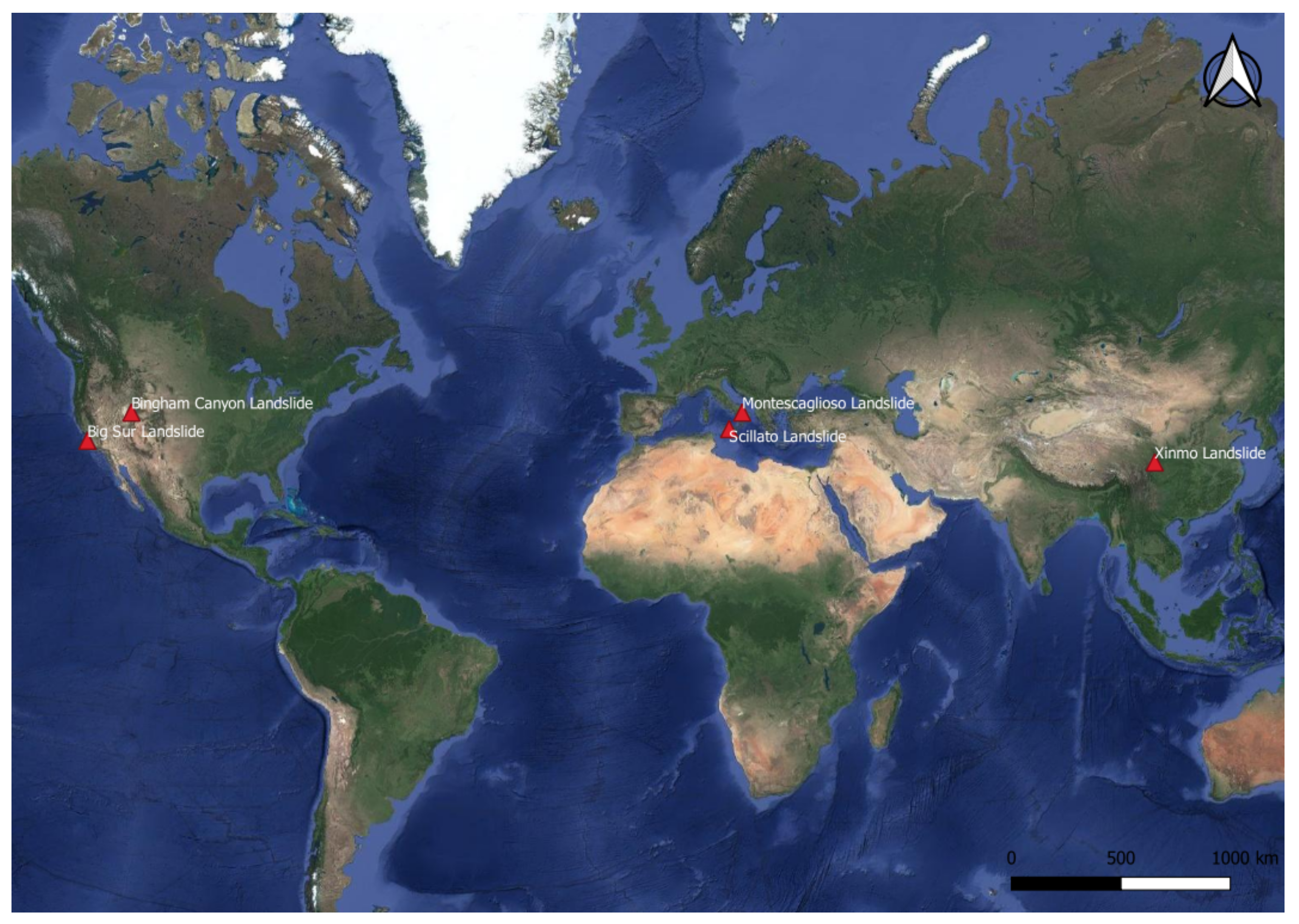
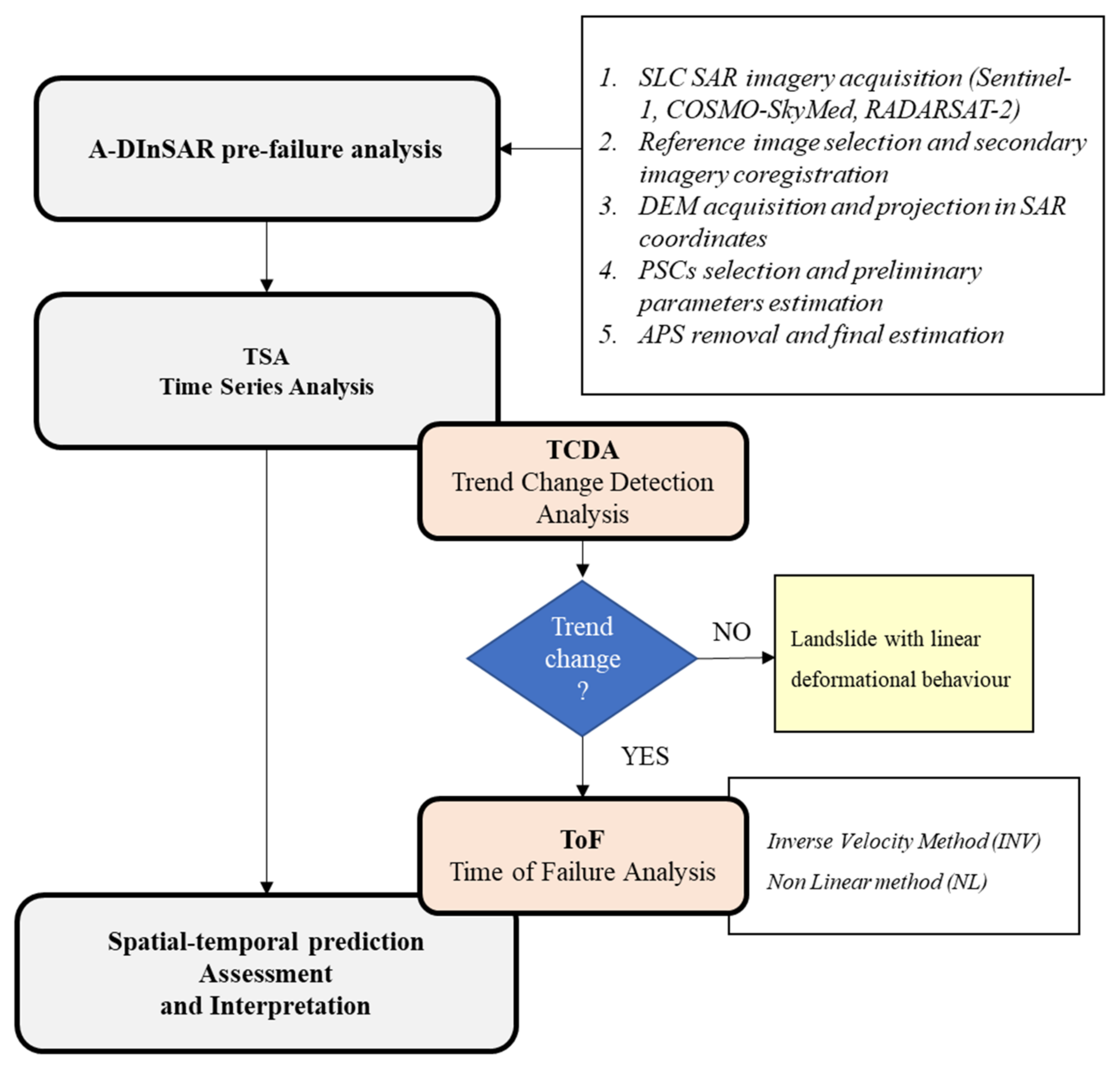
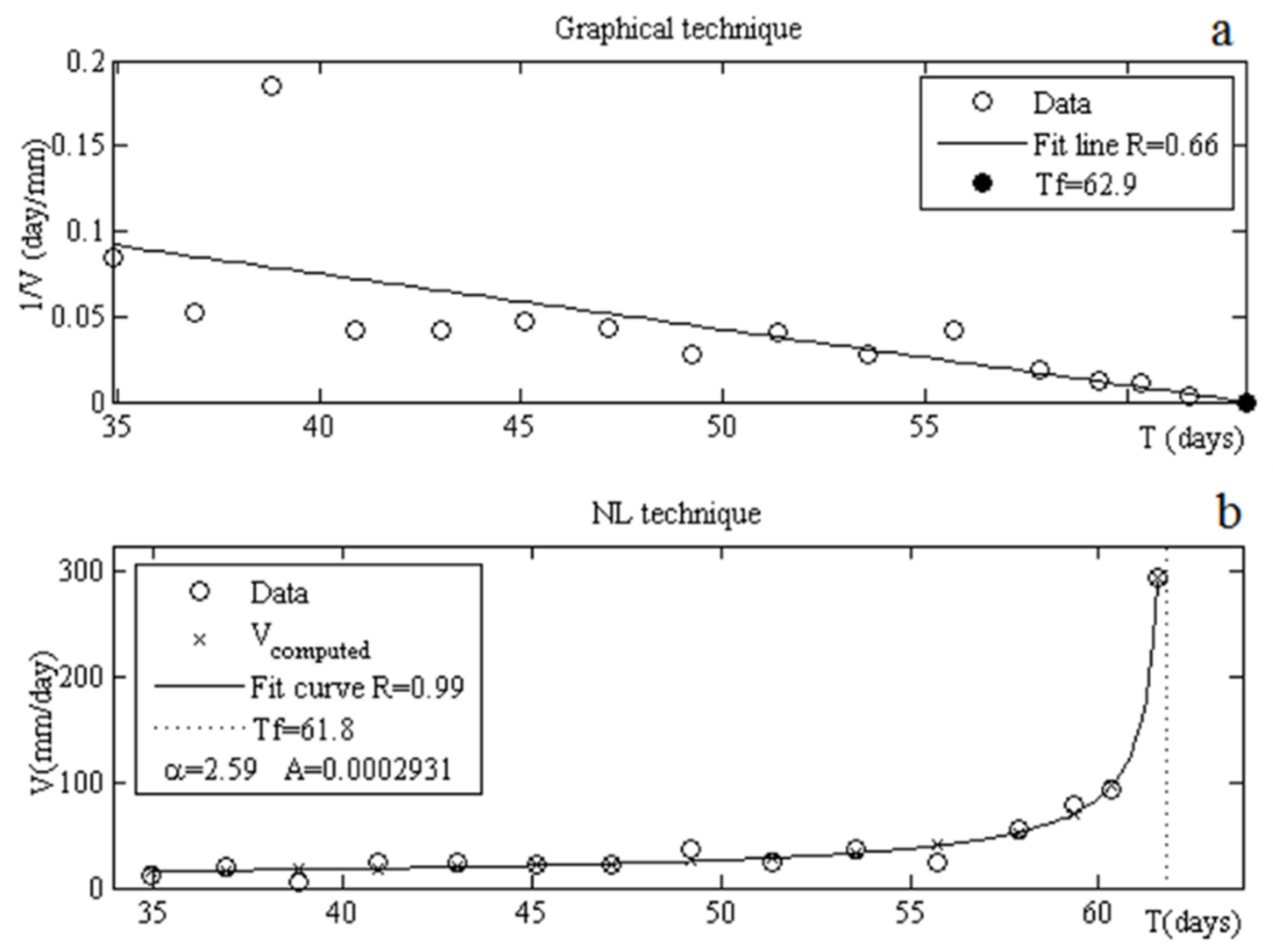
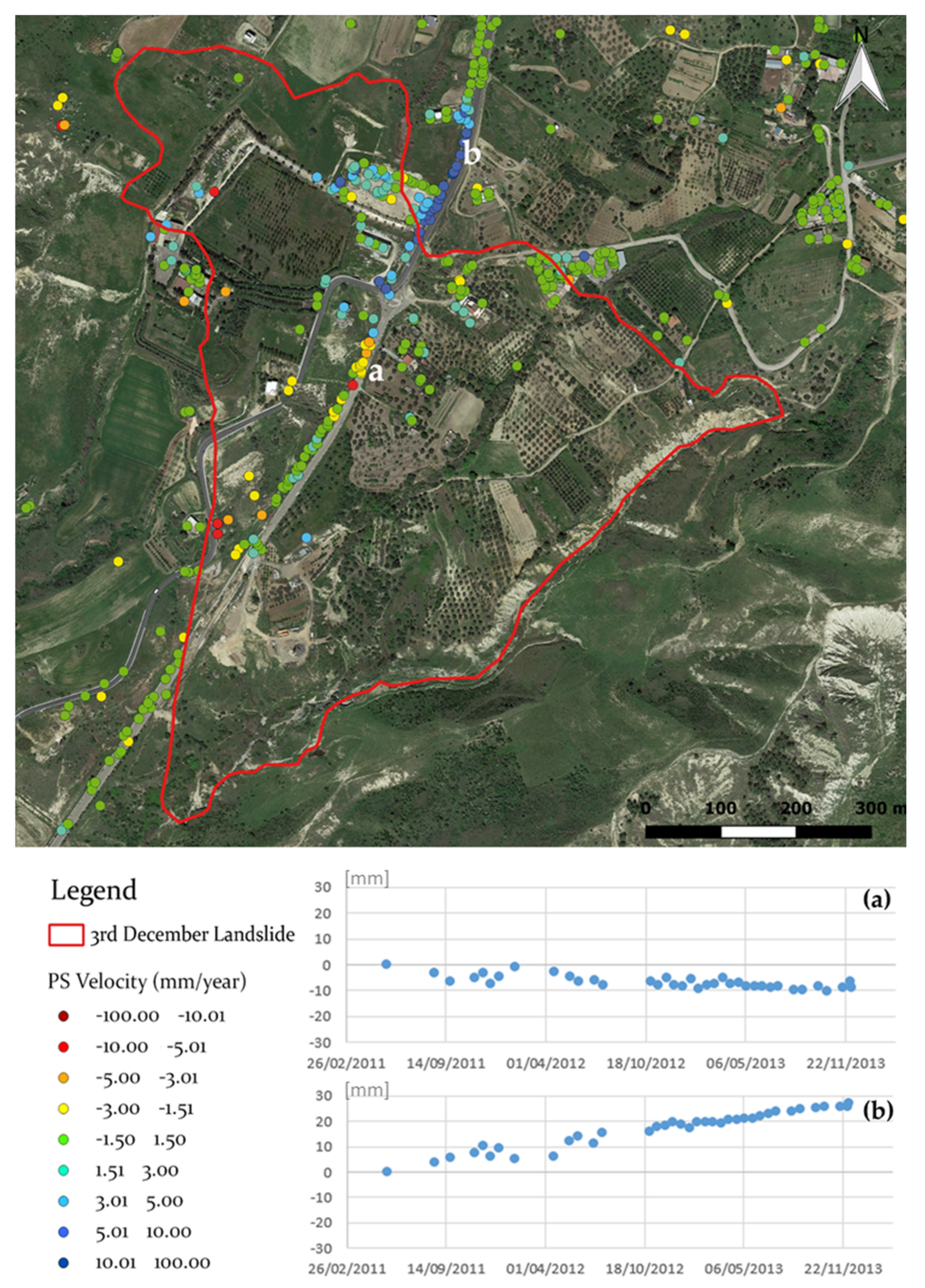
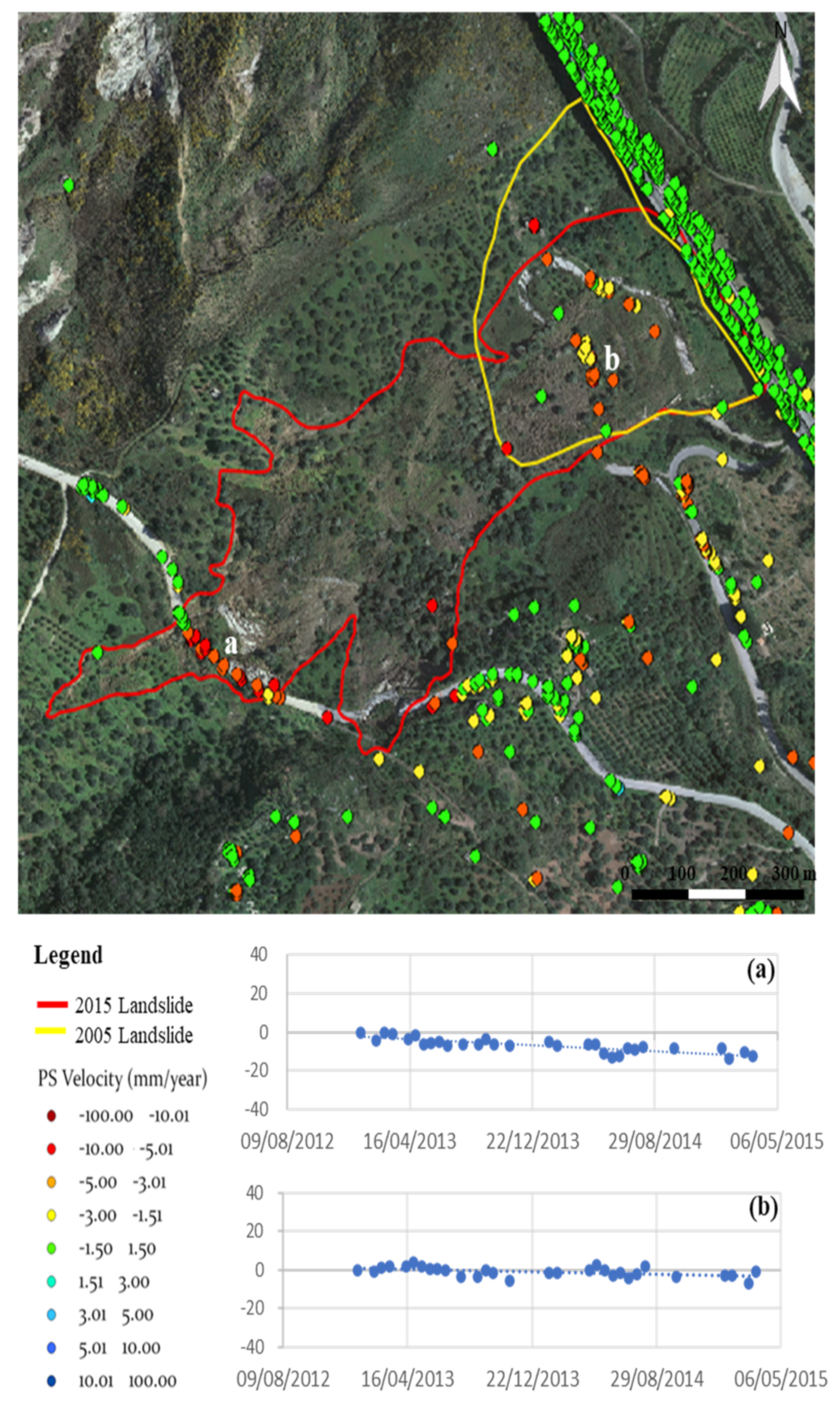
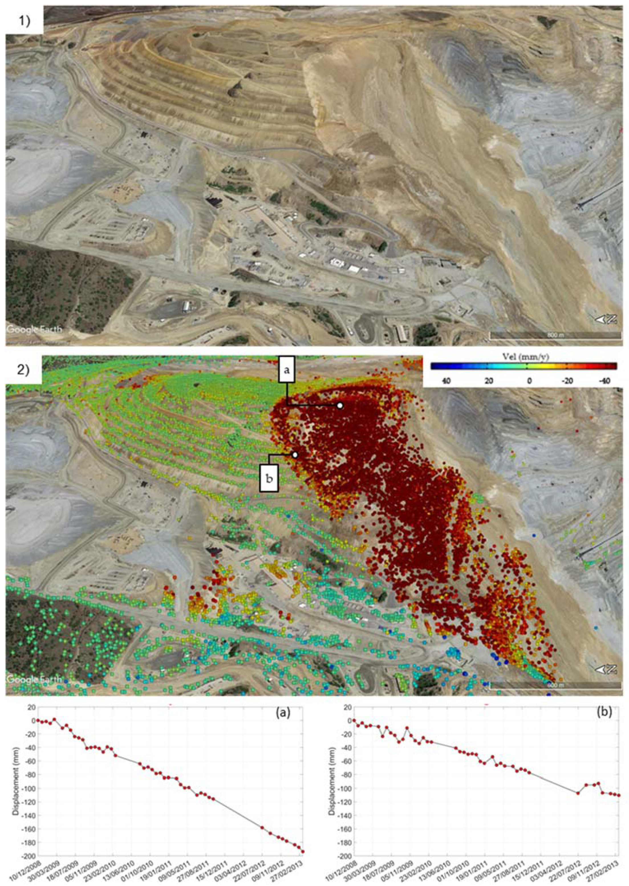
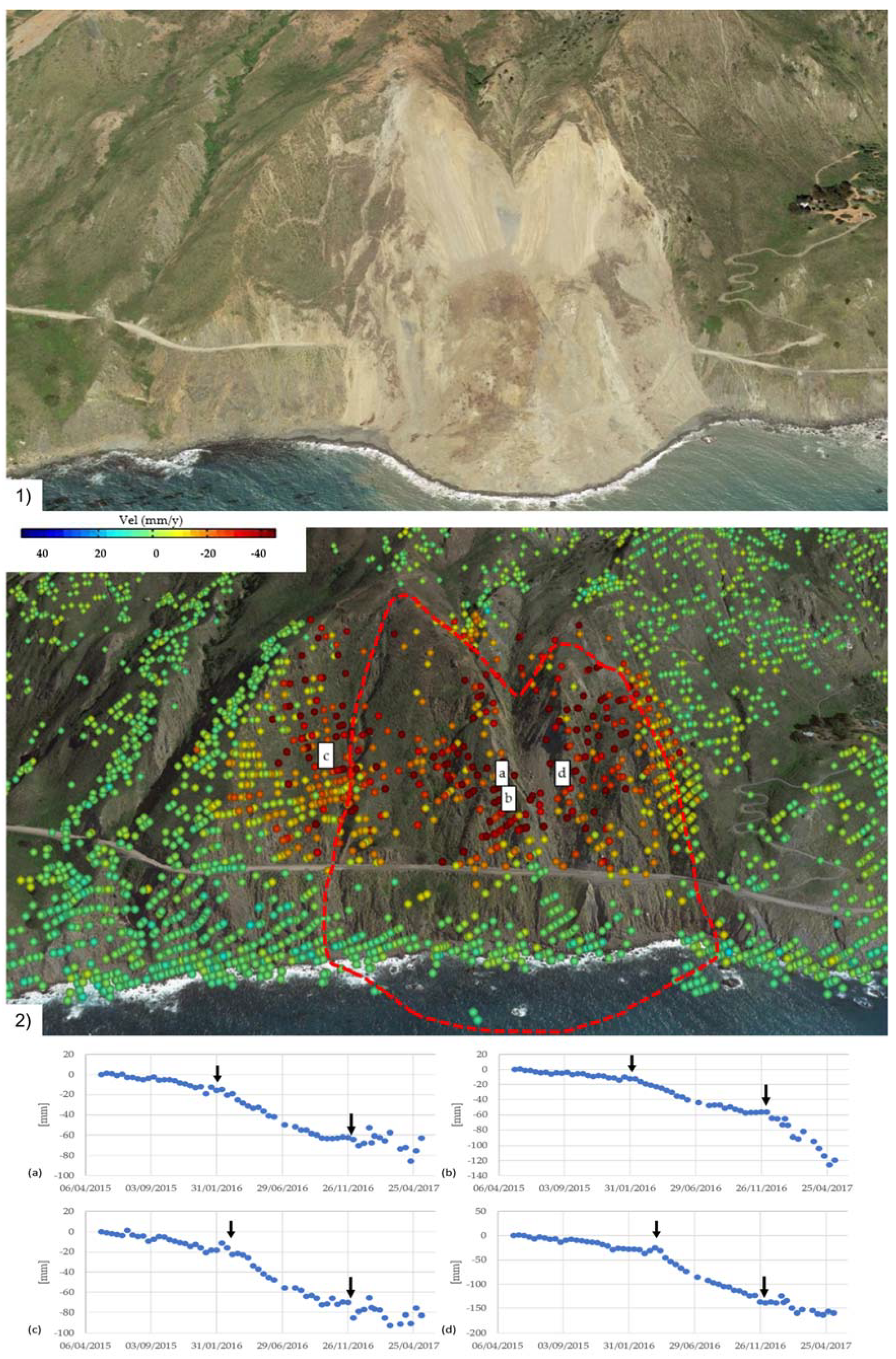
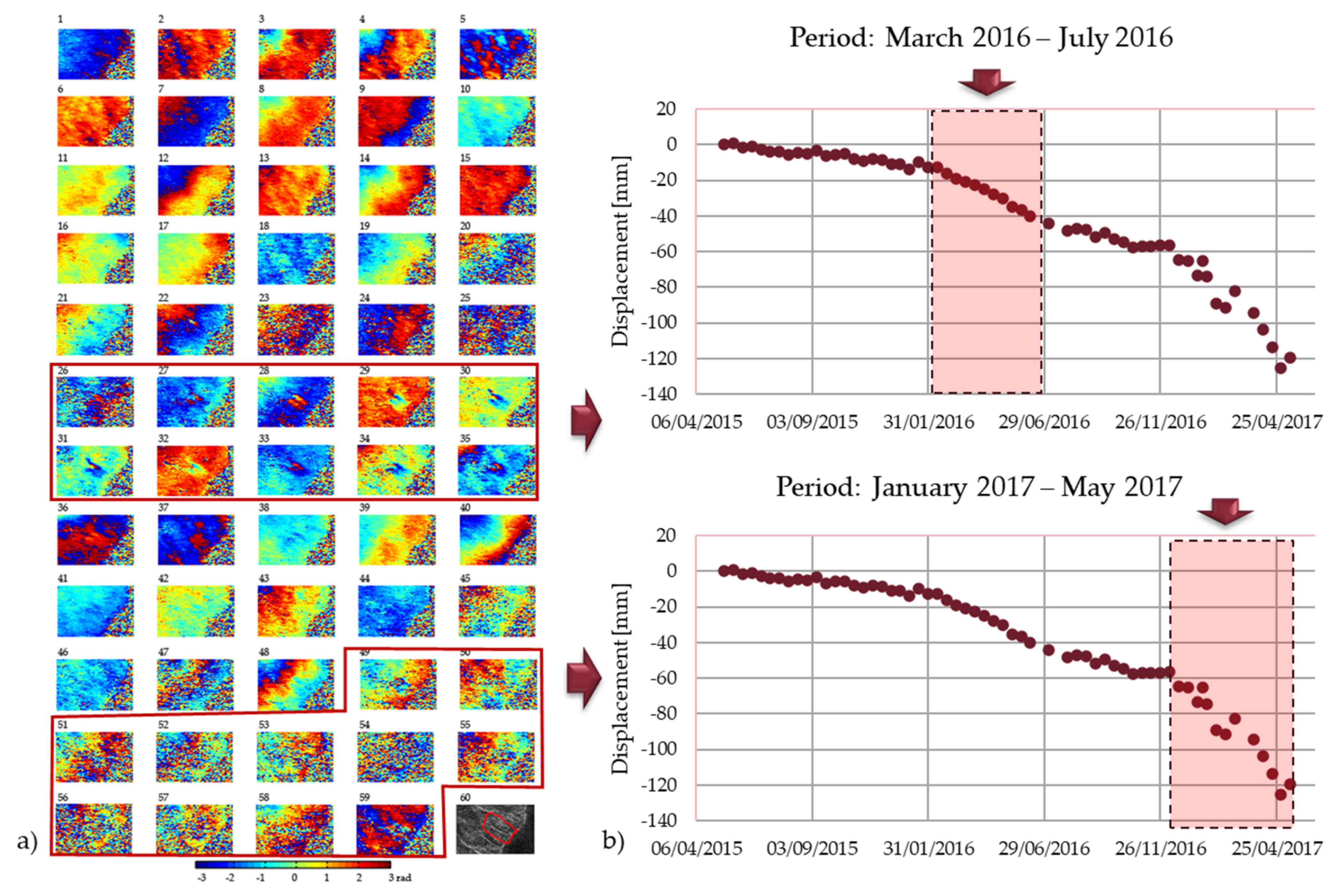
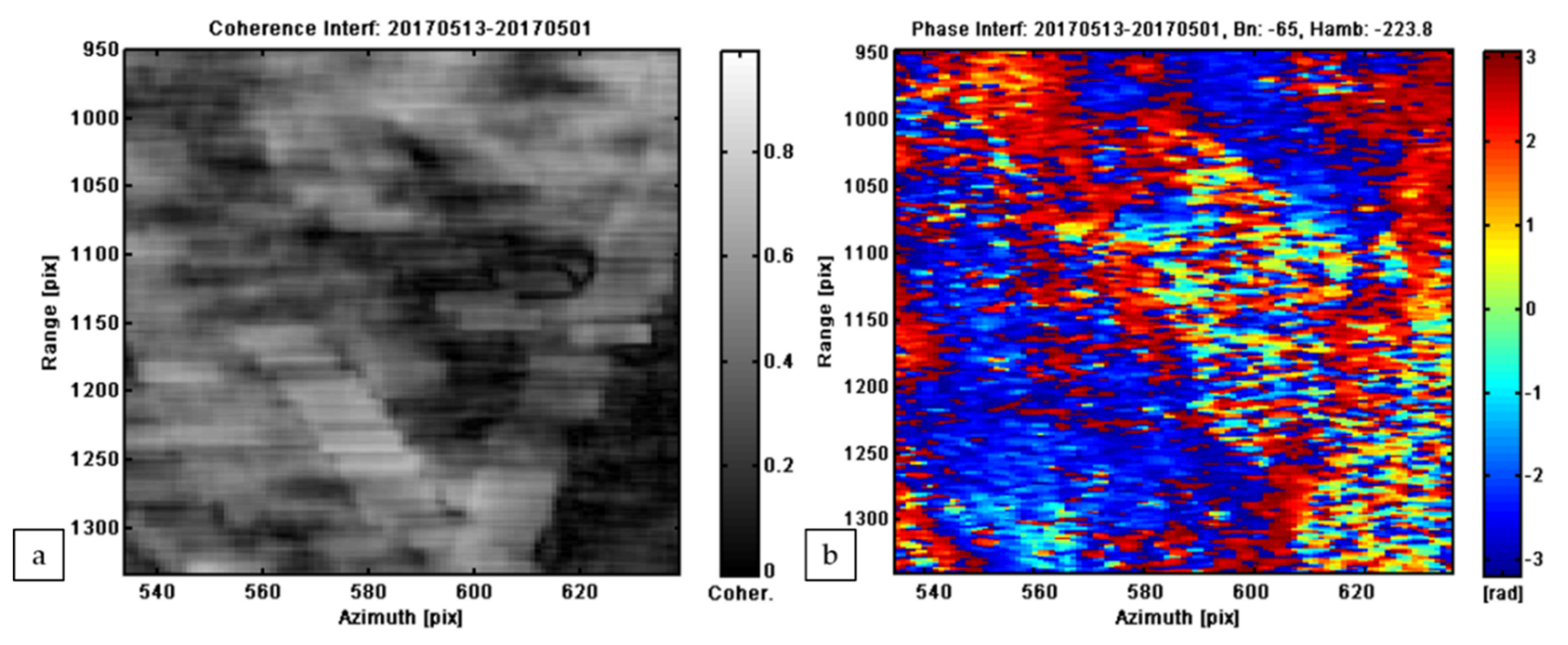
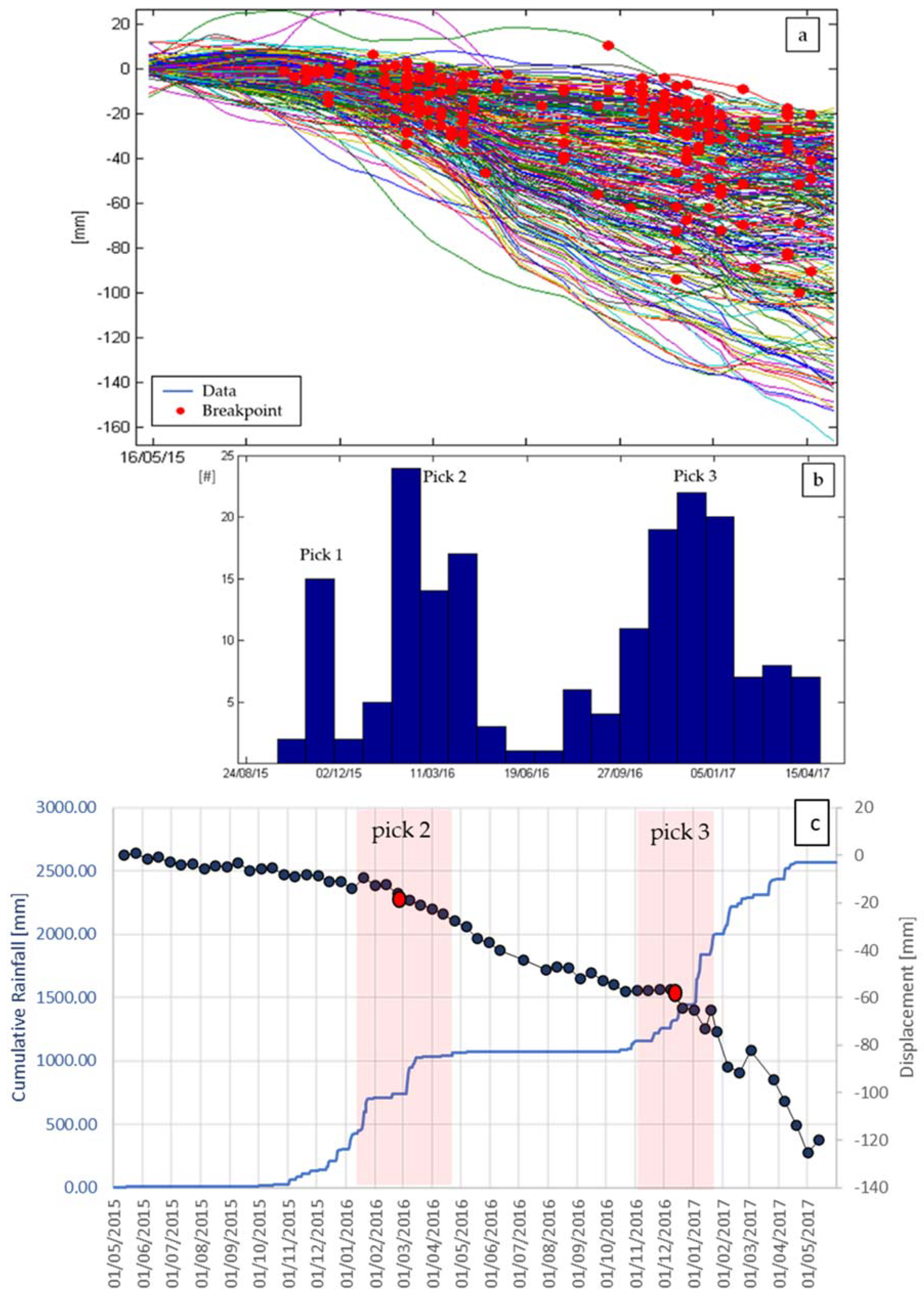
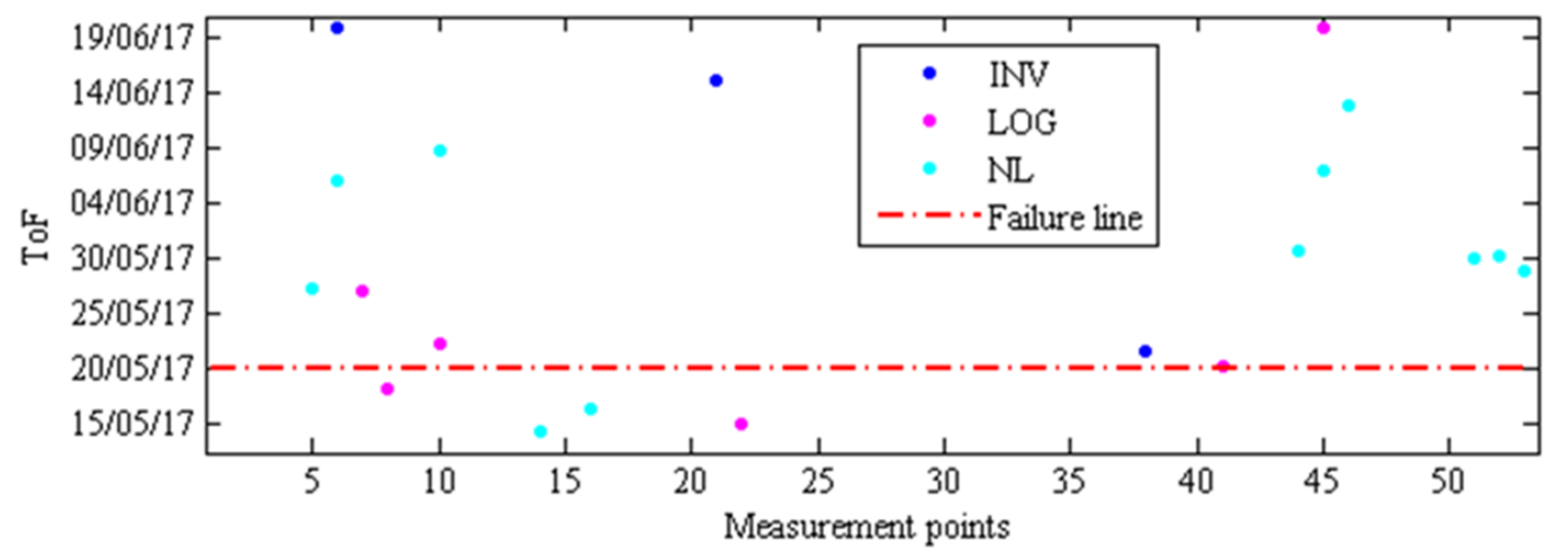
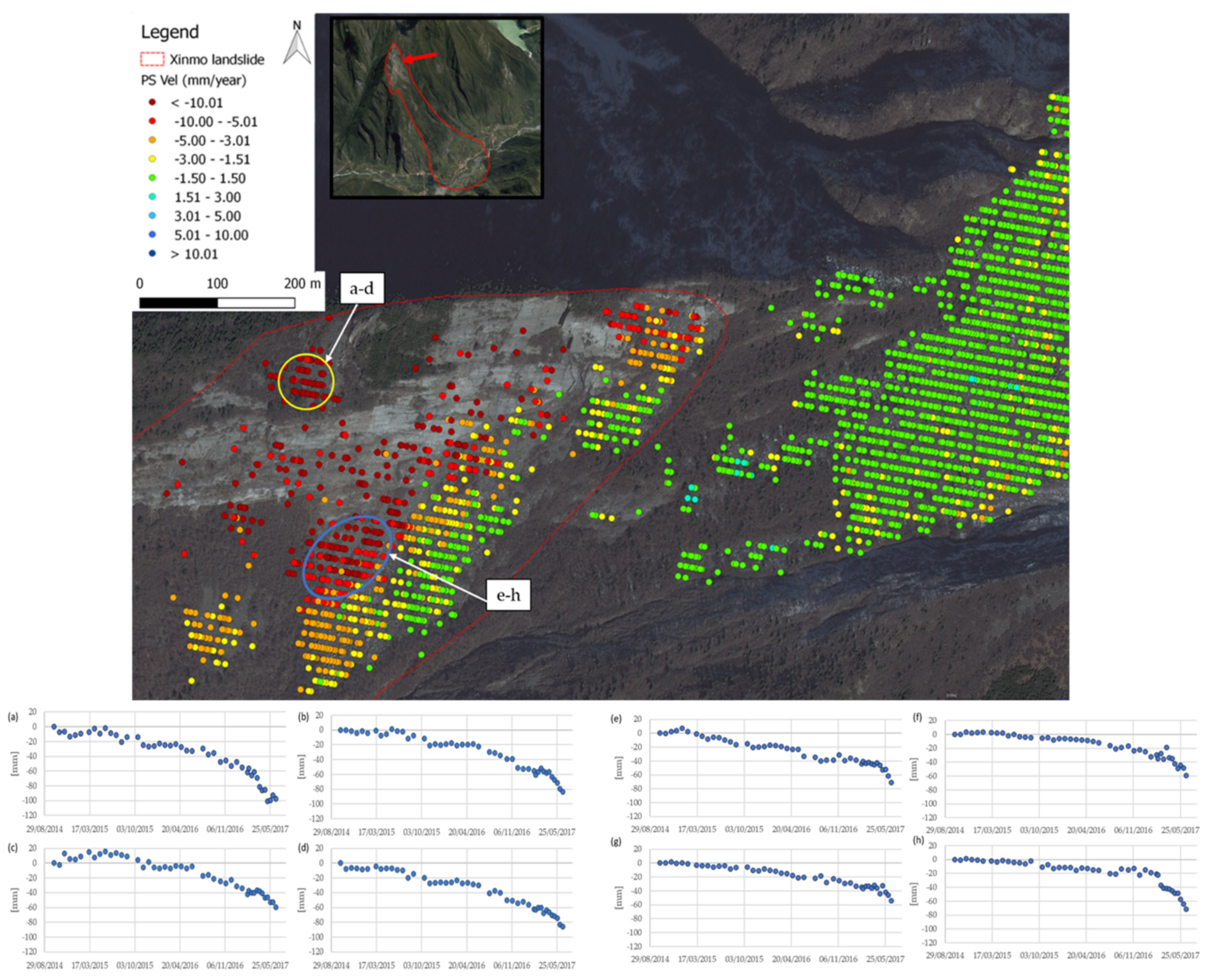
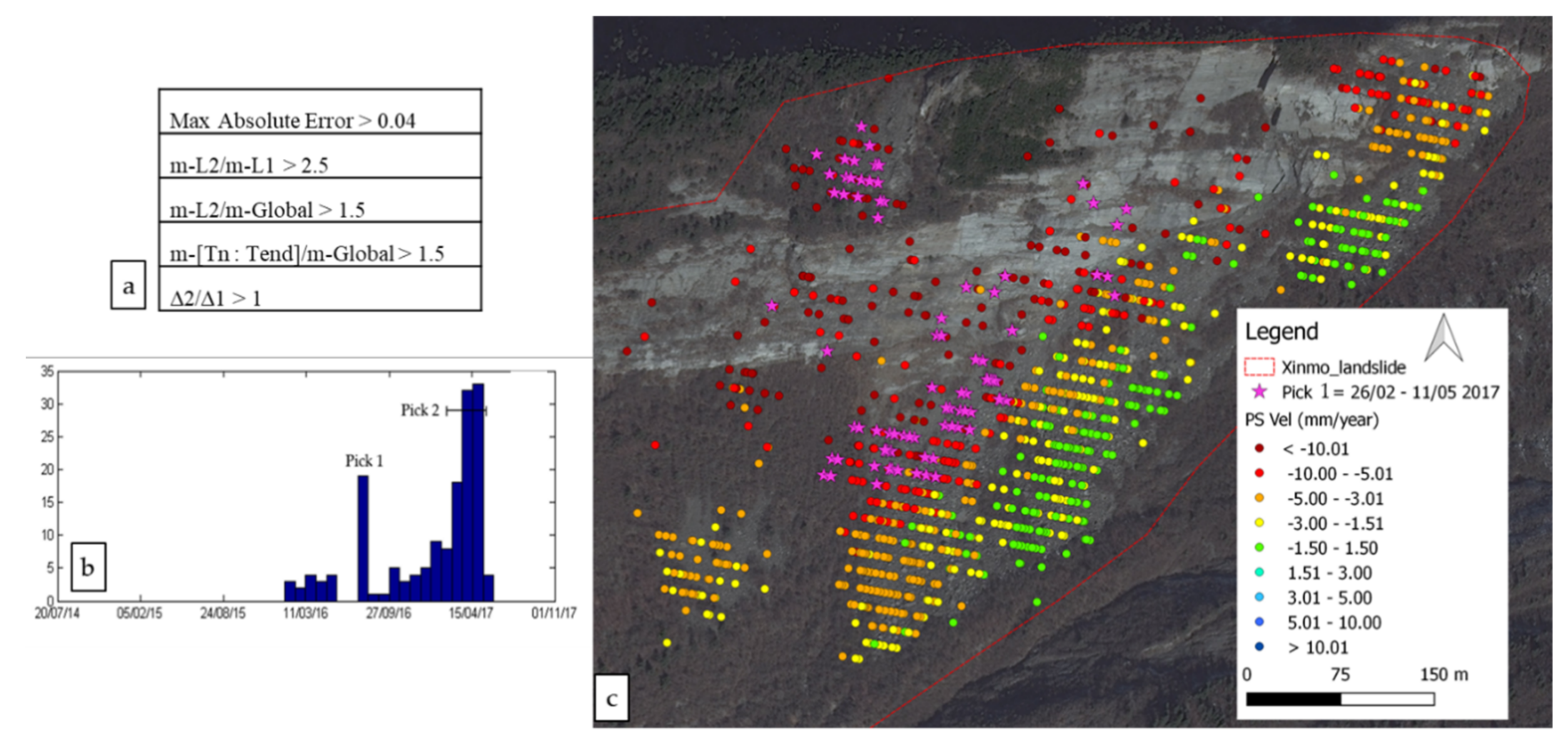
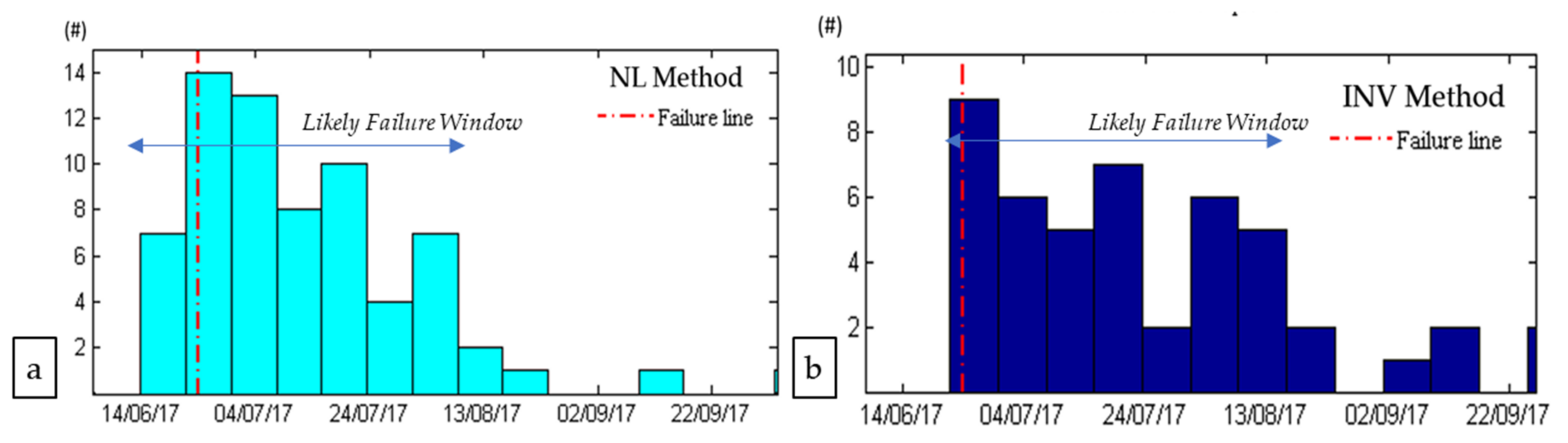
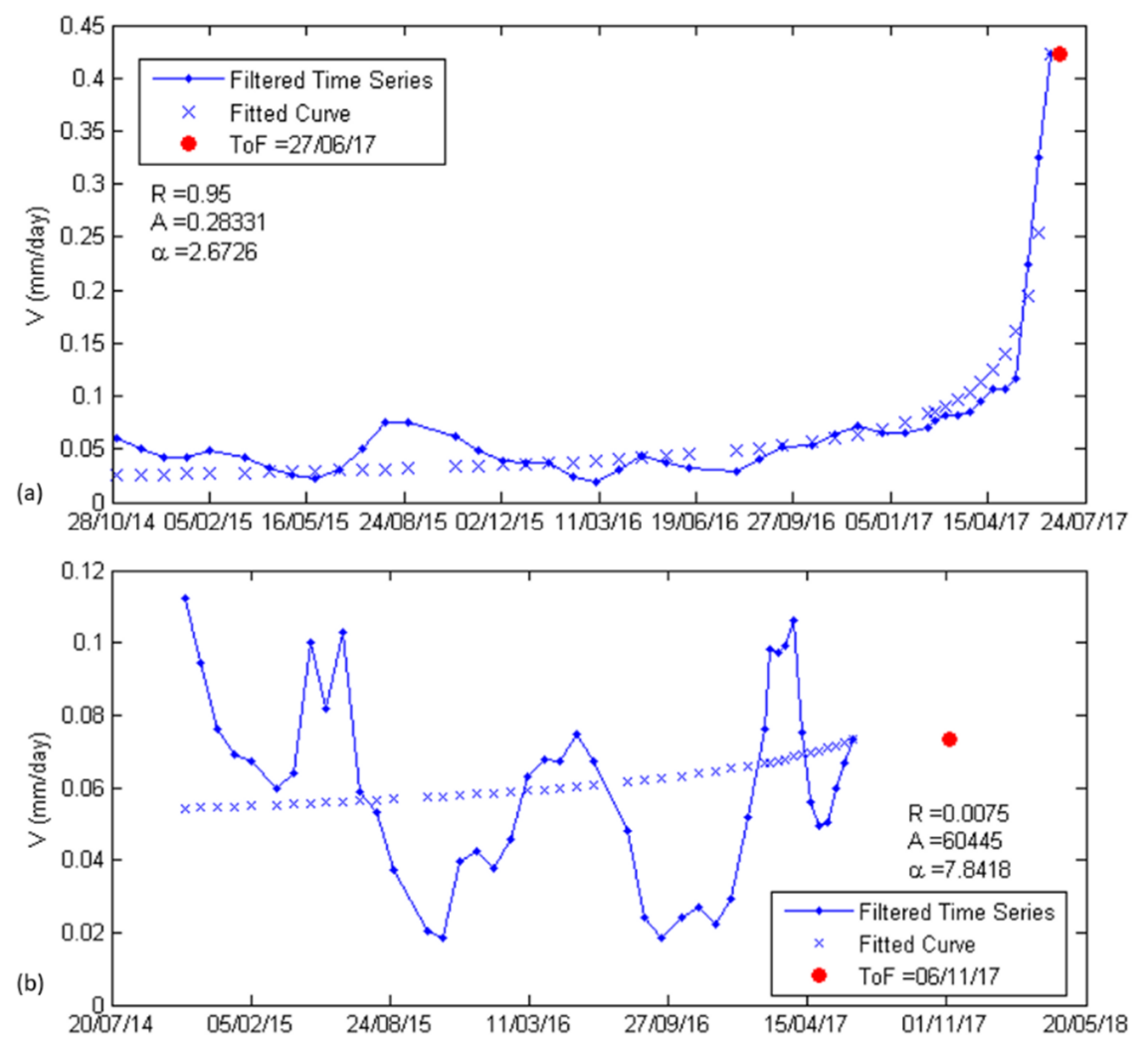
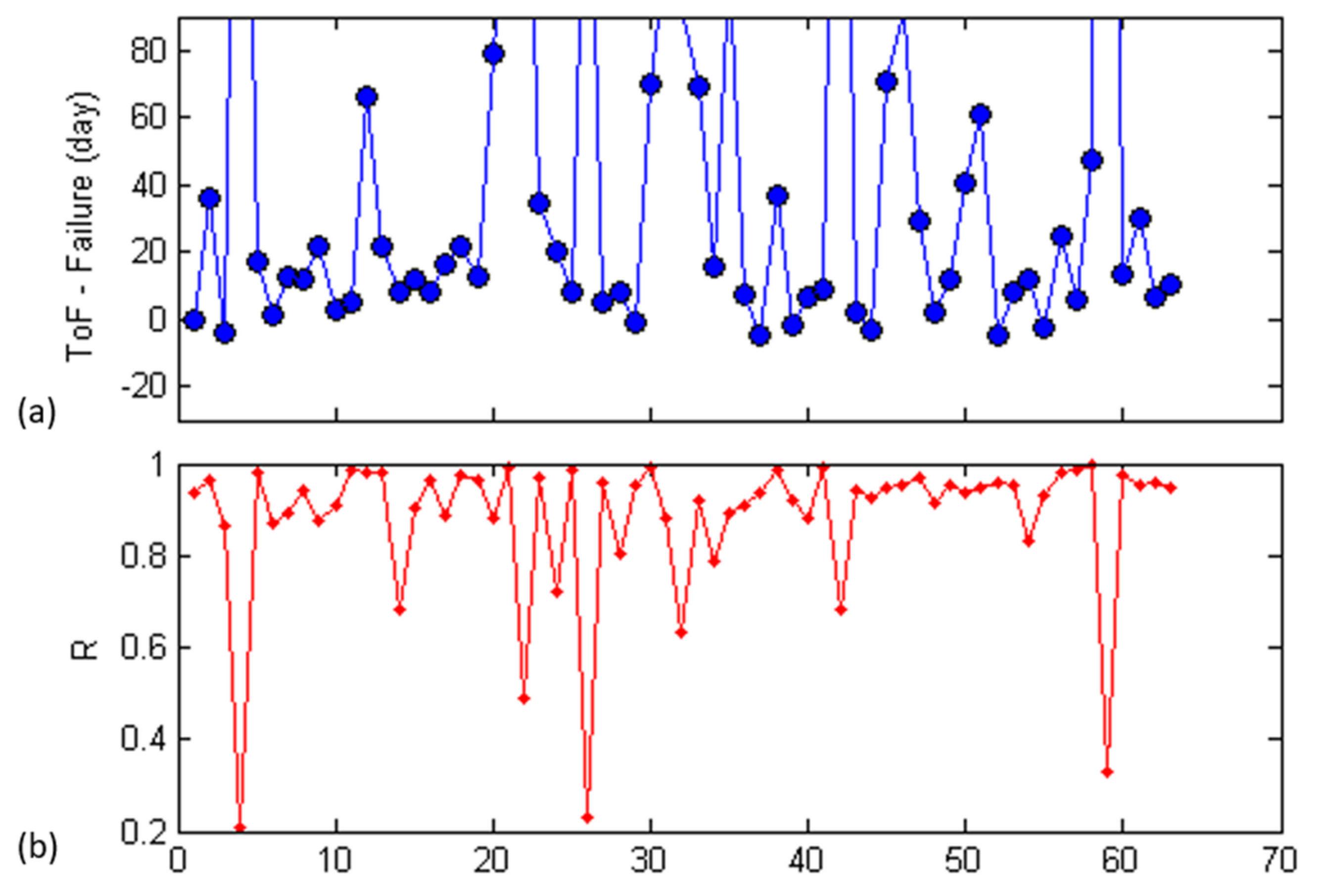
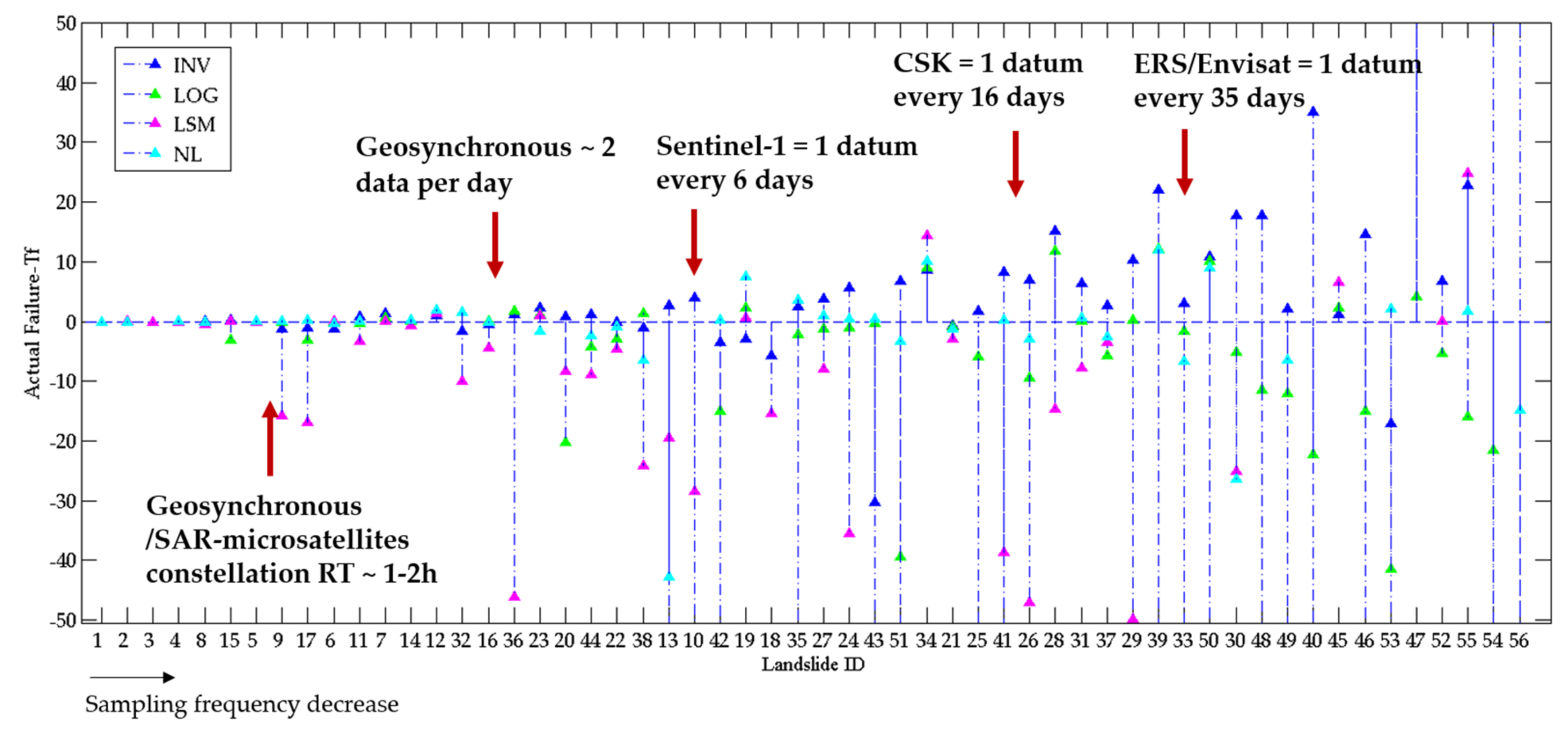
Table 1.
List of images used to generate the interferograms. The dates are presented in the following format: yyyymmdd. Bn is the normal baseline (in metres). TB is temporal baseline.
Table 1.
List of images used to generate the interferograms. The dates are presented in the following format: yyyymmdd. Bn is the normal baseline (in metres). TB is temporal baseline.
| Interferogram | Images | Bn | TB | Interferogram | Images | Bn | TB |
|---|---|---|---|---|---|---|---|
| 1 | 20150512–20150524 | 30.8812 | 12 | 31 | 20160506–20160518 | −67.3904 | 12 |
| 2 | 20150524–20150605 | 87.5209 | 12 | 32 | 20160518–20160530 | 18.2658 | 12 |
| 3 | 20150605–20150617 | −37.0054 | 12 | 33 | 20160530–20160611 | −17.3428 | 12 |
| 4 | 20150617–20150629 | 92.4879 | 12 | 34 | 20160611–20160705 | 94.8227 | 24 |
| 5 | 20150629–20150711 | −201.4874 | 12 | 35 | 20160705–20160729 | −103.4819 | 24 |
| 6 | 20150711–20150723 | 81.1978 | 12 | 36 | 20160729–20160810 | −46.1987 | 12 |
| 7 | 20150723–20150804 | 4.6342 | 12 | 37 | 20160810–20160822 | 94.9578 | 12 |
| 8 | 20150804–20150816 | −1.9977 | 12 | 38 | 20160822–20160903 | −36.6214 | 12 |
| 9 | 20150816–20150828 | 48.8288 | 12 | 39 | 20160903–20160915 | 28.5697 | 12 |
| 10 | 20150828–20150909 | −66.5864 | 12 | 40 | 20160915–20160927 | 49.1716 | 12 |
| 11 | 20150909–20150921 | −27.9898 | 12 | 41 | 20160927–20161009 | −34.5499 | 12 |
| 12 | 20150921–20151003 | 13.7339 | 12 | 42 | 20161009–20161021 | −47.3478 | 12 |
| 13 | 20151003–20151015 | 64.2993 | 12 | 43 | 20161021–20161102 | 85.6516 | 12 |
| 14 | 20151015–20151027 | −11.9484 | 12 | 44 | 20161102–20161114 | −4.1638 | 12 |
| 15 | 20151027–20151108 | −66.701 | 12 | 45 | 20161114–20161126 | −3.1614 | 12 |
| 16 | 20151108–20151120 | 25.107 | 12 | 46 | 20161126–20161208 | −49.8788 | 12 |
| 17 | 20151120–20151202 | 27.9885 | 12 | 47 | 20161208–20161220 | 19.321 | 12 |
| 18 | 20151202–20151214 | 69.8004 | 12 | 48 | 20161220–20170101 | 73.2145 | 12 |
| 19 | 20151214–20151226 | 17.9478 | 12 | 49 | 20170101–20170113 | −1.1805 | 12 |
| 20 | 20151226–20160107 | −73.5122 | 12 | 50 | 20170113–20170119 | −138.4077 | 6 |
| 21 | 20160107–20160119 | −38.7568 | 12 | 51 | 20170119–20170125 | 93.8401 | 6 |
| 22 | 20160119–20160131 | −18.7675 | 12 | 52 | 20170125–20170206 | −25.978 | 12 |
| 23 | 20160131–20160212 | 9.8419 | 12 | 53 | 20170206–20170218 | −69.1927 | 12 |
| 24 | 20160212–20160224 | 63.6508 | 12 | 54 | 20170218–20170302 | −27.3675 | 12 |
| 25 | 20160224–20160307 | 14.2739 | 12 | 55 | 20170302–20170326 | 117.0545 | 24 |
| 26 | 20160307–20160319 | −42.3275 | 12 | 56 | 20170326–20170407 | −35.8385 | 12 |
| 27 | 20160319–20160331 | −54.7575 | 12 | 57 | 20170407–20170419 | −28.6252 | 12 |
| 28 | 20160331–20160412 | −1.3179 | 12 | 58 | 20170419–20170501 | 14.1309 | 12 |
| 29 | 20160412–20160424 | 67.9668 | 12 | 59 | 20170501–20170513 | 64.8533 | 12 |
| 30 | 20160424–20160506 | 8.2471 | 12 |
Table 2.
Thresholds used as the stopping criteria where, for an anchor point located in i, m-L2 is the slope of the line that approximates the five data points after the anchor point; m-L1 is the slope of the line that fits the five points to the left of the anchor; m-Global is the angular coefficient of the regression line approximating the whole time series; m-[Ti : Tend] ism-L2 the slope of the regression line related to the data from T = i to the last T value; ∆2 is the gradient between the points i-1 and i; ∆1 is the gradient between the points i-2 and i-1. If all the constraints are met, a breakpoint is defined at the position i-1.
| Max Absolute Error > 0.04 |
| m-L2/m-L1 > 2.5 |
| m-L2/m-Global > 1.3 |
| m-[Tn : Tend]/m-Global > 1.1 |
| ∆2/∆1 > 1 |
Publisher’s Note: MDPI stays neutral with regard to jurisdictional claims in published maps and institutional affiliations. |
© 2021 by the authors. Licensee MDPI, Basel, Switzerland. This article is an open access article distributed under the terms and conditions of the Creative Commons Attribution (CC BY) license (https://creativecommons.org/licenses/by/4.0/).
Share and Cite
MDPI and ACS Style
Moretto, S.; Bozzano, F.; Mazzanti, P. The Role of Satellite InSAR for Landslide Forecasting: Limitations and Openings. Remote Sens. 2021, 13, 3735. https://0-doi-org.brum.beds.ac.uk/10.3390/rs13183735
AMA Style
Moretto S, Bozzano F, Mazzanti P. The Role of Satellite InSAR for Landslide Forecasting: Limitations and Openings. Remote Sensing. 2021; 13(18):3735. https://0-doi-org.brum.beds.ac.uk/10.3390/rs13183735
Chicago/Turabian StyleMoretto, Serena, Francesca Bozzano, and Paolo Mazzanti. 2021. "The Role of Satellite InSAR for Landslide Forecasting: Limitations and Openings" Remote Sensing 13, no. 18: 3735. https://0-doi-org.brum.beds.ac.uk/10.3390/rs13183735
Note that from the first issue of 2016, this journal uses article numbers instead of page numbers. See further details here.