
An Application of Sea Ice Tracking Algorithm for Fast Ice and Stamukhas Detection in the Arctic


1
N. N. Zubov State Oceanographic Institute, Roshydromet, Kropotkinskij per. 6, 119034 Moscow, Russia
2
Nansen Environmental and Remote Sensing Centre, Thormøhlens Gate 47, 5006 Bergen, Norway
3
Arctic and Antarctic Research Institute, ul. Beringa 38, 199397 St. Petersburg, Russia
4
Nansen International Environmental and Remote Sensing Center, 199034 St. Petersburg, Russia
*
Author to whom correspondence should be addressed.
†
These authors contributed equally to this work.
Remote Sens. 2021, 13(18), 3783; https://0-doi-org.brum.beds.ac.uk/10.3390/rs13183783
Submission received: 21 July 2021
/
Revised: 15 September 2021
/
Accepted: 16 September 2021
/
Published: 21 September 2021
(This article belongs to the Section Remote Sensing Communications)
Abstract
:For regional environmental studies it is important to know the location of the fast ice edge which affects the coastal processes in the Arctic. The aim of this study is to develop a new automated method for fast ice delineation from SAR imagery. The method is based on a fine resolution hybrid sea ice tracking algorithm utilizing advantages of feature tracking and cross-correlation approaches. The developed method consists of three main steps: drift field retrieval at sub-kilometer scale, selection of motionless features and edge delineation. The method was tested on a time series of C-band co-polarized (HH) ENVISAT ASAR and Sentinel-1 imagery in the Laptev and East Siberian Seas. The comparison of the retrieved edges with the operational ice charts produced by the Arctic and Antarctic Research Institute (Russia) showed a good agreement between the data sets with a mean distance between the edges of <15 km. Thanks to the high density of the ice drift product, the method allows for detailed fast ice edge delineation. In addition, large stamukhas with horizontal size of tens of kilometers can be detected. The proposed method can be applied for regional fast ice mapping and large stamukhas detection to aid coastal research. Additionally, the method can serve as a tool for operational sea ice mapping.

1. Introduction
Fast ice is sea ice adjacent to the coast which lacks motion for a certain period [1]. Fast ice is an important component of the Arctic coastal environment. Fast ice forms seasonally in the majority of the Arctic marginal seas. Multiyear fast ice is an exceptional phenomenon in the Arctic. Its occurrence is limited to the Canadian Archipelago [2], parts of the Taymyr Peninsula [3] and Greenland [4]. In [5], Zubov describes fast ice development as a process of dynamic attachments of ice flows to the land or seaward fast ice edge: The onshore winds push ice towards the fast ice edge where it undergoes hummocking and freezes to fast ice. During its formation under the pressure of drifting ice, fast ice often breaks, forming a series of hummocks and stamukhas (grounded ridged ice features). By April–May, fast ice usually reaches its maximal winter extent. It varies strongly on a regional scale from tens of kilometers wide along Alaska’s coast to hundreds of kilometers in the Laptev and East Siberian Seas. The fast ice plays an important role in the interaction of ice cover with the coastal zone and the adjacent land. The formation of stamukhas, which ground at the bottom, in turn, plays an important role in the stability of the fast ice. Due to climate change, fast ice begins to form later and breaks up earlier [6]. As a result, the duration of the fast ice season becomes shorter [6,7,8]. In addition, the frequency of fast ice mid-winter breakout events increases [9,10]. Due to the shortening of the fast ice season, wave action and wind at the shoreline increase, which in turn leads to a higher rate of coastal erosion and accelerated coastal retreat [11,12]. Grounded sea ice ridges and stamukhas also play an important role in the Arctic coastal dynamic [13,14]. Leaving gouges at the bottom, the grounded sea ice features threaten damage to the offshore infrastructure [15]. Furthermore, monitoring of sea ice in the coastal areas is a crucial task for modeling and prediction of sea ice conditions.
For operational purposes and climatology observations, fast ice is mapped by sea ice experts manually from a time series of available satellite data. The Arctic-wide sea ice maps are issued on a weekly or bi-weekly basis, e.g., sea ice charts produced by the Arctic and Antarctic Research Institute (Russia) and the U.S. National Ice Center. There are also a variety of techniques to map fast ice (semi-)automatically. Most of the existing methods define fast ice as sea ice cover experiencing no changes in its surface characteristic [1,16,17,18,19,20,21,22]. Unlike optical data used in [16,20], Synthetic Aperture Radar (SAR) data can be used independently from weather and solar insulation conditions. Reasonable spatiotemporal coverage along with high spatial resolution make SAR an important tool for sea ice condition mapping in the Arctic. Fast ice extent and stability are mapped by means of L- and C-band SAR interferometry (InSAR) [17,19] with high accuracy and robustness. However, long temporal separation between the repeated image pairs does not allow using the method for operational purposes. Karvonen [18] developed and tested a fast ice detection method for the Kara Sea region using correlation analysis on successive Sentinel-1 C-band images for operational purposes. The method allows mapping fast ice in the region every 15 days. The authors of [23] mapped Antarctic fast ice using a cross-correlation technique to search for near-zero displacement with C-band RADARSAT-1 imagery. With this paper, we exploit the idea to use the near zero-displacement criterion for fast ice mapping in the Arctic. In this study we aim to increase the resolution of the detected fast ice edge by using a fine-resolution sea ice drift product.
To follow and develop the idea of using SAR-derived ice drift products for fully automated and accurate fast ice zone mapping, we suggest an improved sea ice drift retrieval approach. The core idea is to combine the advantages of state-of-the-art sea ice drift algorithms to derive dense and robust ice displacement vectors that can be then used as input for fast ice delineation and stamukhas detection. Compared to similar methods presented in [17,18,20], we attempt to take a step forward in automated fast ice mapping by usage of a combination of feature-tracking and cross-correlation techniques to increase the robustness and spatial resolution of the final product. It should be noted that in some cases the ice drift algorithms could produce some amount of erroneous ice displacement vectors that significantly decrease the robustness and quality of the derived products [24], therefore, special attention should be paid to erroneous vectors filtering.
In this study we introduce automatic edge extraction in order to minimize manual editing and reduce subjectivity in the detection of fast ice zones and stamukhas by using an improved sea ice drift retrieval approach. Robustness and accuracy evaluation of the proposed approach is performed in two test sites in the Laptev and East Siberian Seas which are characterized by variable fast ice regime. The applicability of the method is tested on co-polarised (HH) SAR images acquired from ENVISAT ASAR and Sentinel-1 C-band SAR space-born sensors.
2. Materials and Methods
2.1. SAR Image Pairs
SAR data are very useful for regional sea ice monitoring. Two of the main advantages of active microwave remote sensing are the high spatial resolution achievable (1–100 m) and the ability to image the Earth’s surface at both day and night in almost all weather conditions. In our study we used a time series of consecutive C-band SAR images acquired in wide-swath mode at HH polarization by ENVISAT and Sentinel-1 satellites. The uncalibrated and ungeocoded images were selected and downloaded from the Alaska Satellite Facility (ASF) web-server. The raw image intensity values were calibrated and converted to dB, and then projected onto the Universal Polar Stereographic (UPS) grid with a pixel size of 150 and 40 ground meters for ENVISAT and Sentinel-1, correspondingly. Overall, we processed 6 pairs with time gaps from 1 to 3 days of ENVISAT images taken between 13 and 25 December 2007 in the Laptev Sea region and 4 pairs of Sentinel-1 images taken between 19 January and 22 February 2016 in the East Siberian Sea. The selected time intervals cover periods with variable configurations of the fast ice edge.
2.2. Operational Sea Ice Charts
For the cross-comparison we used sea ice charts produced by the Arctic and Antarctic Research Institute (AARI). The weekly charts were used. The fast ice is mapped manually by sea ice experts based on the mutual analysis of the available satellite and in-situ data. A chart represents mean sea ice conditions of the period of 2–5 days before the issue.
2.3. Fast Ice Edge Delineation
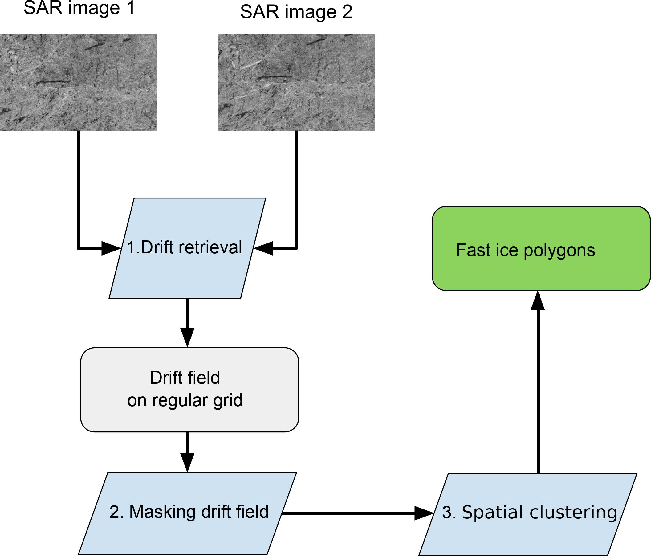
To detect fast ice we proposed the following algorithm, which comprises: 1—sea ice drift retrieval, 2—masking of the resultant drift field, and 3—spatial clustering (Figure 1). Each step is described below.
- 1.
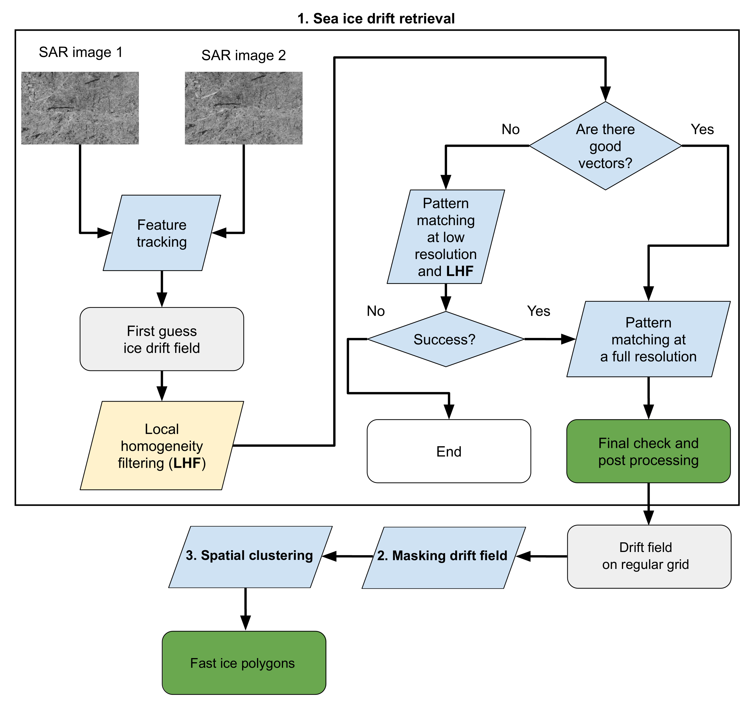
- Sea ice drift retrieval.We designed and implemented an advanced hybrid ice drift algorithm for robust sea ice drift retrieval using a sequence of SAR images at near sub-kilometer scale. The core part of our method is the SAR sea ice tracking approach proposed in [25] aiming to track distinguishable sea ice features throughout a sequence of images with sub-pixel accuracy. However, when the SAR sea ice signal is homogeneous, the features become indistinct, thus, the feature-based algorithms such as [25] could fail. Another limitation of the algorithms is sparse output data. In these cases, the area-based methods operating with the intensity values of image patches are preferable [26]. To combine the benefits of both types of retrieval approaches we developed a hybrid ice drift framework based on the feature tracking algorithm [25] and the normalized cross-correlation technique [27]. Here, and throughout the text, we refer to the area-based normalized cross-correlation technique as to the pattern matching. A full algorithm workflow is shown in Figure 1. In the initial attempt, we estimate the ice displacement by the feature tracking algorithm with default parameters described in [25]. Then we apply the local homogeneity criteria [25] for the obtained ice drift field to determine whether ’good’ ice drift vectors are present. A sea ice displacement vector is considered as a true vector if the following criteria are satisfied:
- a vector has at least 7 neighbors in a radius of 300 pixels;
- a vector has at least 5 neighbors with similar directions that deviate from the considered within 5;
- a vector has at least 5 neighbors with the length varying within 3 pixels from the concerned.
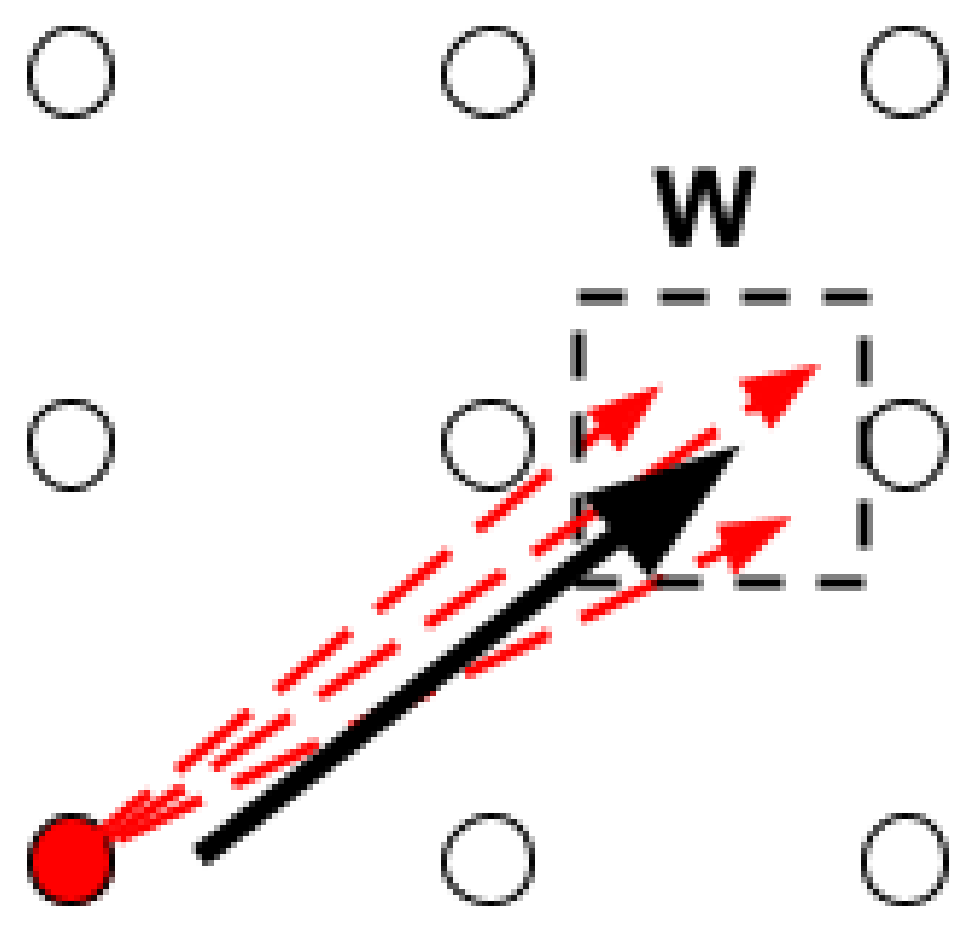
The criteria thresholds were defined empirically and based on the assumption that several vectors should ’belong’ to a certain ice floe that survived a period between acquisitions of SAR images, and thus both their length and direction must be homogeneous. These simple and consistent criteria allow to keep only feasible ice drift vectors, including those determined in the zones with large ice speed gradients, such as near the borders between drifting and fast ice. The obtained ice drift vectors are sparsely distributed and, as mentioned above, it might not be possible to derive them at all in some cases. To overcome these obstacles, the area-based algorithm is used. If there are a number of the ’good’ ice displacement vectors produced by the feature tracking algorithm, they become the guide vectors for the pattern matching algorithm, which greatly reduces the computational efforts by decreasing the search area (see Figure 2).A pair selection for ice drift determination depends on SAR data availability. The time gap between the nearest SAR image acquisitions covering the same area of Arctic typically varies from 1 to 3 days for both Sentinel-1 and ENVISAT. To optimize the computational efficiency for pattern matching, we performed ice drift calculation on a coarse resolution first, and then on full-resolution grids. The derived ice drift vectors at coarse spatial resolution (the grid step size of 100 pixels) as the first guess allows to check if the true ice displacement vectors can be obtained. In case of successfully retrieved ice drift vectors, a computation is performed on a full resolution grid with a step size of 30 pixels that corresponds to 4.5 km and 1.2 km for ENVISAT and Sentinel-1 wide-swath data, respectively. An image patch size is set to 32 × 32 pixels and a default searching area size is of 500 × 500 pixels around a grid point. Therefore, the proposed ice drift retrieval approach that is a combination of the feature tracking and pattern matching utilizing the benefits of both allows us to obtain a robust ice drift product on a regular grid. At the final stage of the ice drift retrieval, the resultant ice displacement vectors are checked for the local homogeneity, and then used for further processing. Figure 2 shows an example of the resultant sea ice drift field obtained using the described approach. - 2.
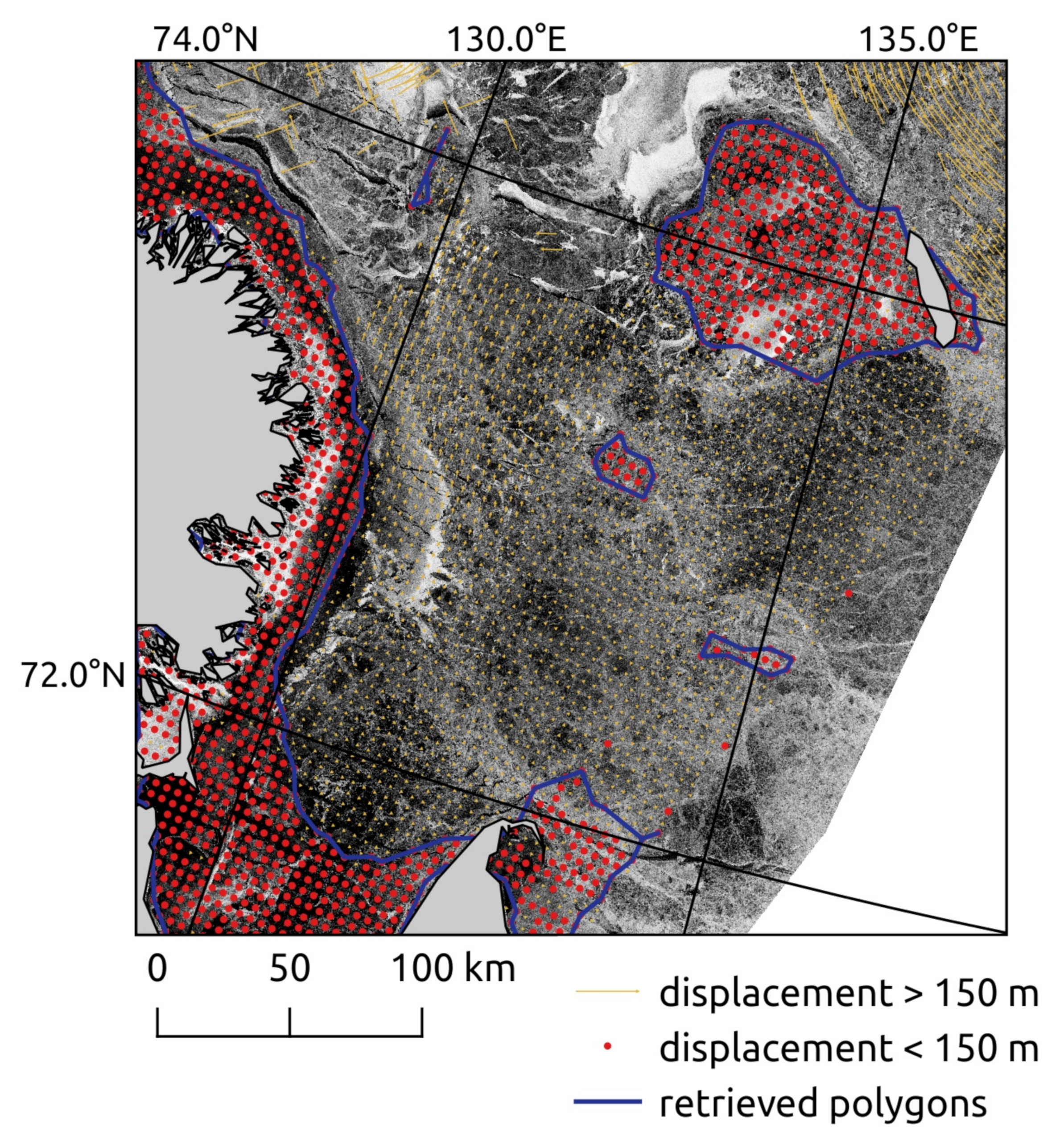
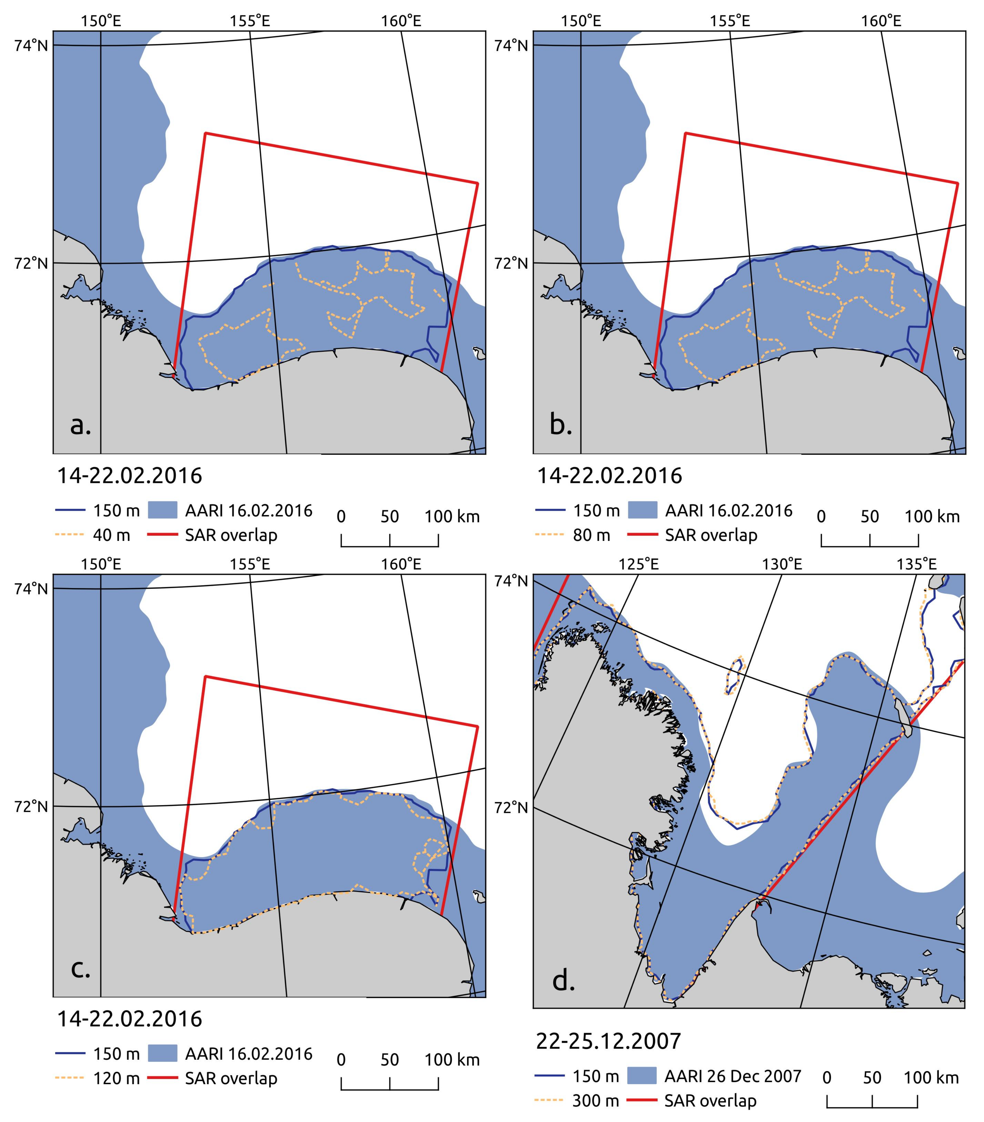
- Masking of the resultant drift fields.The sea ice drift field was masked by displacement so that only the point with displacement of less that 150 m remained (Figure 3). The displacement threshold was selected empirically. The algorithm was tested with 1-, 2- and 3-pixel displacement thresholds (40, 80 and 120 m correspondingly) for Sentinel-1 data (Figure A1a–c) and 1- and 2-pixel displacement threshold (150 and 300 m) for ENVISAT data (Figure A1d). For Sentinel-1 data, the best performance was obtained with a 3-pixel (120 m) threshold, while for the ENVISAT data both 1- and 2-pixel (150 and 300 m) thresholds showed almost identical results. For consistency, the displacement threshold was set to 150 m for both Sentinel-1 and ENVISAT data. Additionally, the land features are masked at this step using a GSHHG landmask L1 (https://www.soest.hawaii.edu/pwessel/gshhg/ (accessed on 27 April 2021)). Therefore, the resultant group of points correspond to motionless fast ice or stamukhas.
- 3.
- Spatial clustering.To draw the contours of the field with no displacement we used the alpha-shape method of computational geometry applied in [28]. The method creates the space generated by point pairs that can be touched by an empty disc of radius alpha. The alpha parameter controls the level of details of the obtained contour.
The output of the proposed algorithm is a set of lines delineating polygons of motionless sea ice cover, i.e., fast ice, stamukhas surrounded by fast ice and large stamukhas. The accuracy and the precision of the method depend on the initial resolution of the satellite data, the density of successfully tracked ice features by the sea ice drift algorithm and the alpha parameter used for edge drawing. For fast ice edge delineating, we set the grid size of the ice drift product to 30 pixels, which correspond to 450/120 m (ENVISAT/Sentinel-1) and the alpha to 10 km. The parameters were selected empirically to achieve a reasonable compromise between the data density and computational cost. The accuracy of the method was evaluated with the AARI ice charts. For different regions, the algorithm parameters might need adjustment to archive the best performance. The list of the parameters and their feasible ranges is provided in Appendix B.
2.4. Comparison with Sea Ice Charts
In order to assess the quality of the algorithm, we compared the location of the derived fast ice edges with the ones from the closest by date AARI sea ice chart. To do this, we measured the Euclidean distances between the corresponding edges. The distances were measured with QGIS software every 10 km along the derived fast ice edge. First, the Qchainage plugin was applied to draw points every 10 km of the seaward edge of fast ice polygon. Then, the lines representing Euclidean distances were drawn automatically from the described points to the AARI fast ice edge (Figure 4). In the cases when the AARI fast ice edge was located north of the derived one, the distances were given negative signs. Therefore, the positive values correspond to the cases when the derived fast edge is more developed compared to the AARI data, while the negative signs correspond to underestimation of fast ice, compared to AARI data.
3. Results and Discussion
Overall, we obtained six maps with fast ice edges based on the ENVISAT data in the Laptev Sea (Figure 5) and four maps with fast ice edges from the Sentinel-1 data in the East Siberian Sea (Figure 6). The summary on the cross-comparison data and results is given in the Table 1. The figures show that the method captures a fast ice edge configuration similar to the AARI maps. Furthermore, several motionless features disconnected from the shore were detected in the Laptev Sea (Figure 5a–d).
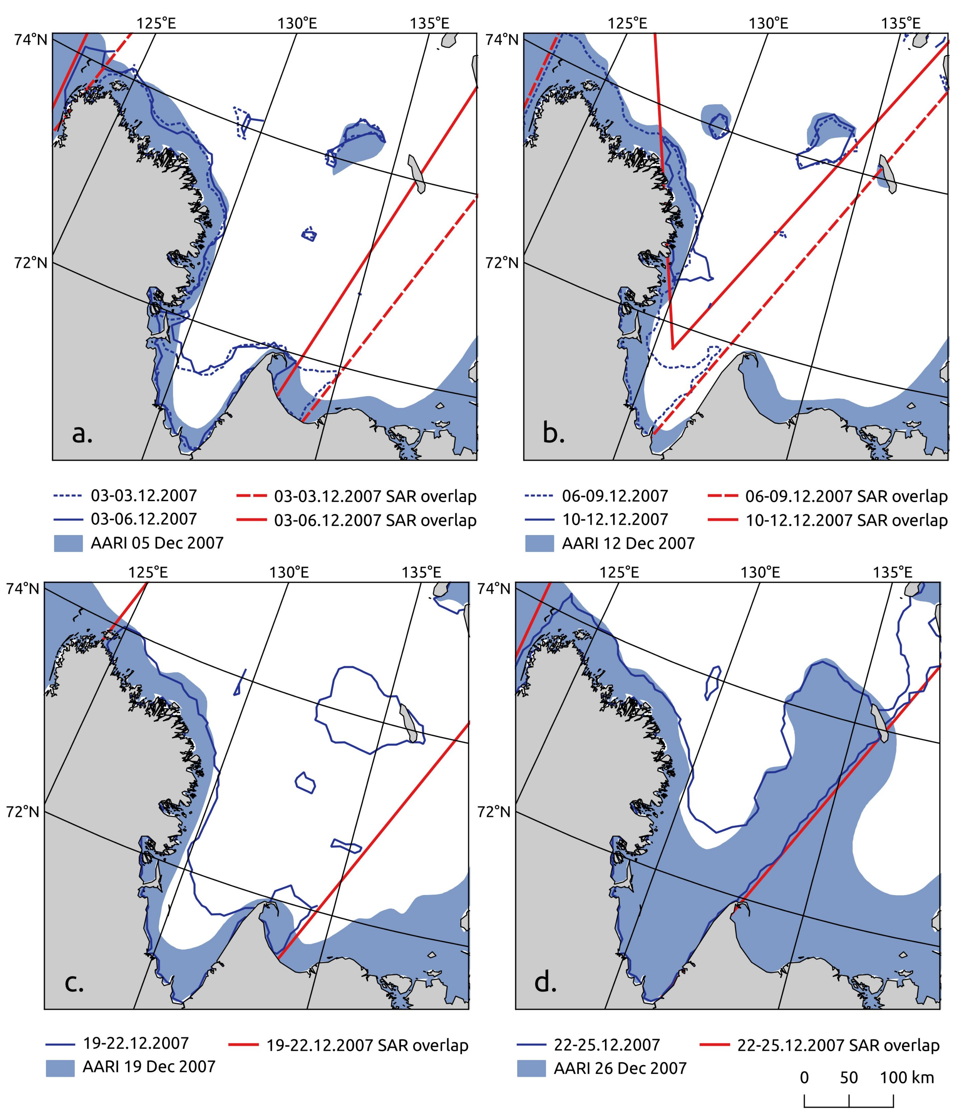
The two features located at 74 N were also present on the AARI ice charts for 5 and 12 December and disappeared on the following charts (Figure 5a,b). According to the generated data, those features existed from 3 to 22 December 2007. Another group of features, not shown in the AARI ice charts, appeared in the central part of the region between 6 and 22 December. This area corresponds to the location of shoals with a water depth of less than 20 m and is a typical location of seasonal stamukhas [6,29,30]. The detected features are likely stamukhas/groups of stamukhas. Their horizontal sizes are 10–40 km along the narrow axis. A previous study showed that similar features occur on the AARI ice charts in several seasons between 1999 and 2015 [6]. Therefore, we suggest that the features were not intentionally ignored by the sea ice experts. The relatively small horizontal size of the features or absence of visible drift motion around the feature may cause inaccuracy in regional sea ice charts produced manually.
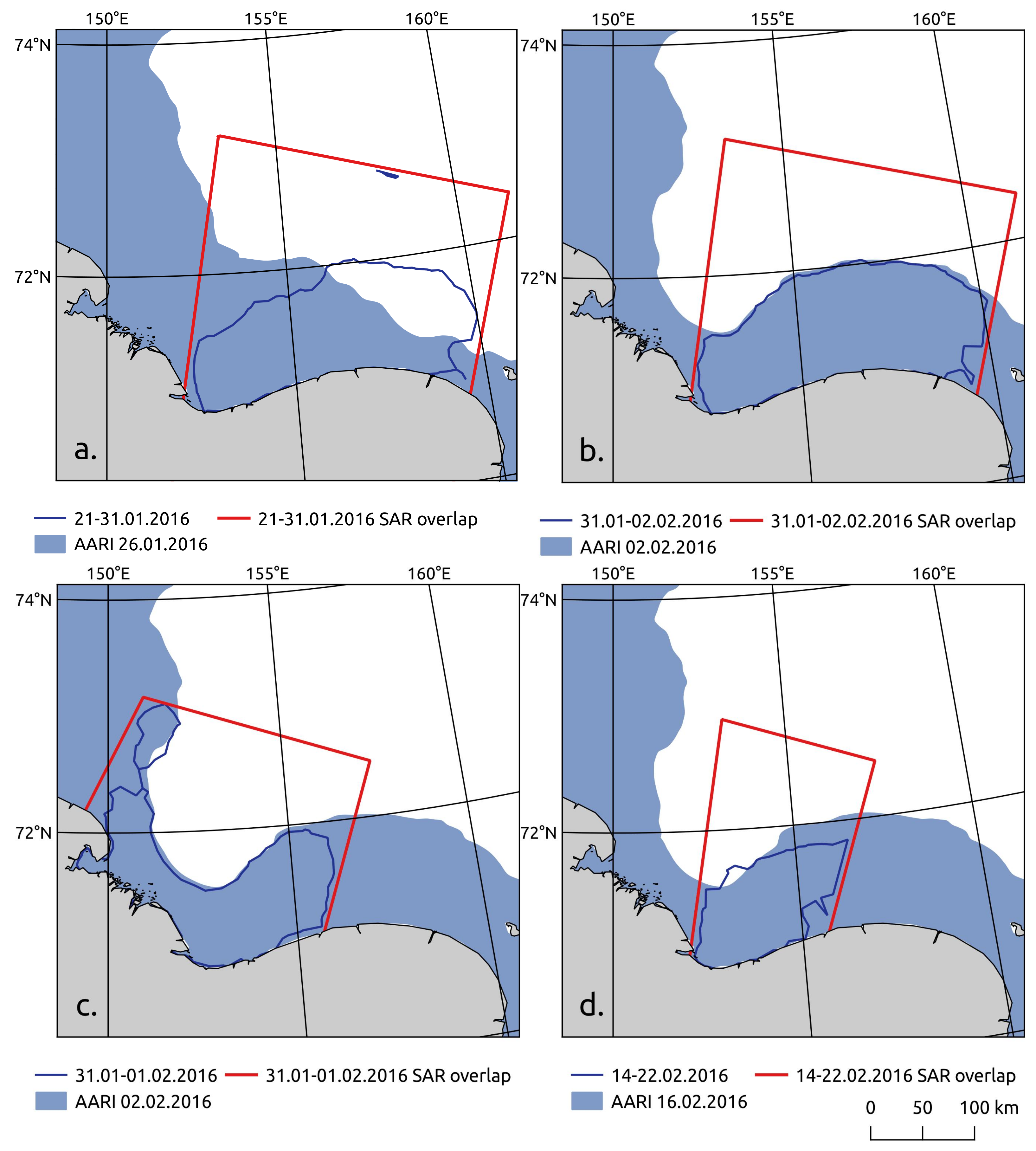
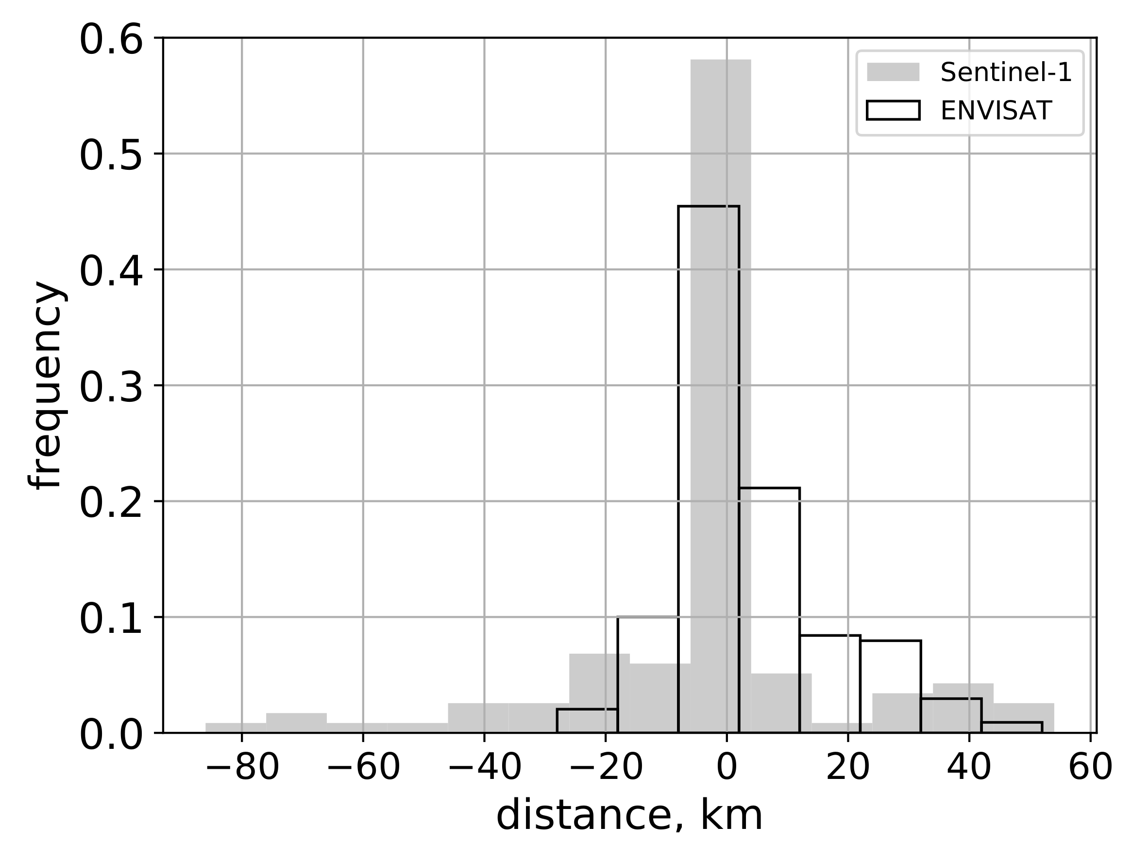
Figure 7 shows the distribution of the distances between the AARI and the derived fast ice edges. Both the ENVISAT and Sentinel-1 data show a mode near 0-value. The mean absolute distance between the resultant and the AARI fast ice edge is 9.7 km and 15.0 km for the ENVISAT and Sentinel-1 data correspondingly. The distribution modes lie between −16 and 2 km. More than 40% of the measured distances lie in this range for both data sets. For ENVISAT data, the maximal differences of tens of kilometers correspond to the cases when the method largely overestimates the fast ice conditions in the central part of the region, where the variability of the edge location is the largest [6]. This can be partly explained by the difference in the analyzed time intervals. While the sea ice expert observed the sea ice conditions for 3–5 days, the mean pairwise image time difference varied from 1 to 4 days. Even a short mismatch in the observed period may cause a difference in the edge location caused by the changes in fast ice cover. Figure 6a,b illustrates the case when a significant difference in the location of the AARI and the retrieved fast ice edge was caused by the difference in the timing of fast ice observation. The AARI chart issued on 26 January 2016 is 5 days apart from the first and the second image in the processed SAR image pair (Figure 5a). The retrieved fast ice polygon depicts a more advanced in time location of the fast ice edge which coincided with the following by date AARI ice chart (Figure 5b). Apart from the described above case, the fast ice edge derived from Sentinel-1 data fits well with the fast ice edge from AARI ice charts (Figure 5b–d) which is also confirmed by the high frequency (over 60%) of near-zero distances between the compared edges.
The accuracy of the proposed method largely depends on the resolution and quality of sea ice drift algorithm output. The drift retrieval approach used in this study was adapted to fast ice detection which allows to increase the resolution of the gridded product to the size of 10–20 pixels of the input SAR image. This potentially will allow mapping of fast ice and stamukhas at sub-kilometer scale from wide-swath SAR data. The method proposed in this study can be used in operational mode as an objective tool for fast ice mapping where performance is mainly limited by two factors: reasonable time gap between SAR images over an area of interest and presence of recognizable ice features on the images. From our test calculations, it performs well in the winter season but potential problems with ice features tracking may arise when ice is starting to melt—the SAR signature of both fast and drift ice becomes homogeneous which leads to indistinct ice surface features. In this case, optical or infrared data are more suitable. The time difference between Sentinel-1 images typically varies from 12 to 48 h in the Pechora, Kara and Laptev Seas. The Sentinel-1 constellation observation scenario shows the lowers frequencies of observations (2–4 days) over the Chukchi Sea [31], which is still suitable for applying our algorithm in the region. Therefore, the algorithm can be applied to detect fast ice and stamukhas all over the arctic coasts.
More extensive testing of the algorithm is needed with visual inspection of actual fast ice edge positions. In our study we used ice charts as reference data, in many cases the process of fast ice mapping is subjective and in most cases implies generalization—rather than accuracy. We expect that the developed method can be used as a tool to increase the quality of fast ice and stamukhas mapping.
4. Conclusions
A new automated method of fast ice detection from C-band SAR imagery was developed and tested. A comparison with the operational sea ice charts showed that the developed method is capable of accurate fast ice edge delineation and detection of large stamukhas. The mean distance between the detected fast ice edges and the corresponding manually derived ones from the operational sea ice charts is in order of 10 km. The accuracy of the method and the size of the detectable stamukhas depends on the initial image resolution and internal method parameters. In this study, stamukhas with a horizontal size of 10 km were detected. The method can be used in support of sea ice services providing near-real-time information on the location of the fast ice edge and location of stamukhas. It also can be used for fast ice and large stamukhas monitoring on a regional scale. The obtained information on fast ice edge location and presence of stamukhas can be used in interdisciplinary research of the Arctic coastal areas, particularly for coastal erosion and submarine permafrost investigation.
Author Contributions
Conceptualization, V.S., D.D.; methodology, V.S., D.D.; software, D.D., V.S.; cross-comparison, V.S.; original draft preparation, V.S., D.D. All authors have read and agreed to the published version of the manuscript.
Funding
This research was funded by RFBR, project number 19-35-60033.
Institutional Review Board Statement
Not applicable.
Informed Consent Statement
Not applicable.
Data Availability Statement
Publicly available datasets were analyzed in this study. Sentinel-1 data can be obtained free of charge from the Copernicus Open Access Hub. (https://scihub.copernicus.eu/ (accessed on 1 July 2021)) or the Alaska Satellite Facility Vertex interface. (https://vertex.daac.asf.alaska.edu/ (accessed on 1 July 2021)). The ENVISAT ASAR data can be downloaded from the EOLI-SA user interface by the European Space Agency (ESA). (https://earth.esa.int/eogateway/ (accessed on 1 July 2021)). The operational sea ice charts are available through the World Data Center for Sea Ice at the Arctic and Antarctic Research Institute. (http://wdc.aari.ru/datasets/d0004/ (accessed on 24 June 2021)). The Python and C++ code to reproduce the data set can be found here: (https://github.com/xdenisx/ice_drift_pc_ncc/releases/tag/1.0.2 (accessed on 15 September 2021)).
Acknowledgments
We thank the editor and two anonymous reviewers for their constructive comments, which helped us to improve the manuscript.
Conflicts of Interest
The authors declare no conflict of interest.
Appendix A. Displacement Threshold
Figure A1.
Algorithm sensitivity to the varying displacement threshold tested with Sentinel-1 (a–c) and ENVISAT data (d). The red lines indicate the overlap of the processed SAR images. The dashed yellow and dark blue lines show the derived fast ice polygons. The fast ice from the AARI chart is shown in light blue.

Appendix B. Algorithm Parameters
Step 1:
- Time difference between imagesThe tested time difference between images in pairs is up to 10 days. The recommended time difference is up to 20 days. Over a longer time period, the features might become unrecognizable due to evolution of the sea ice surface;
- Block sizeBlock size is the size of the rectangular container of pixels (image patch) in successive images. The recommended range of the block size is 16–64, which typically corresponds to 800–6400 ground meters for satellite SAR wide swath data. In this study, block size was set to 64;
- Search areaTo find correspondences in successive SAR images, the similarity of image patches extracted in the first image is measured by correlation analysis within a defined search window or search area in the second image. The search area is set by a factor and the block size. To reduce the computational time and detect stationary sea ice features with a near-zero drift, the factor was set to 4 (the search area equals 64 × 4 pixels);
- Grid stepThe recommended range of grid step is 20–40 pixels. Smaller grid steps can be used for the detection of stamukhas, but the computational cost will be higher.
Step 2:
- Displacement thresholdA sensitivity study showed that the best results are obtained with 120–150 m values independently from the initial image resolution (Figure A1).
Step 3:
- AlphaThe optimal alpha parameter depends on the grid step, quality of the drift data, configuration of the fast ice edge, and the vicinity of stamukhas. The recommended alpha values are in the range of 2–10 grid step. Stamukhas located within alpha distance to the fast ice edge will be included in the fast ice polygons. The smaller the alpha, the greater the number of separate polygons that are derived.
References
- Mahoney, A.; Eicken, H.; Shapiro, L.; Graves, A. Defining and locating the seaward landfast ice edge in northern Alaska. In Proceedings of the 18th International Conference on Port and Ocean Engineering under Arctic Conditions (POAC’05), Potsdam, NY, USA, 26–30 June 2005; pp. 991–1001. [Google Scholar]
- Mahoney, A.; Eicken, H.; Gaylord, A.G.; Shapiro, L. Alaska landfast sea ice: Links with bathymetry and atmospheric circulation. J. Geophys. Res.-Ocean. 2007, 112. [Google Scholar] [CrossRef] [Green Version]
- Reimnitz, E.; Dethleff, D.; Nurnberg, D. Contrasts in Arctic Shelf Sea-Ice Regimes and Some Implications—Beaufort Sea Versus Laptev Sea. Mar. Geol. 1994, 119, 215–225. [Google Scholar] [CrossRef]
- Sneed, W.A.; Hamilton, G.S. Recent changes in the Norske Øer Ice Barrier, coastal Northeast Greenland. Ann. Glaciol. 2016, 57, 47–55. [Google Scholar] [CrossRef] [Green Version]
- Zubov, N.N. Arctic Sea Ice; Izd. Glavsevmorputi: Moscow, Russia, 1945. (In Russian) [Google Scholar]
- Selyuzhenok, V.; Krumpen, T.; Mahoney, A.; Janout, M.; Gerdes, R. Seasonal and interannual variability of fast ice extent in the southeastern Laptev Sea between 1999 and 2013. J. Geophys. Res. Ocean. 2015, 120, 7791–7806. [Google Scholar] [CrossRef] [Green Version]
- Mahoney, A.; Eicken, H.; Shapiro, L. How fast is landfast sea ice? A study of the attachment and detachment of nearshore ice at Barrow, Alaska. Cold Reg. Sci. Technol. 2007, 47, 233–255. [Google Scholar] [CrossRef]
- Yu, Y.L.; Stern, H.; Fowler, C.; Fetterer, F.; Maslanik, J. Interannual Variability of Arctic Landfast Ice between 1976 and 2007. J. Clim. 2014, 27, 227–243. [Google Scholar] [CrossRef]
- Eicken, H.; Dmitrenko, I.; Tyshko, K.; Darovskikh, A.; Dierking, W.; Blahak, U.; Groves, J.; Kassens, H. Zonation of the Laptev Sea landfast ice cover and its importance in a frozen estuary. Glob. Planet. Chang. 2005, 48, 55–83. [Google Scholar] [CrossRef]
- Wegner, C.; Wittbrodt, K.; Hölemann, J.; Janout, M.; Krumpen, T.; Selyuzhenok, V.; Novikhin, A.; Polyakova, Y.; Krykova, I.; Kassens, H.; et al. Sediment entrainment into sea ice and transport in the Transpolar Drift: A case study from the Laptev Sea in winter 2011/2012. Cont. Shelf Res. 2017, 141, 1–10. [Google Scholar] [CrossRef] [Green Version]
- Overeem, I.; Anderson, R.S.; Wobus, C.W.; Clow, G.D.; Urban, F.E.; Matell, N. Sea ice loss enhances wave action at the Arctic coast. Geophys. Res. Lett. 2011, 38. [Google Scholar] [CrossRef]
- Shabanova, N.; Ogorodov, S.; Shabanov, P.; Baranskaya, A. Hydrometeorological forcing of western Russian Arctic coastal dynamics: XX-century history and current state. Geogr. Environ. Sustain. 2018, 11, 113–129. [Google Scholar] [CrossRef] [Green Version]
- Ogorodov, S.; Kamalov, A.; Zubakin, G.; Gudoshnikov, Y.P. The role of sea ice in coastal and bottom dynamics in the Pechora Sea. Geo-Mar. Lett. 2005, 25, 146–152. [Google Scholar] [CrossRef]
- Ogorodov, S.; Aleksyutina, D.; Baranskaya, A.; Shabanova, N.; Shilova, O. Coastal Erosion of the Russian Arctic: An Overview. J. Coast. Res. 2020, 95, 599–604. [Google Scholar] [CrossRef]
- Ogorodov, S.; Arkhipov, V.; Baranskaya, A.; Kokin, O.; Romanov, A. The influence of climate change on the intensity of ice gouging of the bottom by hummocky formations. In Doklady Earth Sciences; Springer: Berlin, Germany, 2018; Volume 478, pp. 228–231. [Google Scholar]
- Fraser, A.D.; Massom, R.A.; Michael, K.J. A Method for Compositing Polar MODIS Satellite Images to Remove Cloud Cover for Landfast Sea-Ice Detection. IEEE Trans. Geosci. Remote Sens. 2009, 47, 3272–3282. [Google Scholar] [CrossRef]
- Meyer, F.J.; Mahoney, A.R.; Eicken, H.; Denny, C.L.; Druckenmiller, H.C.; Hendricks, S. Mapping arctic landfast ice extent using L-band synthetic aperture radar interferometry. Remote Sens. Environ. 2011, 115, 3029–3043. [Google Scholar] [CrossRef]
- Karvonen, J. Estimation of Arctic land-fast ice cover based on dual-polarized Sentinel-1 SAR imagery. Cryosphere 2018, 12, 2595–2607. [Google Scholar] [CrossRef] [Green Version]
- Dammann, D.O.; Eriksson, L.E.; Mahoney, A.R.; Eicken, H.; Meyer, F.J. Mapping pan-Arctic landfast sea ice stability using Sentinel-1 interferometry. Cryosphere 2019, 13, 557–577. [Google Scholar] [CrossRef] [Green Version]
- Fraser, A.D.; Massom, R.A.; Ohshima, K.I.; Willmes, S.; Kappes, P.J.; Cartwright, J.; Porter-Smith, R. High-resolution mapping of circum-Antarctic landfast sea ice distribution, 2000–2018. Earth Syst. Sci. Data 2020, 12, 2987–2999. [Google Scholar] [CrossRef]
- Li, X.; Shokr, M.; Hui, F.; Chi, Z.; Heil, P.; Chen, Z.; Yu, Y.; Zhai, M.; Cheng, X. The spatio-temporal patterns of landfast ice in Antarctica during 2006–2011 and 2016–2017 using high-resolution SAR imagery. Remote Sens. Environ. 2020, 242, 111736. [Google Scholar] [CrossRef]
- Kim, M.; Kim, H.C.; Im, J.; Lee, S.; Han, H. Object-based landfast sea ice detection over West Antarctica using time series ALOS PALSAR data. Remote Sens. Environ. 2020, 242, 111782. [Google Scholar] [CrossRef]
- Giles, A.B.; Massom, R.A.; Lytle, V.I. Fast-ice distribution in East Antarctica during 1997 and 1999 determined using RADARSAT data. J. Geophys. Res.-Ocean. 2008, 113. [Google Scholar] [CrossRef] [Green Version]
- Griebel, J.; Dierking, W. Impact of sea ice drift retrieval errors, discretization and grid type on calculations of ice deformation. Remote Sens. 2018, 10, 393. [Google Scholar] [CrossRef] [Green Version]
- Demchev, D.; Volkov, V.; Kazakov, E.; Alcantarilla, P.F.; Sandven, S.; Khmeleva, V. Sea Ice Drift Tracking From Sequential SAR Images Using Accelerated-KAZE Features. IEEE Trans. Geosci. Remote Sens. 2017, 55, 5174–5184. [Google Scholar] [CrossRef]
- Demchev, D.; Eriksson, L.; Smolanitsky, V. SAR Image Texture Entropy Analysis for Applicability Assessment of Area-Based and Feature-Based Aea Ice Tracking Approaches. In Proceedings of the 13th European Conference on Synthetic Aperture Radar, VDE (EUSAR 2021), Virtual Conference. 29 March–1 April 2021; pp. 1–3. [Google Scholar]
- Lewis, J. Fast normalized cross-correlation, 1995. Vis. Interface 2010, 2010, 120–123. [Google Scholar]
- Da, T.K.F. 2D Alpha Shapes. CGAL User and Reference Manual; CGAL Editorial Board, 2015, 4.7-4 ed. Available online: hhttp://doc.cgal.org/4.7/Manual/packages.htmlPkgAlphaShape2Summary (accessed on 15 September 2021).
- Gorbunov, J.A.; Losev, S.M.; Dyment, L.N. Stamuhi morja Laptevyh (Stamukhas of the Laptev Sea). Probl. Arctiki I Antarct. 2008, 79, 111–116. [Google Scholar]
- Selyuzhenok, V.; Mahoney, A.; Krumpen, T.; Castellani, G.; Gerdes, R. Mechanisms of fast-ice development in the south-eastern Laptev Sea: A case study for winter of 2007/08 and 2009/10. Polar Res. 2017, 36, 1411140. [Google Scholar] [CrossRef] [Green Version]
- ESA. Sentinel Online. 2021. Available online: https://sentinels.copernicus.eu/web/sentinel/missions/sentinel-1/observation-scenario (accessed on 9 September 2021).
Figure 1.
Flowchart of the fast ice detection algorithm.

Figure 2.
A guide vector by the feature tracking algorithm (solid black arrow) and an associated search area W defined around the end of the vector (dotted black line). The size of searching zone W is set empirically and is 32 × 32 pixels. The red arrows illustrate potential ice drift vectors for a closest computational grid cell (red circle) by the pattern matching algorithm. The black outlined circles correspond to computational grid points used in the pattern matching algorithm.

Figure 3.
An example of methods steps output. The yellow arrows show the sea ice drift field calculated from the ENVISAT SAR image pair taken on 19 (the background image) and 22 December 2007 (step 1). The filtered near-zero displacement points are shown in red (step 2). The blue line shows the resultant fast ice polygons (step 3).

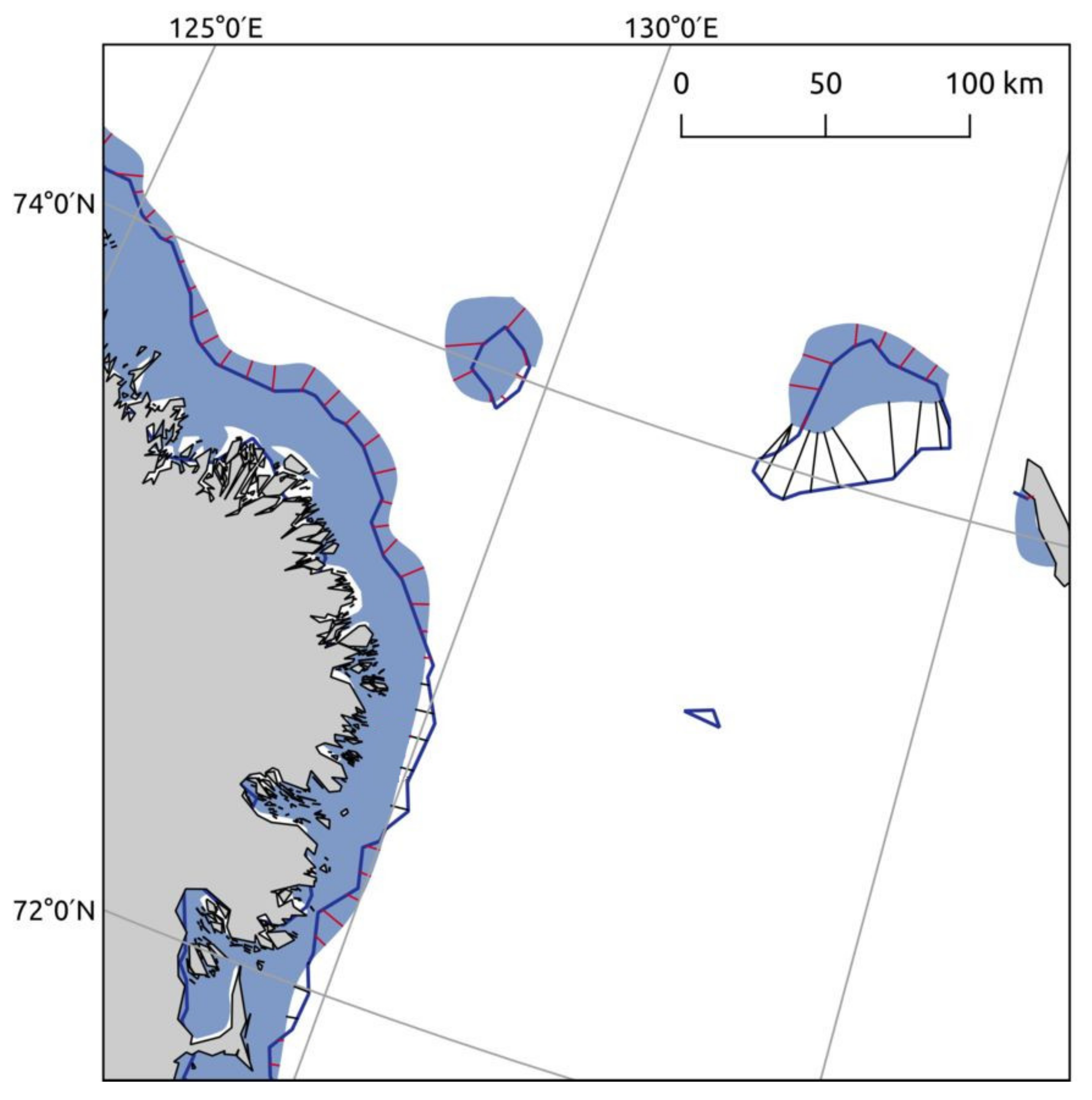
Figure 4.
The fast ice conditions near the Lena Delta for 06 December 2007. The dark blue line shows the fast ice detected by the proposed algorithm. The light blue corresponds to the fast ice from AARI map issued on 5 December 2007. For the cross-comparison, distances between the fast ice edges were measured along the black/red lines (automatically drawn Euclidean distances). The red lines correspond to the negative distances, while the black lines—to the positive ones.

Figure 5.
The retrieved ENVISAT-based fast ice polygons and the corresponding AARI fast ice data for the Laptev Sea region for 3–6 Demember 2007 (a), 6–12 December 2007 (b), 19–22 December 2007 (c), 22–26 December 2007 (d). The dates in the legend correspond to the timing of the first and the second SAR images and the issue date of the AARI ice charts.

Figure 6.
The fast ice polygons derived from Sentinel-1 data and the corresponding AARI fast ice zones over the East Siberian Sea region for 21–31 January 2016 (a), 31 January–2 February 2016 (b), 31 January–1 February 2016 (c), 14–22 February 2016 (d). The dates in the legend correspond to the timing of the first and second SAR images and the issue date of the AARI ice charts.

Figure 7.
The distribution of the measured distances between the AARI and the SAR-derived fast ice edge from ENVISAT ASAR and Sentinel-1 data. The positive values correspond to the cases when the AARI edge is closer to the shore compared to the retrieved edge. Negative values correspond to the cases when the ice edge by the AARI experts is more advanced compared to the retrieved one.


Table 1.
Cross-comparison data and results.
| Laptev Sea | East Siberian Sea | |
|---|---|---|
| Data | ENVISAT ASAR WS | S1 EWS |
| Spatial resolution | 150 m | 40 m |
| Period | 3–25 December 2007 | 21 January–22 February 2016 |
| Number of image pairs | 7 | 4 |
| Time difference between images in pairs | 0–3 days | 3–10 days |
| Total length of fast ice edge | 4400 km | 1190 km |
| Time difference between image 2 in pair and date of AARI chart issue | 0–3 days | 1–5 days |
| Abs. mean distance to AARI fast ice edge | 9.7 km | 15.0 km |
Publisher’s Note: MDPI stays neutral with regard to jurisdictional claims in published maps and institutional affiliations. |
© 2021 by the authors. Licensee MDPI, Basel, Switzerland. This article is an open access article distributed under the terms and conditions of the Creative Commons Attribution (CC BY) license (https://creativecommons.org/licenses/by/4.0/).
Share and Cite
MDPI and ACS Style
Selyuzhenok, V.; Demchev, D. An Application of Sea Ice Tracking Algorithm for Fast Ice and Stamukhas Detection in the Arctic. Remote Sens. 2021, 13, 3783. https://0-doi-org.brum.beds.ac.uk/10.3390/rs13183783
AMA Style
Selyuzhenok V, Demchev D. An Application of Sea Ice Tracking Algorithm for Fast Ice and Stamukhas Detection in the Arctic. Remote Sensing. 2021; 13(18):3783. https://0-doi-org.brum.beds.ac.uk/10.3390/rs13183783
Chicago/Turabian StyleSelyuzhenok, Valeria, and Denis Demchev. 2021. "An Application of Sea Ice Tracking Algorithm for Fast Ice and Stamukhas Detection in the Arctic" Remote Sensing 13, no. 18: 3783. https://0-doi-org.brum.beds.ac.uk/10.3390/rs13183783
Note that from the first issue of 2016, this journal uses article numbers instead of page numbers. See further details here.