
Reconstructing Ocean Heat Content for Revisiting Global Ocean Warming from Remote Sensing Perspectives


Key Laboratory of Spatial Data Mining and Information Sharing of Ministry of Education, National & Local Joint Engineering Research Center of Satellite Geospatial Information Technology, Fuzhou University, Fuzhou 350108, China
*
Author to whom correspondence should be addressed.
Remote Sens. 2021, 13(19), 3799; https://0-doi-org.brum.beds.ac.uk/10.3390/rs13193799
Submission received: 4 July 2021
/
Revised: 6 September 2021
/
Accepted: 18 September 2021
/
Published: 22 September 2021
(This article belongs to the Special Issue Deep Ocean Remote Sensing and Its Application in the Ocean Warming Study in Recent Decades)
Abstract
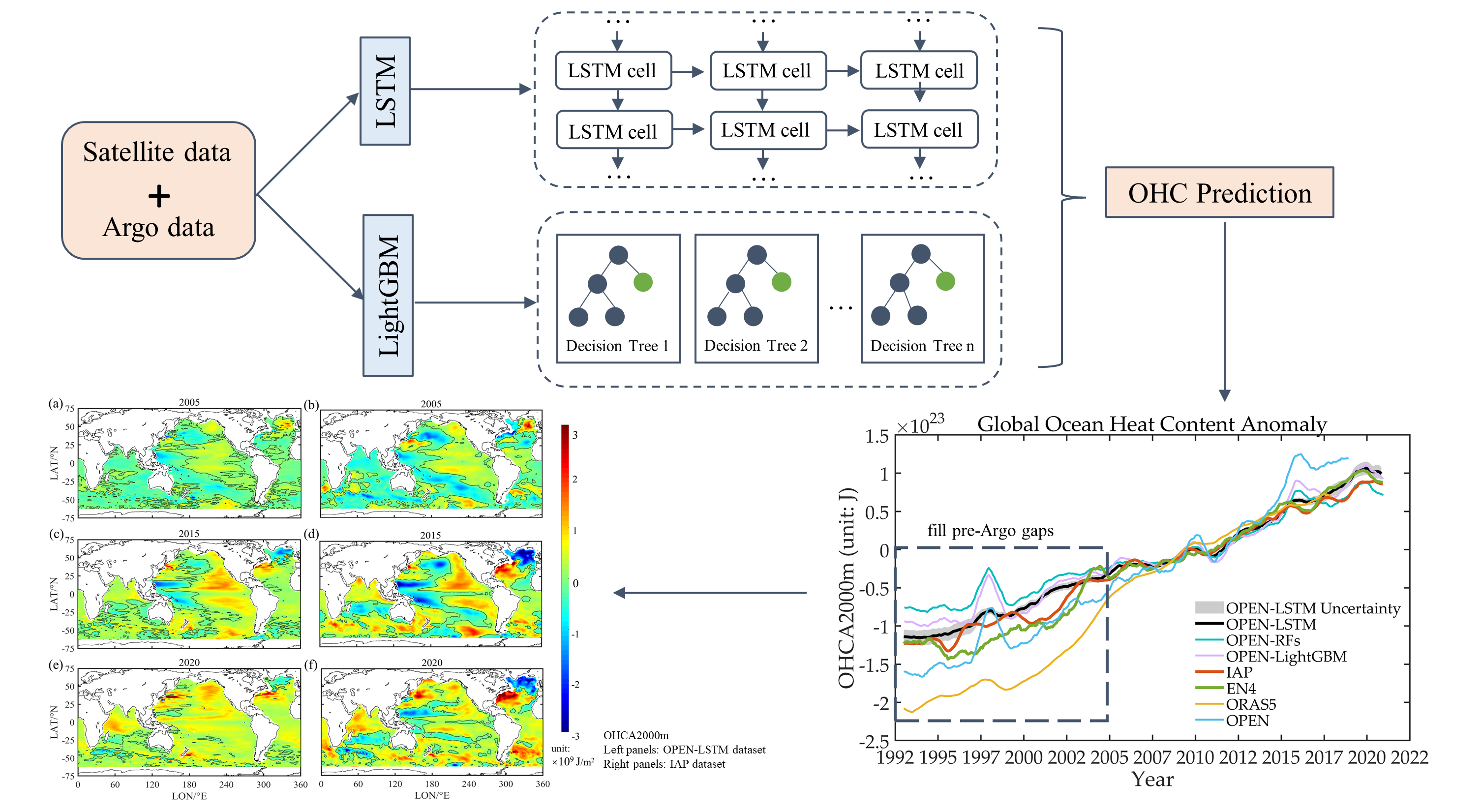
:Global ocean heat content (OHC) is generally estimated using gridded, model and reanalysis data; its change is crucial to understanding climate anomalies and ocean warming phenomena. However, Argo gridded data have short temporal coverage (from 2005 to the present), inhibiting understanding of long-term OHC variabilities at decadal to multidecadal scales. In this study, we utilized multisource remote sensing and Argo gridded data based on the long short-term memory (LSTM) neural network method, which considers long temporal dependence to reconstruct a new long time-series OHC dataset (1993–2020) and fill the pre-Argo data gaps. Moreover, we adopted a new machine learning method, i.e., the Light Gradient Boosting Machine (LightGBM), and applied the well-known Random Forests (RFs) method for comparison. The model performance was measured using determination coefficients (R2) and root-mean-square error (RMSE). The results showed that LSTM can effectively improve the OHC prediction accuracy compared with the LightGBM and RFs methods, especially in long-term and deep-sea predictions. The LSTM-estimated result also outperformed the Ocean Projection and Extension neural Network (OPEN) dataset, with an R2 of 0.9590 and an RMSE of 4.45 × 10¹⁹ in general in the upper 2000 m for 28 years (1993–2020). The new reconstructed dataset (named OPEN-LSTM) correlated reasonably well with other validated products, showing consistency with similar time-series trends and spatial patterns. The spatiotemporal error distribution between the OPEN-LSTM and IAP datasets was smaller on the global scale, especially in the Atlantic, Southern and Pacific Oceans. The relative error for OPEN-LSTM was the smallest for all ocean basins compared with Argo gridded data. The average global warming trends are 3.26 × 10⁸ J/m2/decade for the pre-Argo (1993–2004) period and 2.67 × 10⁸ J/m2/decade for the time-series (1993–2020) period. This study demonstrates the advantages of LSTM in the time-series reconstruction of OHC, and provides a new dataset for a deeper understanding of ocean and climate events.

1. Introduction
Recently, atmospheric greenhouse gases (GHGs) have caused imbalances in the top layers of the atmosphere, giving rise to the Earth’s energy imbalance (EEI) which is ultimately driving the current warming trend [1,2,3]. Darrell et al. [4] found that global warming in the past 150 years has far exceeded what occurred in the last 6000 years. Increasing global warming has led to the destabilization of the climate system and caused more frequent and severe extreme climate events. For example, the strong El Niños during 2014–2016, 2017, 2018, and 2019 reached the highest warmth in the upper ocean in modern recorded history [5,6,7], and upper ocean temperatures hit a record high in 2020 [8]. Behind these anomalous incidents, the ocean plays an essential role in regulating the global climate system and redistributing regional and global-scale energy.
Indeed, the ocean is constantly warming in its interior [9,10,11]. More and more studies have shown that the ocean absorbs most of the EEI (up to 93.4%) in the form of heat, which gradually warms the ocean (300–2000 m) [12,13,14,15]. Cheng et al. [16] found that the ocean absorbs energy at accelerating rates and that the deep ocean (700–2000 m) plays an increasingly important role. Recent studies have also shown that warming signals have been detected in the ocean below 2000 m, especially in the Southern Ocean [17]. Therefore, studying ocean transfer at different depth ranges is essential because of the global warming crisis brought about by the EEI and the dominant heat capacity of the ocean. Thus, the ocean is an integral part of the heat cycle and an important regulator of the climate system.
At the same time, ocean heat content (OHC) is an essential parameter characterizing the ocean thermal state and an efficient parameter by which to evaluate the EEI [18,19]. Many studies have shown that OHC is related to some climate events and natural internal climate variabilities (e.g., the South China Sea summer monsoon intensity, tropical cyclone intensity, Interdecadal Pacific Oscillation, Atlantic Multidecadal Oscillation, El Niño–Southern Oscillation (ENSO), and Indian Ocean Dipole [IOD]) [20,21,22,23]. Therefore, estimating OHC and monitoring its long-term change is greatly significant in analyzing air–sea interactions and natural variabilities on decadal to multidecadal scales.
The modes of ocean observation have been improving for a long time [24]; for example, the introduction of Argo buoys reduced the standard deviation caused by incomplete samples to the lowest value [25]. The Argo observation network was established in 2005, and although its floats number around 4000 globally, meeting the needs of long-term and large-scale research is still difficult. For the pre-Argo period, the ocean observation system was mainly based on expendable bathythermograph (XBT) and mechanical bathythermograph (MBT) conventional floats, giving rise to uncertainties and discrepancies in measurements. Boyer et al. [26] pointed out that the uncertainties in OHC estimates are due to instrument biases (especially for XBT bias), mapping methods, and definitions of baseline climatology. The uncertainty in the measured data in the pre-Argo period and the short temporal coverage in the Argo period bring certain difficulties with regard to global heat estimations.
However, space-to-Earth observation systems have, in the meantime, become the most important source of observational data, and play an irreplaceable role in marine scientific research. Large-scale remote sensing data with high temporal and spatial resolutions can be used to obtain sea surface information. As sea surface features can reflect the dynamic phenomena within the ocean, these systems may be used to derive internal information represented on the sea surface [27]. Therefore, combining Argo gridded data and remote sensing data is an effective way of determining long-term and large-scale three-dimensional thermohaline structures in the ocean.
Various thermohaline structure reconstruction methods using satellite data are proposed: the dynamic, empirical methods, numerical assimilation, and statistical methods. First, in the dynamic method, some complex dynamic processes are ignored because of theoretical simplifications. Therefore, block modeling is applied, that is, the internal plus surface quasi-geostrophic method (iSQG), when applied on a global scale [28]. Second, the empirical method uses ocean hydroacoustic data to expand the scope of available observational data [29]. Thus, it is more suitable for areas with sufficient observations. Third, numerical assimilation is an essential tool for generating reanalysis datasets. For example, current, well-known datasets such as the European Centre for Medium-Range Weather Forecasts (ECWMF) Ocean Reanalysis System 5 (ORAS5) and Simple Ocean Data Assimilation (SODA) datasets are derived using this method [30,31]. Finally, statistical methods are the most widely used, especially with the development of high-efficiency neural networks, and they usually achieve good performance.
Crucial thermohaline information retrieval methods based on artificial intelligence (AI)/machine learning have been developed using support vector machines, random forests (RFs), and extreme gradient boosting (XGBoost) [32,33,34]. It is worth noting that a geographically weighted regression model considering spatial nonstationary features in the ocean has a low root-mean-square error (RMSE) [35]. Lu et al. [36] proposed a new method which combines a preclustering process and an artificial neural network (ANN); its results were better than those of traditional methods and the clustering or ANN method exclusively. However, with global warming, these methods must not be limited to monitoring sea surface temperature (SST) and other thermohaline information.
Chacko et al. and Jagadeesh et al. [37,38] used an ANN to retrieve OHC in the north Indian Ocean. Irrgang et al. [39] estimated global OHC from 1990–2015 from tidal magnetic satellite observations using an ANN algorithm. Su et al. [40] used an ANN to construct a long-term OHC dataset, known as the Ocean Projection and Extension neural Network (OPEN), which shows a comparative advantage with the IAP dataset. However, these methods lack temporal dependence considerations. Some scholars have used recurrent neural networks (RNNs) and long short-term memory (LSTM) to inverse SST, sea surface height anomaly (SSHA) [41,42,43,44], and so on. However, these have not been fully applied to OHC retrieval, especially for long-term reconstruction.
Thus, this study used LSTM to improve the accuracy of OHC prediction by considering the temporal dependence of oceanic variables. Based on satellite data with space-time parameters (longitude [LON], latitude [LAT], day of year [DOY]) and Argo data, we reconstructed the OHC dataset for an extended period (1993–2020), filling in gaps in the pre-Argo period. This study compared the advantages of LSTM over Light Gradient Boosting Machine (LightGBM) and RFs for OHC time-series estimation, and then evaluated the accuracy of the constructed OHC datasets. Finally, the new datasets were employed in a global ocean warming study.
2. Study Area and Data
In this study, we selected the global ocean (180° W to 180° E, 78.375° S to 77.625° N) as our study area. The multisource satellite and Argo gridded data used in this study are as follows (Table 1):
- (1)
- sea surface temperature (SST), acquired from the Optimum Interpolation Sea Surface Temperature (OISST) product, constructed by combining data from the Advanced Very High-Resolution Radiometer satellite and other observations datasets since 1981, with a spatial resolution of 0.25° × 0.25°;
- (2)
- sea surface height (SSH), observed from the Absolute Dynamic Topography products of Archiving, Validation, and Interpretation of Satellite Oceanographic (AVISO) altimetry project since 1993, with a spatial resolution of 0.25° × 0.25°;
- (3)
- sea surface wind (SSW), provided by the Cross-Calibrated Multi-Platform (CCMP) wind velocity data from the National Center for Atmospheric Research since 1987, with a spatial resolution of 0.25° × 0.25°;
- (4)
- Argo, gridded data including 27 standard horizons in the upper 2000 m since 2005, with a spatial resolution of 1° × 1°.
The comparison and verification datasets used in this study are as follows (Table 1):
- (1)
- EN4, version 4.2.1 from the Hadley Met Office of the United Kingdom, which applied objective analysis from observation datasets (e.g., WOD and Argo) since 1900, 1° × 1° [45];
- (2)
- IAP, from the Institute of Atmospheric Physics of China, which used Ensemble Optimal Interpolation (En-OI) mapping, combined with Coupled Model Intercomparison Project Phase 5 (CMIP5) multimodel datasets since 1940, 1° × 1° [16];
- (3)
- ORAS5, from the ECMWF, which assimilated various observational data in an ocean model since 1979, 1° × 1° [30];
- (4)
- OPEN, from Fuzhou University, which used remote sensing data and an ANN machine learning method to achieve temporal hindcast and provided a continuous record of the global ocean since 1993, 1° × 1° [40].
Based on previous studies, this study used seven independent variables to estimate OHC, including remote sensing data and space–time parameters (i.e., SST, SSH, USSW, VSSW [u and v components of SSW], LON, LAT, and DOY). It is likely not necessary to consider sea surface salinity in large-scale and time series variations [40,46]. The spatial resolution of sea surface data was unified to 1° × 1° by the nearest neighbor interpolation method, and the temporal resolution was unified monthly. The dataset range was normalized to [−1, 1]. Data normalization can avoid errors and further improve the performance of the model.
In this study, the OHC calculated depths were 100, 300, 700, 1000, 1500, and 2000 m, denoted as OHC100 m, OHC300 m, and so on. The climatology used in this study for OHC anomaly (OHCA) was a common baseline period from 2005 to 2014. All OHCA time-series used a 12-month running mean.
The calculation formula for the OHC (unit: J/m2) of each grid point is as follows:
where is the thermal capacity, which is constant at 3850 J kg−10 C−1; is the constant density equal to 1025 kg m−3; T is the temperature; and z is the current calculated ocean depth.
3. Methods
3.1. LSTM
LSTM is a special type of RNN proposed by Hochreiter and Schmidhuber in 1997 [47,48]. RNN can only learn short-term time dependence, essentially because it is prone to gradient decay or eventual degradation of the values passed from layer to layer. However, LSTM uses gating algorithms, i.e., an input gate, forget gate, and output gate, which can resolve the vanishing and exploding gradient problem of RNN by controlling long-distance dependence and selectively forgetting data to prevent information overload. To date, LSTM has achieved remarkable results in translation, recognition, video, and marine applications (e.g., predicting El Niño changes) [49].
LSTM adds the cell state to the hidden state based on the RNN; controls information that selectively passes through the gates. The LSTM network can be formulated as follows:
where , and are the outputs of the nonlinear activation function sigmoid functions σ, whose values (0 and 1) indicate whether information should be passed or not (0 means not allowed to pass; 1 means completely passed); and are the weight matrices of the current time; is the original input; is the output value at the last time; is the bias vector; and represent the internal status update; is the output of the LSTM cell at the current moment; and represents the multiplication of the corresponding elements of the matrix.
The ocean data presents inherent spatial nonlinearity and temporal dependence features, and the OHC is a temporally autocorrelated variable. Hence, the LSTM model, which has the ability to grasp these features, was used to reconstruct the dataset.
3.2. LightGBM
The Light Gradient Boosting Machine (LightGBM) was proposed by Microsoft Research Asia in 2017 on the basis of the gradient-boosted decision tree (GBDT) model [50]. It introduces a leaf-wise strategy with depth constraint rather than a level-wise strategy for GBDT in decision tree growth. In addition, LightGBM adopts a histogram algorithm which transforms traversal histograms, as opposed to traversal samples, in order to reduce complexity. Moreover, the strategy of gradient-based, one-side sampling and exclusive feature bundling can efficiently reduce the number of required calculations. The model supports parallel learning, which can optimize training speed and economize storage space.
LightGBM is an advanced ensemble learning algorithm which has the characteristics of less training time and high accuracy, and can provide better solutions than other classic machine learning methods. As such, this study used it as a comparison of LSTM to estimate OHC.
3.3. RFs
RFs is a well-known ensemble learning algorithm based on the bagging strategy, which takes a decision tree as the base learner [51]. A decision tree is constructed using the samples taken each time, with each decision tree having the same weight. This study used this widely-used, classic method as a comparison for OHC reconstruction.
3.4. Experimental Design
The experimental design for three models mainly includes model training, remote sensing inversion, and time-series reconstruction. We selected remote sensing data and Argo gridded data from 2005 to 2014 (120 months) as the training dataset and from 2016 to 2018 (36 months) as the validation dataset. We established the relationship model between the sea surface and subsurface after tuning the hyperparameters. Then, we reconstructed longtime-series OHC datasets. The Argo, EN4, IAP, ORAS5, and OPEN datasets were used to evaluate the accuracy (determination coefficient (R2), the root-mean-square error (RMSE), and relative error in the results in this study.
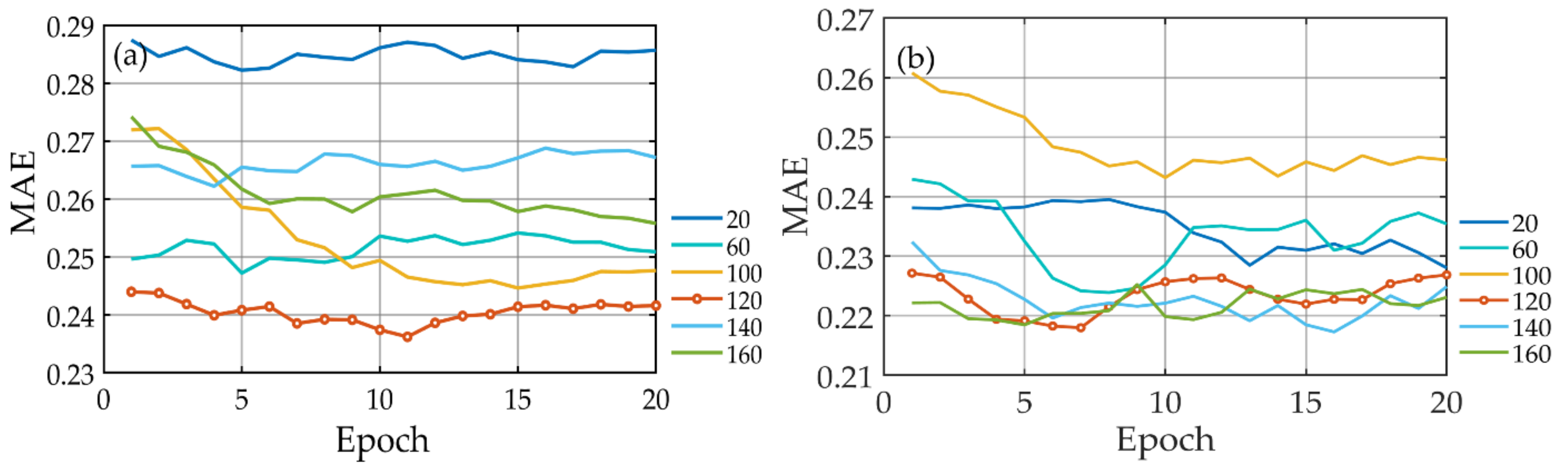
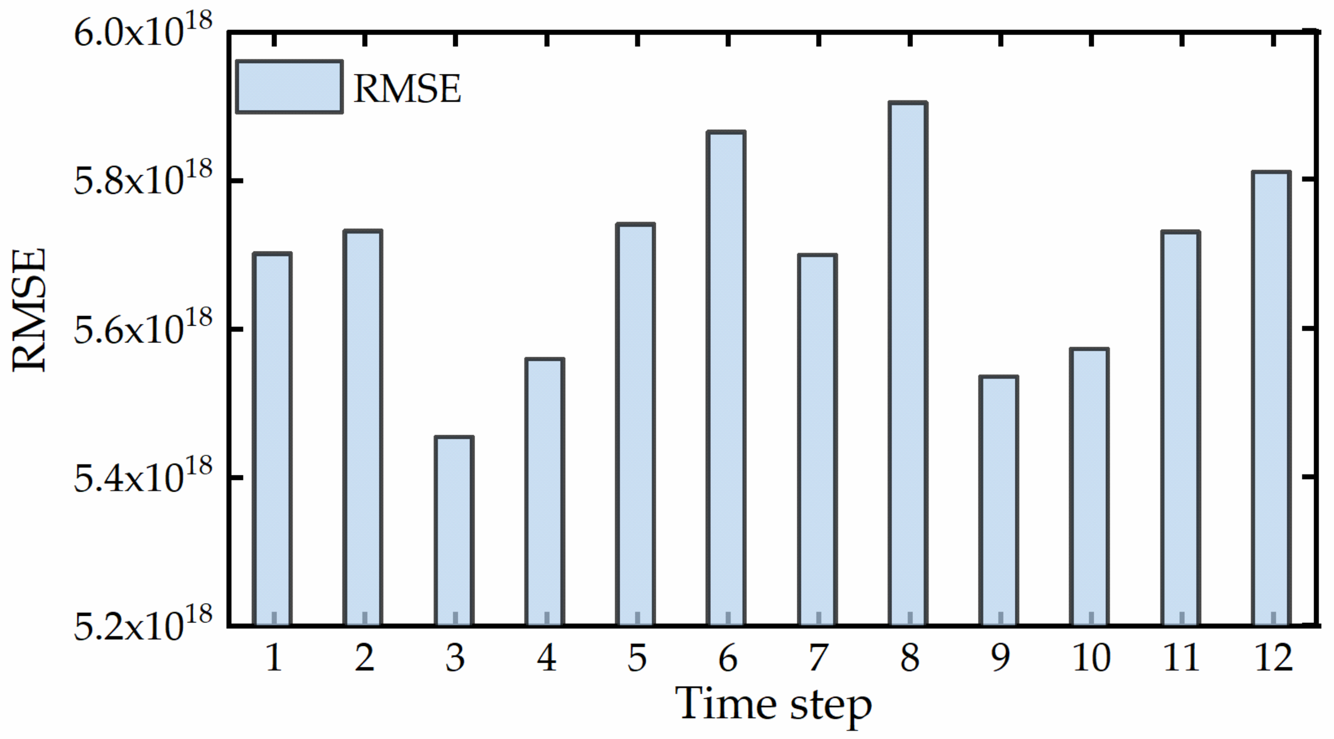
This study expects that LSTM will achieve good reconstruction performance. So, the model requires that the hyperparameters be determined, i.e., the number of layers, hidden units, iterations, and time steps. The mean absolute error (MAE) is used as the loss function, the adaptive moment estimation (Adam) is used as the optimizer, and the rectified linear unit (ReLU) is used as the activation function of all layers. The MAE changes of the experimental hyperparameters are partly shown in Figure 1 and Figure 2. When there is only one LSTM layer, the MAE first decreases and then increases as the number of hidden neurons increases. When the number of hidden neurons is set to 120, the model error is the lowest, and the average value is 0.2407. Upon adding another layer, the MAE changes within a small range but gradually stabilizes. Considering the model performance and fitting effect, the number of hidden neurons of the two layers is set to 120, and the average error of the model is the lowest (0.2235). This study tests the time step in the range of 1–12 months. The results show that when the time step is 3, the model error, i.e., RMSE, is the lowest, followed by those at time steps 9, 10, and 4. The worst accuracy is that for time step 8. The model has the best performance and greatest robustness when the time step is 3.
After a series of experiments, we determined that the model in this study must have four layers: the input layer, two LSTM layers, and a dense layer. The two LSTM layers both contain 120 hidden neurons; the epoch parameter is set to 40, and the time step for predicting OHC300 m is set to 3. The dropout rate used in each layer is set to 0.3 to prevent overfitting. The optimal model parameters are shown in Table 2.
The values of the above parameters may not be optimal, but considering the loss function and accuracy evaluation, the model’s prediction result is within an acceptable range. For predictions at different depth ranges, the parameters were adjusted appropriately; that is, for LSTM, the time steps were set to 2 for 0–100 m, 3 for 0–300 m, 6 for 0–700 m, 4 for 0–1000 m, 5 for 0–1500 m, and 5 for 0–2000 m.
For LightGBM, there are three important parameters: n_estimators (the number of residual trees), learning_rate, num_leaves (control the number of leaf nodes). The performance is well optimized with n_estimators = 1200; learning_rate = 0.1; and num_leaves = 80. Currently, the model’s error is the lowest, and its prediction ability is stable (RMSE = 6.01 × 10¹⁸ J). For RFs, there are two important parameters: ntree (the number of decision trees in the model), and mtry (the number of features contained in each decision tree). The performance of the RFs model is well optimized with ntree = 300 and mtry = 6 (RMSE = 5.97 × 10¹⁸ J).
4. Results and Discussion
4.1. Monotemporal Prediction
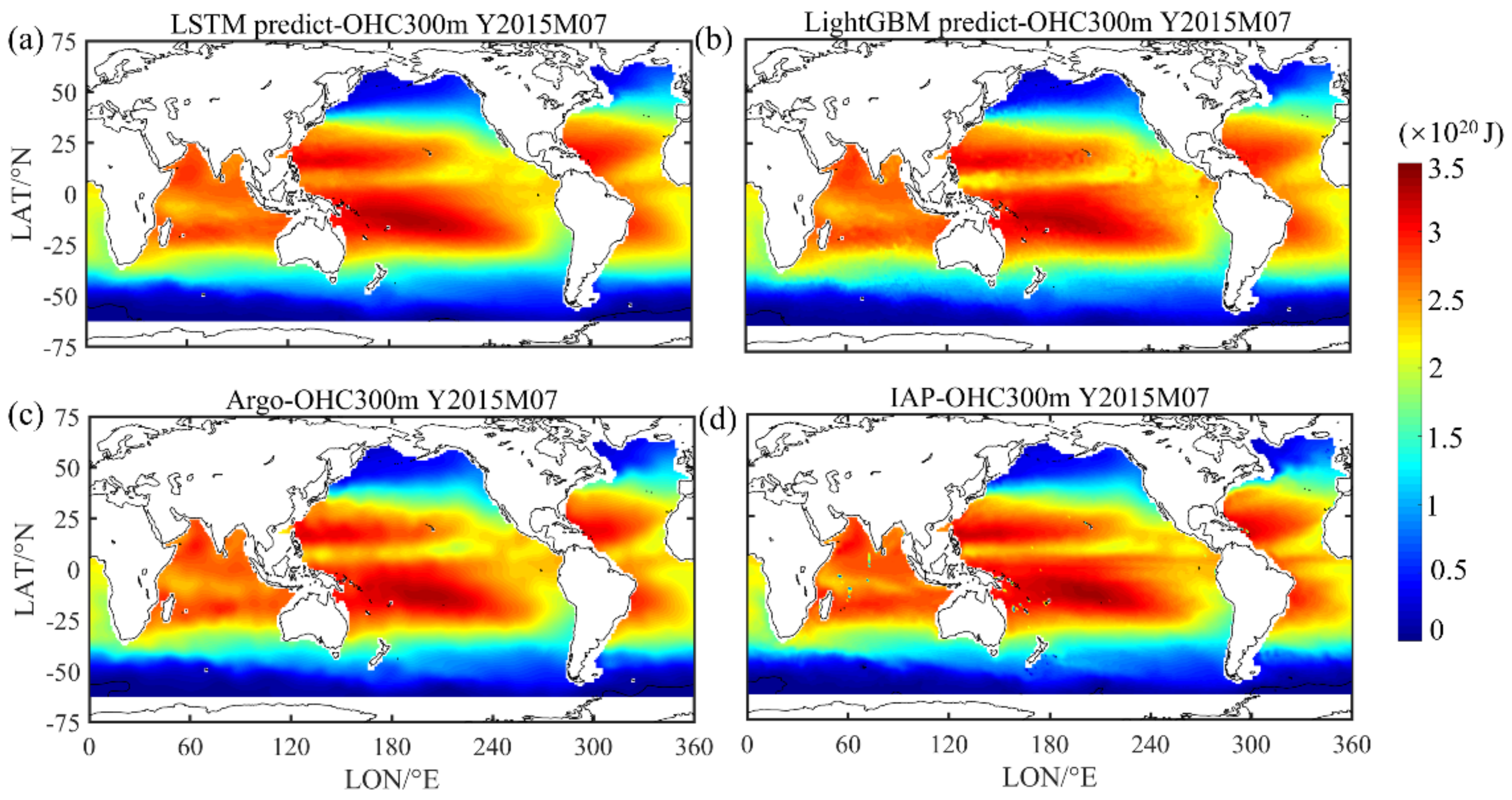
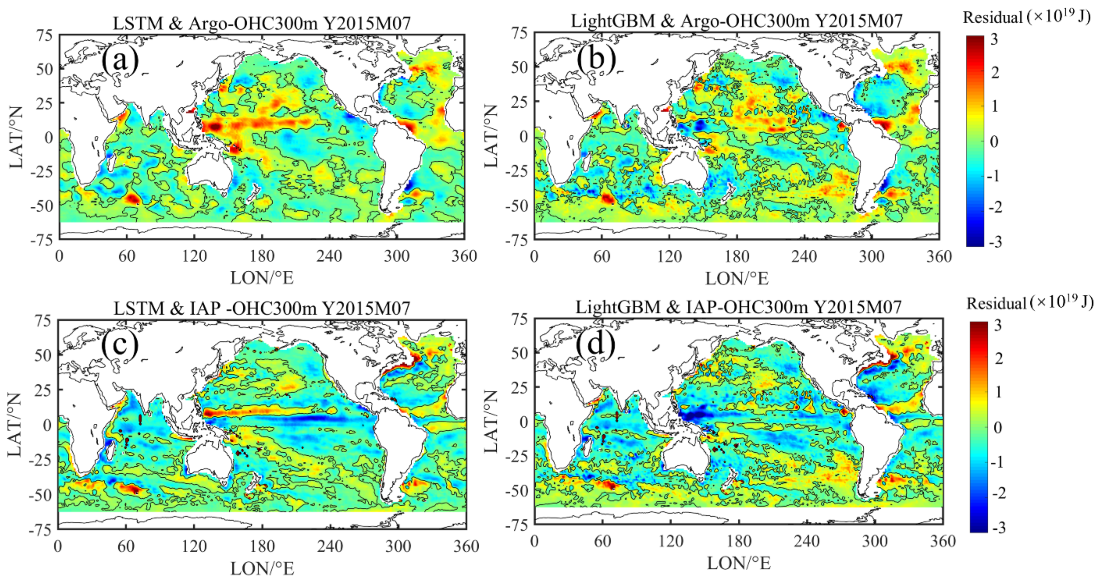
Figure 3 shows the spatial distribution of OHC300 m in the monotemporal prediction in July 2015, retrieved by the LSTM and LightGBM models, compared with Argo and IAP validation data. Overall, the accuracy of the two models relative to the Argo gridded data is as follows: RMSE = 5.85 × 10¹⁸ and R2 = 0.9964 for LSTM and RMSE = 6.31 × 10¹⁸, and R2 = 0.9959 for LightGBM. The spatial distribution of bias (“LSTM & Argo” refers to LSTM-estimated OHC minus the Argo gridded data, “LSTM & IAP” refers to LSTM-estimated OHC minus the IAP data, and so on) between our models and validation datasets is shown in Figure 4. The bias is not significant in the Indian Ocean, but it is distinctive in the equatorial Pacific Ocean, the Southern Ocean and the Northern Atlantic Ocean. This may be related to complex ocean–atmosphere interactions and the large-scale ocean circulation in these areas (i.e., El Niño and the Antarctic Circumpolar Current) [34,52]. These natural internal climate variabilities and ocean circulations influence heat redistribution. On the whole, most of the bias show green with small values close to zero. The pattern of bias from the LSTM model exhibits more even and continuous output than that of LightGBM (Figure 4).
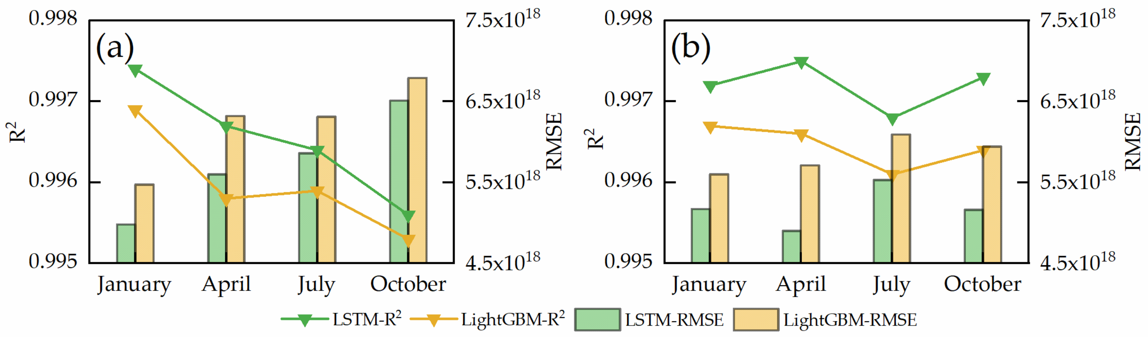
Figure 5 shows the prediction accuracy change in two years (2015 and 2018) in different seasons. The accuracy of the LSTM is higher than LightGBM for each season in 2015 and 2018 thanks to the combined use of R2 and RMSE, suggesting that LSTM outperforms LightGBM for OHC estimations. However, for different seasons, the accuracy changes of the two models are consistent; this may be related to the seasonal variability of the oceanic environment. In 2015, the prediction accuracy decreased with the seasons. In fact, El Niño experienced a rapid development in this year. In 2018, the prediction accuracy of the two models fluctuated with the seasons; RMSE in July was the highest, and in April was the lowest. In this year, the ENSO phase transformed from negative into positive, i.e., from La Niña to El Niño. Furthermore, intensive circulation processes may also affect the prediction performance of the model [46]. We found that the accuracy of the two models decreased when complex ocean–atmosphere interactions were considered, which would interfere with the model training. During the experiment, we found that the warming signal intensities detected by the two models were lower than the warming intensity of IAP, and that the model predicted OHC was underestimated compared with that of the IAP data (Figure 4c,d). However, regardless of the temporal predictions, LSTM was slightly better than LightGBM. With increasing depths, the prediction ability of LightGBM was significantly lower than that of LSTM (Table 3 and Table 4), reflecting the advantages of LSTM in deep-sea OHC retrieval.
4.2. Long-Term Reconstruction
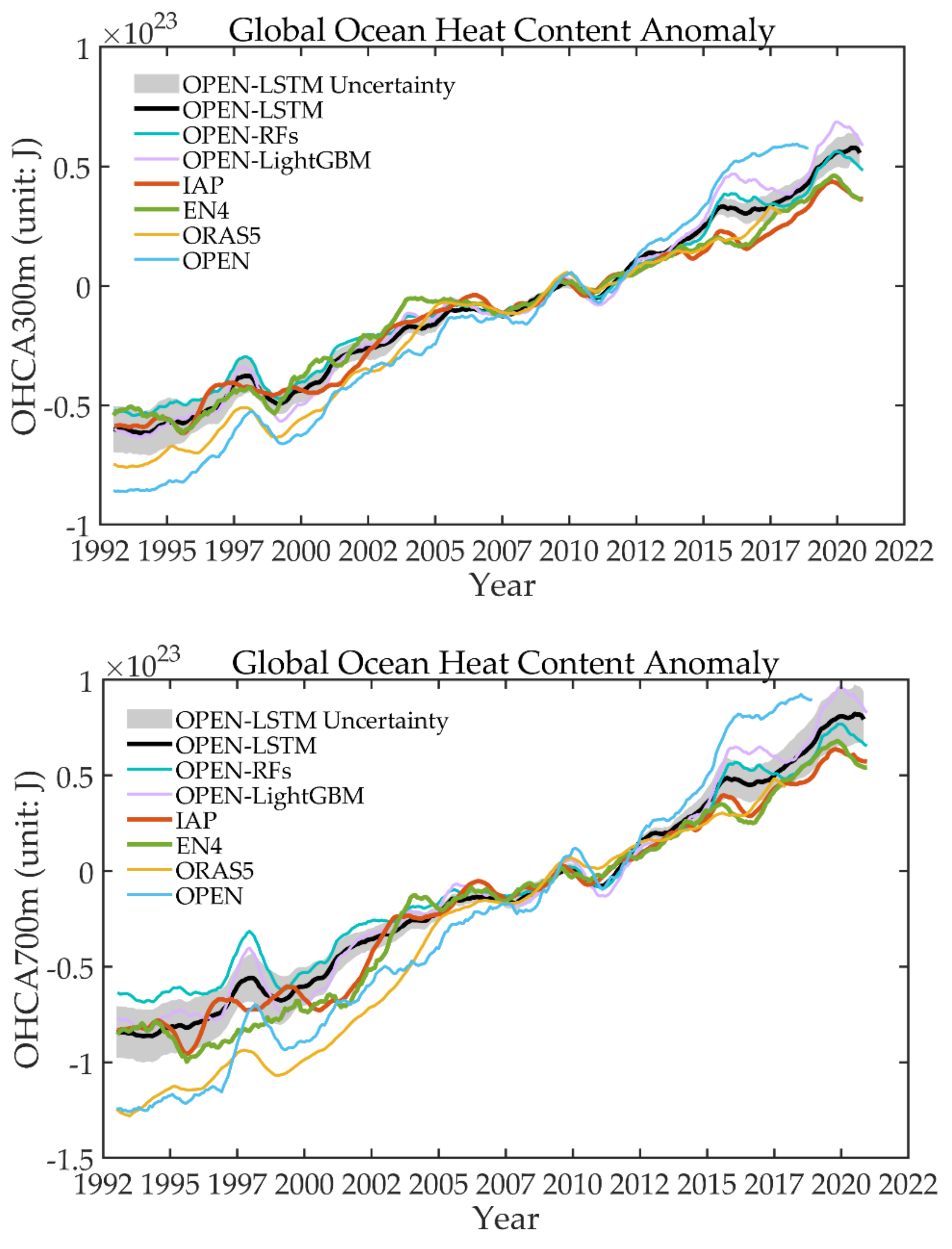
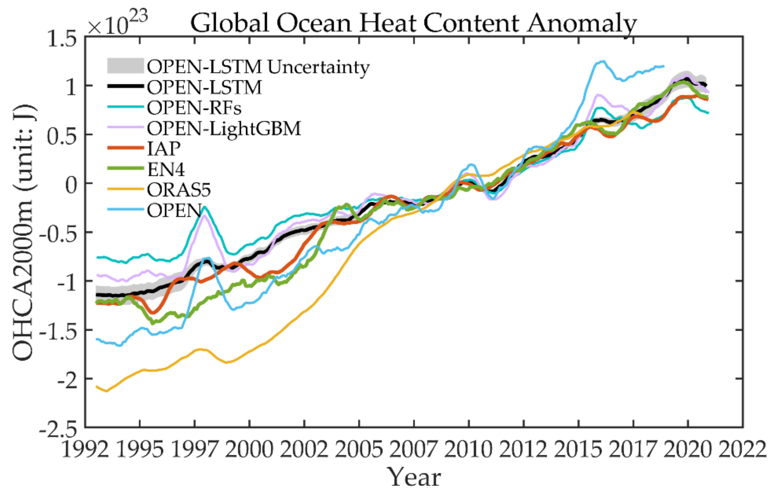
Finally, the LSTM and LightGBM model was executed to reconstruct the long time-series OHC from 1993–2020 and fill the pre-Argo data gaps. Here, a classic RFs was supplemented as a comparison to validate the reliability of the LSTM model. We adopted different algorithms and datasets for comparison and validation. Figure 6 shows the long-term OHCA prediction results (2005–2014 baseline period) in the upper 2000 m based on the LSTM, LightGBM and RFs models, which were simultaneously compared with those from existing well-known datasets (IAP, EN4, ORAS5 and OPEN). In the upper 100 m, the heat content varied greatly with the time-series and reached high values during 1997–1998 and 2015–2016 for all datasets. The heat content increased steadily from 2000 to 2010 and 2012 to 2015, showing that the ocean kept storing heat during the period. More specifically, a similar increase in 2017–2020 was revealed in all datasets, which consistently demonstrated significant and large-scale warming. In the upper 300 m, the inversion results show that all products experienced an increase at each OHC depth starting in 1993, revealing a robust warming signal in the ocean. However, the warming rate was not identical in all datasets. The black line represents the LSTM prediction result in this study (called OPEN-LSTM). The gray range is the uncertainty, i.e., twice the standard deviation of the five different ensembles of training datasets sliding back one year at a time. The purple and green lines represent the results of the machine learning method LightGBM and RFs (called OPEN-LightGBM and OPEN-RFs). The red, green, and yellow lines represent IAP, EN4, and ORAS5 data, respectively. The blue line denotes the OPEN dataset. It can be seen that the OPEN-LSTM is more consistent with the IAP and EN4 datasets than the OPEN-LightGBM and OPEN-RFs, as well as the OPEN data.
In the upper 700 m and 2000 m, the OPEN-LightGBM and OPEN-RFs datasets were significantly different in 1997–1998, and appeared higher after 2015, the same tendency as the OPEN dataset (compared with IAP and EN4 datasets). The deviation and abnormality of the reconstruction of the two models in 1997–1998 and 2015–2016 may have been caused by strong El Niño, resulting in poor model training in the sea subsurface. However, LSTM can deal with long time-series data reconstruction using its gate control structure to better predict results. The OPEN data may have been affected by the structure of the ANN model, and the parameters were not tuned appropriately for time-series prediction. The uncertainty decreases below 1000 m, which may be caused by the weakened predictive ability in the ocean’s interior and the stability of the physical, dynamic factors inside the ocean. Generally, a high level of consistency for monthly OHCA change between the OPEN-LSTM and well-known datasets (IAP, EN4) shows that LSTM is robust and performs best in long-term OHC predictions.
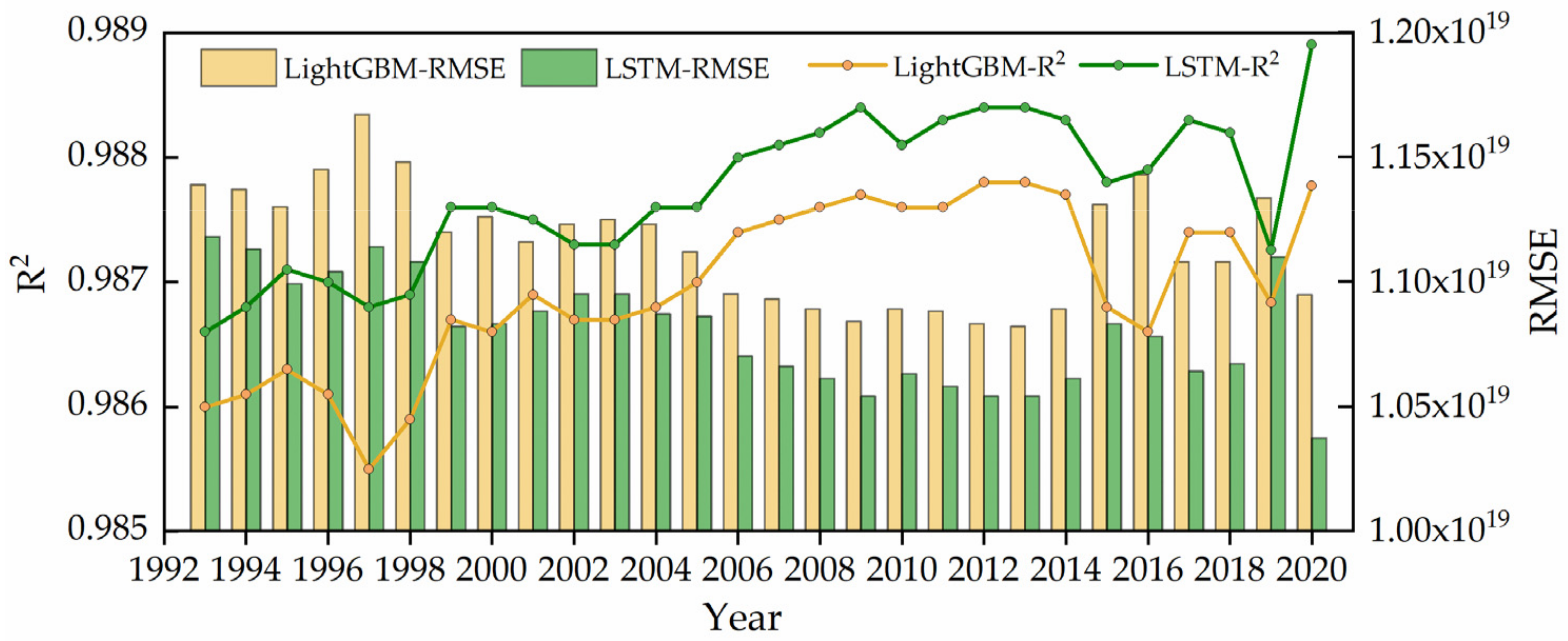
Since the time-series trends of OPEN-LightGBM and OPEN-RFs are close, and LightGBM has higher accuracy than RFs, here, we only chose OPEN-LightGBM to compare with OPEN-LSTM. We calculated the correlation of the time-series results of the two models with IAP data. Overall, LSTM was better than LightGBM for different depth ranges, and the lowest R2 and maximum RMSE at different depths were both in 1997 and 2015. In the long time-series (from 1993 to 2020), LSTM yielded superior results (the average RMSE values were 3.81 × 10¹⁸ for OHC100 m; 1.08 × 10¹⁹ for OHC300 m; 2.23 × 10¹⁹ for OHC700 m; 3.02 × 10¹⁹ for OHC1000 m; 3.72 × 10¹⁹ for OHC1500 m; and 4.45 × 10¹⁹ for OHC2000 m) than that of LightGBM (the average RMSE values were 3.90 × 10¹⁸ for OHC100 m; 1.12 × 10¹⁹ for OHC300 m; 2.31 × 10¹⁹ for OHC700 m; 3.27 × 10¹⁹ for OHC1000 m; 3.87 × 10¹⁹ for OHC1500 m; and 4.56 × 10¹⁹ for OHC2000 m) (Table 5). Figure 7 shows the accuracy of LSTM and LightGBM for OHC300 m from 1993 to 2020. In general, the results show that OPEN-LSTM has the smallest degree of error and the highest accuracy. The accuracy of the LightGBM model is inferior to that of LSTM.
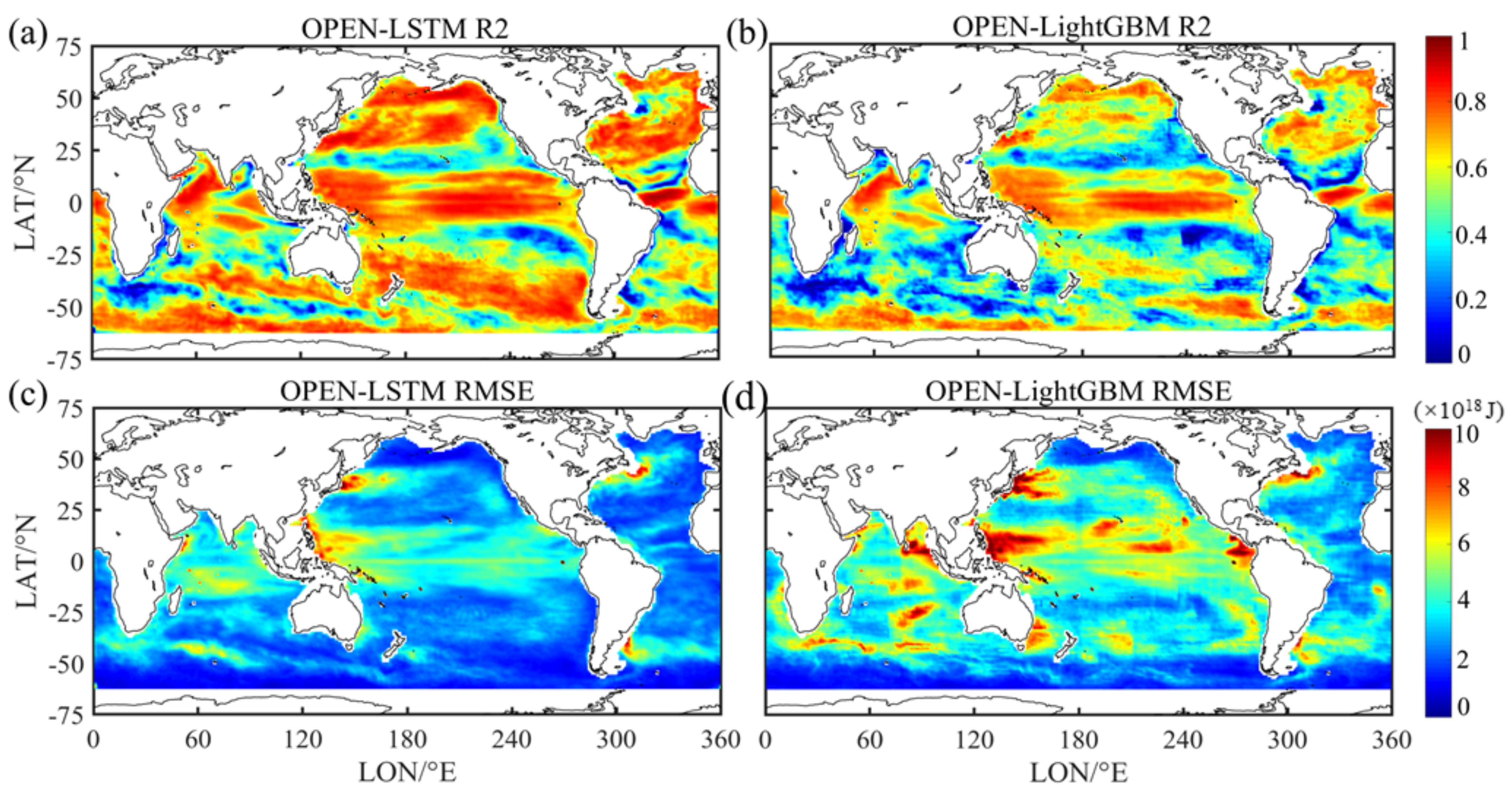
Figure 8 shows the spatial distributions of the spatiotemporal error for OHC300 m from 1993 to 2020 using OPEN-LSTM and OPEN-LightGBM with IAP data. The accuracy R2 of the two models is overall greater than 0.4. However, the spatial distributions of R2 (greater than 0.6) between the two estimation datasets show differences. The high correlation R2 for LSTM (greater than 0.6) implies a wider distribution than that of LightGBM in the equatorial Pacific, the north of the Pacific, the north of the Atlantic, the north of the Indian Ocean, and the Southern Ocean. The RMSE also shows that LSTM reduced the error significantly in data from the Southern and Pacific Oceans compared with LightGBM. These results may be due to the vast areas and abundant eddies in the Pacific and Southern Oceans, especially given the sparse floats observations from the Southern Ocean. In addition, the regions of the western boundary currents where many eddies occur, such as the Kuroshio (near 145° E, 42° N), the Gulf Stream (near 48° W, 45° N), and the Brazil–Malvinas Confluence Region (near 55° W, 46° S), including the region with the Antarctic Circumpolar Current, have high RMSE. Further, the Argo network distribution is insufficient in high-latitude oceans and marginal seas, showing some differences in these areas in these two datasets. The spatiotemporal error indicates that LSTM has advantages in time-series and global-scale reconstruction.
4.3. The Relative Error in Different Basin Scales
The choice of baseline climatology is essential in studying historical OHC change. The climatological standard selected in this paper was 2005–2014, but this happens to also be the model training period (Figure 6). The period for ORAS5 is from 1979 to 2018. So, we calculated the relative error (the average value for the Argo data subtracted from the average value of the estimated or validated datasets and divided by the former value) from 2005 to 2018. Figure 9 and Figure 10 show the relative error of the models-estimated datasets at different depths and ocean basins and compared with those of other datasets (IAP, EN4 and ORAS5).
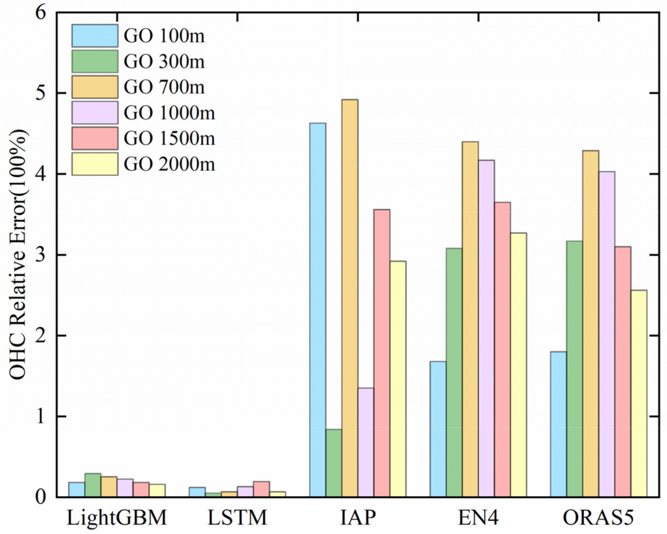
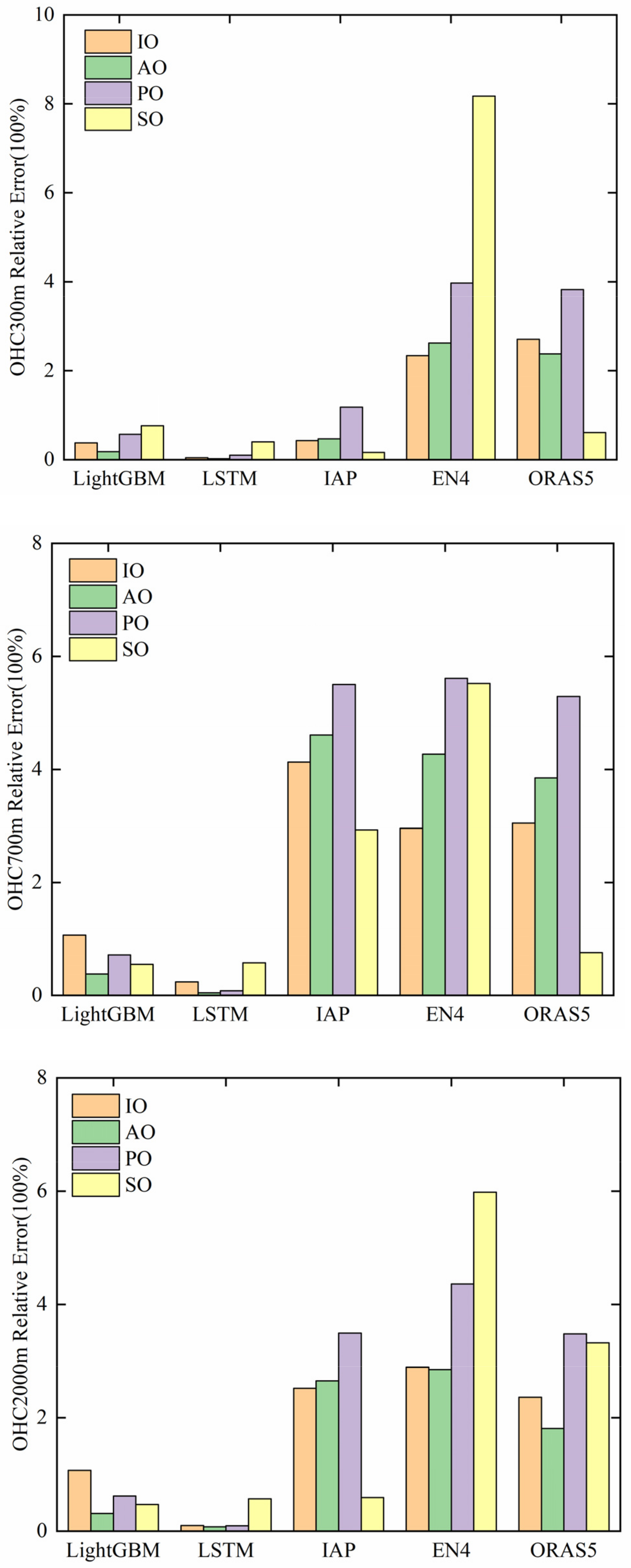
For different depths in the global ocean, the value of the relative error for LSTM was the smallest in these datasets (Figure 9). The value between EN4 and ORAS5 was similar for different depths, and the error was larger in 0–700 and 0–1000 m. The value for IAP changed significantly, and the error was larger at 0–100 m and 0–700 m. For different ocean basins, the value of the estimated dataset OPEN-LSTM was slightly lower than that of OPEN-LightGBM at different depth ranges and basins (Figure 10). For OHC100 m and 300 m, the value for EN4 in the Southern Ocean was higher than those of other basins and datasets; this may have been due to the XBT instrument bias, and the fact that the instrument detect depth was above 700 m. As the depth increased, the value for validation datasets was large in the Pacific Ocean and the Southern Ocean. For OPEN-LSTM, the error was mainly in the Southern Ocean. But for OPEN-LightGBM, the error was mainly distributed in the Indian Ocean, the Pacific Ocean, and the Southern Ocean below 700 m. In summary, the relative error of LSTM was less than that of LightGBM and those of IAP, EN4, and ORAS5 over the four ocean basins, while the accuracy of OPEN-LSTM was the closest to that of the Argo gridded data.
4.4. OHC Changes in Different Periods and Depths
This study calculated the average global warming trend for OHC in different periods (pre-Argo period, 1993–2004; long time-series, 1993–2020) and depths for several datasets to quantitatively evaluate the global warming variability of OHC (Table 6). As the depth increased, the difference for the model-estimated datasets and validation datasets became more significant. However, the OPEN-LSTM dataset was more consistent with IAP, EN4 and ORAS5 than OPEN-LightGBM and OPEN-RFs at different periods and depth ranges. Moreover, the OPEN-RFs dataset contained significant underestimations compared to the other datasets. It is worth noting that the average global warming trend for OHC in 1993–2020 was very close in the OPEN-LSTM and IAP datasets.
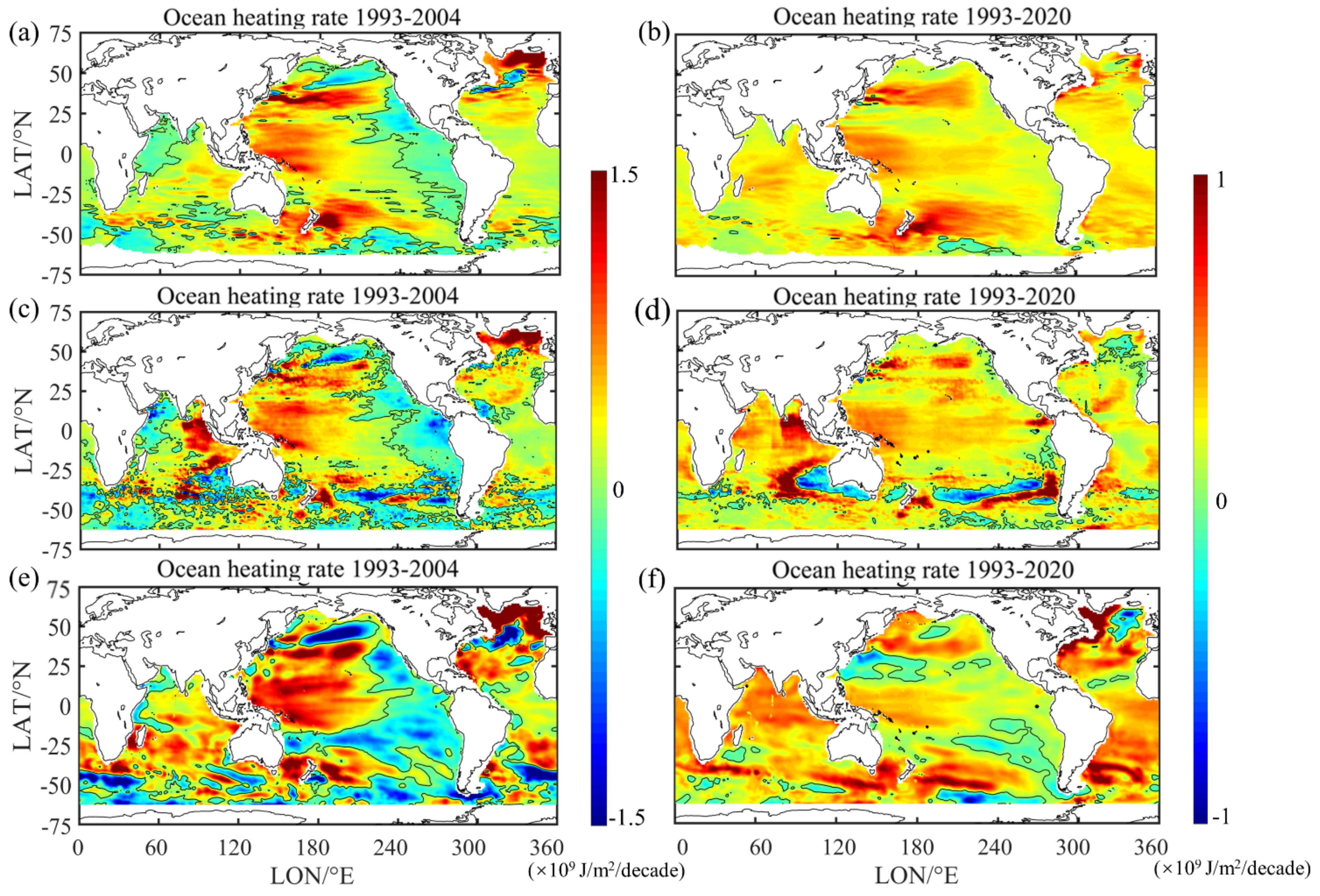
Figure 11 shows the linear trends of OHC changes from three datasets (OPEN-LSTM, OPEN-LightGBM and IAP) during the 1993 to 2004 and 1993 to 2020 periods. From 1993 to 2004, the signals from three datasets were generally consistent. Warming signals were evident in the western Pacific Ocean, Southern Ocean, North Atlantic Ocean and eastern Indian Ocean. Cooling signals were observed in the eastern Pacific Ocean, Southern Ocean, and Western Indian Ocean. From 1993 to 2020, the significant difference was that the IAP dataset exhibited more distinctive warmer signals in the Atlantic, Indian and Southern Oceans compared to the other datasets. In addition, the OPEN-LightGBM dataset showed two cooling signals in the Southern Ocean, while the IAP and OPEN-LSTM did not. However, the signal intensities for the OPEN-LSTM dataset were weaker in some regions than those of IAP in both the pre-Argo and long time-series.
Additionally, for the EN4 and ORAS5 datasets, the trends of OHC changes from 1993 to 2020 were slightly higher than those of OPEN-LSTM, and presented more significant spatial heterogeneity on a global scale. The ocean warming rate during different periods for different datasets exhibited some differences, but the OPEN-LSTM dataset was most consistent with IAP in terms of the general trend of OHC change.
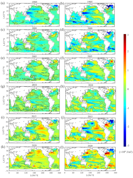
Figure 12 shows the OHC anomaly for different years (1995, 2000, 2005, 2010, 2015, and 2020) from two datasets (OPEN-LSTM and IAP) in the upper 2000 m. The OPEN-LSTM was much weaker than the IAP product in the time-series. Generally, the two datasets showed consistent OHC anomaly patterns in each year. From 1995 to 2020, the ocean warmed in the eastern Pacific, Southern, western Atlantic and North Indian Oceans. The anomaly patterns in OPEN-LSTM were less significant than those in the EN4 and ORAS5 datasets on a global scale, but more similar to those in the IAP dataset. The OHC anomaly patterns for the validation datasets presented more significant spatial heterogeneity (with distinct warming or cooling signals) than OPEN-LSTM on a global scale, while the OPEN-LSTM dataset, based on remote sensing, exhibited more distinctive spatial consistency in the OHC patterns than the validation datasets.
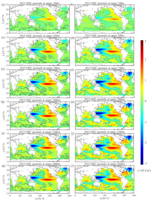
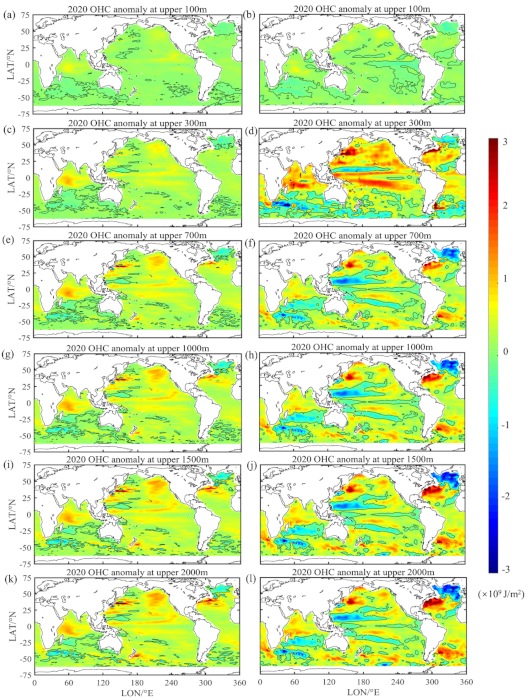
Figure 13 and Figure 14 show the OHC anomaly for different depths (100, 300, 700, 1000, 1500, and 2000 m) from two datasets (OPEN-LSTM and IAP) in 2015 and 2020. For 2015, it appeared that there were consistent patterns between the two datasets at each layer. The OHC anomaly showed an eastern cold tongue and western warm pool patterns with strong variability. As the depth increased, the anomaly signals in Gulf Stream and subpolar gyre became more significant in the IAP dataset than in the OPEN-LSTM. From the upper 700 m to upper 2000 m, the IAP dataset showed that the Southern Ocean had experienced a gradually warming, while the same signal in the OPEN-LSTM dataset was somewhat weaker. These differences may be attributed to the different production methods of the two datasets. The IAP dataset was reconstructed by temperature products based on the En-OI interpolation mapping method, while the OPEN-LSTM OHC dataset is directly predicted by a deep learning model based on satellite remote sensing combined with Argo gridded data. For 2020, the spatial distribution of the OHC anomaly for the OPEN-LSTM and IAP datasets exhibited a certain degree of inconsistency. The IAP dataset presented more significant spatial heterogeneity for the OHC pattern, but our OPEN-LSTM dataset showed a more consistent spatial pattern over a global scale, and demonstrated a stronger warming signal in the deeper layers (from 700 m to 2000 m); this is consistent with the previous studies indicating that warming in the subsurface and deeper ocean is more significant than in the upper ocean [9,10,13].
5. Conclusions
This study aimed to establish a robust and efficient model to improve the inversion accuracy of OHC based on the OPEN dataset. In this study, we proposed a deep learning method that considers temporal dependence, known as LSTM, to estimate OHC by combining remote sensing and Argo gridded data with spatial and temporal information. The parameters of the LSTM model needed to be tuned, especially the time step, which could influence the accuracy of the predictions. Additionally, the optimal time step of the model in different depth ranges was not the same. The main conclusions of this paper are as follows: (1) this study demonstrated that the performance of the LSTM model is superior compared to the LightGBM and RFs algorithms. The reconstructed OPEN-LSTM dataset showed a high level of consistency for monthly OHCA time-series change compared with the IAP and EN4 datasets; (2) the spatiotemporal error distribution of the OPEN-LSTM dataset was also lower than those of OPEN-LightGBM and OPEN-RFs on a global scale. The relative error showed that the OPEN-LSTM was more reliable than OPEN-LightGBM and OPEN-RFs compared with Argo data in different depths and basins; (3) the average global warming trend for OHC from 1993 to 2020 was similar to those in the OPEN-LSTM and IAP datasets, although there were some inconsistent patterns between the two datasets for the trends of OHC change during the 1993–2004 and 1993–2020 periods. The warming and cooling signals for OPEN-LSTM dataset were a little weaker than those of IAP, EN4 and ORAS5; (4) the OHC anomaly for the OPEN-LSTM dataset in different years and depth ranges was generally consistent with IAP. In 2020, the IAP dataset presented significant spatial heterogeneity for OHC pattern, while OPEN-LSTM showed a more consistent spatial pattern over a global scale, and exhibited a stronger warming signal in the deeper layers.
This study reconstructed the OPEN-LSTM dataset based on remote sensing and Argo data, in order to fill in gaps from the pre-Argo period and provide a new perspective for the study of global ocean warming in the upper 2000 m. For deep learning techniques, adjusting the model parameters is crucial for accurate model predictions. With the development of artificial intelligence technology, automatic parameter optimization will become essential in future studies. Additionally, considering relevant oceanic physical factors in order to more accurately determine OHC is likely to prove useful. Using model and reanalysis data will extend the time-series range, thereby facilitating the study of decadal and multidecadal periods, and will provide a deeper understanding of ocean and climate variabilities. At present, the Argo float observations only cover the global ocean for the upper 2000 m, so the prediction depth for OHC was limited in this study. In future, with the implementation of the deep-Argo plan, OHC predictions at greater depths, which are more meaningful for global climate change studies, will be possible by combining satellite remote sensing data with Argo observations.
Author Contributions
Conceptualization, H.S.; methodology, T.Q.; validation, T.Q. and A.W.; formal analysis, H.S. and T.Q.; investigation, A.W.; data curation, T.Q.; writing—original draft preparation, H.S. and T.Q.; writing—review and editing, H.S. and W.L.; visualization, T.Q.; supervision, H.S. and W.L.; funding acquisition, H.S. All authors have read and agreed to the published version of the manuscript.
Funding
This research was funded by National Natural Science Foundation of China (grant number: 41971384, 41630963), the Strategic Priority Research Program of the Chinese Academy of Sciences, CASEarth (XDA19080103).
Institutional Review Board Statement
Not applicable.
Informed Consent Statement
Not applicable.
Data Availability Statement
The data presented in this study are available on request from the corresponding author.
Acknowledgments
The authors would like to thank three anonymous reviewers for their constructive comments, which significantly improved the quality of our paper. The OPEN-LSTM dataset will be shared to the research community at Science Data Bank (ScienceDB) and can be freely accessed (http://0-www-doi-org.brum.beds.ac.uk/10.11922/sciencedb.01154, accessed on 4 July 2021).
Conflicts of Interest
The authors declare no conflict of interest.
References
- Hansen, J.; Nazarenko, L.; Ruedy, R.; Sato, M.; Willis, J.; Genio, A.; Koch, D.; Lacis, A.; Lo, K.; Menon, S.; et al. Earth’s energy imbalance: Confirmation and implications. Science 2005, 308, 1431–1435. [Google Scholar] [CrossRef] [Green Version]
- Trenberth, K.E.; Fasullo, J.T.; Kiehl, J. Earth’s Global Energy Budget. Bull. Am. Meteorol. Soc. 2009, 90, 311–324. [Google Scholar] [CrossRef]
- Gastineau, G.; Friedman, A.R.; Khodri, M.; Vialard, J. Global ocean heat content redistribution during the 1998-2012 Interdecadal Pacific Oscillation negative phase. Clim. Dyn. 2019, 53, 1187–1208. [Google Scholar] [CrossRef] [Green Version]
- Kaufman, D.; McKay, N.; Routson, C.; Erb, M.; Dätwyler, C.; Sommer, P.S.; Heiri, O.; Davis, B. Holocene global mean surface temperature, a multi-method reconstruction approach. Sci. Data 2020, 7, 201. [Google Scholar] [CrossRef]
- Cheng, L.; Zhu, J. 2017 was the Warmest Year on Record for the Global Ocean. Adv. Atmos. Sci. 2018, 34, 261–263. [Google Scholar] [CrossRef] [Green Version]
- Cheng, L.; Zhu, J.; Abraham, J.; Trenberth, K.E.; Fasullo, J.T.; Zhang, B.; Yu, F.; Wan, L.; Chen, X.; Song, X. 2018 Continues Record Global Ocean Warming. Adv. Atmos. Sci. 2019, 36, 249–252. [Google Scholar] [CrossRef] [Green Version]
- Cheng, L.; Abraham, J.; Zhu, J.; Trenberth, K.E.; Fasullo, J.; Boyer, T.; Locarnini, R.; Zhang, B.; Yu, F.; Wan, L.; et al. Record-Setting Ocean Warmth Continued in 2019. Adv. Atmos. Sci. 2020, 37, 137–142. [Google Scholar] [CrossRef] [Green Version]
- Cheng, L.; Abraham, J.; Trenberth, K.E.; Fasullo, J.; Boyer, T.; Locarnini, R.; Zhang, B.; Yu, F.; Wan, L.; Chen, X.; et al. Upper Ocean Temperatures Hit Record High in 2020. Adv. Atmos. Sci. 2021, 38, 523–530. [Google Scholar] [CrossRef]
- Yan, X.-H.; Boyer, T.; Trenberth, K.; Karl, T.R.; Xie, S.-P.; Nieves, V.; Tung, K.-K.; Roemmich, D. The global warming hiatus: Slowdown or redistribution? Earth’s Future 2016, 4, 472–482. [Google Scholar] [CrossRef] [PubMed]
- Cheng, L.; Abraham, J.; Hausfather, Z.; Trenberth, K.E. How fast are the oceans warming? Sci. (Am. Assoc. Adv. Sci.) 2019, 363, 128–129. [Google Scholar] [CrossRef] [PubMed]
- Liu, W.; Xie, S.-P.; Lu, J. Tracking ocean heat uptake during the surface warming hiatus. Nat. Commun. 2016, 7, 10926. [Google Scholar] [CrossRef] [Green Version]
- Trenberth, K.E.; Fasullo, J.T. An apparent hiatus in global warming? Earth’s Future 2013, 1, 19–32. [Google Scholar] [CrossRef]
- Su, H.; Wu, X.; Lu, W.; Zhang, W.; Yan, X.-H. Inconsistent Subsurface and Deeper Ocean Warming Signals During Recent Global Warming and Hiatus. J. Geophys. Res. Ocean. 2017, 122, 8182–8195. [Google Scholar] [CrossRef]
- Stocker, T.F.; Qin, D.; Plattner, G.-K.; Tignor, M.M.B.; Allen, S.K.; Boschung, J.; Nauels, A.; Xia, Y.; Bex, V.; Midgley, P.M. (Eds.) Climate Change 2013: The Physical Science Basis; IPCC; Cambridge University Press: Cambridge, UK; New York, NY, USA, 2013. [Google Scholar]
- Meehl, G.A.; Arblaster, J.M.; Fasullo, J.T.; Hu, A.; Trenberth, K.E. Model-based evidence of deep-ocean heat uptake during surface-temperature hiatus periods. Nat. Clim. Chang. 2011, 1, 360–364. [Google Scholar] [CrossRef]
- Cheng, L.; Trenberth, K.E.; Fasullo, J.; Boyer, T.; Abraham, J.; Zhu, J. Improved estimates of ocean heat content from 1960 to 2015. Sci. Adv. 2017, 3, e1601545. [Google Scholar] [CrossRef] [PubMed] [Green Version]
- Shukla, P.R.; Skea, J.; Calvo Buendia, E.; Masson-Delmotte, V.; Pörtner, H.-O.; Roberts, D.C.; Zhai, P.; Slade, R.; Connors, S.; Van Diemen, R.; et al. (Eds.) IPCC (2019): Summary for Policymakers: Special Report on the Ocean and Cryosphere in a Changing Climate; 2019; in press. [Google Scholar]
- Von Schuckmann, K.; Palmer, M.D.; Trenberth, K.E.; Cazenave, A.; Chambers, D.; Champollion, N.; Hansen, J.; Josey, S.A.; Loeb, N.; Mathieu, P.-P.; et al. An imperative to monitor Earth’s energy imbalance. Nat. Clim. Chang. 2016, 6, 138–144. [Google Scholar] [CrossRef] [Green Version]
- Meyssignac, B.; Boyer, T.; Zhao, Z.; Hakuba, M.Z.; Landerer, F.W.; Stammer, D.; Köhl, A.; Kato, S.; L’Ecuyer, T.; Ablain, M.; et al. Measuring Global Ocean Heat Content to Estimate the Earth Energy Imbalance. Front. Mar. Sci. 2019, 6, 432. [Google Scholar] [CrossRef] [Green Version]
- Rydbeck, A.V.; Jensen, T.G.; Smith, T.A.; Flatau, M.K.; Janiga, M.A.; Reynolds, C.A.; Ridout, J.A. Ocean Heat Content and the Intraseasonal Oscillation. Geophys. Res. Lett. 2019, 46, 14558–14566. [Google Scholar] [CrossRef]
- Zhang, L.; Han, W.; Li, Y.; Lovenduski, N.S. Variability of Sea Level and Upper-Ocean Heat Content in the Indian Ocean: Effects of Subtropical Indian Ocean Dipole and ENSO. J. Clim. 2019, 32, 7227–7245. [Google Scholar] [CrossRef]
- Hallam, S.; Guishard, M.; Josey, S.A.; Hyder, P.; Hirschi, J. Increasing tropical cyclone intensity and potential intensity in the subtropical Atlantic around Bermuda from an ocean heat content perspective 1955–2019. Environ. Res. Lett. 2021, 16, 034052. [Google Scholar] [CrossRef]
- Gronholz, A.; Dong, S.; Lopez, H.; Lee, S.K.; Goni, G.; Baringer, M. Interannual Variability of the South Atlantic Ocean Heat Content in a High-Resolution Versus a Low-Resolution General Circulation Model. Geophys. Res. Lett. 2020, 47, e2020GL089908. [Google Scholar] [CrossRef]
- Abraham, J.P.; Baringer, M.; Bindoff, N.L.; Boyer, T.; Cheng, L.J.; Church, J.A.; Conroy, J.L.; Domingues, C.M.; Fasullo, J.T.; Gilson, J.; et al. A review of global ocean temperature observations: Implications for ocean heat content estimates and climate change. Rev. Geophys. 2013, 51, 450–483. [Google Scholar] [CrossRef]
- Lyman, J.M.; Willis, J.K.; Johnson, G.C. Recent cooling of the upper ocean. Geophys. Res. Lett. 2006, 33, L18604. [Google Scholar] [CrossRef] [Green Version]
- Boyer, T.; Domingues, C.M.; Good, S.A.; Johnson, G.C.; Lyman, J.M.; Ishii, M.; Gouretski, V.; Willis, J.K.; Antonov, J.; Wijffels, S.; et al. Sensitivity of Global Upper-Ocean Heat Content Estimates to Mapping Methods, XBT Bias Corrections, and Baseline Climatologies. J. Clim. 2016, 29, 4817–4842. [Google Scholar] [CrossRef]
- Klemas, V.; Yan, X.-H. Subsurface and deeper ocean remote sensing from satellites: An overview and new results. Prog. Oceanogr. 2013, 11, 010. [Google Scholar] [CrossRef]
- Wang, J.; Flierl, G.R.; LaCasce, J.H.; McClean, J.L.; Mahadevan, A. Reconstructing the Ocean’s Interior from Surface Data. J. Phys. Oceanogr. 2013, 43, 1611–1626. [Google Scholar] [CrossRef]
- Meinen, C.S. Structure of the North Atlantic current in stream-coordinates and the circulation in the Newfoundland basin. Deep-Sea Res. Part I Oceanogr. Res. Pap. 2001, 48, 1553–1580. [Google Scholar] [CrossRef]
- Balmaseda, M.A.; Trenberth, K.E.; Källén, E. Distinctive climate signals in reanalysis of global ocean heat content. Geophys. Res. Lett. 2013, 40, 1754–1759. [Google Scholar] [CrossRef]
- Carton, J.A.; Giese, B.S. A Reanalysis of Ocean Climate Using Simple Ocean Data Assimilation (SODA). Mon. Weather Rev. 2008, 136, 2999–3017. [Google Scholar] [CrossRef]
- Su, H.; Wu, X.; Yan, X.-H.; Kidwell, A. Estimation of subsurface temperature anomaly in the Indian Ocean during recent global surface warming hiatus from satellite measurements: A support vector machine approach. Remote Sens. Environ. 2015, 160, 63–71. [Google Scholar] [CrossRef]
- Su, H.; Li, W.; Yan, X.-H. Retrieving Temperature Anomaly in the Global Subsurface and Deeper Ocean From Satellite Observations. J. Geophys. Res. Ocean. 2017, 123, 399–410. [Google Scholar] [CrossRef]
- Su, H.; Yang, X.; Lu, W.; Yan, X.-H. Estimating Subsurface Thermohaline Structure of the Global Ocean Using Surface Remote Sensing Observations. Remote Sens. 2019, 11, 1598. [Google Scholar] [CrossRef] [Green Version]
- Su, H.; Huang, L.; Li, W.; Yang, X.; Yan, X.-H. Retrieving Ocean Subsurface Temperature Using a Satellite-Based Geographically Weighted Regression Model. J. Geophys. Res. Ocean. 2018, 123, 5180–5193. [Google Scholar] [CrossRef]
- Lu, W.; Su, H.; Yang, X.; Yan, X.-H. Subsurface temperature estimation from remote sensing data using a clustering-neural network method. Remote Sens. Environ. 2019, 229, 213–222. [Google Scholar] [CrossRef]
- Chacko, N.; Dutta, D.; Ali, M.M.; Sharma, J.R.; Dadhwal, V.K. Near-Real-Time Availability of Ocean Heat Content Over the North Indian Ocean. IEEE Geosci. Remote Sens. Lett. 2015, 12, 1033–1036. [Google Scholar] [CrossRef]
- Jagadeesh, P.S.V.; Suresh Kumar, M.; Ali, M.M. Estimation of Heat Content and Mean Temperature of Different Ocean Layers. IEEE J. Sel. Top. Appl. Earth Obs. Remote Sens. 2015, 8, 1251–1255. [Google Scholar] [CrossRef]
- Irrgang, C.; Saynisch, J.; Thomas, M. Estimating global ocean heat content from tidal magnetic satellite observations. Sci. Rep. 2019, 9, 7893. [Google Scholar] [CrossRef] [PubMed] [Green Version]
- Su, H.; Zhang, H.; Geng, X.; Qin, T.; Lu, W.; Yan, X. OPEN: A New Estimation of Global Ocean Heat Content for Upper 2000 Meters from Remote Sensing Data. Remote Sens. 2020, 12, 2294. [Google Scholar] [CrossRef]
- Yang, Y.; Dong, J.; Sun, X.; Lima, E.; Mu, Q.; Wang, X. A CFCC-LSTM Model for Sea Surface Temperature Prediction. IEEE Geosci. Remote Sens. Lett. 2018, 15, 207–211. [Google Scholar] [CrossRef]
- Song, T.; Jiang, J.; Li, W.; Xu, D. A Deep Learning Method With Merged LSTM Neural Networks for SSHA Prediction. IEEE J. Sel. Top. Appl. Earth Obs. Remote Sens. 2020, 13, 2853–2860. [Google Scholar] [CrossRef]
- Zhang, Q.; Wang, H.; Dong, J.; Zhong, G.; Sun, X. Prediction of Sea Surface Temperature Using Long Short-Term Memory. IEEE Geosci. Remote Sens. Lett. 2017, 14, 1745–1759. [Google Scholar] [CrossRef] [Green Version]
- Sarkar, P.P.; Janardhan, P.; Roy, P. Prediction of sea surface temperatures using deep learning neural networks. SN Appl. Sci. 2020, 2, 1458. [Google Scholar] [CrossRef]
- Good, S.A.; Martin, M.J.; Rayner, N.A. EN4: Quality controlled ocean temperature and salinity profiles and monthly objective analyses with uncertainty estimates. J. Geophys. Res. Ocean. 2013, 118, 6704–6716. [Google Scholar] [CrossRef]
- Jeong, Y.; Hwang, J.; Park, J.; Jang, C.J.; Jo, Y. Reconstructed 3-D Ocean Temperature Derived from Remotely Sensed Sea Surface Measurements for Mixed Layer Depth Analysis. Remote Sens. 2019, 11, 3018. [Google Scholar] [CrossRef] [Green Version]
- Hochreiter, S.; Schmidhuber, J. Long short-term memory. Neural Comput. 1997, 9, 1735–1780. [Google Scholar] [CrossRef] [PubMed]
- Gers, F.A.; Schmidhuber, J.; Cummins, F. Learning to forget: Continual prediction with LSTM. Neural Comput. 2000, 12, 2451–2471. [Google Scholar] [CrossRef] [PubMed]
- Huang, A.; Vega-Westhoff, B.; Sriver, R.L. Analyzing El Niño-Southern Oscillation Predictability Using Long-Short-Term-Memory Models. Earth Space Sci. 2019, 6, 212–221. [Google Scholar] [CrossRef]
- Ke, G.L.; Meng, Q.; Finley, T.; Wang, T.F.; Chen, W.; Ma, W.D.; Ye, Q.W.; Liu, T.Y. LightGBM: A Highly Efficient Gradient Boosting Decision Tree. In Proceedings of the 31st International Conference on Neural Information Processing Systems, Long Beach, CA, USA, 4–9 December 2017; pp. 3149–3157. [Google Scholar]
- Breiman, L. Random forests. Mach. Learn. 2001, 45, 5–32. [Google Scholar] [CrossRef] [Green Version]
- Wang, G.; Cheng, L.; Abraham, J.; Li, C. Consensuses and discrepancies of basin-scale ocean heat content changes in different ocean analyses. Clim. Dyn. 2018, 50, 2471–2487. [Google Scholar] [CrossRef] [Green Version]
Figure 1.
LSTM performance according to the number of layers and hidden units measured with loss function MAE in OHC300 m retrieval. The different colored lines denote the MAE with different hidden units (20, 60, 100, 120, 140, 160) in the LSTM layer. (a) Denotes the MAE with only one layer, (b) denotes the MAE with two layers based on the previous layer as the epoch increases. Line 20 means that there are 20 hidden units in the current layer; line 60 means there are 60 hidden units in the current layer, and so on. The lines in the figure have been smoothed by a running mean filter.

Figure 2.
LSTM performance for the time step measured with the RMSE in OHC300 m retrieval. The histogram represents the RMSE with different time steps (1–12 months) in the LSTM model. Unit: J.
Figure 2.
LSTM performance for the time step measured with the RMSE in OHC300 m retrieval. The histogram represents the RMSE with different time steps (1–12 months) in the LSTM model. Unit: J.

Figure 3.
OHC spatial distribution in the upper 300 m in July 2015 from the (a) LSTM and (b) LightGBM model predictions and the (c) Argo and (d) IAP validation datasets. Unit: J.
Figure 3.
OHC spatial distribution in the upper 300 m in July 2015 from the (a) LSTM and (b) LightGBM model predictions and the (c) Argo and (d) IAP validation datasets. Unit: J.

Figure 4.
Spatial distribution of bias between our model-estimated results and validation dataset for OHC300 m in July 2015. (a) is the bias between LSTM and Argo gridded data, (b) is the bias between LightGBM and Argo gridded data, (c) is the bias between LSTM and IAP data, and (d) is the bias between LightGBM and IAP data. Unit: J.

Figure 5.
Accuracy of OHC300 m in (a) 2015 and (b) 2018 in different seasons from the LSTM and LightGBM models compared with the Argo data. Lines and histograms with different colors are the R2 and RMSE from different models. RMSE Unit: J.
Figure 5.
Accuracy of OHC300 m in (a) 2015 and (b) 2018 in different seasons from the LSTM and LightGBM models compared with the Argo data. Lines and histograms with different colors are the R2 and RMSE from different models. RMSE Unit: J.

Figure 6.
Monthly OHCA time-series in the upper 300 m, 700 m, 2000 m in the global ocean from different model-estimated results and validation datasets from 1993 to 2020. Different lines represent different datasets. The black line represents the LSTM model-estimated results (named OPEN-LSTM). The green line represents the RFs model-estimated results (named OPEN-RFs). The purple line represents the LightGBM model-estimated results (named OPEN-LightGBM). The red, green, yellow lines represent three validation datasets, IAP, EN4, ORAS5. The blue line represents the compared ANN-based OPEN dataset. Gray shading is the uncertainty for twice the standard deviation (±2σ) of the training dataset sliding back five ensembles per one-year stride. Twelve-month running means were used to filter high-frequency signals. The baseline of the time series is 2005–2014. Unit: J.


Figure 7.
Accuracy R2 and RMSE of the OPEN-LSTM and OPEN-LightGBM results for the long time-series OHC300 m from 1993 to 2020 compared with those of IAP. RMSE Unit: J.
Figure 7.
Accuracy R2 and RMSE of the OPEN-LSTM and OPEN-LightGBM results for the long time-series OHC300 m from 1993 to 2020 compared with those of IAP. RMSE Unit: J.

Figure 8.
Spatial error distributions of the OPEN-LSTM and OPEN-LightGBM datasets in each 1° × 1° grid of OHC300 m from 1993 to 2020 compared with those of IAP. RMSE Unit: J.
Figure 8.
Spatial error distributions of the OPEN-LSTM and OPEN-LightGBM datasets in each 1° × 1° grid of OHC300 m from 1993 to 2020 compared with those of IAP. RMSE Unit: J.

Figure 9.
The relative error of several datasets compared with Argo gridded data at the Global Ocean (GO) scale at different depth ranges in the period of 2005 to 2018. The different color histograms represent different ocean depths.
Figure 9.
The relative error of several datasets compared with Argo gridded data at the Global Ocean (GO) scale at different depth ranges in the period of 2005 to 2018. The different color histograms represent different ocean depths.

Figure 10.
The relative error of several datasets compared with that of the Argo gridded data for the four ocean basins (Indian Ocean (IO), Atlantic Ocean (AO), Pacific Ocean (PO), Southern Ocean (SO) in the upper 300 m, 700 m, 2000 m from 2005 to 2018. The different colored histograms represent different ocean basins.

Figure 11.
Linear trends of OHC change for different datasets in each 1° × 1° grid for two periods, i.e., 1993–2004 (the left panels for the pre-Argo period; the legend range is between −1.5 and 1.5 × 10⁹) and 1993–2020 (the right panels for the long time series; the legend range is between −1 and 1 × 10⁹), in the upper 2000 m for the (a,b) OPEN-LSTM, (c,d) OPEN-LightGBM, and (e,f) IAP datasets. Unit: J/m2/decade.

Figure 12.
OHC anomaly for six years (1995, 2000, 2005, 2010, 2015, and 2020) in the upper 2000 m, (left panels) OPEN-LSTM dataset; (right panels) IAP dataset. Subfigures (a), (c), (e), (g), (i), (k) represent the OHC anomaly for OPEN-LSTM dataset in 1995, 2000, 2005, 2010, 2015, 2020 respectively; (b), (d), (f), (h), (j), (l) represent the OHC anomaly for IAP dataset in 1995, 2000, 2005, 2010, 2015, 2020 respectively; The baseline period was 2005–2014. Unit: J/m2.

Figure 13.
OHC anomaly in 2015 for different depths (100, 300, 700, 1000, 1500, and 2000 m) (left panels) OPEN-LSTM dataset; (right panels) IAP dataset. Subfigures (a), (c), (e), (g), (i), (k) represent the OHC anomaly in 2015 for OPEN-LSTM dataset in 100 m, 300 m, 700 m, 1000 m, 1500 m, 2000 m respectively; (b), (d), (f), (h), (j), (l) represent the OHC anomaly in 2015 for IAP dataset in 100 m, 300 m, 700 m, 1000 m, 1500 m, 2000 m respectively; The baseline period was 2005–2014. Unit: J/m2.

Figure 14.
OHC anomaly in 2020 for different depths (100, 300, 700, 1000, 1500, and 2000 m): (left panels) OPEN-LSTM dataset; (right panels) IAP dataset. Subfigures (a), (c), (e), (g), (i), (k) represent the OHC anomaly in 2020 for OPEN-LSTM dataset in 100 m, 300 m, 700 m, 1000 m, 1500 m, 2000 m respectively; (b), (d), (f), (h), (j), (l) represent the OHC anomaly in 2020 for IAP dataset in 100 m, 300 m, 700 m, 1000 m, 1500 m, 2000 m respectively; The baseline period was 2005–2014. Unit: J/m2.


Table 1.
Data used in this study.
| Data | Sources | Time | Spatial Resolution |
|---|---|---|---|
| SST | https://www.ncdc.noaa.gov/oisst (accessed on 3 March 2020) | 1981– | 0.25° × 0.25° |
| SSH | http://www.aviso.altimetry.fr (accessed on 3 March 2020) | 1993– | 0.25° × 0.25° |
| SSW | https://rda.ucar.edu/datasets/ds745.1/ (accessed on 3 March 2020) | 1987– | 0.25° × 0.25° |
| Argo | http://apdrc.soest.hawaii.edu/projects/Argo/data/gridded/On_standard_levels/index-1.html (accessed on 3 March 2020) | 2005– | 1° × 1° |
| EN4 | https://www.metoffifice.gov.uk/hadobs/en4/download-en4-1-1.html (accessed on 1 June 2020) | 1900– | 1° × 1° |
| IAP | http://159.226.119.60/cheng/ (accessed on 1 June 2020) | 1940– | 1° × 1° |
| ORAS5 | http://icdc.cen.unihamburg.de/thredds/fileServer/ftpthredds/EASYInit/oras5/ORCA025/votemper/opa0/ (accessed on 15 March 2021) | 1979– | 1° × 1° |
| OPEN | https://github.com/scenty/OPEN-OHC (accessed on 3 January 2021) | 1993– | 1° × 1° |
Table 2.
Parameters of the LSTM model and optimal values after tuning for OHC300 m.
| Hyperparameters | Meaning (Default) | Optimal Values |
|---|---|---|
| num_layers | The layer of the LSTM model (1) | 2 |
| num_units | The number of neurons in the first layer | 120 |
| dropout | The probability of randomly discarding the number of neurons in the first layer (0) | 0.3 |
| num_units | The number of neurons in the second layer | 120 |
| dropout | The probability of randomly discarding the number of neurons in the second layer (0) | 0.3 |
| time_step | The number of moments in each sample (1) | 3 |
| batch_size | The number of sample input into the model each time | 6 |
Table 3.
Accuracy of OHC from the LSTM and LightGBM models compared with the Argo data at different depths in July 2015.
Table 3.
Accuracy of OHC from the LSTM and LightGBM models compared with the Argo data at different depths in July 2015.
| LSTM | LightGBM | |||
|---|---|---|---|---|
| R2 | RMSE | R2 | RMSE | |
| 0–100 m | 0.9970 | 2.47 × 10¹⁸ | 0.9967 | 2.59 × 10¹⁸ |
| 0–300 m | 0.9964 | 5.88 × 10¹⁸ | 0.9955 | 6.62 × 10¹⁸ |
| 0–700 m | 0.9963 | 8.93 × 10¹⁸ | 0.9934 | 1.23 × 10¹⁹ |
| 0–1000 m | 0.9967 | 1.02 × 10¹⁹ | 0.9927 | 1.50 × 10¹⁹ |
| 0–1500 m | 0.9970 | 1.12 × 10¹⁹ | 0.9932 | 1.68 × 10¹⁹ |
| 0–2000 m | 0.9970 | 1.21 × 10¹⁹ | 0.9934 | 1.80 × 10¹⁹ |
Table 4.
Accuracy of OHC from the LSTM and LightGBM models compared with the Argo data at different depths in July 2018.
Table 4.
Accuracy of OHC from the LSTM and LightGBM models compared with the Argo data at different depths in July 2018.
| LSTM | LightGBM | |||
|---|---|---|---|---|
| R2 | RMSE | R2 | RMSE | |
| 0–100 m | 0.9976 | 2.20 × 10¹⁸ | 0.9973 | 2.29 × 10¹⁸ |
| 0–300 m | 0.9969 | 5.48 × 10¹⁸ | 0.9961 | 6.09 × 10¹⁸ |
| 0–700 m | 0.9955 | 1.02 × 10¹⁹ | 0.9944 | 1.13 × 10¹⁹ |
| 0–1000 m | 0.9958 | 1.15 × 10¹⁹ | 0.9940 | 1.36 × 10¹⁹ |
| 0–1500 m | 0.9963 | 1.23 × 10¹⁹ | 0.9945 | 1.51 × 10¹⁹ |
| 0–2000 m | 0.9967 | 1.31 × 10¹⁹ | 0.9951 | 1.55 × 10¹⁹ |
Table 5.
Accuracy of OHC from LSTM and LightGBM models compared with the IAP data in different depths in time-series 1993–2020.
Table 5.
Accuracy of OHC from LSTM and LightGBM models compared with the IAP data in different depths in time-series 1993–2020.
| LSTM | LightGBM | |||
|---|---|---|---|---|
| R2 | RMSE | R2 | RMSE | |
| 0–100 m | 0.9924 | 3.81 × 10¹⁸ | 0.9921 | 3.90 × 10¹⁸ |
| 0–300 m | 0.9877 | 1.08 × 10¹⁹ | 0.9870 | 1.12 × 10¹⁹ |
| 0–700 m | 0.9785 | 2.23 × 10¹⁹ | 0.9764 | 2.31 × 10¹⁹ |
| 0–1000 m | 0.9750 | 3.02 × 10¹⁹ | 0.9723 | 3.27 × 10¹⁹ |
| 0–1500 m | 0.9659 | 3.72 × 10¹⁹ | 0.9634 | 3.87 × 10¹⁹ |
| 0–2000 m | 0.9590 | 4.45 × 10¹⁹ | 0.9570 | 4.56 × 10¹⁹ |
Table 6.
Average global warming trend for OHC at different periods and depths for several datasets (×108 J/m2/decade).
Table 6.
Average global warming trend for OHC at different periods and depths for several datasets (×108 J/m2/decade).
| Depths | OPEN-LSTM | OPEN-LightGBM | OPEN-RFs | IAP | EN4 | ORAS5 |
|---|---|---|---|---|---|---|
| 1993–2004/1993–2020 | ||||||
| 0–100 m | 0.68/0.60 | 0.67/0.61 | 0.63/0.57 | 0.87/0.55 | 0.79/0.45 | 0.76/0.54 |
| 0–300 m | 1.56/1.31 | 1.64/1.43 | 1.42/1.19 | 1.82/1.70 | 2.03/1.18 | 1.96/1.34 |
| 0–700 m | 2.39/1.94 | 2.25/2.00 | 1.83/1.60 | 2.94/1.83 | 3.13/1.86 | 3.05/2.22 |
| 0–1000 m | 2.71/2.15 | 2.44/2.21 | 1.95/1.76 | 3.33/2.11 | 3.47/2.19 | 3.34/2.60 |
| 0–1500 m | 3.08/2.47 | 2.63/2.36 | 2.01/1.86 | 4.03/2.64 | 4.10/2.71 | 3.95/3.28 |
| 0–2000 m | 3.26/2.67 | 2.67/2.41 | 2.12/1.92 | 4.15/2.93 | 4.20/3.08 | 4.36/3.78 |
Publisher’s Note: MDPI stays neutral with regard to jurisdictional claims in published maps and institutional affiliations. |
© 2021 by the authors. Licensee MDPI, Basel, Switzerland. This article is an open access article distributed under the terms and conditions of the Creative Commons Attribution (CC BY) license (https://creativecommons.org/licenses/by/4.0/).
Share and Cite
MDPI and ACS Style
Su, H.; Qin, T.; Wang, A.; Lu, W. Reconstructing Ocean Heat Content for Revisiting Global Ocean Warming from Remote Sensing Perspectives. Remote Sens. 2021, 13, 3799. https://0-doi-org.brum.beds.ac.uk/10.3390/rs13193799
AMA Style
Su H, Qin T, Wang A, Lu W. Reconstructing Ocean Heat Content for Revisiting Global Ocean Warming from Remote Sensing Perspectives. Remote Sensing. 2021; 13(19):3799. https://0-doi-org.brum.beds.ac.uk/10.3390/rs13193799
Chicago/Turabian StyleSu, Hua, Tian Qin, An Wang, and Wenfang Lu. 2021. "Reconstructing Ocean Heat Content for Revisiting Global Ocean Warming from Remote Sensing Perspectives" Remote Sensing 13, no. 19: 3799. https://0-doi-org.brum.beds.ac.uk/10.3390/rs13193799
Note that from the first issue of 2016, this journal uses article numbers instead of page numbers. See further details here.