
Sea Level Seasonal, Interannual and Decadal Variability in the Tropical Pacific Ocean

1
College of Ocean Science and Engineering, Shandong University of Science and Technology, Qingdao 266590, China
2
Laboratory for Regional Oceanography and Numerical Modeling, Pilot National Laboratory for Marine Science and Technology, Qingdao 266590, China
*
Author to whom correspondence should be addressed.
Remote Sens. 2021, 13(19), 3809; https://0-doi-org.brum.beds.ac.uk/10.3390/rs13193809
Submission received: 2 September 2021
/
Revised: 17 September 2021
/
Accepted: 18 September 2021
/
Published: 23 September 2021
(This article belongs to the Topic Climate Change and Environmental Sustainability)
Abstract
:The satellite altimeter data, temperature and salinity data, and 1.5-layer reduced gravity model are used to quantitatively evaluate the contributions of the steric effect and the dynamic process to sea level variations in the Tropical Pacific Ocean (TPO) on different time scales. Concurrently, it also analyses the influence of wind forcing over the different regions of the Pacific Ocean on the sea level variations in the TPO. Seasonal sea level variations in the TPO were the most important in the middle and eastern regions of the 5°–15°N latitude zone, explaining 40–60% of the monthly mean sea level variations. Both the steric effect and dynamic process jointly affected the seasonal sea level variations. Among them, the steric effect was dominant, contributing over 70% in most regions of the TPO, while the dynamic process primarily acted near the equator and southwest regions, contributing approximately 55–85%. At the same time, the seasonal dynamic sea level variations were caused by the combined actions of primarily local wind forcing, alongside subtropical north Pacific wind forcing. On the interannual to decadal time scale, the sea level interannual variations were significant in the northwestern, southwestern, and middle eastern regions of the TPO and explained 45–60% of the monthly mean sea level variations. The decadal sea level variations were the most intense in the eastern Philippine Sea, contributing 25–45% to the monthly mean sea level variations. The steric effect and the dynamic process can explain 100% of the interannual to decadal sea level variations. The contribution of the steric effect was generally high, accounting for more than 85% in the regions near the equator. The impact of the dynamic process was mainly concentrated in the northwest, northeast, and southern regions of the TPO, contributing approximately 55–80%. Local wind forcing is the leading role of interannual to decadal sea level variations. The combined actions of El Niño–Southern Oscillation (ENSO) and the Pacific Decadal Oscillation (PDO) can explain 90% of the interannual to decadal sea level variations in the northwestern and eastern of the TPO.
1. Introduction
In the 21st century, due to rising sea levels and frequent extreme sea-level events, the storm surges, coastal erosion, flood risks, and economic losses faced by coastal cities worldwide will continue to increase in frequency and severity [1,2]. During 1993–2009, the global mean sea level rise rate was 3.2 ± 0.4 mm/yr, mainly caused by thermal expansion and variation in the quality of seawater transported from the land to the ocean [3]. However, regional sea level variations are primarily related to large-scale climate variations on the monthly decadal time scales. For example, the sea level anomalies in the Tropical Pacific Ocean (TPO) exceed 30 cm due to the interannual variations of El Niño–Southern Oscillation (ENSO) [4], and its anomalies exceed the 21 cm rising in global mean sea level during 1880–2009 [3]. Due to the impact of climate variations, there are significant regional differences in the rate of sea level rise on decadal time scales [5]. For example, in the past few decades, the western TPO has had the highest rate of sea level rise in the world, while the eastern TPO is the region with the fastest rate of sea level decline [3,6]. During 1993–2009, the rate of sea level rise in the western TPO was three times the global mean sea level rise rate [7,8,9]. Many studies have shown that in the Pacific Ocean, the steric effect has a greater contribution to the sea level variations [10,11,12]. However, the contribution of the dynamic process to the sea level variations should not be ignored [13].
Sea level variations reveal significant multi-time-scale variations in the TPO [14,15,16,17,18,19]. On seasonal time scales, the sea level variations in the northeastern TPO are the most dramatic, and its seasonal signals account for more than 60% of the total sea level variation signals [20]. Among them, the seasonal variation amplitude of the steric sea level and the total sea level is relatively consistent, indicating that the steric effect has a greater influence on the seasonal sea level variations in this area [21,22]. Secondly, the dynamic process is mainly driven by buoyancy flux and local wind stress, influencing the seasonal sea level variations in the TPO [23,24]. In addition, the sea surface wind stress is the driving force for the seasonal and interannual sea level variations in the TPO [25,26]. In some low-latitude regions of the Pacific Ocean (such as the western TPO), the seasonal-interannual sea level variations are mainly caused by the steric effect created by the baroclinic Rossby waves driven by wind stress. These wind-driven baroclinic Rossby waves are closely related to the tropical Pacific Ocean’s climate mode (PDO/IPO) [27]. The sea level anomaly signals propagate westward in the form of baroclinic Rossby waves during the season in the northern regions of the TPO. After arriving in the Philippines, they are transformed into coastal waves (CTWs, Kelvin waves) and then enter the eastern regions of the South China Sea along with the Philippine Islands [28].
On the interannual time scale, variations in the sea level are most significant for the core region of the western Pacific Warm Pool, the central and eastern Pacific Ocean, and especially in the eastern regions of the Philippines and New Guinea. The significant periods of the sea-level low-frequency sequences are concentrated in 30 months and 52 months [29,30]. The sea level interannual variations are mainly affected by ENSO in the TPO [31,32,33,34,35,36]. At the same time, the wind field, the heat flux at the air-sea interface, the vertical ocean thermal structure, and the circulation variations all influence the interannual sea level variations in the TPO [29]. During El Niño events, the mass redistributed by the relaxed trade winds over the TPO eventually results in a significant decline in sea levels across the western TPO and a considerable rise in the eastern TPO [5,37,38]. Convergence and divergence anomalies of the wind field can explain the interannual sea level variations in the TPO during different types of El Niño. The continuous rise of sea levels is caused by the constant weakening of the divergent wind field in the eastern TPO, while anomalous westerly winds in the western Pacific Ocean cause sea levels to rise in the center of the eastern TPO [30]. In addition, the effect of heat flux on the interannual sea level variations cannot be ignored in the eastern TPO. The north–south movement of the bifurcation of the north Equatorial Current and variations in the intensity of the equatorial current system will also induce interannual sea level variations in the TPO. Among them, the heat flux primarily contributes to the northeastern and western regions of the TPO, reaching up to 60% and 50%, respectively [20].
The dominant factors influencing the interannual sea level variations are regionally distinct in the TPO. In the northern TPO, namely the regions around the Hawaiian Islands, Rossby waves propagating westward and the abnormal cooling of surface seawater caused by trade wind anomalies can pass through the density of the mixed layer to affect the interannual sea level variations [39]. The local response of surface heating and the eastern boundary forcing is significant in explaining the interannual sea level variations in the northeastern TPO. In the southeastern TPO, eastern boundary forcing primarily contributes to the interannual sea level variations [40]. Ocean dynamic buoyancy-driven processes play a vital role in the interannual sea level variations [41]. The contribution of local Ekman pumping to the interannual sea level variations in the southeastern TPO is relatively small, while the contribution to the southwest regions of the sea cannot be ignored [21]. The first baroclinic Rossby waves, caused by wind stress, significantly impact the interannual sea level variations in the western Pacific Ocean [42]. In addition, the long-distance adjustment to wind stress forcing of the oceans strongly influences interannual sea level variations in the western TPO. Therefore, the contribution of local responses to ocean surface warming and wind forcing cannot be ignored [21].
The impact of ENSO on the climate of the northwest Pacific Ocean is not static, but is modulated by decadal processes [43,44,45,46]. During the warm phase of the Pacific Decadal Oscillation (PDO), the relationship between ENSO and the East Asian winter monsoon is weak. In contrast, during the cold phase of PDO, ENSO strongly influences the East Asian winter monsoon [47]. In addition, PDO and north Pacific Circulation Oscillation (NPGO) can also affect the interannual sea level variations by modulating subsurface sea temperatures and salinity in the TPO [46,47,48,49].
The interannual climate system variations, the atmosphere–ocean coupling, and the ENSO phenomenon are the most significant in the TPO; it is also the region with the most dramatic decadal and long-term sea level variations. Since the early 1990s, the decadal sea level variations in the northwestern TPO have increased significantly. From 1991 to 2005, the standard deviation of sea level variations was 2.84 cm, decreasing to 1.12 cm between 1963 and 1976 and increasing to 1.31 cm between 1977 and 1990 [8,50]. During the El Niño period, the sea level in the eastern TPO is abnormally high (tens of centimeters), while the sea level in the western TPO is unusually low. More than 50% of the abnormal variations are explained by the decadal modulation of ENSO [51,52]. In the western TPO, the decadal sea level variations are greatly affected by PDO [5,9,16], contributing 53% to the first mode of decadal sea level variations in the TPO. The correlation coefficient between the time series of the first mode and the PDO index reaches 0.59 [19].
The decadal signals are mainly driven by the wind stress curl of the TPO. Concurrently, the atmospheric circulation related to the variations of the ENSO-PDO phase relationship also enhances the decadal oscillation of sea level [32,53,54]. According to the fifth phase of the Coupled Model Intercomparison Project (CMIP5), abnormal wind stress and wind stress curl are the leading causes of interannual and decadal sea level variations in the TPO. Although remote forcing may also induce abnormal sea level variations [55]. In addition, the significant decadal sea level variations in the TPO during 1993–2015 were mainly related to variations in the heat content of the upper ocean [56]. In the western TPO, the intensified decadal sea level variations result from the “out-of-phase” relationship between the Indian Ocean and the central and eastern Tropical Pacific since 1985, which has an “in-phase” effect on sea level variations in the western TPO [57]. Secondly, the Interdecadal Pacific Oscillation (IPO) also contributes to the decadal sea level variations in the western TPO [50]. The region with the most extensive decadal sea level variations in the eastern TPO does not coincide with the region with drastic interannual variations. The eastern TPO has the largest interannual sea level variations, but the decadal variations are minimal, mainly due to the ENSO.
The steric effect significantly contributes to sea level variations in the TPO [10,11,12]. At the same time, the contribution of the dynamic process to sea level variations is also important [13]. However, recent studies have not comprehensively investigated the geographic and temporal role of the steric effect and the dynamic process in influencing sea level variations in the TPO. This paper analyzes the contribution and influence mechanisms of the steric effect and the dynamic process to the seasonal, interannual, and decadal sea level variations across the Tropical Pacific.
2. Data and Methods
2.1. Datasets
The monthly sea level anomaly (SLA) is obtained from the merged (TOPEX, Jason-1/2, ERS-1/2, Envisat, GFO and CryoSat-2) Ssalto/Duacs altimeter products, which are remapped and distributed by the Archiving, Validation and Interpretation of Satellite Oceanographic (https://www.aviso.altimetry.fr/en/data/products/sea-surface-height-products/global.html, accessed on 22 September 2021). This dataset has a 0.25° × 0.25° horizontal resolution, and is available since 1993. The monthly subsurface temperature and salinity from the EN4.2.1 are used to calculate the steric sea level (SSL). EN4.2.1 is released by the UK Met Office Hadley Centre (https://www.metoffice.gov.uk/hadobs/en4/download-en4-2-1.html, accessed on 22 September 2021) with 1.0° × 1.0° horizontal resolution and 42 levels in vertical.
To clarify the role of ENSO-related and PDO-related processes in the sea-level variations, the Multivariate ENSO Index (MEI, https://psl.noaa.gov/enso/mei/, accessed on 22 September 2021) and PDO index (http://ds.data.jma.go.jp/tcc/tcc/products/elnino/decadal/pdo.html, accessed on 22 September 2021) are used. The MEI is a relatively complicated ENSO index. It is defined as the leading principle component of combined EOF based on five different variables (sea level pressure, sea surface temperature, zonal and meridional surface wind, and outgoing longwave radiation) over the tropical Pacific (30°S–30°N and 100°E–70°W). In comparison with some single-variable indices, such as Nino3.4 index, Southern Oscillation Index (SOI), etc., the MEI can portray a more realistic coupled ocean–atmosphere processes. The PDO index also depends on the EOF analysis, which is defined as the leading principal component of sea surface temperature in the north Pacific (north of 20°N). For the overlapping period, all the aforementioned data are adopted from 1993 to 2019 in this paper. Before analysis, the linear trend is removed for all the variables.
In addition, the monthly surface wind stress from the European Centre for Medium-Range Weather Forecasts (ECMWF) Reanalysis V5 (ERA-5) (https://www.ecmwf.int/en/forecasts/datasets/reanalysis-datasets/era5, accessed on 22 September 2021) to drive the 1.5 layer nonlinear reduced-gravity model. ERA-5 is available from 1979 to present, and has several sets of horizontal resolution. To match the model resolution, 0.25° × 0.25° is selected in this paper.
2.2. Methods
2.2.1. Calculation of Explained Variances Percentage
To quantify the contribution of one variable () to another variable (), the explained variances percentage (skill) is defined as:
where is the skill, is the independent variable, is the dependent variable, and represents the average over time. A large (small) skill suggests a significant (poor) contribution of to .
2.2.2. Multiple Variable Linear Regression Method
To isolate the contribution of interannual and decadal processes to the SCS sea-level change, a multiple variable linear regression method is performed in this study, and expressed as [5]:
where h is the SLA considered as a dependent variable, ICI (interannual climate index) and DCI (decadal climate index) are two independent variables, a1 and a2 are regression coefficients, is the error. The DCI indicates a low-pass filtered PDO index, which has experienced two consecutive (25- and 37-month) running averages. The ICI is a high-pass filtered MEI, which is calculated as the difference between the original MEI and low-pass filtered MEI [5].
2.2.3. Steric Sea Level
The SSL () includes thermosteric () and halosteric height (), which are calculated as [58]:
in which T is the temperature, S is the salinity, H = 800 m is the lower limit of the vertical integration, dz is the thickness of each layer, and are the temperature and salinity anomaly relative to the mean values from 1993 to 2019.
2.2.4. 1.5-Layer Reduced-Gravity Model
The 1.5-layer nonlinear reduced-gravity model is performed in this paper to investigate the role of the dynamic processes [41]. The momentum and continuity equations are described as [41]:
in which is the reduced gravity acceleration, is the time-varying upper layer thickness. The detailed interpretation of the other variables and model configuration can be found in Li et al. (2020). Derived from the 1.5-layer reduced-gravity model, the dynamic sea level (DSL) is defined as . Four experiments are conducted in this paper, including one control experiment and three sensitivity experiments (Table 1). In the control experiment, the whole model domain (40°S–65°N, 100°E–70°W) is driven by the real wind stress from ERA-Interim, which is referred to as Exp 0. Meanwhile, in the two sensitivity experiments, the real wind stress only covers the tropical Pacific Ocean (Exp 1: 20°S–20°N, 100°E–70°W) and north Pacific (Exp 2: 20°N–65°N, 100°E–70°W), and the other areas are forced by monthly climatological wind stress which is calculated from 1981 to 2010. All the four experiments are integrated from 1979 to 2019, but only the outputs during 1993–2019. Table 1 presents the numerical experiments of the 1.5-layer reduced gravity model, analyzed in accordance with the observed data as described in Section 2.1.
3. Seasonal Sea Level Variations in the TPO
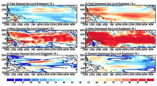
To extract the seasonal variation, a 6–18-month band-pass filter is performed in this section. The sea level variations exhibit significant spatial differences in the TPO (Figure 1a). The region with the most dramatic seasonal sea level variations is located near Clipperton Island (10.33°N, 109.22°W) in the northeastern TPO, with variances up to 50 cm2. There is also a narrow and long eastward latitude zone from 170°W between 5° and 15°N, with variances of 30–45 cm2. Additionally, seasonal sea level variations in the East Philippines (5°–15°N, 120°–128°E) and the Coral Sea (18°–13°S, 145°–165°E) are significant, with variances greater than 20 cm2. Overall, the seasonal variation amplitude of other regions of the Tropical Pacific is small, with variances of less than 10 cm2. Using Equation (1), we quantitatively evaluate the contributions of the seasonal sea level variations to the monthly mean sea level variations (Figure 1). Seasonal sea level variations across the long and narrow latitude zone between 5° and 15°N in the northern TPO explains 40–60% of the monthly mean sea level variations (Figure 1b). In most northwest and southwestern TPO regions, seasonal signals contribute 35% to 50% of the monthly mean sea level. While in the southeastern TPO, the proportion of seasonal sea level variations is relatively smaller (<15%).
To explore the contribution of the steric effect and the dynamic process to the seasonal sea level variations in the TPO (Figure 2), we use Equation (1) to calculate the influence of the steric effect and the dynamic process on sea level variations (Figure 2). The steric sea level is calculated using Equation (5), and the dynamic sea level is simulated by a 1.5-layer reduced gravity model.
Seasonal sea level variations in the TPO mainly result from the steric effect [21], especially in the central and eastern TPO, where the steric effect contributes to more than 90% of the seasonal sea level variations (Figure 2a). For the northernmost and southeastern Tropical Pacific, the contribution of the steric effect is small, even indicating a negative contribution. The dynamic process mainly acts on two long and narrow latitude zones in the northernmost central Tropical Pacific, contributing 55–85% (Figure 2b). While in most other regions of the TPO, the contribution of the dynamic process is less than 50%, and in some regions even revealing a significant negative contribution. Compared with the steric effect, the contribution of the dynamic process in the TPO is significantly weaker; therefore, the steric effect is the dominant process influencing seasonal sea level variations in the TPO. This is consistent with the previous conclusion that the steric effect plays a leading role [25].
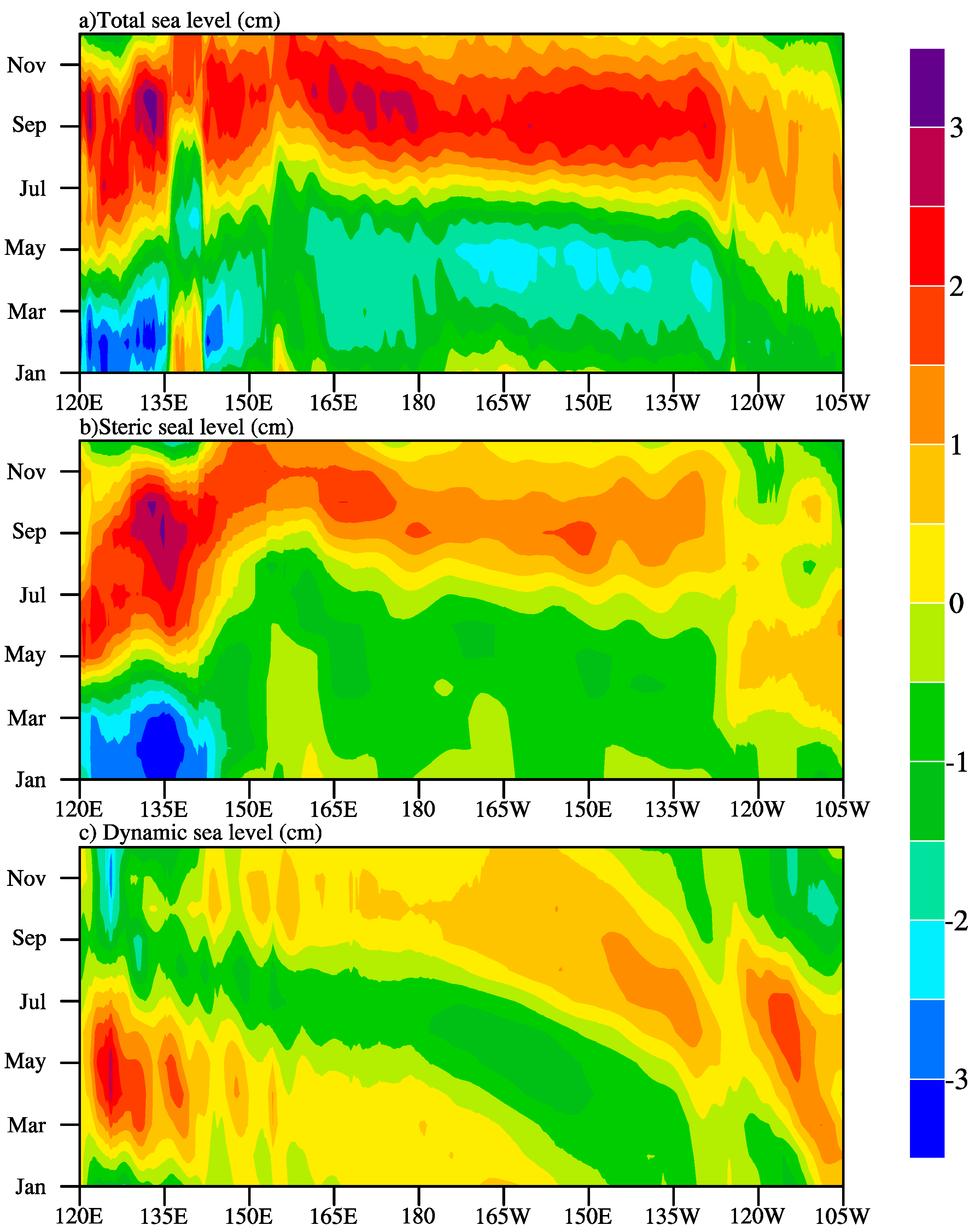
Figure 3a reveals the time–longitude features of seasonal sea level anomalies averaged from 20°S–20°N in the TPO. Positive sea level anomalies generally appear from June to December, spanning the entire TPO in the meridian direction. In the western TPO, the sea level anomalies start to appear in May, with the maximum positive sea level anomalies (>3 cm) appearing in the eastern Philippines 130°–135°E. This is distinct to the eastern TPO, where the sea level anomalies are relatively small (<1.5 cm). In other regions of TPO, especially in the west, the sea level reveals negative anomalies, with the greatest occurring from January to March, even exceeding −3 cm. The TPO is bounded by June, with negative sea level anomalies occurring before June and positive sea level anomalies after. Seasonal sea level variations propagate from west to east in the central and eastern TPO (Figure 3a), mainly caused by the steric effect, which is induced by the baroclinic Rossby waves, which in turn are driven by wind stress (Figure 3b). It is worth noting that in the meridional direction of 135°–140°E, the sea level variations are abnormal, likely resulting from variances of seasonal variations between Australia and New Guinea reaching more than 50 cm2. As this geographical location is closed, sea level variations are mainly affected by tropical cyclones, and the occurrence of tropical cyclones is closely related to the monsoon [59,60].
To explore the influence of the steric effect and the dynamic process on seasonal sea level variations in the TPO and their temporal and spatial variations, we calculated the steric sea level anomalies based on Equation (5) (Figure 3b) and the dynamic sea level anomalies simulated by a 1.5-layer reduced gravity model (Figure 3c). The spatial distribution of the steric sea level variations presents a structure similar to the altimeter sea level variations, indicating that the steric variations suitably capture the characteristics of the altimeter variations. The sea level anomalies are only minor in the middle east of the TPO (<2 cm). However, the steric sea level variations between 135°E and 140°E are completely different from the altimeter variations, confirming that the sea level anomalies in this area are indeed not caused by the steric effect but tropical cyclones. Secondly, the spatial distribution of the dynamic sea level variations is quite different from the structure of altimeter sea level variations. Dynamic sea level anomaly signals propagate westward in the form of baroclinic Rossby waves on the scale of seasonal variations. Concurrently, in the meridional direction of 120°E–135°W, the positive and negative sea level anomaly signals anomaly signals displayed an obvious arc-shaped trend. From west to east along the TPO, negative sea level anomalies occur earlier in the year (from September to January). Moreover, the seasonal sea level variations are dominated by the steric effect in most regions.
Conducting sensitivity experiments in specific regions is an important method for exploring the mechanisms of sea level variations. Experiments isolating only various wind fields and ignoring other factors can highlight the role of dynamic processes in sea level variations [59]. The seasonal sea level variations in the TPO are closely related to the wind forcing in the Pacific. Therefore, it is necessary to explore the relative effects on seasonal sea level variations in the TPO between the wind forcing in the TPO and other regions. Based on the above questions, we designed three sensitivity experiments (Table 1) to evaluate the relative effects of wind forcing on the seasonal sea level variations in different regions of the TPO.
On the basis of the comparison of the simulated results (Figure 4), the dynamic sea level derived from the control experiment (Exp 0) contributes the most to the seasonal sea level variations in the central northern Tropical Pacific (Figure 4). A long and narrow belt across the meridian explains more than 80% of the variance, while a second narrow belt is formed in eastern New Guinea (explaining 55–75%). Additionally, wind forcing significantly contributes to the variance (65–75%) in the Coral Sea (18°–13°S, 145°–165°E) and around Clipperton Island (10.33°N, 109.22°W). Nevertheless, the real monthly wind forcing explains approximately 25% of the variances in other regions and even reaches negative contributions in the north and southeast (Figure 4a). The local wind forcing in the TPO plays a leading role in seasonal sea level variations, through the comparison the simulated results of EXP 0 and EXP 1 (Figure 4a,b). If the subtropical north Pacific models the real monthly wind field, and TPO is the climatic wind field (Figure 4c), the contribution of the subtropical north Pacific wind field to seasonal sea level variations is generally consistent with the NPO wind field. Still, the variances are generally minor, with a maximum of only 75%, forming a long and narrow belt. The variances of the coral region are less than 55%, and the area of the negative contribution region in the north and southeast region expanded. This indicates that compared with the contribution of TPO wind forcing to seasonal sea level variations, the contribution of subtropical north Pacific Ocean wind forcing is relatively small. Overall, on seasonal time scales, the dynamic sea level variations in the TPO are caused by the combined effects of local wind forcing and subtropical north Pacific Ocean wind forcing, of which local wind forcing plays a leading role.
4. Interannual to Decadal Sea Level Variations in the TPO
4.1. Interannual Sea Level Variations in the TPO
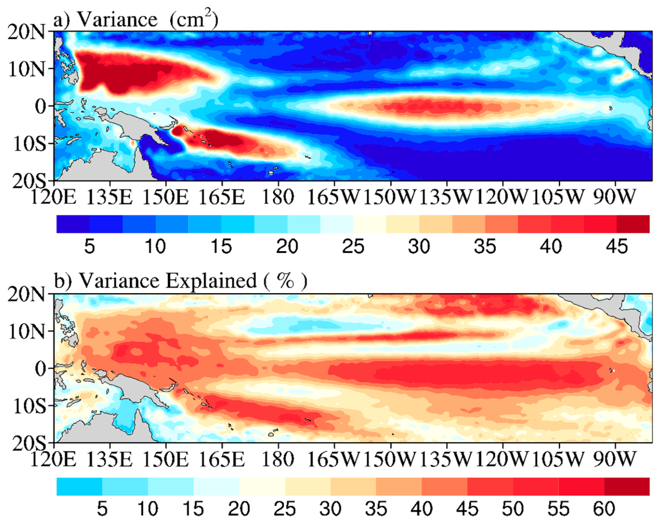
There are significant spatial differences in the interannual sea level variations in the TPO (Figure 5a). Significant interannual variations are presented in the northwest, southwest, and east-central parts of the TPO. These variances exceed 40 cm2, with the maximum value in the northwest and southwest regions surpassing 45 cm2 (Figure 5a). In these regions with high sea level interannual variation variances, the contribution of the interannual sea level signals to the monthly mean variations is as high as 45–60% (Figure 5b), and their spatial patterns are consistent with the interannual sea level variations. However, it is worth noting that the significant interannual sea level variations in the equatorial eastern Pacific can be explained by the interannual response of Kelvin waves caused by wind anomalies (Figure 5a). Variances of the interannual sea level variations are lower in other regions, less than 20 cm2 (Figure 5a). Except for the northeastern TPO, the contribution of the interannual signals to the monthly mean variations remains relatively minor (below 45%) (Figure 5b). In the northeastern TPO, while the interannual sea level variations are not large (Figure 5a), their contribution to monthly mean variations explains up to 60% (Figure 5b), further indicating that the sea level variations in this region are not significant.
From the perspective of atmospheric forcing, variations in the wind field and heat flux caused variations in ocean density field and circulation. These can induce variations in heat content and other factors, in turn causing sea level variations. Therefore, the root causes of the interannual variations are the variations of the wind field and heat flux [12,29]. The contribution of the steric effect to the interannual sea level variations in the TPO is generally significant (Figure 6), as high as 95% in the central TPO. However, there is a small area of less than 15% and even a negative contribution in the northernmost and southeastern regions. The dynamic process contributes significantly (55–80%) to the interannual sea level variations in the TPO, mainly influencing the northwest, northeast, and southern regions, and contributed less (<45%) in other regions. This is consistent with the results of previous studies [12,20,41]. The contributions of the steric effect and the dynamic process to the interannual sea level variations vary. For instance, while the contribution of the dynamic process is unevenly distributed spatially, its effect in most regions exceeds 85%. Therefore, in most regions of TPO, the steric effect and the dynamic process explains the interannual sea level variations. Similar conclusions have been reflected in previous studies [19,40,54].
The interannual sea level fluctuation signals of TPO are affected by the sea surface wind forcing. The dominant contribution to interannual sea level variations in western TPO is the wind-induced first baroclinic Rossby waves [7,24,32,36]. Therefore, exploring the relative effects of wind forcing in the TPO and the wind forcing in other regions on the interannual sea level variations is necessary. The variances explained by the wind forcing in different regions from the sensitivity control experiments (Figure 7) reveal that the real monthly wind forcing contributed to the interannual sea level variations. These are larger in the northwest, south, and southwest (>65%), only reaching 65% in the northeast. However, its contribution is minor and even negative in other regions. When the TPO is modeled with the real monthly wind field, and other regions are the climatic wind fields (Figure 7b), the contribution of local wind forcing to the interannual sea level variations in the TPO is almost the same as the real wind forcing. The variances are also the same, indicating that the local wind field in the TPO plays a leading role in influencing the interannual sea level variations. However, when the subtropical north Pacific Ocean is modeled with the real monthly wind field and TPO is the climatic wind field (Figure 7c), the subtropical north Pacific Ocean wind field explains less than 15% of the variances of the interannual sea level variations. This indicates that the subtropical north Pacific wind forcing barely contributes to this region. Therefore, the local wind forcing in the TPO is the leading role of the interannual sea level variations.
4.2. Decadal Sea Level Variations in the TPO
There are significant spatial differences in decadal sea level variations in the TPO. They are most dramatic in the eastern Philippines of the northwestern TPO, with a maximum variance of more than 40 cm2. In the southwest, central, eastern, and northeastern regions, these variances range from 10 cm2 to 20 cm2, and are generally lower in other regions (<10 cm2) (Figure 8a). The contribution of decadal signals to monthly mean sea level variations in the northeastern and southeastern TPO is as high as 50–70%, with some regions exceeding 70% (Figure 8b). Decadal contributions are the smallest in the north-central and southwestern regions, as low as 25% (Figure 8b). The spatial characteristics of the contribution of decadal signals to monthly mean sea level variations are quite different from those of decadal sea level variations.
The decadal sea level variations in the TPO are mainly controlled by large-scale ocean–atmosphere processes such as PDO and the decadal variations of ENSO [53,61]. ENSO and PDO primarily affect sea level variations through variations in trade winds in the Pacific Ocean, alongside numerous other factors, such as the effect of heat flux and so on [29]. Similar to the interannual time scales, on decadal time scales, the contribution of the hematocrit effect to the sea level variations in the TPO is dominant, and the maximum contribution exceeds 95% (Figure 9). At the same time, the dynamic process mainly acts on the northwestern and southwestern of the TPO, which is consistent with previous studies [62], with contributions of approximately 55–70%. While the contribution of the dynamic process is generally lower in the eastern TPO, it is mainly dominated by the steric effect (Figure 9). There are considerable differences between the steric effect and the intensity of the dynamic process, i.e., the dynamic process only contributed more than the steric in the central and western areas, and its greatest contribution is no more than 65%. In the central and western regions of TPO, the combined effect of the hematocrit effect (major contributor) and dynamic process explains 100% of the decadal sea level variations.
The decadal signals are mainly driven by wind stress in the TPO. Abnormal wind stress and wind stress curl are considered to be the leading causes of sea level variations in the TPO on interannual and decadal scales [32,53,54,55]. Therefore, it is necessary to explore the relative effect of wind forcing in different regions of the Pacific Ocean on the sea level variations in the TPO. The contribution of real monthly wind forcing to the decadal sea level variations in the TPO is greater in the northwest and southwest regions (>65%) (Figure 10). The contribution in other regions is minor and in some regions it is even negative. If TPO models the real monthly wind field and other regions include the climatic wind fields (Figure 10b), the contribution of local wind forcing in the TPO to the decadal sea level variations is almost the same as the real wind forcing. Furthermore, the variances of the variations were almost the same, revealing that the local wind forcing in the TPO plays a significant role in the decadal sea level variations. If the subtropical north Pacific Ocean includes the real monthly wind field and TPO is the climatic wind field (Figure 10c), then the wind field of subtropical north Pacific contributes little or even negatively to the decadal sea level variations in most regions of the TPO. Therefore, local wind forcing in the TPO is likely the leading role of the decadal sea level variations.
4.3. Interannual to Decadal Sea Level Variations in the TPO
The eastern and western TPO has recently exhibited a seesaw spatial pattern of annual mean sea level anomalies (Figure 11a). Sea level anomalies and negative sea level anomalies alternately appeared during 1993–1995, especially when ENSO occurred. Negative anomalies (blue) occurred during El Niño: 1997, 1997, 2002–2005, 2007, 2014–2016, and 2018–2019. On the contrary, positive anomalies (red) occurred during La Niña: 1996, 1998–2001, 2008–2013, and 2017 (Figure 11a). The meridional mean sea level anomalies in the TPO are significant (>3 cm or <−3 cm), and mainly concentrates in a small latitude zone, roughly between 120°E–140°E in the eastern Philippines (5°–15°N, 120°–128°E) and western New Guinea (10°S–0°, 135°–150°E). The eastward signals gradually weaken, while the negative sea level anomalies form in a long and narrow belt along the zonal direction. This phenomenon also confirms that the interannual sea level variations in the TPO and its low-frequency modulation are driven by ENSO [32,33,36,61]. It is worth noting that from the entire time–longitude diagram, the sea level anomalies in the TPO have the characteristics of an east–west reverse-phase variation in the zonal direction of west longitude 170°W. In contrast to this region, this phenomenon is consistent with the results of previous studies [42,62,63].
The sea level variations induced by the steric effect strongly reflect the characteristics of the altimeter sea level variations. Its spatial distribution presents a structure similar to the altimeter sea level variations, which is driven by ENSO (Figure 11), which indicates that the steric sea level variations have a dominant effect on the altimeter sea level variations. At the same time, the spatial pattern of the low-frequency dynamic sea level variations in the latitude 165°E–135°W region is roughly the same as the altimeter sea level variations. However, the magnitude of the variations is small, indicating that the dynamic sea level variations affect the low-frequency altimeter sea level variations. The dynamic process mainly involves the interannual to decadal sea level variations in the TPO through the westward propagation of Rossby waves (Figure 11c). Therefore, similar to the sea level variations from interannual to decadal time scales, the steric effect and the dynamic process works together to influence the sea level variations in the TPO, with the steric effect being dominant.
4.4. Interannual and Decadal Sea Level Fingerprints of TPO
The contribution of the PDO to sea level variations can be inferred from the increase of the sea level climate index. Based on the PDO index and Multivariate ENSO Index (MEI), using multiple regression methods, Zhang and Church (2012) defined new interannual and decadal climate indexes to explain the low-frequency sea level variations in the Pacific Ocean since 1993. They concluded that 60% of the observed low-frequency sea level variations originated from internal climate models (ENSO and PDO) [64].
Therefore, in order to explore the impact of ENSO and PDO on sea level variations in the TPO, we used the multiple regression model (MVLR) to simulate the interannual and decadal sea level fingerprints of TPO (Figure 12a,b). The annual sea level fingerprint is expressed as the regression of sea level relative to ICI, equivalent to the regression coefficient a1 in Equation (2) and closely related to ENSO. For the interannual sea level fingerprint, the regions with the most significant regression results are western and eastern TPO. The maximum interannual sea level fingerprint reaches 80 mm/unit ICI in the eastern regions, and the largest in the western sea is −80 mm/unit ICI; this spatial feature is similar to a “seesaw”. During El Niño Taimasa, the abnormal movement of the zonal wind and the corresponding wind stress curl lead to the “seesaw” pattern of the sea level of TPO, manifesting as sea level rise in the eastern TPO and a decline in the warm pool area (10°S–10°N, 60°W–150°E). In the northwest and southeastern TPO, the sea level meridional seesaw mode with 5°N as the fulcrum is also related to the air–sea coupling mode [30,65,66,67]. Secondly, we used Equation (1) to calculate the contribution of ENSO-related sea level variations to interannual to decadal sea level variations (Figure 12c), which corresponded to the interannual sea level fingerprint. In the eastern and western regions of the TPO, ENSO-related sea level variation explanation reaches more than 65%, while the variance in the north American coast reached 60%. The contribution of ENSO in the regions near the C-shaped east–west boundary of the “seesaw” is low, less than 10%. Therefore, the ENSO can better explain the interannual sea level variations in the western and eastern TPO and the coast of north America. The interannual sea level fingerprint and the spatial characteristics of its contribution are consistent with the impact of the ENSO dynamic on the interannual sea level variations in the TPO [31,68].
In addition, we used Equation (1) to calculate the decadal sea level fingerprint as the regression of sea level with respect to DCI, which is equivalent to the regression coefficient a2 in Equation (2) (closely related to PDO). For the decadal sea level fingerprint, the most significant region of the regression result is located in the northwest TPO, namely the eastern Philippines, with a maximum of −80 mm/unit DCI. In addition, the regions with more significant variations include the eastern and northeastern regions of the Pacific Ocean. The north American coast ranges between 40–70 mm/unit DCI, and the “seesaw” structure is no longer apparent compared with the interannual sea level fingerprint (Figure 12b). We used Equation (1) to calculate the contribution of PDO-related sea level variations to the interannual to decadal altimeter sea level variations (Figure 12d), which strongly corresponds to the decadal sea level fingerprint. The regions in the narrow and long latitudes with high contributions contribute more than 60%, and the contribution in the northwestern region is between 35–50%. In comparison, it contributes less than 40% in all other regions, indicating that PDO can better explain the interannual to decadal sea level variations only in the northwest and northeast TPO.
From the perspective of interannual sea level fingerprint, decadal sea level fingerprint, and their respective contributions to sea level variations, the combined effect of ENSO and PDO can explain 100% of the interannual to decadal sea level variations in the northwest and East TPO. For the coast of north America, the contribution of ENSO and PDO can explain more than 90%. In the southwestern TPO, the joint action of ENSO and PDO has little impact on the interannual to decadal sea level variations in this region. The low-frequency sea level variations in this region are dominated by the steric effect and other processes (Figure 6a, Figure 7a, Figure 9a, Figure 10a).
5. Summary and Discussion
5.1. Discussion
The quantitative analysis results of the influence of wind field and heat steric factors on sea level variations have many interannual scales and a relative lack of decadal scales. The length and quality of the data are the key factors that affect the quantitative analysis of sea level variations in the TPO [29]. The satellite altimeter data, thermohaline data, and model data used in this paper span only 27 years, which is insufficient to study decadal sea level variations. Secondly, substantially different sources of wind field data and temperature and salt data are also reasons for the above problems. In addition, the dynamic sea level simulated by the 1.5-layer reduced gravity model is only driven by the wind field. The simulation is not the real dynamic sea level due to the lack of real terrain and stratification. Therefore, it is necessary for a high-precision three-dimensional ocean numerical model to quantitatively compare the effect of different wind forcing in future research. Finally, although the method estimates the magnitude of interannual to decadal sea level variations associated with ENSO, the regression was based on a limited time frame spanning only a few ENSO events. With the continuous growth of time series, the regression amplitude could be improved.
5.2. Summary
In this paper, we used satellite altimeter data, temperature and salinity data, and the 1.5-layer reduced gravity model to analyze the characteristics of the sea level temporal and spatial variations in the TPO and quantitatively assess the contribution of the steric effect and the dynamic process to sea level variations at different time scales. At the same time, we also discuss the impact of wind forcing in different regions on sea level variations in the TPO. Based on a multiple regression model, we quantified the relative contribution of interannual variations related to ENSO and decadal variations related to PDO to low-frequency sea level variations in the TPO. The sea level variations in the TPO exhibit significant multi-timescale variations [15,16,17,18]. Seasonally, the meridional mean sea level of TPO produces negative anomalies from January to May and positive anomalies from June to December. The steric sea level variations are the same as the satellite altimeter sea level variations. In contrast, the dynamic sea level propagates westward from the eastern Pacific Ocean, distinct from the altimeter sea level. In terms of the spatial distribution, the sea level variations are most significant in the long and narrow latitude zone from 170°W eastward between 5° and 15°N, with a variance range of 30–50 cm2, explaining 40–60% of the monthly variations. Secondly, it is also more evident in the southeastern and southwestern regions of the Tropical Pacific 30–50 cm2. The seasonal sea level variations range from 10–40 cm2 and explained 35–45% of the monthly mean sea level variations. The steric effect and the dynamic process together influences the seasonal sea level variations in the TPO. Among them, the steric effect is dominant, and the contribution in most regions exceeds 70%. The dynamic process mainly affects the regions on both sides of the equator and the southwestern TPO. The contribution of this region is about 55–85%. Concurrently, the dynamic sea level variations are induced by the combined effect of the local wind forcing and the subtropical north Pacific Ocean wind forcing, of which the local wind forcing plays a leading role.
On the interannual time scales, the eastern and western TPO exhibits a seesaw spatial pattern during ENSO. During the El Niño period, the sea level in the eastern Pacific Ocean presented positive anomalies, and the sea level in the western Pacific Ocean presented negative anomalies. The opposite is the case during the La Niña period. The sea level anomalies are consistent with the altimeter sea level anomalies in changeable amplitude and phases. The dynamic process mainly affects the interannual sea level variations in the central and eastern TPO through the westward propagation of Rossby waves. At the same time, there are significant spatial differences in the interannual sea level variations in the TPO. The interannual variations are most significant in the northwest, southwest, and central and eastern regions of TPO, with a variance of more than 40 cm2. The interannual sea level variations vary from month to month, while the contribution of the mean sea level variations is as high as 45–60%. The steric effect and the dynamic process strongly explains the interannual sea level variations in the TPO. Among them, the steric effect contributes relatively higher, up to 95% near the equator, to the interannual sea level variations in the TPO. The influence of the dynamic process is mainly concentrated in the northwest, northeast, and southern regions of the TPO, and its contribution is about 55–80%. The local wind forcing in the TPO is the dominant influence on interannual sea level variations, and the contribution of wind forcing in other regions is small or even negative.
On the decadal time scales, sea level variations in the TPO are mainly controlled by large-scale ocean–atmosphere processes such as PDO and the decadal variations of ENSO [29]. The region with the most dramatic decadal sea level variations in the TPO is located in the northwestern region of the eastern Philippines, and its variance exceeds 40 cm2. This area can explain 25–45% of the monthly mean sea level variations. The regions with the greatest contribution to the monthly mean sea level variations are in the southeast and northwest, 50–70%. The steric effect and the dynamic process explained 100% of the decadal sea level variations in most regions of the TPO. The region near the equator mainly contributed more than 85% of the steric effect. The dynamic process primarily acts on the southwest and northwest regions of the TPO, contributing only about 55–70% in others. The local wind forcing in the TPO is the leading role of decadal sea level variations. The contribution of wind forcing in other regions is small or even negative.
The most significant regions with interannual and decadal sea level fingerprints in the TPO are located in the western and central-eastern regions of TPO, with their maximum reaching 80 mm/unit ICI and 80 mm/unit DCI. The combined effect of ENSO and PDO explains 100% of the interannual to decadal sea level variations in the northwestern and eastern TPO. For the coast of north America, ENSO and PDO explained more than 90%. In the southwestern TPO, the combined effect of ENSO and PDO has minimal effect on the interannual to decadal sea level variations. The process that dominated this region’s low-frequency sea level variations is mainly the steric effect and other processes.
Author Contributions
J.L. proposed the idea. J.W. collected data and made the analysis. J.L. and J.Y. wrote the manuscript. W.T. and Y.L. helped the data preparation and participated in discussions on the results. All authors have read and agreed to the published version of the manuscript.
Funding
This work was funded by National Natural Science Foundation of China (42006021, 41806039, 42076233, 41806004).
Institutional Review Board Statement
Not applicable.
Informed Consent Statement
Not applicable.
Data Availability Statement
All the data links can be found in Section 2.1.
Acknowledgments
The satellite altimeter data is maintained and provided by Archiving, Validation, and Interpretation of Satellite Oceanographic center, with support from the AVISO (ftp://ftp-access.aviso.altimetry.fr/climatology, accessed on 22 September 2021). We acknowledge the anonymous reviewers. The authors would like to express their gratitude to EditSprings (https://www.editsprings.cn/, accessed on 22 September 2021) for the expert linguistic services provided.
Conflicts of Interest
The authors declare they have no conflict of interest.
References
- Hallegatte, S.; Green, C.; Nicholls, R.J.; Corfee-Morlot, J. Future flood losses in major coastal cities. Nat. Clim. Chang. 2013, 3, 802–806. [Google Scholar] [CrossRef]
- Wong, P.P.; Losada, I.J.; Gattuso, J.P.; Hinkel, J.; Khattabi, A.; McInnes, K.L.; Saito, Y.; Sallenger, A. Climate Change 2014—Impacts, Adaptation, and Vulnerability. Part A: Global and Sectoral Aspects. Contribution of Work-ing Group II to the Fifth Assessment Report of the Intergovernmental Panel on Climate Change. In Coastal Systems and Low–Lying Areas; Field, C.B., Barros, V.R., Dokken, D.J., Mach, K.J., Mastrandrea, M.D., Bilir, T.E., Chatterjee, M., Ebi, K.L., Estrada, Y.O., Genova, R.C., et al., Eds.; Cambridge University Press: Cambridge, UK, 2014; pp. 361–409. [Google Scholar]
- Church, J.A.; White, N.J. Sea-level rise from the late 19th to the early 21st century. Surv. Geophys. 2011, 32, 585–602. [Google Scholar] [CrossRef] [Green Version]
- Becker, M.; Meyssignac, B.; Letetrel, C.; Llovel, W.; Cazenave, A.; Delcroix, T. Sea level variations at tropical Pacific islands since 1950. Glob. Planet. Chang. 2011, 80, 85–98. [Google Scholar] [CrossRef]
- Zhang, X.B.; Church, J.A. Sea level trends, interannual and decadal variability in the Pacific Ocean. Geophys. Res. Lett. 2012, 39. [Google Scholar] [CrossRef]
- Merrifield, M.A.; Mathew, E.M. Regional sea level trends due to a Pacific trade wind intensification. Geophys. Res. Lett. 2011, 38. [Google Scholar] [CrossRef]
- Qiu, B.; Chen, S.; Wu, L.; Kida, S. Wind- versus eddy-forced regional sea level trends and variability in the North Pacific Ocean. J. Clim. 2015, 28, 1561–1577. [Google Scholar] [CrossRef]
- Axel, M.; Mikael, C.; David, A.T.H.; Thomas, S. Ordovician and Silurian sea–water chemistry, sea level, and climate: A synopsis. Palaeogeogr. Palaeoclimatol. Palaeoecol. 2010, 296, 389–413. [Google Scholar] [CrossRef]
- Merrifield, M.A.; Thompson, P.R.; Lander, M. Multidecadal sea level anomalies and trends in the western tropical Pacific. Geophys. Res. Lett. 2012, 39. [Google Scholar] [CrossRef]
- Chen, D.; Cane, M.A.; Zebiak, S.E.; Kaplan, A. The impact of sea level data assimilation on the Lamont Model Prediction of the 1997/98 El Niño. Geophys. Res. Lett. 1998, 25, 2837–2840. [Google Scholar] [CrossRef]
- Chambers, D.P.; Chen, J.; Nerem, R.S.; Tapley, B.D. Interannual mean sea level change and the Earth’s water mass budget. Geophys. Res. Lett. 2000, 27, 3073–3076. [Google Scholar] [CrossRef]
- Christopher, G.P.; Rui, M.P. Buoyancy-driven interannual sea level changes in the southeast tropical pacific. Geophys. Res. Lett. 2012, 39. [Google Scholar] [CrossRef]
- Li, L.; Xu, J.; Cai, R.S. Trends of sea level rise in the South China Sea during the 1990s: An altimetry result. Chin. Sci. Bull. 2013. [Google Scholar] [CrossRef]
- Cazenave, A.; Llovel, W. Contemporary Sea Level Rise. Annu. Rev. Mar. Sci. 2010, 2, 145–173. [Google Scholar] [CrossRef] [Green Version]
- Anny, C.; Frédérique, R. Sea level and climate: Measurements and causes of changes. Wiley Interdiscip. Rev. Clim. Chang. 2011, 2, 647–662. [Google Scholar] [CrossRef]
- Merrifield, M.A. A Shift in Western Tropical Pacific Sea Level Trends during the 1990s. J. Clim. 2011, 24, 4126–4138. [Google Scholar] [CrossRef]
- Han, W.Q.; Meehl, G.A.; Hu, A.X.; Alexander, M.A.; Yamagata, T.; Yuan, D.L.; Ishii, M.; Pegion, P.; Zheng, J.; Hamlington, B.D.; et al. Intensification of decadal and multi-decadal sea level variability in the western tropical Pacific during recent decades. Clim. Dyn. 2014, 43, 1357–1379. [Google Scholar] [CrossRef]
- Hu, S.J.; Fu, D.Y.; Han, Z.L.; Ye, H. Density, Demography, and Influential Environmental Factors on Overwintering Populations of Sogatella furcifera (Hemiptera: Delphacidae) in Southern Yunnan, China. J. Insect Sci. 2015, 15, 58. [Google Scholar] [CrossRef] [Green Version]
- Lu, Q.; Zuo, J.C.; Wu, L.J. Low-frequency variation in sea level in the tropical Pacific. Haiyang Xuebao 2017, 39, 43–52. [Google Scholar] [CrossRef]
- Lu, Q.; Zuo, J.C.; Li, Y.F.; Chen, M.X. Interannual sea level variability in the tropical Pacific Ocean from 1993 to 2006. Glob. Planet. Chang. 2013, 107, 70–81. [Google Scholar] [CrossRef]
- Chen, J.L.; Shum, C.K.; Wilson, C.R.; Chambers, D.P.; Tapley, B.D. Seasonal sea level change from TOPEX/Poseidon observation and thermal contribution. J. Geod. 2000, 73, 638–647. [Google Scholar] [CrossRef]
- Yu, H.L. The characteristic of Northwest Pacific sea level variation, and influencing factor. J. Ocean. Univ. China 2013, 43, 9–20. [Google Scholar] [CrossRef]
- Li, X.H.; Wei, G.J.; Shao, L.; Liu, Y.; Liang, X.R.; Jian, Z.M.; Sun, M.; Wang, P.X. Geochemical and Nd isotopic variations in sediments of the South China Sea: A response to Cenozoic tectonism in SE Asia. Earth Planet. Sci. Lett. 2003, 211, 207–220. [Google Scholar] [CrossRef]
- Li, J.; Tan, W.; Chen, M.X.; Luo, F.Y.; Liu, Y.; Fu, Q.J.; Li, B.T. An extreme sea level event along the northwest coast of the South China sea in 2011–2012. Cont. Shelf Res. 2020, 196, 104073. [Google Scholar] [CrossRef]
- Busalacchi, A.J.; Mcphaden, M.J.; Picaut, J.; Springer, S.R. Sensitivity of wind-driven tropical Pacific Ocean simulations on seasonal and interannual time scales. J. Mar. Syst. 1990, 1, 119–154. [Google Scholar] [CrossRef]
- Sergey, V.; Vinogradov, R.M.; Ponte, P.H.; Carl, W. The mean seasonal cycle in sea level estimated from a data-constrained general circulation model. J. Geophys. Res. Ocean. 2008, 113. [Google Scholar] [CrossRef]
- Roberts, C.D.; Calvert, D.; Dunstone, N.; Hermanson, L.; Palmer, M.D.; Smith, D. On the Drivers and Predictability of Seasonal-to-Interannual Variations in Regional Sea Level. J. Clim. 2016, 29, 7565–7585. [Google Scholar] [CrossRef]
- Chen, X.; Qiu, B.; Cheng, X.H.; Qi, Y.Q.; Du, Y. Intra-seasonal variability of Pacific-origin sea level anomalies around the Philippine Archipelago. J. Oceanogr. 2015, 71, 239–249. [Google Scholar] [CrossRef]
- Chen, M.X.; Zuo, C.S.; Zhang, W.H.; Jia, Y.R.; Lyu, X.F. Research progress of inter-annual and multi-decadal sea level variability in tropical Pacific Ocean. J. Oceanogr. 2017, 45, 249–255. [Google Scholar] [CrossRef]
- Chang, Y.T.; Du, L.; Zhang, S.W.; Huang, P.F. Sea level variations in the tropical Pacific Ocean during two types of recent El Niño events. Glob. Planet. Chang. 2013, 108, 119–127. [Google Scholar] [CrossRef]
- Landerer, F.W.; Jungclaus, J.H.; Marotzke, J. El Niño–Southern Oscillation signals in sea level, surface mass redistribution, and degree-two geoid coefficients. J. Geophys. Res. Ocean. 2008, 113, C08014. [Google Scholar] [CrossRef] [Green Version]
- Wang, G.Q.; Jin, J.L.; Wan, S.C.; Zhai, R. Variation of sea level rise along the China coastal area during the past decades. In Proceedings of the 2015 Academic Annual Meeting of China Water Conservancy Society, Nanjing, China, 26–28 October 2015; Volume II. [Google Scholar]
- Li, L.H.; Zhou, L.H.; Lian, H.J. Sea-level Rise Forecast Model. J. Comput. 2011, 6, 2120–2126. [Google Scholar] [CrossRef]
- Han, W.Q.; Gerald, A.; Meehl, A.; Detlef, S.; Aixue, H.; Benjamin, H.; Jessica, K.; Hindumathi, P.; Philip, T. Spatial Patterns of Sea Level Variability Associated with Natural Internal Climate Modes. Surv. Geophys. 2017, 38, 221–254. [Google Scholar] [CrossRef] [Green Version]
- Meng, L.S.; Zhuang, W.; Zhang, W.W.; Ditri, A.; Yan, X.H. Decadal Sea Level Variability in the Pacific Ocean: Origins and Climate Mode Contributions. J. Atmos. Ocean. Technol. 2019, 36, 689–698. [Google Scholar] [CrossRef]
- Duan, J.; Li, Y.L.; Zhang, L.; Wang, F. Impacts of the Indian Ocean Dipole on Sea Level and Gyre Circulation of the Western Tropical Pacific Ocean. J. Clim. 2020, 33, 4207–4228. [Google Scholar] [CrossRef] [Green Version]
- Merrifield, M.; Kilonsky, B.; Nakahara, S. Interannual sea level changes in the tropical Pacific associated with ENSO. Geophys. Res. Lett. 1999, 26, 3317–3320. [Google Scholar] [CrossRef]
- Nerem, R.S.; Chambers, D.P.; Choe, C.; Mitchum, G.T. Estimating Mean Sea Level Change from the TOPEX and Jason Altimeter Missions. Mar. Geod. 2010, 33, 435–446. [Google Scholar] [CrossRef]
- Long, X.Y.; Widlansky, M.J.; Schloesser, F.; Thompson, P.R.; Annamalai, H.; Merrifield, M.A.; Yoon, H. Higher Sea Levels at Hawaii Caused by Strong El Niño and Weak Trade Winds. J. Clim. 2020, 33, 3037–3059. [Google Scholar] [CrossRef]
- Fu, L.; Qiu, B. Low-frequency variability of the North Pacific Ocean: The roles of boundary- and wind-driven baroclinic Rossby waves. J. Geophys. Res. Ocean. 2002, 107, 3220. [Google Scholar] [CrossRef]
- Zhuang, W.; Qiu, B.; Du, Y. Low-frequency western Pacific Ocean sea level and circulation changes due to the connectivity of the Philippine archipelago. J. Geophys. Res. 2013, 118, 6759–6773. [Google Scholar] [CrossRef]
- Qiu, B.; Chen, S. Interannual-to-Decadal Variability in the Bifurcation of the North Equatorial Current off the Philippines. J. Phys. Oceanogr. 2010, 40, 2525–2538. [Google Scholar] [CrossRef]
- Mantua, N.J.; Hare, S.R.; Zhang, Y.; Wallace, J.M.; Francis, R.C. A Pacific interdecadal climate oscillation with impacts on salmon production. Bull. Am. Meteorol. Soc. 1997, 78, 1069–1079. [Google Scholar] [CrossRef]
- Wu, B.Y.; Wang, J. Winter Arctic oscillation, Siberian high and East Asian winter monsoon. Geophys. Res. Lett. 2002, 29, 1897. [Google Scholar] [CrossRef]
- Feng, W.; Zhong, M.; Xu, H.Z. Sea level variation in the South China Sea inferred from satellite gravity, altimetry, and oceanographic data. Sci. China Earth Sci. 2012, 55, 1696–1701. [Google Scholar] [CrossRef]
- Peng, D.J.; Palanisamy, H.; Cazenave, A.; Meyssignac, B. Interannual Sea Level Variations in the South China Sea Over 1950–2009. Mar. Geod. 2013, 36, 164–182. [Google Scholar] [CrossRef]
- Wu, L.L.; Wang, X.L.L.; Yang, F. Historical wave height trends in the South and East China Seas, 1911-2010. J. Geophys. Res. Ocean. 2014, 119, 4399–4409. [Google Scholar] [CrossRef]
- Zhou, J.; Li, P.L.; Yu, H.L. Characteristics and mechanisms of sea surface height in the South China Sea. Glob. Planet. Chang. 2012, 88, 20–31. [Google Scholar] [CrossRef]
- Deng, W.F.; Wei, G.J.; Xie, L.H.; Ke, T.; Wang, Z.B.; Zeng, T.; Liu, Y. Variations in the Pacific Decadal Oscillation since 1853 in a coral record from the northern South China Sea. J. Geophys. Res. Ocean. 2013, 118, 2358–2366. [Google Scholar] [CrossRef] [Green Version]
- Han, S.L. Estimation of extreme sea levels along the Bangladesh coast due to storm surge and sea level rise using EEMD and EVA. J. Geophys. Res. Ocean. 2013, 118, 4273–4285. [Google Scholar] [CrossRef]
- Church, J.A.; White, N.J.; Hunter, J.R. Sea-level rise at tropical Pacific and Indian Ocean islands. Glob. Planet. Chang. 2006, 53, 155–168. [Google Scholar] [CrossRef]
- Nidheesh, A.G.; Lengaigne, M.; Vialard, J.; Izumo, T.; Unnikrishnan, A.S.; Meyssignac, B.; Hamlington, B.; Boyer Montegut, C. Robustness of observation-based decadal sea level variability in the Indo-Pacific Ocean. Geophys. Res. Lett. 2017, 44, 7391–7400. [Google Scholar] [CrossRef] [Green Version]
- Moon, J.; Song, Y.T.; Lee, H.K. PDO and ENSO modulations intensified decadal sea level variability in the tropical Pacific. J. Geophys. Res. Ocean. 2015, 120, 8229–8237. [Google Scholar] [CrossRef]
- Deepa, J.S.; Gnanaseelan, C.; Mohapatra, S.; Chowdary, J.S.; Karmakar, A.; Kakatkar, R.; Parekh, A. The Tropical Indian Ocean decadal sea level response to the Pacific Decadal Oscillation forcing. Clim. Dyn. 2019, 52, 5045–5058. [Google Scholar] [CrossRef]
- Deepa, J.S.; Gnanaseelan, C.; Parekh, A. The sea level variability and its projections over the Indo-Pacific Ocean in CMIP5 models. Clim. Dyn. 2021, 57, 173–193. [Google Scholar] [CrossRef]
- Piecuch, C.G.; Thompson, P.R.; Ponte, R.M.; Merrifield, M.A.; Hamlington, B.D. What Caused Recent Shifts in Tropical Pacific Decadal Sea-Level Trends? J. Geophys. Res. Ocean. 2019, 124, 7575–7590. [Google Scholar] [CrossRef]
- Hu, Z.Z.; Kumar, A.; Ren, H.L.; Wang, H.; L’Heureux, M.; Jin, F.F. Weakened Interannual Variability in the Tropical Pacific Ocean since 2000. J. Clim. 2013, 26, 2601–2613. [Google Scholar] [CrossRef]
- Thomson, R.E.; Tabata, S. Steric height trends at Ocean Station PAPA in the northeast Pacific Ocean. Mar. Geod. 1987, 11, 103–113. [Google Scholar] [CrossRef]
- Gharineiat, Z.; Deng, X.L. Description and assessment of regional sea-level trends and variability from altimetry and tide gauges at the northern Australian coast. Adv. Space Res. 2018, 61, S0273117718301984. [Google Scholar] [CrossRef] [Green Version]
- Nidheesh, A.G.; Lengaigne, M.; Vialard, J.; Unnikrishnan, A.S.; Dayan, H. Decadal and long-term sea level variability in the tropical Indo-Pacific Ocean. Clim. Dyn. 2013, 41, 381–402. [Google Scholar] [CrossRef]
- Wyrtki, K. Investigation of the EI Nino Phenomenon in the Pacific Ocean. Environ. Conserv. 1975, 2, 281. [Google Scholar] [CrossRef]
- Li, S.; Zhao, J.; Li, Y.; Qu, P. Study on Decadal Variability of Sea Surface Height in the Tropical Pacific Ocean. Adv. Mar. Sci. 2008. [Google Scholar] [CrossRef]
- Zhu, Z.N.; Zhu, X.H.; Guo, X.Y. Coastal tomographic mapping of nonlinear tidal currents and residual currents. Cont. Shelf Res. 2017, 143, 219–227. [Google Scholar] [CrossRef]
- Palanisamy, H.; Cazenave, A.; Delcroix, T.; Meyssignac, B. Spatial trend patterns in the Pacific Ocean sea level during the altimetry era: The contribution of thermocline depth change and internal climate variability. Ocean. Dyn. 2015, 65, 341–356. [Google Scholar] [CrossRef]
- Matthew, J.W.; Axel, T.; Karl, S.; Shayne, M.; Niklas, S.; Matthew, H.E.; Matthieu, L.; Wenju, C. Changes in South Pacific rainfall bands in a warming climate. Nat. Clim. Chang. 2013, 3, 417–423. [Google Scholar] [CrossRef] [Green Version]
- Matthew, J.; Widlansky, A.T.; Wenju, C. Future extreme sea level seesaws in the tropical Pacific. Sci. Adv. 2015, 1, e1500560. [Google Scholar] [CrossRef] [Green Version]
- Gaël, A.; Thierry, D. Interannual sea level changes and associated mass transports in the tropical Pacific from TOPEX/Poseidon data and linear model results (1964–1999). J. Geophys. Res. Ocean. 2002, 107, 17-1–17-22. [Google Scholar] [CrossRef]
- Nerem, R.S.; Chambers, D.P.; Leuliette, E.W.; Mitchum, G.T.; Giese, B.S. Variations in global mean sea level associated with the 1997–1998 ENSO event: Implications for measuring long-term sea level change. Geophys. Res. Lett. 1999, 26, 3005–3008. [Google Scholar] [CrossRef]
Figure 1.
(a) The seasonal sea level variances and (b) explained variances in the TPO.

Figure 2.
The seasonal sea level explained variances of (a) the steric effect and (b) the dynamic process.
Figure 2.
The seasonal sea level explained variances of (a) the steric effect and (b) the dynamic process.

Figure 3.
Time–longitude plot of the seasonal sea level anomalies (cm) averaged along the 20°S–20°N latitudinal band from (a) altimetric observations, (b) the steric effect, and (c) the 1.5-layer model.
Figure 3.
Time–longitude plot of the seasonal sea level anomalies (cm) averaged along the 20°S–20°N latitudinal band from (a) altimetric observations, (b) the steric effect, and (c) the 1.5-layer model.

Figure 4.
Contributions of different wind forcing to seasonal sea level variations: (a) the real monthly wind field; (b) the real wind field in the TPO and the climatic wind field in other regions; (c) the real wind field in other regions and the climatic wind field in the TPO.
Figure 4.
Contributions of different wind forcing to seasonal sea level variations: (a) the real monthly wind field; (b) the real wind field in the TPO and the climatic wind field in other regions; (c) the real wind field in other regions and the climatic wind field in the TPO.

Figure 5.
(a) The interannual sea level variances and (b) explained variances in the TPO.

Figure 6.
The interannual sea level explained variances of (a) the steric effects and (b) the dynamic process.
Figure 6.
The interannual sea level explained variances of (a) the steric effects and (b) the dynamic process.

Figure 7.
Contributions of different wind forcing to interannual sea level variations: (a) the real monthly wind field; (b) the real wind field in the TPO and the climatic wind field in other regions; (c) the real wind field in other regions and the climatic wind field in the TPO.
Figure 7.
Contributions of different wind forcing to interannual sea level variations: (a) the real monthly wind field; (b) the real wind field in the TPO and the climatic wind field in other regions; (c) the real wind field in other regions and the climatic wind field in the TPO.

Figure 8.
(a) The decadal sea level variances and (b) explained variances in the TPO.

Figure 9.
The decadal sea level explained variances of (a) the steric effect and (b) the dynamic process.
Figure 9.
The decadal sea level explained variances of (a) the steric effect and (b) the dynamic process.

Figure 10.
Contributions of different wind forcing to decadal sea level variations: (a) the real monthly wind field; (b) the real wind field in the TPO and the climatic wind field in other regions; (c) the real wind field in other regions and the climatic wind field in the TPO.
Figure 10.
Contributions of different wind forcing to decadal sea level variations: (a) the real monthly wind field; (b) the real wind field in the TPO and the climatic wind field in other regions; (c) the real wind field in other regions and the climatic wind field in the TPO.

Figure 11.
Time–longitude plot of the interannual to decadal sea level anomalies (cm) averaged along the 20°S–20°N latitudinal band from (a) altimetric observation, (b) steric effect, and (c) the 1.5-layer model.
Figure 11.
Time–longitude plot of the interannual to decadal sea level anomalies (cm) averaged along the 20°S–20°N latitudinal band from (a) altimetric observation, (b) steric effect, and (c) the 1.5-layer model.

Figure 12.
(a) Interannual sea level fingerprint (mm) (b) decadal sea level fingerprint (mm), (c) the explained variances of the interannual sea level associated with the ENSO, (d) the explained variances of the decadal sea level related to the PDO.
Figure 12.
(a) Interannual sea level fingerprint (mm) (b) decadal sea level fingerprint (mm), (c) the explained variances of the interannual sea level associated with the ENSO, (d) the explained variances of the decadal sea level related to the PDO.


Table 1.
Numerical experiments of the 1.5-layer reduced gravity model.
| Model Experiments | Descriptions |
|---|---|
| Exp 0 | Control experiment, model domain (30°S–65°N, 100°E–70°W, NPO) closed lateral boundaries, originally forced by monthly ERA-5 wind stress. |
| Exp 1 | The model domain as Exp 0. Originally forced by monthly wind stress over the north Pacific (north of 20°N, NNP); monthly climatological wind over other regions |
| Exp 2 | The model domain as Exp 0. Originally forced by monthly wind stress over the tropical Pacific Ocean (20°S–20°N, 100°E–70°W, TPO); monthly climatological wind over other regions |
Publisher’s Note: MDPI stays neutral with regard to jurisdictional claims in published maps and institutional affiliations. |
© 2021 by the authors. Licensee MDPI, Basel, Switzerland. This article is an open access article distributed under the terms and conditions of the Creative Commons Attribution (CC BY) license (https://creativecommons.org/licenses/by/4.0/).
Share and Cite
MDPI and ACS Style
Wang, J.; Li, J.; Yin, J.; Tan, W.; Liu, Y. Sea Level Seasonal, Interannual and Decadal Variability in the Tropical Pacific Ocean. Remote Sens. 2021, 13, 3809. https://0-doi-org.brum.beds.ac.uk/10.3390/rs13193809
AMA Style
Wang J, Li J, Yin J, Tan W, Liu Y. Sea Level Seasonal, Interannual and Decadal Variability in the Tropical Pacific Ocean. Remote Sensing. 2021; 13(19):3809. https://0-doi-org.brum.beds.ac.uk/10.3390/rs13193809
Chicago/Turabian StyleWang, Jianhu, Juan Li, Jiyuan Yin, Wei Tan, and Yuchen Liu. 2021. "Sea Level Seasonal, Interannual and Decadal Variability in the Tropical Pacific Ocean" Remote Sensing 13, no. 19: 3809. https://0-doi-org.brum.beds.ac.uk/10.3390/rs13193809
Note that from the first issue of 2016, this journal uses article numbers instead of page numbers. See further details here.