
Discontinuity Detection in GNSS Station Coordinate Time Series Using Machine Learning


Institute of Geodesy and Photogrammetry, ETH Zurich, 8093 Zurich, Switzerland
*
Author to whom correspondence should be addressed.
Remote Sens. 2021, 13(19), 3906; https://0-doi-org.brum.beds.ac.uk/10.3390/rs13193906
Submission received: 31 August 2021
/
Revised: 24 September 2021
/
Accepted: 24 September 2021
/
Published: 29 September 2021
(This article belongs to the Special Issue Data Science and Machine Learning for Geodetic Earth Observation)
Abstract
:Global navigation satellite systems (GNSS) provide globally distributed station coordinate time series that can be used for a variety of applications such as the definition of a terrestrial reference frame. A reliable estimation of the coordinate time series trends gives valuable information about station movements during the measured time period. Detecting discontinuities of various origins in such time series is crucial for accurate and robust velocity estimation. At present, there is no fully automated standard method for detecting discontinuities. Instead, discontinuity-catalogues are frequently used, which provide information about when a device was changed or an earthquake occurred. However, it is known that these catalogues suffer from incompleteness. This study investigates the suitability of machine learning classification algorithms that are fully data-driven to detect discontinuities caused by earthquakes in station coordinate time series without the need for external information. For this study, Japan was selected as a testing area. Ten different machine learning algorithms have been tested. It is found that Random Forest achieves the best performance with an F1 score of 0.77, a recall of 0.78, and a precision of 0.76. Overall, 525 of 565 recorded earthquakes in the test data were correctly classified. It is further highlighted that splitting the time series into chunks of 21 days leads to the best performance. Furthermore, it is beneficial to combine the three (normalized) components of the GNSS solution into one sample, and that adding the value range as an additional feature improves the result. Thus, this work demonstrates how it is possible to use machine learning algorithms to detect discontinuities in GNSS time series.

1. Introduction
Global navigation satellite systems (GNSS) enable positioning and navigation all around the globe. There exist four fully operational GNSS systems, the American Global Positioning System (GPS) [1], the Russian Global Navigation Satellite System (GLONASS) [2], the European Global Navigation Satellite System Galileo [3], and the Chinese BeiDou Navigation Satellite System [4,5], that all follow the same measurement principle. Given enough simultaneous measurements, the exact position of the receiver can be determined [6]. Due to the strong increase in the number of geodetic satellites in space and the number of GNSS stations on Earth in the last decades, it is now possible to perform geospatial positioning and navigation with a high accuracy of just a few centimeters or even millimeters.
This high accuracy is not only necessary and relevant for many Earth science applications but also for modern society which heavily relies on navigation in daily life [7]. However, in order to put the position information into context, a well-defined reference frame is essential. The ITRF2014 [8] is today’s official international terrestrial reference frame that fulfills the high demands of having high accuracy and long-term stability. The ITRF comprises a set of globally distributed stations, defined via their 3D coordinates, 3D velocities, and the corresponding accuracy information, as well as post-seismic deformation models, which are estimated by combining solutions of all four space geodetic techniques, namely, very long baseline interferometry (VLBI), satellite laser ranging (SLR), global navigation satellite systems (GNSS), and Doppler orbitography and radiopositioning integrated by satellite (DORIS). To generate an accurate and stable terrestrial reference frame many stations and long time series are necessary. In addition, these time series should be of high quality with no or only a minimal number of discontinuities. It is worth noting that in the literature, the terms structural breaks, discontinuities and offsets are often used interchangeably. Within the context of this work, we mean a “jump” in the coordinate time series of a station.
One major problem when generating geodetic products such as terrestrial reference frames are discontinuities within the time series. There are two main reasons why discontinuities are present. One being equipment changes at the GNSS station and the other being rapid crustal movements or deformations caused by earthquakes. Both lead to nonlinear station motions that, if ignored, result in a biased estimation of the station velocities [9]. Thus, it is critical to identify and correct discontinuities for a reliable and accurate velocity estimation.
For the generation of the ITRF2014, the handling of discontinuities is a major processing step. In order to identify discontinuities external information sources, such as station log files providing information about equipment change and registered earthquakes in the Global Centroid Moment Tensor Project [10] are used [8]. To achieve highest accuracy, it is crucial that these external data sources are complete and without errors. However, human inspection and correction of the provided information are still often necessary due to missing or incorrect information.
Several studies investigate discontinuities in GNSS time series, address their impact on velocity estimation and suggest different methods and strategies to cope with them. Gazeaux et al. (2013) [11] examined different offset detection methods on simulated time series that mimicked realistic GPS data containing offsets and compared them by their performance and success rate. The methods were split into manual and (semi-)automated detection methods. Their results showed that manual methods, where the offsets were handpicked by experts, almost always gave better results than automated or semi-automated methods. Moreover, they state that the high rate of falsely detected offsets is the weak point of most of the (semi-)automated methods. Bruni et al. (2014) [12] presented a procedure based on sequential t-test analysis of regime shifts [13,14] to identify both the epoch of occurrence and the magnitude of jumps corrupting GNSS data sets without any a priori information. The method was tested against a synthetic data set and achieved 48% true positives, 28% false positives and 24% false negatives with 100% representing the sum of all the possible events. A work by Borghi et al. (2012) [15] showed the use of advanced analysis techniques, namely, the wavelets, the Bayesian and the variational methods to detect discontinuities in GNSS time series. All techniques produced consistent results. Recently, Baselga and Najder (2021) [16] presented an automated detection of discontinuities in station coordinate time series due to earthquake events. However, the tool relies on an earthquake catalogue to characterise the event. A study by Griffiths et al. (2015) [9] evaluates the consequences of offsets on the overall stability of the global terrestrial reference frame. While discontinuities are not serious obstacles to the ITRF datum, the velocity estimates are much more affected, especially the vertical component. They conclude that if the number of discontinuities doubles, the velocity errors for the vertical component would increase by around 40 percent. Williams et al. (2003) [17] investigated the effect of offsets on estimated velocities and their uncertainties and found that the effect depends on the noise characteristics in the time series. Blewitt et al. (2016) [18] suggest a robust trend estimator called MIDAS that estimates station velocities accurately without discontinuity detection to overcome the common problems. A work by Heflin et al. (2020) [19] describes methods to estimate positions, velocities, breaks and seasonal terms from daily GNSS measurements. The break detection is fully automated and no knowledge from earthquake catalogues or site logs are used. However, no information about the performance is mentioned.
Due to the increasing number of continuously measuring GNSS stations, e.g., more than 19,000 stations are provided by the Nevada Geodetic Laboratory, it is no longer possible to visually inspect all time series and manually flag discontinuities. Therefore, automated algorithms are crucial to exploit the full potential and availability of these big data sets.
When it comes to big data processing, machine learning is a technique that has more and more proven to be a suitable candidate for this task [20]. Machine learning is a subfield of Artificial Intelligence that learns from data and can, for example, recognize spatio-temporal patterns. Typically, it is completely data-driven, independent of any model and able to model, classify, or even predict the behaviour of data. The great advances in computing power and the wealth of data together with the effort and money invested in this field make machine learning a very promising technique to solve geodetic problems.
This motivated us to study the application of machine learning algorithms for the detection of discontinuities in GNSS time series as a classification task. The completely data-driven approach could help to properly detect discontinuities independent of potentially incomplete external data sources. This would automate and facilitate the handling of discontinuities in GNSS data.
The objective of our study is to investigate if and how machine learning algorithms are suitable to find discontinuities in GNSS time series. In this study, we are focusing on discontinuities caused by earthquakes since earthquakes frequently occur, and thus are visible in GNSS data and need to be corrected. Therefore, different machine learning algorithms have been applied and several considerations regarding the setup have been made. A large number of experiments are carried out to find the best performing model. Several aspects, such as the optimal structure of the feature matrix, data pre-processing, feature selection as well as different model constellations are investigated and their impact on the performance is analysed and presented. Section 2 gives an overview of the used data as well as the study region. In Section 3, the investigated machine learning methods are presented in detail. First, the setup of the machine learning classification and its validation is discussed, followed by explanations of the pre-processing of the training data. In Section 4, the results of the individual experiments are presented, interpreted and discussed. Finally, Section 5 summarizes the main findings of all results and the best performing setup for a well working model and gives further outlook about potential further improvements.
2. Data
2.1. GPS Station Positions and Discontinuities
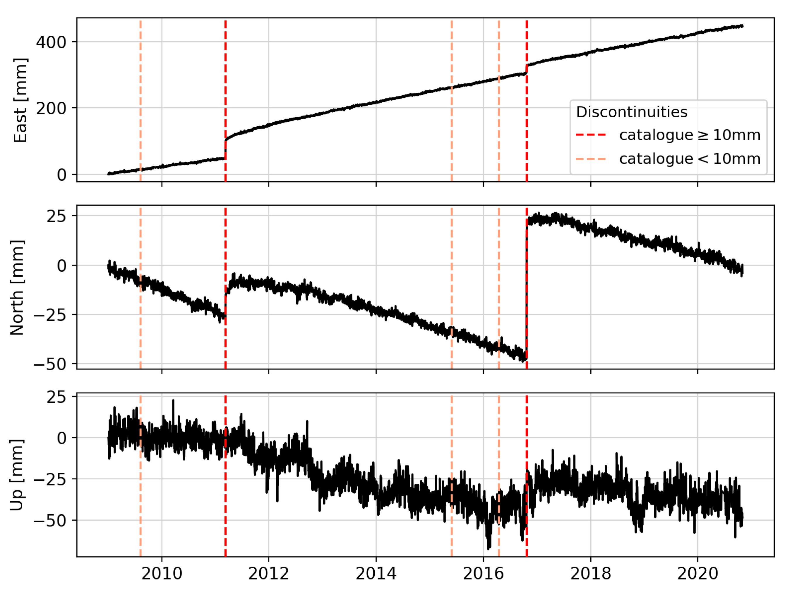
The GPS station coordinate time series are taken from the Nevada Geodetic Laboratory (NGL) [21]. NGL provides open access to geodetic GPS solutions from more than 19,000 stations around the globe. The solutions are updated daily and are available as simple text files. The processing strategy of the GPS data with all its details can be found on the NGL website (http://geodesy.unr.edu/ (accessed on 30 August 2021)). Besides estimated station positions, other products are available as well, such as troposphere products, velocity fields, and a database of potential discontinuities. For our analysis, we use the provided daily station coordinate time series as well as the database of the potential discontinuities. It is distinguished between two types of discontinuities: equipment changes taken from the International GNSS Service (IGS) log files (antenna, receiver or firmware change) and potential discontinuities caused by earthquakes. Figure 1 shows an example of the station coordinate time series of a GPS station. All potential discontinuities caused by earthquakes from the NGL discontinuity database are represented by vertical lines. The colour of the lines serves to differentiate between earthquakes that cause a displacement above and below a threshold of ten millimeters.
Earthquake discontinuities are listed if their epicenter is within a threshold distance d of the station. The threshold distance d is calculated using a simple formula based on the magnitude M of the earthquake:
The information about when an earthquake happened is provided by the United States Geological Survey (USGS). Further information like the USGS event ID, the threshold distance for the event, the distance from station to epicenter and the event magnitude can also be found in the database.
2.2. Study Region
In this study, Japan was selected as the test area. Its geographical location along the Pacific Ring of Fire makes it an earthquake-prone region. The whole country is in a very active seismic area and thus experiences a lot of earthquakes of different magnitudes. Since 1996, 239 severe earthquakes (https://www.kyoshin.bosai.go.jp/cgi-bin/kyoshin/bigeqs/index.cgi?E (accessed on30 August 2021)) have been recorded by two high-motion seismograph networks, K-NET (Kyoshin Network) and KiK-net (Kiban Kyoshin Network), that were established by the National Research Institute for Earth Science and Disaster Resilience (NIED).
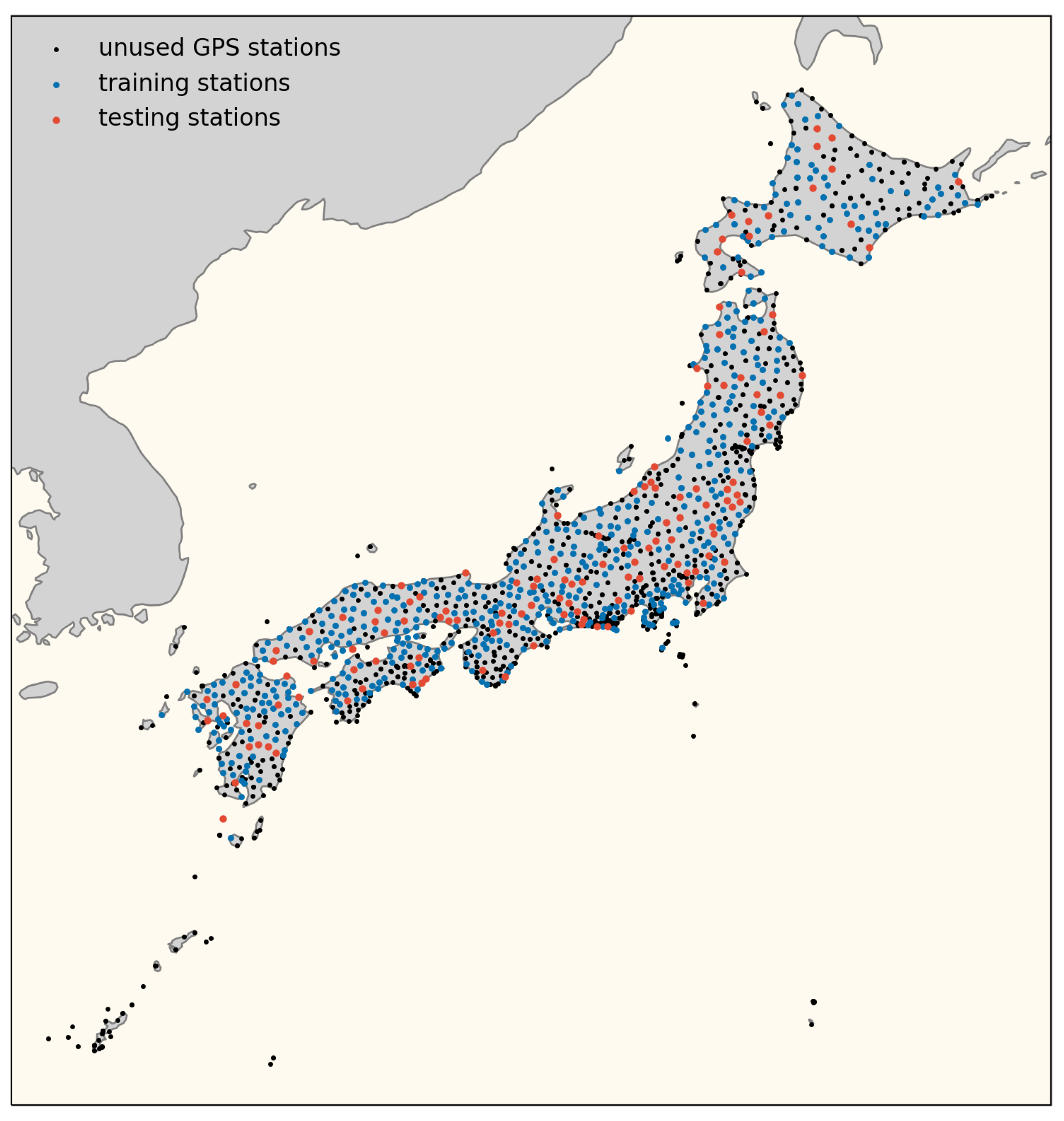
For our study, all GPS stations of Japan available on the NGL website are selected. At the time of acquisition, there have been 1449 stations available. From all these Japanese stations, a subset of suitable stations is selected based on two criteria. First, only stations recording a structural break caused by an earthquake that is equal to or larger than ten millimeters, are selected to make sure that significant displacements are present in the data. Second, only stations with less than 0.5% of missing values are selected. These criteria ensure that only stations are used that have at least one structural break that should be detected and very few missing values. It results in a total of 665 stations. Figure 2 in Section 3 depicts a map containing the station locations.
3. Methods
The aim of this study is to detect structural breaks caused by earthquakes in GPS station coordinate time series. To achieve this goal, a classification problem is formulated and solved using machine learning. It is classified whether an earthquake has happened within a certain time span, and therefore, a structural break has occurred within this time span or not. Since a database of potential discontinuities is available from the NGL, supervised machine learning algorithms are used.
The classification is carried out for the selected subset of suitable stations (described in Section 2). First, the data are randomly split into 80% training and 20% testing stations. This results in 532 training stations and 133 testing stations as depicted in Figure 2. A machine learning model is trained based on the coordinate time series of the training stations. The station coordinate time series are split into individual chunks as described in Section 3.1. Based on the NGL discontinuity database, chunks containing earthquakes are flagged. While fitting the model, a three fold cross-validation is carried out to tune the hyperparameters of the algorithm, see Section 4.2. Based on the fitted model, predictions of whether and when a structural break happened, are made and compared with the entries of the NGL discontinuity database for the training and testing stations. The predictions regarding the training stations are done to know if the fitted model is overfitting. Overfitting shows that the model is not generalising well and, therefore, is not able to perform well on unseen data [22]. The predictions of the testing stations serve to validate the model as they are not used to train the model. Thus, the performance of the testing stations is a measure of how well the model performs on unseen data.
As a primary step, the analysis is limited to earthquakes causing a significant station coordinate displacement since detecting these earthquakes is most important for potential applications. Therefore, only structural breaks causing a station coordinate displacement equal to or larger than ten millimeters are flagged, i.e., as an example, only the vertical dark red lines shown in Figure 1. Typically, this is sufficient for many applications, including a velocity estimation from GPS station coordinate time series as will be demonstrated in Section 4.10. The noise floor in the data is defined as the median of a rolling standard deviation over 30 days. It is 1.71 mm for the east, 1.59 mm for the north, and 5.19 mm for the up component. In Section 4.4, the impact of a threshold of ten millimeters as well as other values is further discussed. The displacement size itself is calculated based on the difference of the median of the time series seven days before and seven days after the reported structural break.
The classification is formulated as a multi-class classification problem where the time within the chunk when the structural break is reported represents the class label as further described in Section 3.2. The advantage of multi-class classification compared to binary classification is that additionally to the information of whether a discontinuity happened or not, the time of the discontinuity can be detected, which is important information. Furthermore, previous internal investigations concluded that multi-class classification works better. It achieves comparable recall but significantly better precision and F1 score than binary classification.
3.1. Structure of Feature Matrix
The features used in the machine learning algorithm are the GPS station coordinate time series of the selected stations. All stations provide three time series for the individual coordinate components, namely, east, north, and up. The time series are split into n chunks of m days.
The splitting is done in an overlapping manner, so that the first chunk contains day one until day m, while the second chunk contains day 2 until day . This means that a 365 day long time series with a chunk size of leads to chunks of 21 days.
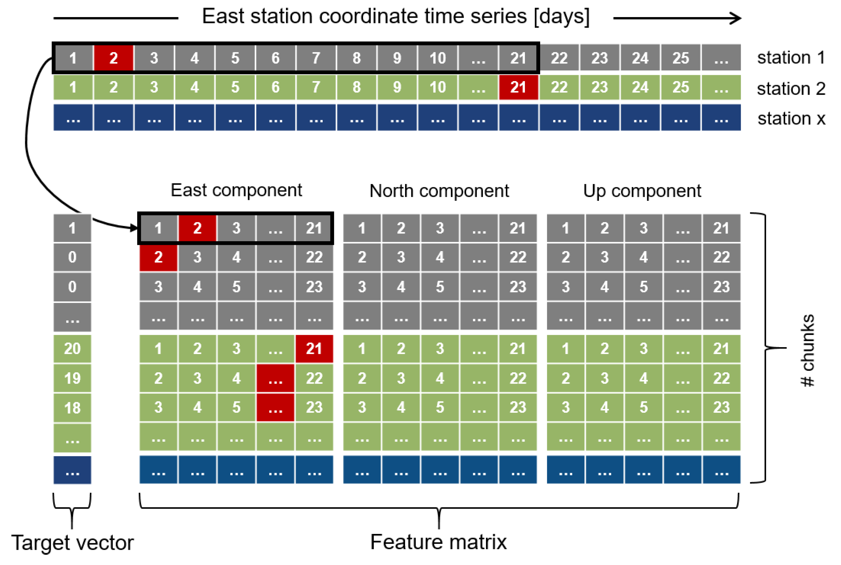
In Section 4.7, different feature matrix layouts are tested. For illustration purposes, one option that was investigated is depicted in Figure 3. It works by combining the individual chunks per component to one sample (row of the feature matrix, respectively). This constellation leads to features used in the machine learning model. Thus, the resulting feature matrix of one station has dimension . All stations are used together to form the feature matrix and to train one common model.
The used machine learning methods are not able to deal with missing values. Since there is enough training data available and missing data do not occur that frequently, chunks including missing values and outliers (see Section 3.4) are simply discarded to avoid inserting noise.
Additionally, all chunks are removed that contain a day of when an equipment change is recorded in the discontinuity database since the focus in this study is to train a model to classify structural breaks caused by earthquakes and not for equipment changes. Equipment change cause structural breaks in GPS time series that would distort the training of the machine learning classification. It is worth noting that the machine learning model suffers if discontinuities are missing in the database, i.e., inaccurate labeling. However, if the number of missing discontinuities is not very pronounced, the machine learning model should be robust enough and not be distorted.
3.2. Structure of Target Vector
The target vector contains the information of whether a structural break occurred in the corresponding chunk or not. Since multi-class classification is used, the target vector does not only contain binary information but represents the time at which a structural break is happening inside this chunk (starting at zero), or zero if no structural break occurs. It is worth noting that this method is not able to distinguish between no structural break inside the chunk (class 0) and a structural break happening on the first day of the chunk (also class 0). This is intentional and the reason for this is that if a break happens on the first day, then no information before the break is available. Thus, also visually, no break or jump in the time series would be detectable. The structure of the target vector is shown in Figure 3.
3.3. Validation
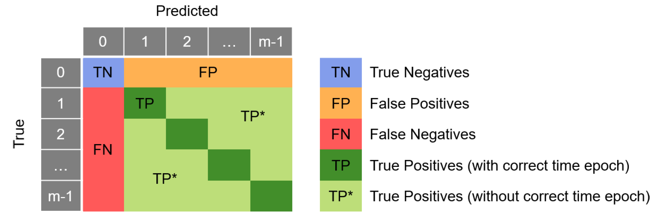
A common metric to validate a classification model is the confusion matrix. It evaluates the classification accuracy and reports the number of false negatives (FNs), false positives (FPs), true negatives (TNs), and true positives (TPs). The TPs indicate how many structural breaks are correctly classified as structural breaks, whereas the TNs indicate how many chunks containing no structural breaks are correctly classified as having no structural breaks. The errors done by the classification are indicated by FNs and FPs. The FNs indicate structural breaks that are wrongly classified as no structural breaks, whereas the FPs indicate chunks without a structural break which are still classified as having a structural break. For our analysis, the FNs are the most critical errors, since we do not want to miss any structural break.
Out of the confusion matrix common performance measures that can be calculated, like precision, recall, and F1 score.
The precision indicates the percentage of true structural breaks among all structural breaks detected by the machine learning algorithm. The recall shows the percentage of correctly detected structural breaks among all existing structural breaks. Typically, recall and precision have an inverse relationship. The F1 score is the harmonic mean between precision and recall. It ranges between 0 and 1, with 0 being the worst score, indicating precision or recall to be zero and 1 being the best score, indicating perfect precision and recall. In the case of multi-class classification, the confusion matrix is expanded for each individual class, therefore, leading to the dimension of , as illustrated in Figure 4. Thereby, class 0 represents no structural break happening, while the other classes represent cases where a structural break happens (see Section 3.2). Thus, the classes can be grouped into two overall classes, 0 for no structural break and 1 to for classes with structural breaks. Therefore, we do not look at the FNs, FPs, TNs, TPs of each individual class, but we summarise the predictions made for class 1 to and calculate the precision, recall, and F1 score based on these summarized measures. Additionally, we extract the information of whether the time of the structural break is detected correctly. Thus, we have two types of true positives: TP that are representing correctly classified samples where, additionally, the time of the discontinuities is correctly classified and TP* that are representing correctly classified samples but the time of the earthquake is incorrectly classified.
Another often used measure for classification is the receiver operating characteristic (ROC) curve [23]. It plots the true positive rate (TPR) against the false positive rate (FPR) at various discrimination thresholds. The TPR is another term for recall or sensitivity, whereas the FPR is also known as fall-out and indicates the percentage of falsely detected structural breaks among all non-existing structural breaks.
When plotting the ROC curve, the so-called area under the curve (AUC) can be computed as its integral, which summarizes the curve characteristics in one number. The highest possible AUC is one, while the lowest possible value is zero. The higher the number, the better the classifier. Random classification leads to an AUC of 0.5.
3.4. Pre-Processing of Training Data
To train the classification model, the time series used for training are pre-processed. This is necessary to have a good quality of the time series to train a good model. In particular, one of the main challenges is the highly imbalanced class distribution with a majority of class 0 (chunks with no earthquake), see Section 4.8. Therefore, it is necessary to get a clean representation of this class without loosing information about the other classes.
The pre-processing of the training data is divided into several parts. First, an outlier detection is applied; then, an exclusion of noisy areas within the time series is done.
To detect outliers, first the noise floor of the time series is determined. This is done by taking the median of a rolling standard deviation of the time series. Then, a rolling median of the time series is subtracted from the original time series. All data points are excluded where the absolute difference is bigger than five times the noise floor. Using a value of five times the noise floor for the outlier detection was selected based on empirical tests. In many geodetic applications, an outlier threshold of three times the standard deviation is used. Here, it was found that using a value of three leads to more false-positive outlier removals. Thus, for the sake of this application, using five times the standard deviation works better.
The exclusion of noisy areas within the time series is done in a similar way. It is applied to the time series where the outliers are already removed. First, again, the median of the rolling standard deviation of the time series is taken as a measure for the noise floor. Then all data points are excluded, where the rolling standard deviation is bigger than two times the noise floor. Again, the threshold of two times the noise floor is defined empirically.
However, in both of these steps, it is ensured that the m days before and after a structural break are never removed from the time series. This is done because otherwise, earthquakes or post-seismic deformation will simply be labeled as outliers or noisy areas and thus removed from the time series. However, this should not happen, since in particular the data before and after an earthquake is needed in order to be able to detect it.
For reference, after these data pre-processing procedures with , about 84% of the data remains. These pre-processed time series are then used to build the feature matrix as described in Section 3.1.
Finally, two more processing steps are necessary. First, all chunks containing earthquakes causing a structural break smaller than ten millimeters are removed from the training data. This is, again, done to get a clearer representation for class 0 with respect to the highly imbalanced dataset. Tests revealed, that it is better, that these small jumps, that are below our selection criteria, are not part of the training for class 0 to not confuse the machine learning algorithm. Second, all chunks up to 14 days after the earthquake are removed. This is done because the time series after an earthquake is oftentimes not very stable due to post-seismic deformation or aftershocks. Tests did reveal that this could disturb the training of the machine learning model and, therefore, it is better to remove these chunks during training.
It is worth noting that all the pre-processing steps are only done for the training data and not for the testing data because these steps partly rely on the information of whether an earthquake happened or not, which in turn, should be detected by the machine learning algorithm itself. The idea of the pre-processing is to get a clearer representation of the individual classes during training. Thus, for applying the derived machine learning model on new datasets, no pre-processing is necessary.
4. Results
To exploit the full potential of the machine learning algorithms and to make the algorithm learn whether a structural break occurred or not, several considerations and a lot of experiments have been performed, among which the most important findings are presented in this section.
To give the reader an overview about our findings while keeping the number of investigations and results small, the tests are grouped into different topics or tasks, e.g., finding a proper chunk size, testing different feature setups, or investigating different model designs. Each topic is presented in one subsection.
It is worth noting that the results of the individual experiments that are presented in the following subsections cannot be viewed independently. Instead, they all interact with each other and it is necessary that their investigation is carried out simultaneously and iteratively. Thus, some of the presented investigations are already making use of findings based on results from previous investigations that will be discussed in a later subsection.
4.1. Different Machine Learning Algorithms
As a very first step, ten different machine learning algorithms are tested to find out which one might work well for our study. The tested algorithms are:
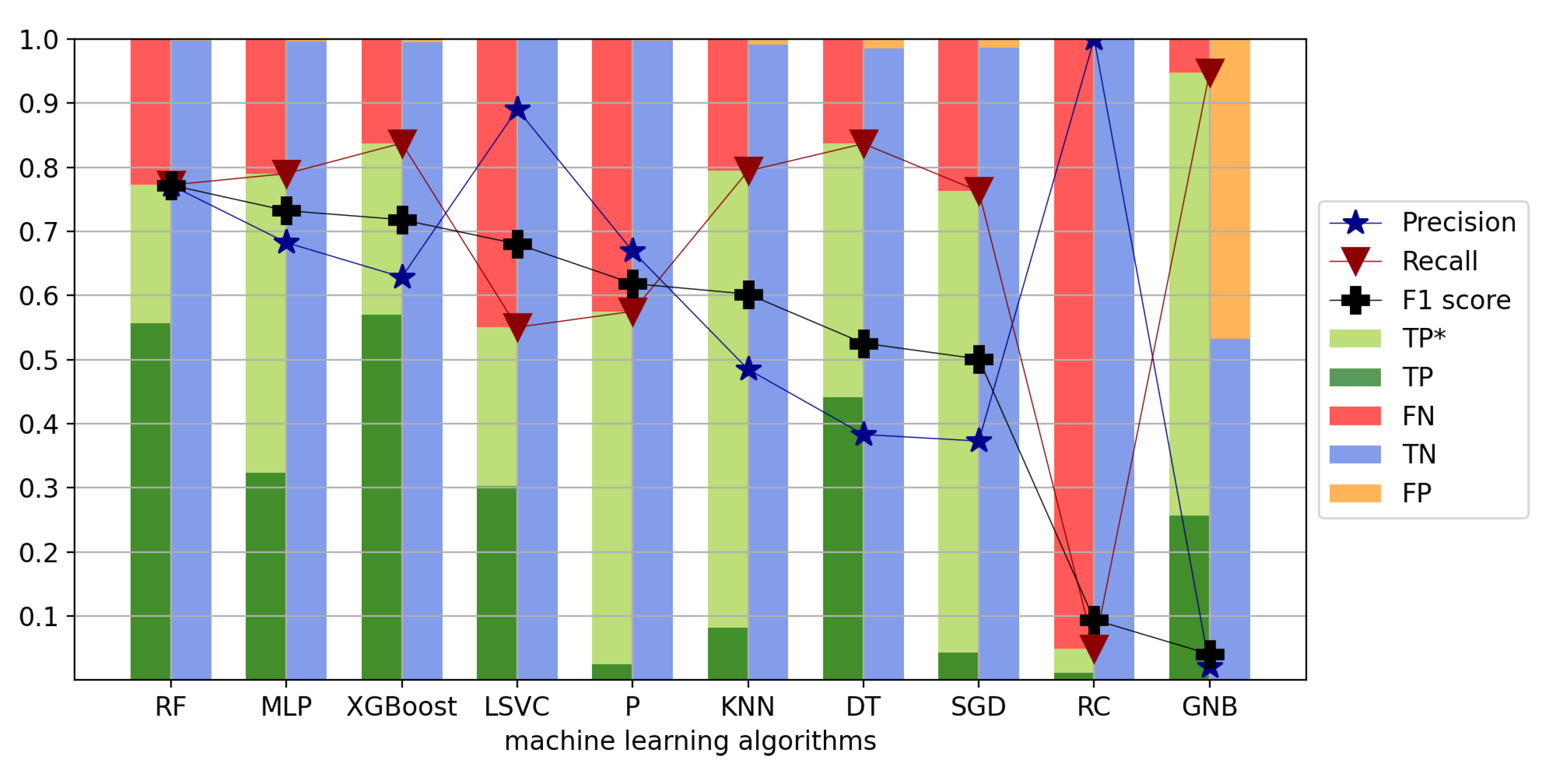
For this investigation, the feature selection, the model constellation, and the chunk size have been used as discussed in the upcoming Section 4.5, Section 4.6 and Section 4.7. The results are summarized in Figure 5.
Random Forest stands out because it has the highest F1 score (0.77) and its precision and recall are equally high. Additionally, MLP and XGBoost also work reasonably well. The F1 scores are a bit lower compared to Random Forest (0.73 for MLP and 0.72 for XGBoost) as well as the precision; however, the recall is slightly higher. The algorithms LSVC and P perform a bit worse with an F1 score of 0.68 and 0.62, respectively. For these two algorithms, the precision is higher than the recall. The F1 score drops further for KNN (0.60), DT (0.53), and SGD (0.50), and the precision and recall diverge even more. These methods achieve a higher recall at the cost of lower precision. The methods that did not work at all are RC and GNB. RC, which is a linear classification algorithm, has a recall of only 0.05 and an F1 score of 0.09. GNB achieves a high recall of 0.95, at the cost of a very low precision of 0.02, leading to an F1 score of 0.04.
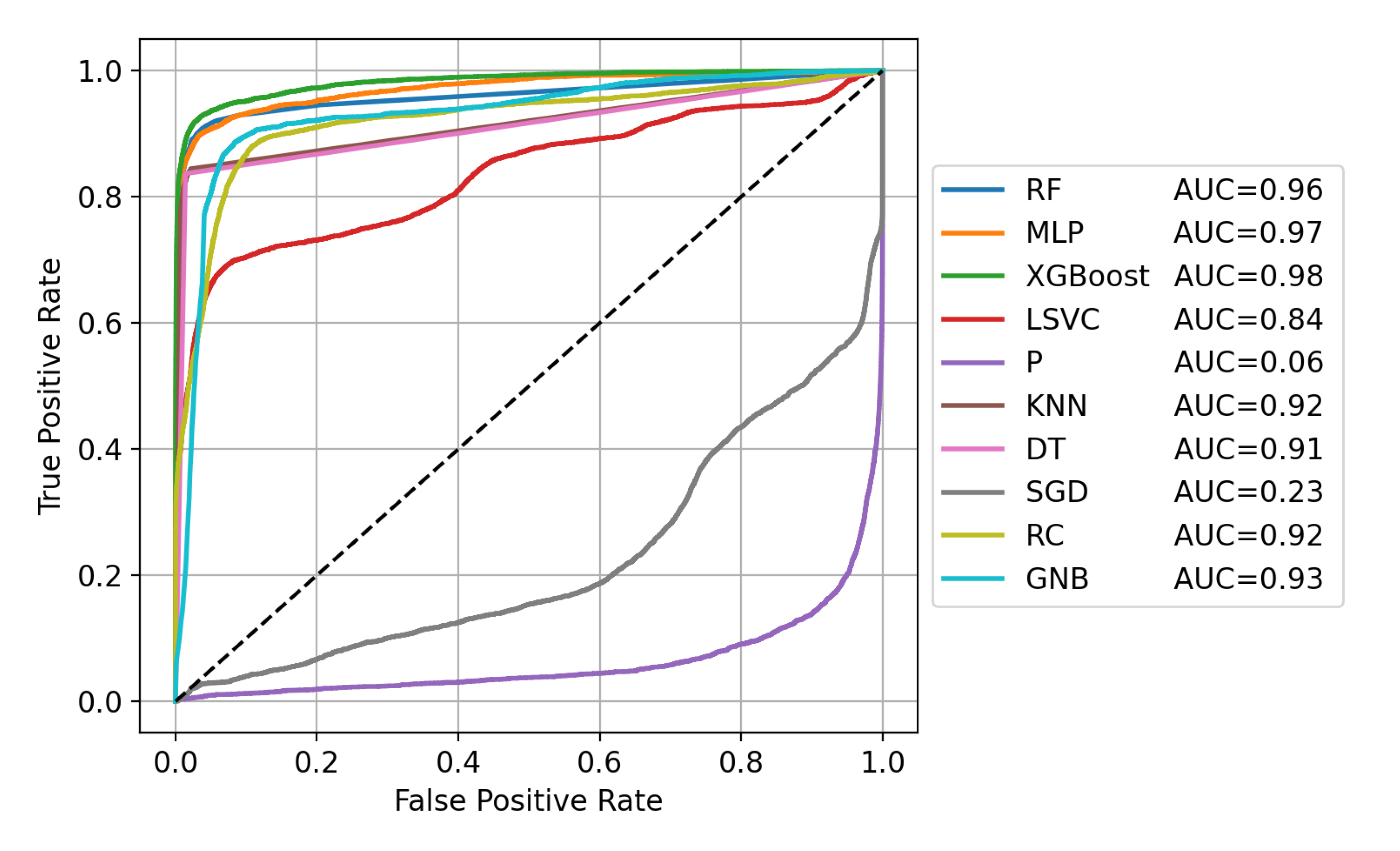
Additionally to the results shown in Figure 5, the ROC curve and the AUC for the different machine learning algorithms are depicted in Figure 6. Using these performance metrics, it can be seen that three methods reach high AUC values, namely, XGBoost (0.98), MLP (0.97) and RF (0.96). Interestingly, RC and GNB, which show the poorest performance in regards to F1 score, achieve a very high AUC of 0.92 and 0.93, respectively. On the contrary, the lowest AUC have SGD (0.23) and P (0.06), which both have a moderate F1 score.
In summary, three methods provide high F1 scores while having a high AUC, namely, RF, MLP, and XGBoost. Although XGBoost has the best recall, it also has the lowest precision. MLP has a problem of correctly classifying the correct earthquake epoch within a chunk, as can be seen based on its low number of TPs compared to TPs*. Therefore, RF is selected as the primary method for further analysis. It achieves the highest F1 score while also providing the best compromise between precision and recall. Furthermore, its ratio between TPs compared to TPs* is also very high, indicating that the correct epoch of earthquakes can also be derived very well.
4.2. Hyperparameter Tuning
After identifying Random Forest as a suitable algorithm for our purposes (see Section 4.1), a more extensive hyperparameter optimization is carried out. The purpose of the hyperparameter tuning is to determine optimal properties of the models to gain highest performance. Examples for hyperparameters for Random Forest are the number of trees that should be trained, the maximum depth of the trees, the minimum number of samples required to be at a leaf node, and the minimum number of samples required to split a node.
To choose ideal hyperparameter values, a grid search is conducted, which is an exhaustive search over a subset of manually selected values. The performance of all hyperparameter value combinations is evaluated based on a three-fold cross-validation. This means that only two thirds of the training data are used for training directly, while one third is used for validation. This is repeated three times until every sample is once picked for validation purposes. The average performances of the validation sets of these three runs per hyperparameter value combination are compared to identify the best set of hyperparameter values. The tested hyperparameter values, as well as the best performing hyperparameter value combination, are summarized in Table 1. In total, hyperparameter value combinations are investigated.
After the hyperparameter tuning the F1 score stays 0.77. The recall increased from 0.77 to 0.78 while the precision changed from 0.77 to 0.76. Thus, it can be concluded that the hyperparameter tuning did not significantly improve the prediction performance and the default parameters also worked reasonable well in our case.
4.3. Error Analysis
The confusion matrix (see Figure 4) reports the errors obtained by the classification algorithm. These errors are further analysed in this section.
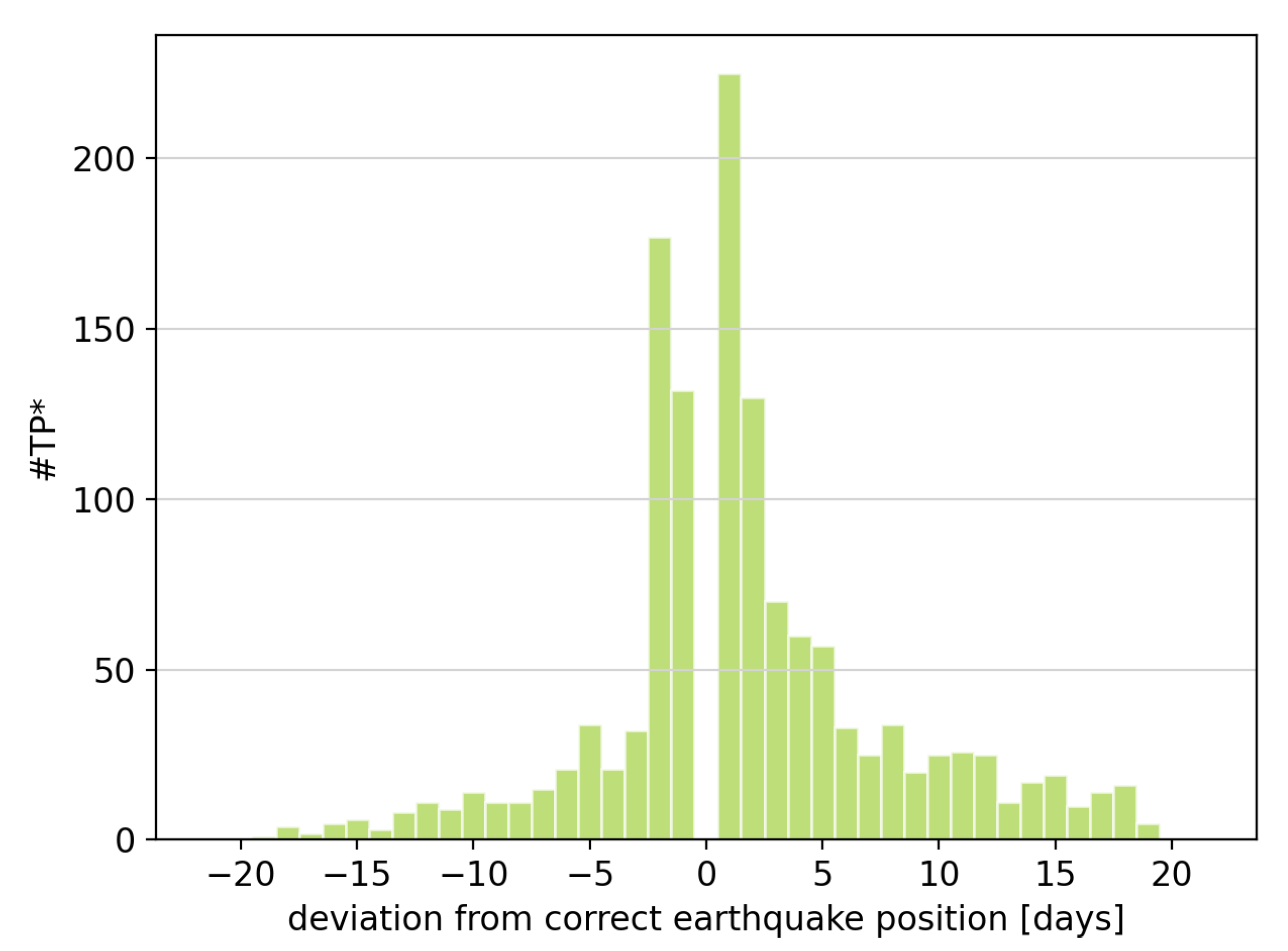
In total, there are 5613 samples among the testing data containing an earthquake. In 22% of the cases, the earthquake could not be detected (FN) and in 78% of the cases, the occurrence of an earthquake was correctly classified (TP+TP*). Additionally, in 54% of all cases, the epoch of the earthquake was correctly classified as well (TP) while it was not possible for the remaining 24% of the cases (TP*). In most of these cases, the deviation between the true and classified earthquake time is only one to two days with a root mean squared error of 3.7 days. Figure 7 depicts a histogram of the error in time of classified earthquakes.
Furthermore, there are 537,499 samples among the testing data containing no discontinuity caused by an earthquake. In 99.7%, it was possible to correctly classify those samples (TN), whereas only 0.03% of the samples were wrongly classified (FP).
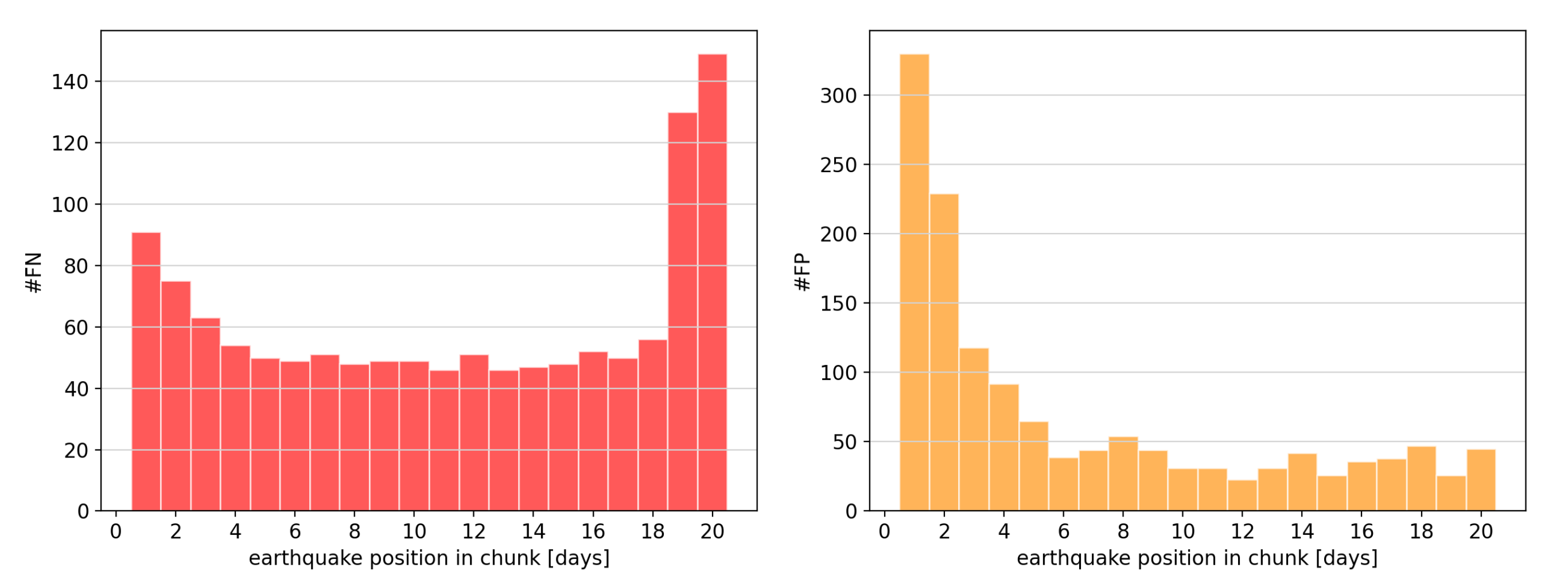
Figure 8 shows how the FNs and FPs are distributed regarding the earthquake position within the chunk using a chunk size of 21. The FNs mostly occur if the earthquake is located at the beginning or at the end of the chunks. This is reasonable since for displacements happening at the beginning or at the end of the chunk there is fewer data showing the displacement.
The FPs seem to occur mostly at the beginning of the chunk, meaning that if the machine learning algorithm wrongly detects an earthquake, it is most of the time located at the beginning of the chunk. Surprisingly, there are not significantly more FPs for earthquakes reported at the end of the chunk.
So far, the presented results have always been focusing on the performance based on the provided samples. Due to the nature of the presented algorithm, an actual earthquake will show up in up to m samples with m being the chunk size. In case the result is viewed based on actual earthquakes instead of samples, the NGL discontinuity database includes a total of 565 earthquakes causing a displacement equal to or larger than ten millimeters for the 133 investigated testing station. Random Forest was able to correctly classify 524 of these earthquakes. In 438 cases, the time of the earthquake was correct as well (TP), while in 86 cases, the exact time of the earthquake could not be classified (TP*). The remaining 41 earthquakes could not be detected by the machine learning algorithm (FN).
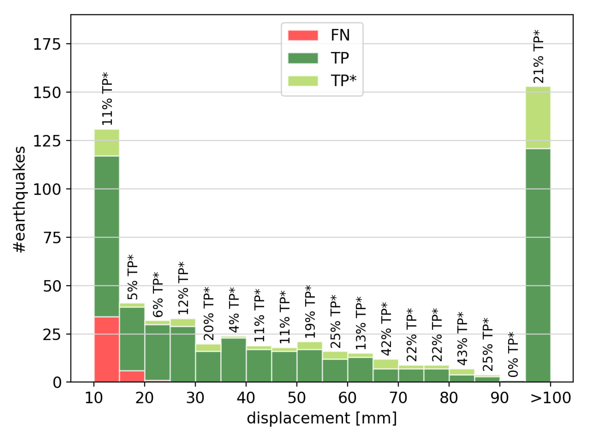
Furthermore, we have investigated whether there is a pattern between the classification accuracy and the earthquake displacement size. Figure 9 depicts histograms of the FNs, TPs and TPs* in relation to the earthquake displacement size. The sum of FNs, TPs and TPs* corresponds to the total number of earthquakes. It is worth noting that earthquakes causing a displacement larger than ten centimeters are combined in the last bin.
Almost all FNs occur for earthquakes causing a displacement smaller than 20 mm. This means that earthquakes causing a bigger displacement are always detected correctly, which can be seen when looking at the TP + TP* in the histogram. The number above each bin displays the percentage of TPs* of all earthquakes in this bin. On average there are 17% TPs* in each bin. For bigger earthquakes causing a displacement larger than five centimeters, the number of TPs* tends to increase, which means that the method has troubles to correctly classify the time for the earthquake. This might be explained by the more infrequent occurrence of these earthquakes leading to less training data or also the non-linear post-seismic deformation or gaps in the data of big earthquakes.
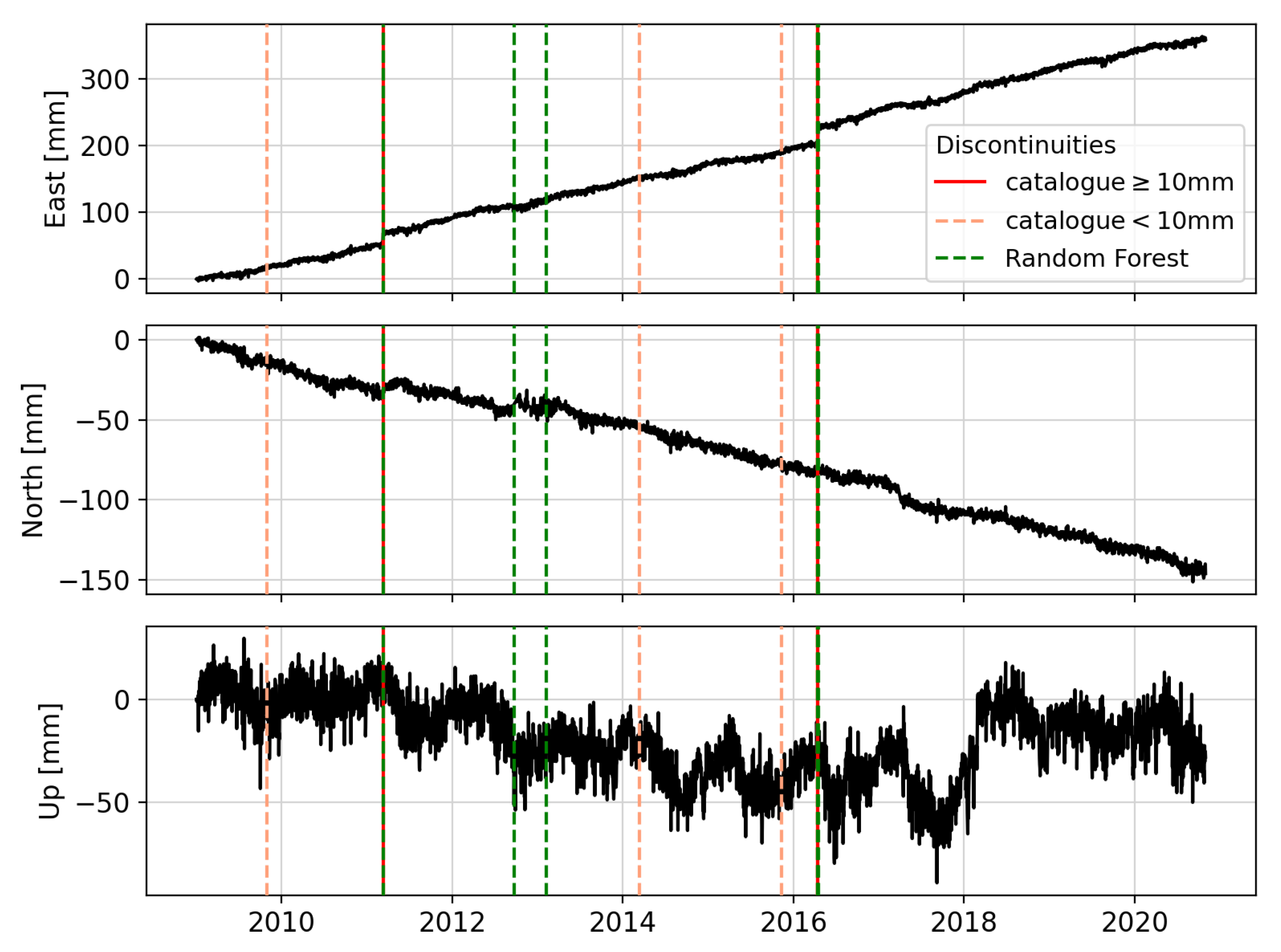
Figure 10 serves to give the reader an impression of how the result of the machine learning algorithm looks like for a single GPS station. For this station, Random Forest detects in total four discontinuities. Two detected discontinuities are TPs, while the other two detected discontinuities are FPs, since the catalogue does not list them. However, it seems, especially when looking at the first FP, that a discontinuity is still in the Up and North component of the time series. Thus, it might be that Random Forest is correct and the discontinuity is missing in the catalogue.
4.4. Different Thresholds for Displacement Size
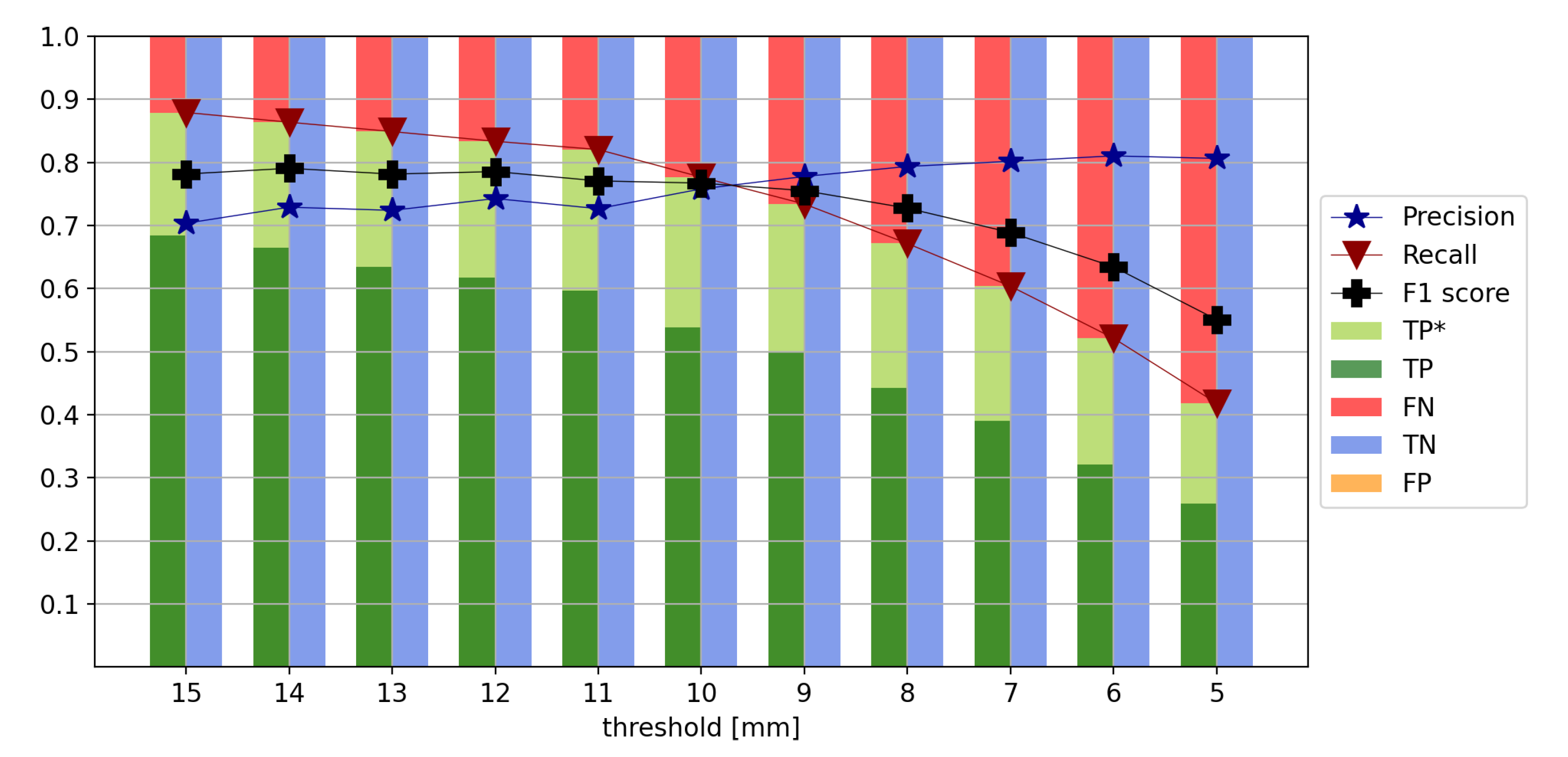
As already mentioned in Section 3, the machine learning algorithm is trained to only detect structural breaks causing a station coordinate displacement equal to or larger than ten millimeters. This threshold needs to be chosen to build a well performing model. To decide which threshold is appropriate, different thresholds between 5 and 15 mm have been tested. Figure 11 summarizes the results. In general, it can be concluded that the lower the threshold, the lower the performance. This makes sense since smaller displacements are more difficult to detect. When looking at the F1 score, it can be seen that it is almost constant for thresholds between nine and fifteen millimeters. However, when using thresholds from five to eight millimeters it is significantly lower. The result when using a threshold of ten millimeters shows equally high recall and precision. All results using a threshold bigger than ten millimeters have a higher recall than precision, whereas all results using a threshold smaller than ten millimeters have a higher precision than recall.
Due to this analysis, a threshold of ten millimeters is found to be optimal since a high F1 score is achieved and, at the same time, a threshold of ten millimeters is more sensitive to smaller earthquakes than larger thresholds.
4.5. Feature Selection
As discussed in Section 3.1, chunks of GPS station coordinate time series are used as features to classify whether and where a structural break happened. Therefore, different features are generated and tested to try to improve the performance of the classifier. Several options for features exist:
- use chunks of pre-processed data directly (O)
- normalize the chunks (N)
- add the value range as additional feature (R)
- combine individual components into 3D displacement and add it as additional component (3D)
- add first derivative as additional feature (FD)
- add second derivative as additional feature (SD)
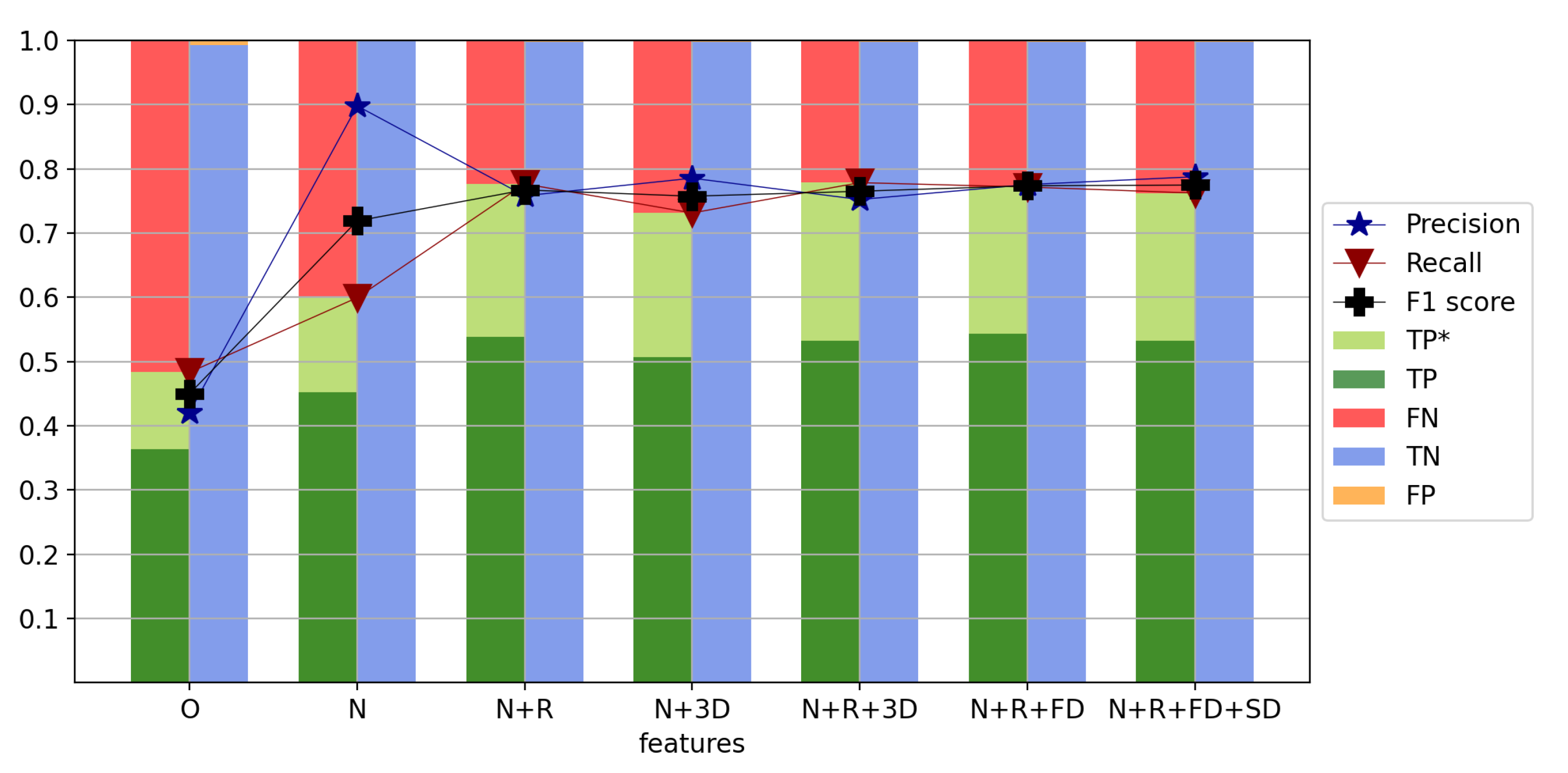
The results of the different investigations can be found in Figure 12.
In a first test, it is investigated if a normalization of the individual chunks helps to gain a better performing model. A normalization is typically conducted for numerical reasons [38,39]. By comparing the performance with and without normalization, it can be seen that the F1 score improves from 0.45 to 0.72 by normalizing the chunks. This significant performance increase leads to the conclusion, that a normalization of the chunks is beneficial.
Next, it is investigated if the inclusion of additional features increases the performance of the model. Since the main task in this study is to identify structural breaks featured as jumps in the time series, one obvious feature to add is the value range within each chunk, which is defined as the maximum value minus the minimum value before normalization. The idea is that the value range of chunks with a structural break is significantly larger compared to the value range of chunks without a structural break since in cases without structural breaks, it is only mainly driven by measurement noise, while in cases with a structural break, the resulting jump in the coordinate value is depicted as well. Using the ranges leads to a slight drop in the precision; however, the recall improves significantly leading to an improvement of the F1 score from 0.72 to 0.77.
A similar effect is achieved by including the 3D displacement of the chunks instead of the ranges. To compute the 3D displacement, the square root of the squared sum of the east, north and up components is taken as a new, fourth component. By adding this new component into the feature matrix, the F1 score can be improved from 0.72 to 0.76. Adding both, the value range and the 3D displacements simultaneously does not improve the F1 score any further, it stays at 0.77. Therefore, it is concluded that it is best to only include the value range as an additional feature.
Another idea is to include the first and second derivatives of the chunks. In the case of the first derivative, additional new features are added, while for the second derivative, new features are added. However, adding these new features does not lead to any improvements as can be seen in Figure 12.
In summary, it can be said that a normalization of the chunks is beneficial, and either the range of the values should be added as an additional feature per chunk, or the 3D displacements should be added as a fourth component. Using both, the range and the 3D displacement together did not improve the result. Neither did the addition of the first and or second derivative.
Within the other sections of this study, the presented results are all calculated based on normalized chunks and by adding the range as an additional feature.
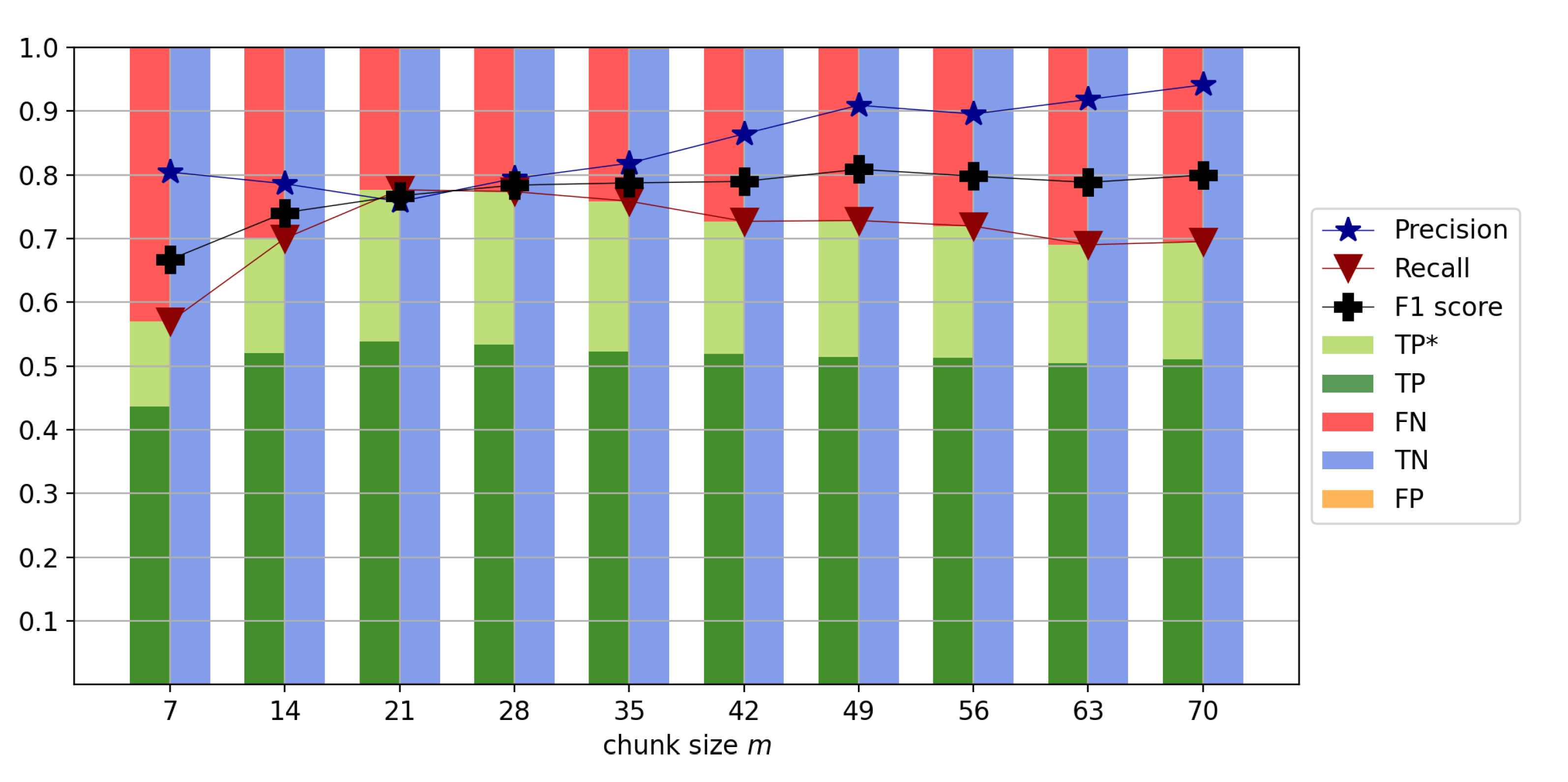
4.6. Impact of Chunk Size
To choose the optimal chunk size, chunk sizes between seven and seventy days are tested. The classification results are shown in Figure 13. It can be seen that the F1 score increases until using a chunk size of 28 days and remains relatively flat thereafter. The recall, in turn, increases until using a chunk size of 21 days and decreases again from a chunk size of 28 days. However, from using 35 days onwards, the gap between precision and recall becomes larger and larger. Thus, either 21 days or 28 days are good candidates for appropriate chunk sizes. The performance of the two is very similar, with an F1 score of 0.77 for a 21 day chunk size and 0.78 for a 28 day chunk size. For the remaining part of this study, a chunk size of 21 days is used for the following reasons: First, the recall is slightly higher with 0.78 for 21 days compared to 0.77 for 28 days. Next, a smaller chunk size leads to fewer chunks with multiple earthquakes—something that is not properly accounted for in this work and will be further investigated in upcoming studies. Applying a chunk size of 21 yields to a total of 1,863,250 chunks from the 532 training stations and 543,112 chunks from the 133 testing stations.
4.7. Different Model Constellations
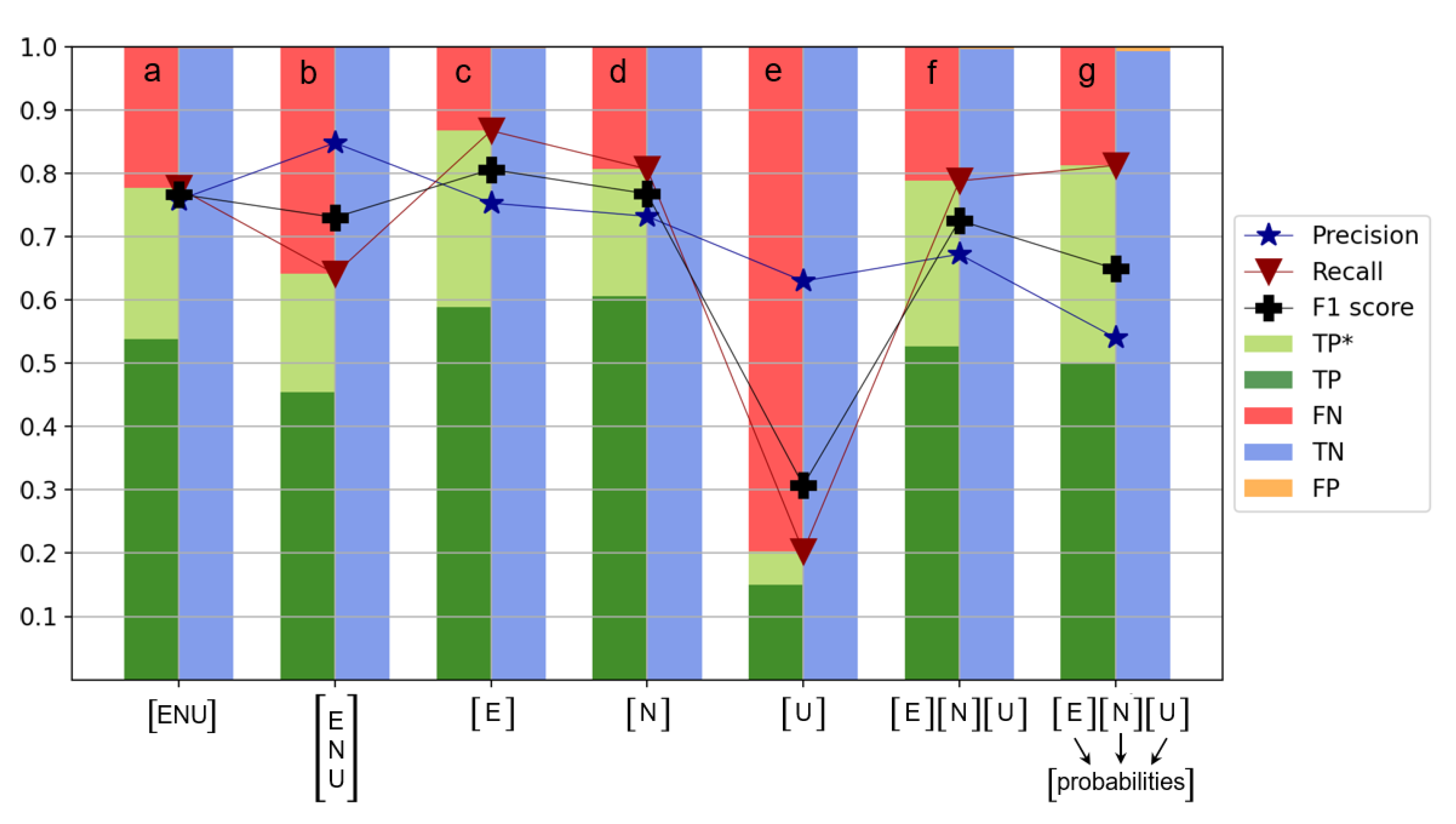
In Section 3.1, we already visualized how the structure of the feature matrix looks like if the chunks from the individual components (east, north, up) of one station are combined into one sample. As already shown in the last sections, the resulting performance based on this approach is 0.77 for the F1 score. For comparison reasons it is again visualized in Figure 14a. However, other options exist and are worth being investigated.
One alternative is the straightforward approach of assigning every chunk from each individual component to one sample. Therefore, one would get three times more samples with only one third of the features. However, this constellation does not lead to an overall improvement as can be seen in Figure 14b. Although the precision gets higher, the recall and F1 score are lower.
Another alternative constellation is to train one model for each individual component and then combine the results. The individual models for the east (Figure 14c) and North component (Figure 14d) perform well, whereas the model for the Up component (Figure 14e) achieves only low performance, as expected, since earthquakes are mainly causing horizontal and not vertical motions. For the final prediction of whether an earthquake happened at a station, one way is to simply look if any of the predictions from the individual component-wise models classified an earthquake, equivalent to a logical “or” operation (Figure 14f). This approach works well achieving an F1 score of 0.73; however, combining all components into one sample still outperforms it.
A last investigated alternative is to calculate the class probabilities from each individual model and train a second layer of machine learning model based on these probabilities, to derive the final prediction result (Figure 14g). However, this nested machine learning approach does not lead to a better classification performance and is only providing an F1 score of 0.65.
Within the other sections of this study, the presented results are all calculated based on combining the chunks of the individual components (east, north, up) of one station to one sample as already visualized in Figure 3.
4.8. Dealing with an Imbalanced Dataset
One of the difficulties in detecting discontinuities caused by earthquakes from chunks of GPS coordinate time series is the imbalance in the data. Most of the time (luckily) no earthquake happens and thus the majority of the chunks do not contain any discontinuities. Therefore, the classes are not represented equally, which poses a challenge to build a well working model. The imbalance can lead to poor predictive performance, specifically for the minority classes [40,41]. In our case, the minority classes are the discontinuities caused by earthquakes. The training data contains approximately 87 times more chunks without discontinuity than chunks with discontinuity given a chunk size of 21 days.
There are several commonly used approaches for dealing with imbalanced datasets such as oversampling the minority class or undersampling the majority class [42,43]. Additionally, for Random Forest, it is possible to assign class weights with respect to the class occurrence.
First, the class weights are adjusted inversely proportional to the class frequency in the input data. However, this did not lead to an improvement, the F1 score decreases from 0.77 to 0.68. As discussed in Section 3.3, there are two main groups of classes. One without discontinuities (class 0) and one with discontinuities (classes 1 – m), thus it was tested if class weights that are inversely proportional to the class group frequency would yield better results. However, the F1 score still did slightly decrease, from 0.77 to 0.76.
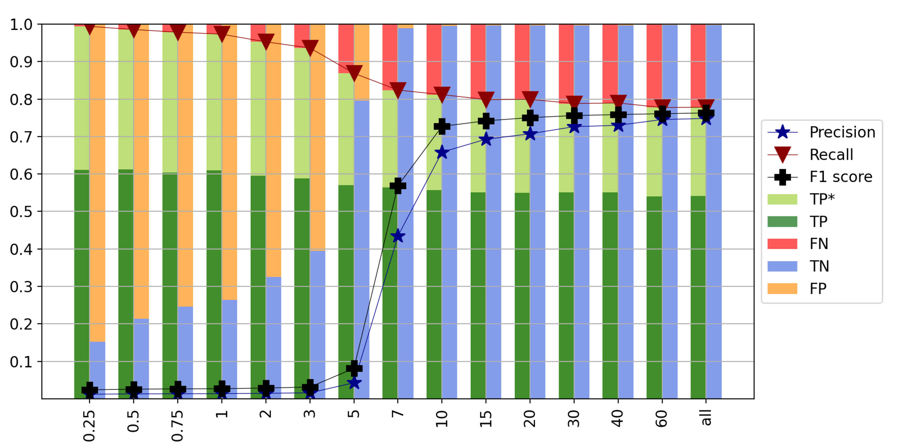
Next, it is investigated if random undersampling of the majority class helps in improving the prediction performance. This means that chunks containing no discontinuity are deleted randomly. In this way, the majority class is reduced and the class distribution is changed.
The amount of chunks that are removed is varied to understand its effect on the classification performance. The tested ratios between chunks with and without discontinuities ranges from 87 times more chunks without discontinuity than with discontinuity (full dataset) up to four times more chunks with discontinuities than without discontinuities. Figure 15 summarizes the classification results. While the recall is extremely high when having more chunks with than without discontinuities, the precision and thus the F1 score are extremely low. The higher the ratio gets, the lower the recall becomes. In contrast, the precision significantly increases with higher ratios, especially after a ratio of five. Therefore, the F1 score increases with a higher ratio.
Thus, based on this investigation, it was concluded that both approaches of accounting for the imbalance of the dataset did not yield an improvement in the performance. The best results could be achieved by simply using all the available data. Therefore, within the other sections of this study, the presented results are all calculated without special treatment of the imbalanced dataset.
4.9. Apply Model to All Available Japanese Stations
In Section 2, the selection of suitable stations for our study is presented. Based on two criteria, 665 of 1449 stations are selected. As discussed, the classification model is trained on 80% of the 665 stations and tested on the remaining 20% of the stations.
To investigate how well the trained model performs on all available Japanese stations, the same model is applied to all stations except the 532 training stations. The classification result shows only a slightly decreased performance. The recall, as well as the precision decrease, leading to an F1 score of 0.68 compared to an F1 score of 0.77 that was achieved for the selected suitable stations. The precision changed from 0.76 when using the selected suitable stations to 0.65 and the recall changed from 0.78 to 0.72. Therefore, one can conclude that the model is also able to make reasonable predictions for stations with lower data quality.
4.10. Validation Based on Uncertainties of Velocities Estimation
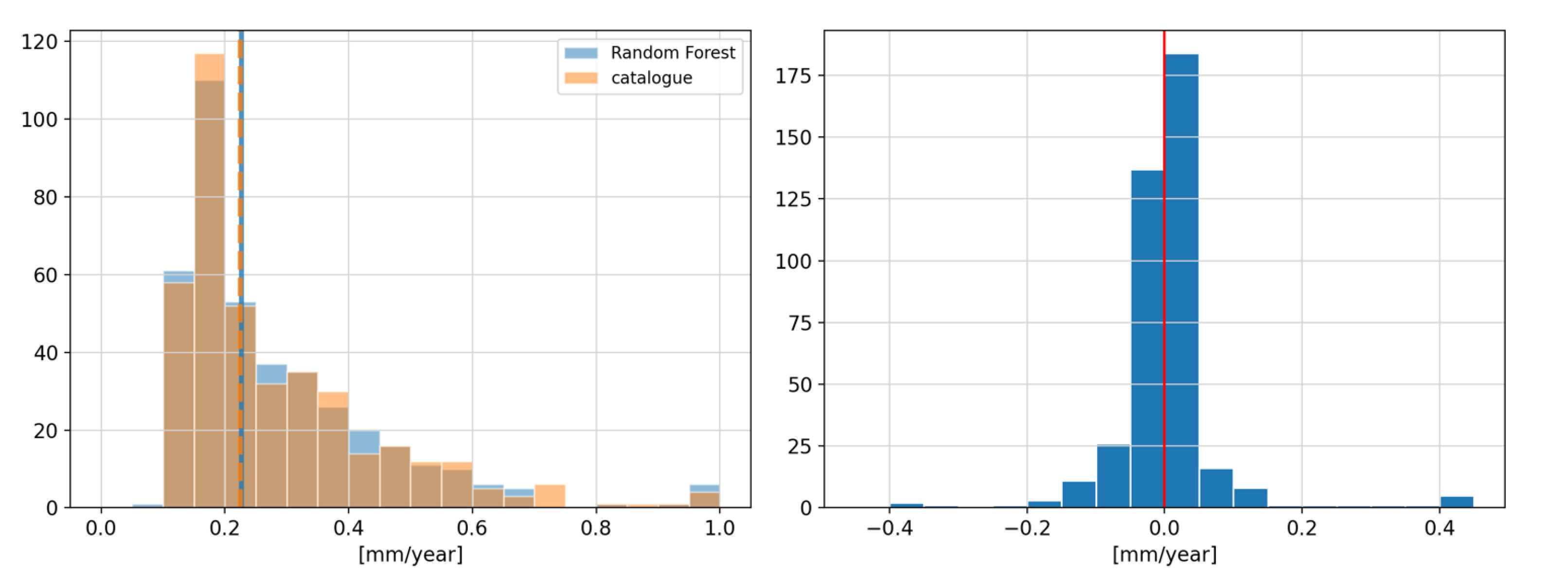
For an accurate station velocity estimation from GPS coordinate time series, a robust and discontinuity-free time series is necessary. One practical application to verify the quality of our machine learning based discontinuity classification is to compare the estimated station velocity uncertainties using the discontinuity information provided by our method with the estimated station velocity uncertainties based on alternative discontinuity information. For comparison, the discontinuities provided in the NGL discontinuity database, described in Section 2.1, are used. To calculate velocities and their uncertainties, the software package Hector [44] is used to properly account for seasonal and sub-seasonal signals within the time series. Figure 16 depicts the estimated velocity uncertainty based on both datasets.
In the left plot, the absolute values of the estimated velocity uncertainty are visualized. In blue, the result is calculated by using the discontinuities based on the proposed method while in orange, the result is calculated based on the NGL database. It can be seen that the two histograms match well, indicating that the performance of both approaches is equal. Furthermore, the median value is highlighted as a vertical blue line for the machine learning result while it is displayed as a vertical dashed orange line for the NGL database result. Both median values are nearly identical.
In the right plot of Figure 16, the difference between the estimated velocity uncertainty of each station component is visualized. It can also be seen that the majority of the differences are relatively small and below 0.1 mm per year. Values to the left of the red line (negative values) represent a better velocity uncertainty of the machine learning approach compared to the NGL database.
Thus, it can be concluded that the machine learning based discontinuity classification manages to work on a similar performance than discontinuity databases for the application of station velocity estimation without the need for external information.
5. Conclusions
In this study, it is demonstrated that it is possible to use machine learning algorithms to detect discontinuities in GPS time series that are caused by earthquakes by formulating the problem as a supervised classification task. Therefore, the GPS coordinate time series are split into individual chunks that are labeled and then fed into the machine learning algorithm.
Japan was chosen as a study area because of the high amount of GPS stations located there and due to the occurrence of many earthquakes.
It is demonstrated that the best result could be achieved by using a Random Forest classifier (see Section 4.1) with a chunk size of 21 days (see Section 4.6). The best performance is achieved by normalizing the chunks and by adding the value range as an additional feature (see Section 4.5). A combination of the chunks from the individual coordinate components to one common sample further improved the results (see Section 4.7). No improvement could be seen by trying to account for the imbalanced class representation (see Section 4.8).
Our final model was trained based on 1,863,250 and tested based on 543,112 samples. With our final model, the overall performance w.r.t the testing data can be expressed through an F1 score of 0.77 with a recall of 0.78 and a precision of 0.76. This means that among the testing samples, 4359 of 5613 (78%) can be correctly classified to contain a discontinuity caused by an earthquake (TP + TP*). Additionally, in 3020 (54%) of these cases, the time of the earthquake is correctly classified as well (TP), while it is not possible for the remaining 1339 (24%) of the cases (TP*). However, most of the time, the deviation of the correct earthquake position is only one to two days with a root mean squared error of 3.7 days. Furthermore, 536,108 of 537,499 (99.7%) of the testing samples could be correctly classified containing no discontinuity caused by an earthquake (TN). The number of wrongly classified chunks as containing no discontinuity caused by an earthquake (FN) is 1254 (22%) while the number of wrongly classified chunks as containing a discontinuity caused by an earthquake (FP) is 1391 (0.03%), which is remarkable since a high false positive rate was described as a major weak-point in current (semi-)automated algorithms [11].
The main benefit of the proposed method is that, once it is trained on a subset of stations, it can operate solely on the coordinate time series directly without the need for an external discontinuity catalogue. In Section 4.10, it is demonstrated that a station velocity estimation using the discontinuities found by the proposed algorithm performs equally well compared to a velocity estimation based on a dedicated discontinuity catalogue.
Finally, it is to say that based on the findings of this work, additional studies can be conducted. First of all, it can be tested if it is possible to train a global model. Therefore, not only the stations of Japan would be used for training, but all available stations. Next, it is possible to train the method not only on discontinuities caused by earthquakes but also caused by equipment change. So far, the occurrence of multiple earthquakes within one chunk is not properly accounted for. For simplicity reasons, only the strongest earthquake within a chunk is used. In a further study, this could also be accounted for.
Author Contributions
Conceptualization, L.C., M.S. and B.S.; methodology, L.C., M.S. and B.S.; software, L.C. and M.S.; validation, L.C.; formal analysis, L.C.; investigation, L.C., M.S. and B.S.; writing—original draft preparation, L.C.; writing—review and editing, M.S. and B.S.; visualization, L.C.; supervision, B.S. All authors have read and agreed to the published version of the manuscript.
Funding
This research received no external funding.
Data Availability Statement
The GPS station coordinate time series as well as the database of potential discontinuities are taken from the Nevada Geodetic Laboratory (NGL) found on the website http://geodesy.unr.edu/ (accessed on 30 August 2021).
Conflicts of Interest
The authors declare no conflict of interest.
Abbreviations
The following abbreviations are used in this manuscript:
| AUC | Area Under the Curve |
| DORIS | Doppler Orbitography and Radiopositioning Integrated by Satellite |
| DT | Decision Trees |
| FN | False Negatives |
| FP | False Positives |
| FPR | False Positive Rate |
| GLONASS | Russian Global Navigation Satellite System |
| GNB | Gaussian Naive Bayes |
| GNSS | Global Navigation Satellite System |
| GPS | Global Positioning System |
| IGS | International GNSS Service |
| ITRF | International Terrestrial Reference Frame |
| KiK-net | Kiban Kyoshin Network |
| K-NET | Kyoshin Network |
| KNN | K-Nearest Neighbor |
| LSVC | Linear Support Vector Classification |
| MLP | Multilayer Perceptron |
| NIED | National Research Institute for Earth Science and Disaster Resilience |
| NGL | Nevada Geodetic Laboratory |
| P | Perceptron |
| RC | Ridge Classification |
| ROC | Receiver Operating Characteristic |
| RF | Random Forest |
| SGD | Stochastic Gradient Decent |
| SLR | Satellite Laser Ranging |
| TN | True Positives |
| TP | True Negatives |
| TPR | True Positive Rate |
| USGS | United States Geological Survey |
| VLBI | Very Long Baseline Interferometry |
| XGBoost | Extreme Gradient Boosting |
References
- Hegarty, C.J. The Global Positioning System (GPS). In Springer Handbook of Global Navigation Satellite Systems; Springer International Publishing: Cham, Switzerland, 2017; pp. 197–218. [Google Scholar] [CrossRef]
- Revnivykh, S.; Bolkunov, A.; Serdyukov, A.; Montenbruck, O. GLONASS. In Springer Handbook of Global Navigation Satellite Systems; Springer International Publishing: Cham, Switzerland, 2017; pp. 219–245. [Google Scholar] [CrossRef]
- Falcone, M.; Hahn, J.; Burger, T. Galileo. In Springer Handbook of Global Navigation Satellite Systems; Springer International Publishing: Cham, Switzerland, 2017; pp. 247–272. [Google Scholar] [CrossRef]
- Yang, Y.; Tang, J.; Montenbruck, O. Chinese navigation satellite systems. In Springer Handbook of Global Navigation Satellite Systems; Springer International Publishing: Cham, Switzerland, 2017; pp. 273–304. [Google Scholar] [CrossRef]
- Lu, J.; Guo, X.; Su, C. Global capabilities of BeiDou Navigation Satellite System. Satell. Navig. 2020, 1, 27. [Google Scholar] [CrossRef]
- Langley, R.B.; Teunissen, P.J.; Montenbruck, O. Introduction to GNSS. In Springer Handbook of Global Navigation Satellite Systems; Springer International Publishing: Cham, Switzerland, 2017; pp. 3–23. [Google Scholar] [CrossRef]
- Plag, H.P.; Rothacher, M.; Pearlman, M.; Neilan, R.; Ma, C. The Global Geodetic Observing System. In Advances in Geosciences; World Scientific Publishing Co. Pte. Ltd.: Singapore, 2007; pp. 105–127. [Google Scholar] [CrossRef]
- Altamimi, Z.; Rebischung, P.; Métivier, L.; Collilieux, X. ITRF2014: A new release of the International Terrestrial Reference Frame modeling nonlinear station motions. J. Geophys. Res. Solid Earth 2016, 121, 6109–6131. [Google Scholar] [CrossRef] [Green Version]
- Griffiths, J.; Ray, J. Impacts of GNSS position offsets on global frame stability. Geophys. J. Int. 2015, 204, 480–487. [Google Scholar] [CrossRef] [Green Version]
- Ekström, G.; Nettles, M.; Dziewoński, A. The global CMT project 2004–2010: Centroid-moment tensors for 13,017 earthquakes. Phys. Earth Planet. Inter. 2012, 200, 1–9. [Google Scholar] [CrossRef]
- Gazeaux, J.; Williams, S.; King, M.; Bos, M.; Dach, R.; Deo, M.; Moore, A.W.; Ostini, L.; Petrie, E.; Roggero, M.; et al. Detecting offsets in GPS time series: First results from the detection of offsets in GPS experiment. J. Geophys. Res. Solid Earth 2013, 118, 2397–2407. [Google Scholar] [CrossRef] [Green Version]
- Bruni, S.; Zerbini, S.; Raicich, F.; Errico, M.; Santi, E. Detecting discontinuities in GNSS coordinate time series with STARS: Case study, the Bologna and Medicina GPS sites. J. Geod. 2014, 88, 1203–1214. [Google Scholar] [CrossRef]
- Rodionov, S.; Overland, J.E. Application of a sequential regime shift detection method to the Bering Seaecosystem. ICES J. Mar. Sci. 2005, 62, 328–332. [Google Scholar] [CrossRef]
- Rodionov, S.N. Asequential algorithmfor testing climate regime shifts. Geophys. Res. Lett. 2004, 31. [Google Scholar] [CrossRef] [Green Version]
- Borghi, A.; Cannizzaro, L.; Vitti, A. Advanced Techniques for Discontinuity Detection in GNSS Coordinate Time-Series. An Italian Case Study. In Geodesy for Planet Earth; Kenyon, S., Pacino, M.C., Marti, U., Eds.; Springer: Berlin/Heidelberg, Germany, 2012; pp. 627–634. [Google Scholar]
- Baselga, S.; Najder, J. Automated detection of discontinuities in EUREF permanent GNSS network stations due to earthquake events. Surv. Rev. 2021, 1–9. [Google Scholar] [CrossRef]
- Williams, S.D.P. Offsets in Global Positioning System time series. J. Geophys. Res. Solid Earth 2003, 108. [Google Scholar] [CrossRef]
- Blewitt, G.; Kreemer, C.; Hammond, W.C.; Gazeaux, J. MIDAS robust trend estimator for accurate GPS station velocities without step detection. J. Geophys. Res. Solid Earth 2016, 121, 2054–2068. [Google Scholar] [CrossRef] [PubMed]
- Heflin, M.; Donnellan, A.; Parker, J.; Lyzenga, G.; Moore, A.; Ludwig, L.G.; Rundle, J.; Wang, J.; Pierce, M. Automated Estimation and Tools to Extract Positions, Velocities, Breaks, and Seasonal Terms From Daily GNSS Measurements: Illuminating Nonlinear Salton Trough Deformation. Earth Space Sci. 2020, 7. [Google Scholar] [CrossRef]
- Zhou, L.; Pan, S.; Wang, J.; Vasilakos, A.V. Machine learning on big data: Opportunities and challenges. Neurocomputing 2017, 237, 350–361. [Google Scholar] [CrossRef] [Green Version]
- Blewitt, G.; Hammond, W.; Kreemer, C. Harnessing the GPS Data Explosion for Interdisciplinary Science. Eos 2018, 99. [Google Scholar] [CrossRef]
- Hawkins, D.M. The Problem of Overfitting. J. Chem. Inf. Comput. Sci. 2004, 44, 1–12. [Google Scholar] [CrossRef] [PubMed]
- Fawcett, T. An introduction to ROC analysis. Pattern Recognit. Lett. 2006, 27, 861–874. [Google Scholar] [CrossRef]
- Breiman, L. Random Forests. Mach. Learn. 2001, 45, 5–32. [Google Scholar] [CrossRef] [Green Version]
- Rumelhart, D.E.; Hinton, G.E.; Williams, R.J. Learning representations by back-propagating errors. Nature 1986, 323, 533–536. [Google Scholar] [CrossRef]
- LeCun, Y.A.; Bottou, L.; Orr, G.B.; Müller, K.R. Efficient BackProp. In Neural Networks: Tricks of the Trade, 2nd ed.; Springer: Berlin/Heidelberg, Germany, 2012; pp. 9–48. [Google Scholar] [CrossRef]
- Chen, T.; Guestrin, C. XGBoost: A Scalable Tree Boosting System. In Proceedings of the 22nd ACM SIGKDD International Conference on Knowledge Discovery and Data Mining, San Francisco, CA, USA, 13–17 August 2016; Association for Computing Machinery: New York, NY, USA, 2016; pp. 785–794. [Google Scholar] [CrossRef] [Green Version]
- Vapnik, V.N. The Nature of Statistical Learning Theory, 2nd ed.; Springer: New York, NY, USA, 1995. [Google Scholar] [CrossRef]
- Rosenblatt, F. The Perceptron—A Perceiving and Recognizing Automaton; Technical Report; Cornell Aeronautical Laboratory: Buffalo, NY, USA, 1957. [Google Scholar]
- Fix, E.; Hodges, J.L. Discriminatory Analysis. Nonparametric Discrimination: Consistency Properties. Int. Stat. Rev. Rev. Int. Stat. 1989, 57, 238–247. [Google Scholar] [CrossRef]
- Cover, T.; Hart, P. Nearest neighbor pattern classification. IEEE Trans. Inf. Theory 1967, 13, 21–27. [Google Scholar] [CrossRef]
- Breiman, L.; Friedman, J.H.; Olshen, R.; Stone, C. Classification and Regression Trees, 1st ed.; Routledge: Boca Raton, FL, USA, 1984. [Google Scholar] [CrossRef]
- Ketkar, N. Stochastic Gradient Descent. In Deep Learning with Python: A Hands-On Introduction; Apress: Berkeley, CA, USA, 2017; pp. 113–132. [Google Scholar] [CrossRef]
- Gardner, W. Learning characteristics of stochastic-gradient-descent algorithms: A general study, analysis, and critique. Signal Process. 1984, 6, 113–133. [Google Scholar] [CrossRef]
- Hoerl, A.E.; Kennard, R.W. Ridge Regression: Applications to Nonorthogonal Problems. Technometrics 1970, 12, 69–82. [Google Scholar] [CrossRef]
- Hoerl, A.E.; Kennard, R.W. Ridge Regression: Biased Estimation for Nonorthogonal Problems. Technometrics 1970, 12, 55–67. [Google Scholar] [CrossRef]
- Zhang, H. The Optimality of Naive Bayes. In Proceedings of the Seventeenth International Florida Artificial Intelligence Research Society Conference, Miami Beach, FL, USA, 12–14 May 2004; Barr, V., Markov, Z., Eds.; AAAI Press: Menlo Park, CA, USA, 2004; pp. 562–567. [Google Scholar]
- García, S.; Luengo, J.; Herrera, F. Introduction. In Data Preprocessing in Data Mining; Springer International Publishing: Cham, Switzerland, 2015; pp. 1–17. [Google Scholar] [CrossRef]
- Dougherty, G. Feature Extraction and Selection. In Pattern Recognition and Classification: An Introduction; Springer: New York, NY, USA, 2013; pp. 123–141. [Google Scholar] [CrossRef]
- Fernández, A.; García, S.; Galar, M.; Prati, R.C.; Krawczyk, B.; Herrera, F. Foundations on Imbalanced Classification. In Learning from Imbalanced Data Sets; Springer International Publishing: Cham, Switzerland, 2018; pp. 19–46. [Google Scholar] [CrossRef]
- Krawczyk, B. Learning from imbalanced data: open challenges and future directions. Prog. Artif. Intell. 2016, 5, 221–232. [Google Scholar] [CrossRef] [Green Version]
- Japkowicz, N. Learning from Imbalanced Data Sets: A Comparison of Various Strategies; AAAI Technical Report WS-00-05; AAI Press: Menlo Park, CA, USA, 2000; pp. 10–15. [Google Scholar]
- Tyagi, S.; Mittal, S. Sampling Approaches for Imbalanced Data Classification Problem in Machine Learning. In Proceedings of the ICRIC, Jammu, India, 8–9 March 2019; Singh, P.K., Kar, A.K., Singh, Y., Kolekar, M.H., Tanwar, S., Eds.; Springer International Publishing: Cham, Switzerland, 2020; pp. 209–221. [Google Scholar]
- Bos, M.S.; Fernandes, R.M.S.; Williams, S.D.P.; Bastos, L. Fast error analysis of continuous GNSS observations with missing data. J. Geod. 2013, 87, 351–360. [Google Scholar] [CrossRef] [Green Version]
Figure 1.
GPS station coordinate time series of the station G016 for the east, north and up component. The vertical dashed lines mark potential earthquake discontinuities from the NGL discontinuity database. Light red lines mark discontinuities causing a station coordinate displacement smaller than ten millimeters in one of the components, while dark red lines mark discontinuities causing a station coordinate displacement equal to or larger than ten millimeters in one of the components.

Figure 2.
Map of Japan showing the majority of all available GPS stations in Japan as well as the training and testing stations of the suitable station subset that are used in the classification.
Figure 2.
Map of Japan showing the majority of all available GPS stations in Japan as well as the training and testing stations of the suitable station subset that are used in the classification.

Figure 3.
Example structure of target vector and feature matrix in case that all components are combined to one sample (respectively row) of the feature matrix for a chunk size days. The target vector corresponds to the index where the discontinuity happens inside the chunk or 0 in case no discontinuity is present. Days with earthquakes causing discontinuities are highlighted in red.

Figure 4.
Confusion matrix for multi-class classification. Class 0 represents chunks with no discontinuities. Class 1 until represents chunks with discontinuities at the corresponding index.
Figure 4.
Confusion matrix for multi-class classification. Class 0 represents chunks with no discontinuities. Class 1 until represents chunks with discontinuities at the corresponding index.

Figure 5.
Classification result for testing stations of different machine learning algorithms. Besides the precision, recall and F1 score, two bars per method indicate ratios from the corresponding confusion matrix elements. The left bar covers the performance w.r.t. classifying chunks containing discontinuities, while the right bar covers the performance w.r.t classifying chunks without discontinuities. For a description of the individual acronyms and colors, have a look at Figure 4.

Figure 6.
Receiver operating characteristic (ROC) curve for different machine learning algorithms. The black dashed line shows the performance of a random classifier. In the legend the area under the curve (AUC) is listed.
Figure 6.
Receiver operating characteristic (ROC) curve for different machine learning algorithms. The black dashed line shows the performance of a random classifier. In the legend the area under the curve (AUC) is listed.

Figure 7.
Deviation of correct earthquake position of TP* of the testing data.

Figure 8.
Earthquake position in chunk for wrongly classified samples (left: FN, right: FP) of the testing data.
Figure 8.
Earthquake position in chunk for wrongly classified samples (left: FN, right: FP) of the testing data.

Figure 9.
Earthquake displacement size for detected earthquakes (TP + TP*) and undetected earthquakes (FN).
Figure 9.
Earthquake displacement size for detected earthquakes (TP + TP*) and undetected earthquakes (FN).

Figure 10.
GPS station coordinate time series of the station G068 for the east, north and up component. The vertical light red and dark red lines mark potential earthquake discontinuities from the NGL discontinuity database, while the green lines mark discontinuities detected by Random Forest.
Figure 10.
GPS station coordinate time series of the station G068 for the east, north and up component. The vertical light red and dark red lines mark potential earthquake discontinuities from the NGL discontinuity database, while the green lines mark discontinuities detected by Random Forest.

Figure 11.
Classification result for testing stations for different displacement size thresholds. A detailed description of the figure content and acronyms are presented in the captions of Figure 4 and Figure 5.

Figure 12.
Classification result for testing stations for different feature constellations. O stands for original using the unmodified time series, N stands for applying normalization of chunks, R stands for adding value range as additional feature, 3D stands for adding the 3D displacements as additional component, FD stands for adding the first derivative as additional features, and SD stands for adding the second derivative as additional features. A detailed description of the figure content and acronyms are presented in the captions of Figure 4 and Figure 5.

Figure 13.
Classification result for testing stations for different chunk sizes m. A detailed description of the figure content and acronyms are presented in the captions of Figure 4 and Figure 5.

Figure 14.
Classification result for testing stations for different model constellations. Every pair of brackets visualizes a machine learning model. The content between the brackets visually represents the feature matrix design. Thereby, E stands for the east, N for north and U for the up component. (a): chunks from the individual components are combined to one sample. (b): every chunk represents its own sample. (c–e): model trained only on one component. (f): The results of (c–e) are combined for making a final prediction. (g): The class probabilities from case (c–e) are used as features for a second layer of machine learning model. A more detailed description of the figure content and acronyms are presented in the captions of Figure 4 and Figure 5.

Figure 15.
Classification result for testing stations for different class distributions. The x-label shows the ratio between chunks without discontinuities and with discontinuities. Thus, a value of ten indicates that there are ten times more chunks without discontinuities than with discontinuities. A more detailed description of the figure content and acronyms are presented in the captions of Figure 4 and Figure 5.

Figure 16.
Estimated station coordinate velocity uncertainties. (Left): absolute uncertainty values based on the proposed machine learning based discontinuity classification results (blue) and the NGL discontinuity database (orange). The blue and dashed orange line mark the corresponding median values. (Right): difference between estimated machine learning and NGL station coordinate velocity uncertainty.


Table 1.
Best set of hyperparameters and its tested values used for grid search. n_estimators is the number of trees in the forest. max_depth is the maximum depth of the tree. min_samples_leaf is the minimum number of samples required to be at a leaf node. min_samples_split is the minimum number of samples required to split an internal node. If max_depth is None, then nodes are expanded until all leaves are pure or until all leaves contain less than min_samples_split samples.
| Hyperparameter | Best Value | Tested Values | Default Value |
|---|---|---|---|
| n_estimators | 50 | [20, 50, 80, 100] | 100 |
| max_depth | 30 | [None, 10, 30, 50] | None |
| min_samples_leaf | 1 | [1, 10, 50] | 1 |
| min_samples_split | 2 | [2, 10, 30] | 2 |
Publisher’s Note: MDPI stays neutral with regard to jurisdictional claims in published maps and institutional affiliations. |
© 2021 by the authors. Licensee MDPI, Basel, Switzerland. This article is an open access article distributed under the terms and conditions of the Creative Commons Attribution (CC BY) license (https://creativecommons.org/licenses/by/4.0/).
Share and Cite
MDPI and ACS Style
Crocetti, L.; Schartner, M.; Soja, B. Discontinuity Detection in GNSS Station Coordinate Time Series Using Machine Learning. Remote Sens. 2021, 13, 3906. https://0-doi-org.brum.beds.ac.uk/10.3390/rs13193906
AMA Style
Crocetti L, Schartner M, Soja B. Discontinuity Detection in GNSS Station Coordinate Time Series Using Machine Learning. Remote Sensing. 2021; 13(19):3906. https://0-doi-org.brum.beds.ac.uk/10.3390/rs13193906
Chicago/Turabian StyleCrocetti, Laura, Matthias Schartner, and Benedikt Soja. 2021. "Discontinuity Detection in GNSS Station Coordinate Time Series Using Machine Learning" Remote Sensing 13, no. 19: 3906. https://0-doi-org.brum.beds.ac.uk/10.3390/rs13193906
Note that from the first issue of 2016, this journal uses article numbers instead of page numbers. See further details here.