
Temporally Generalizable Land Cover Classification: A Recurrent Convolutional Neural Network Unveils Major Coastal Change through Time

 , , , , and
Abstract
:1. Introduction
1.1. Classifying Land Cover across Time
1.2. Deep Learning
1.3. Objectives
2. Materials and Methods
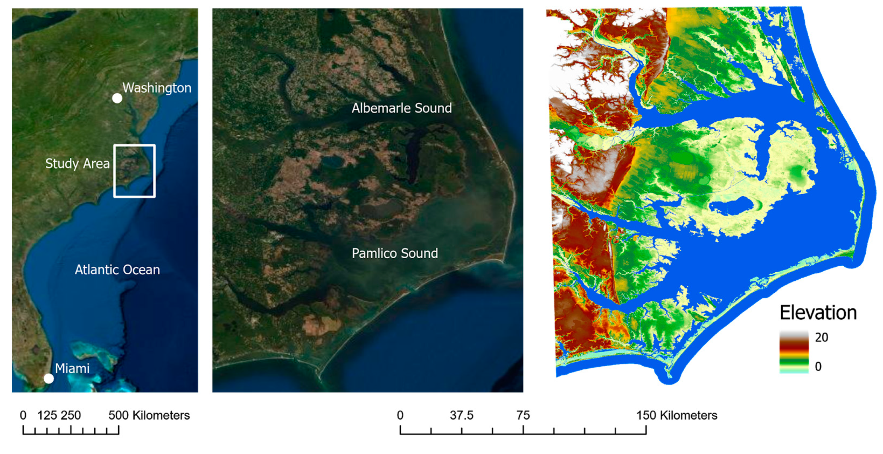
2.1. Study Area
2.2. Data
2.2.1. Satellite Imagery
2.2.2. Training, Validation, and Test Data
2.2.3. LiDAR Data
2.3. Classification Methods
3. Results
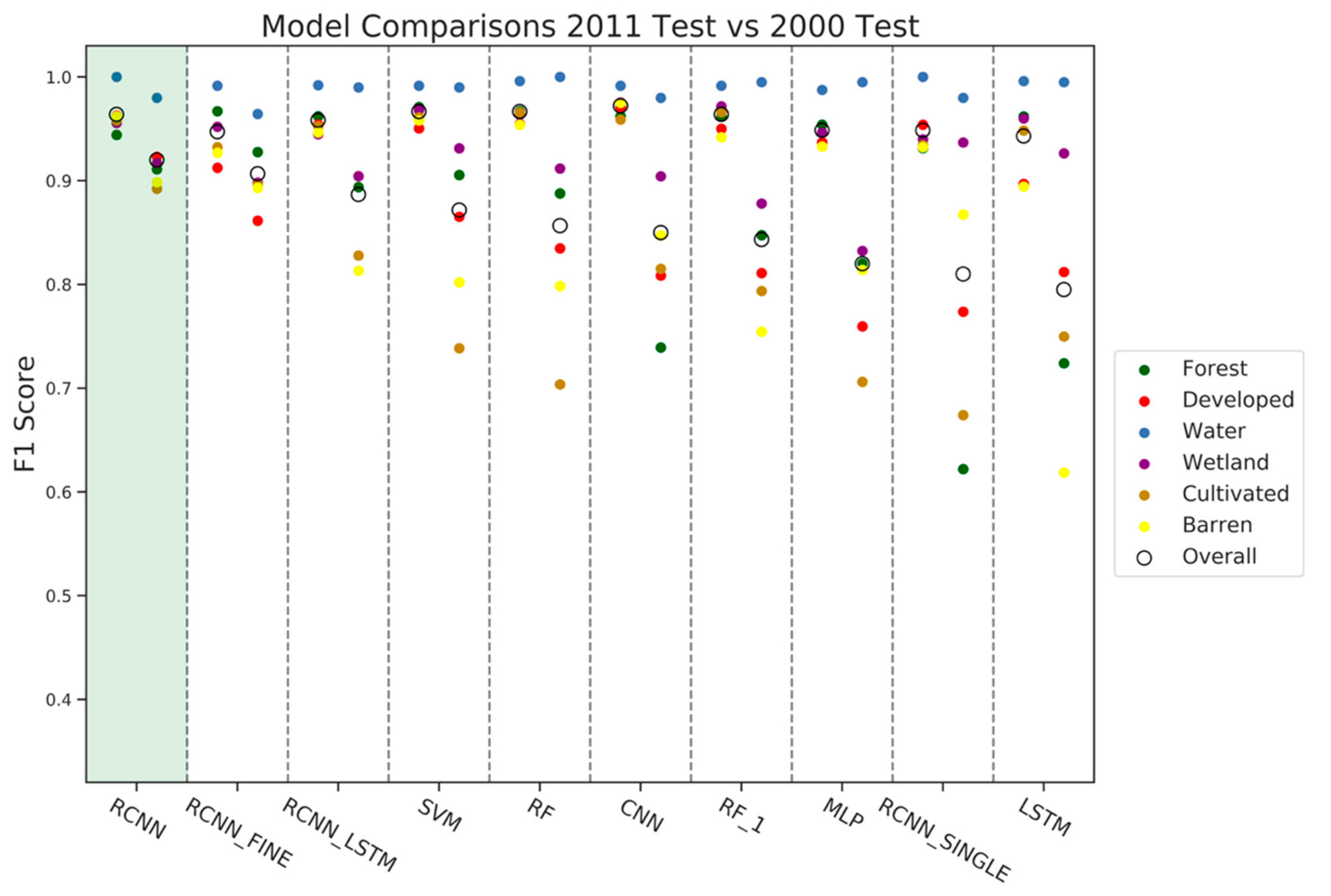
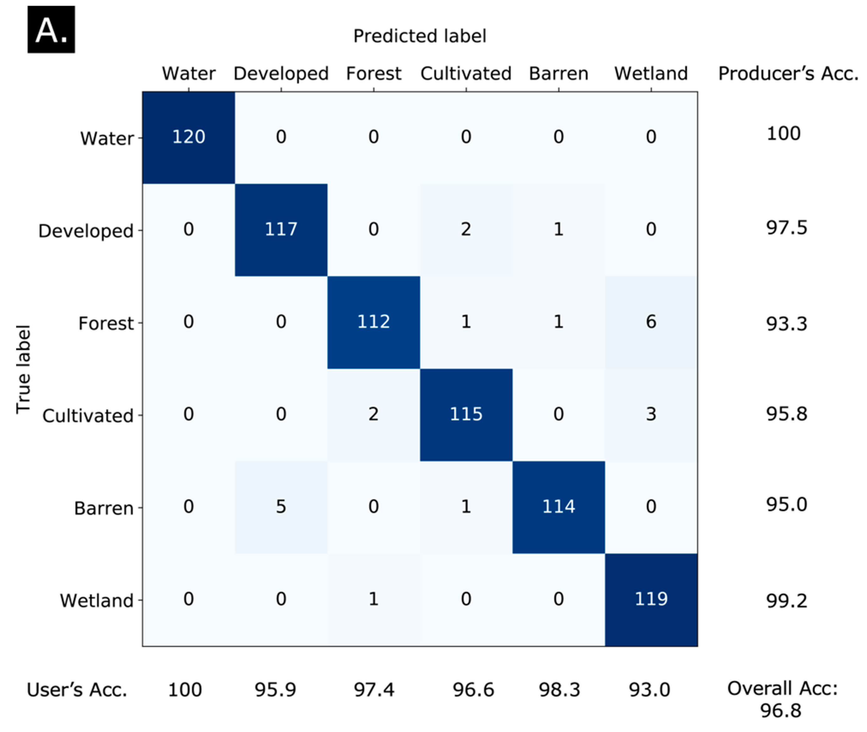
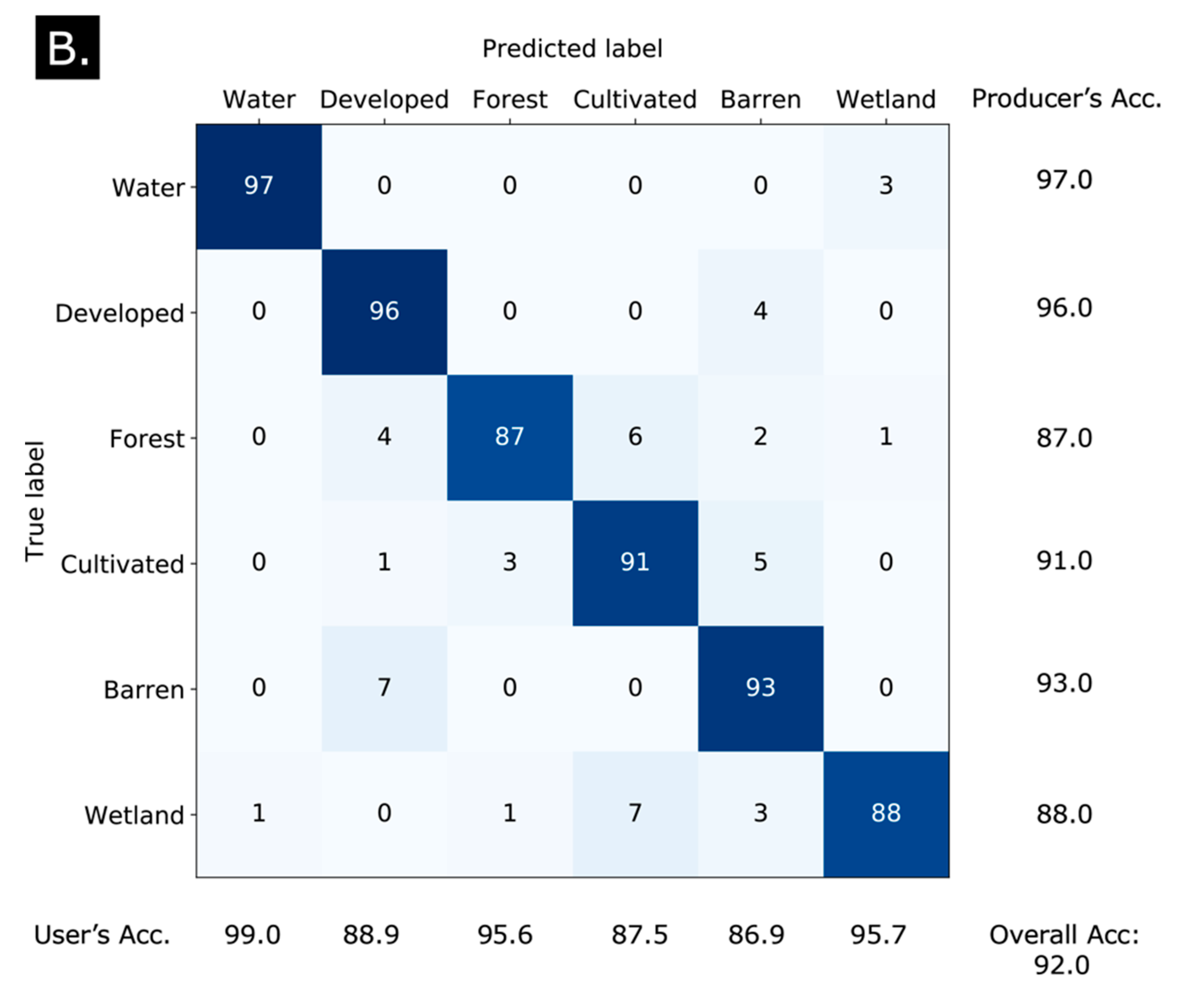
3.1. Model Results
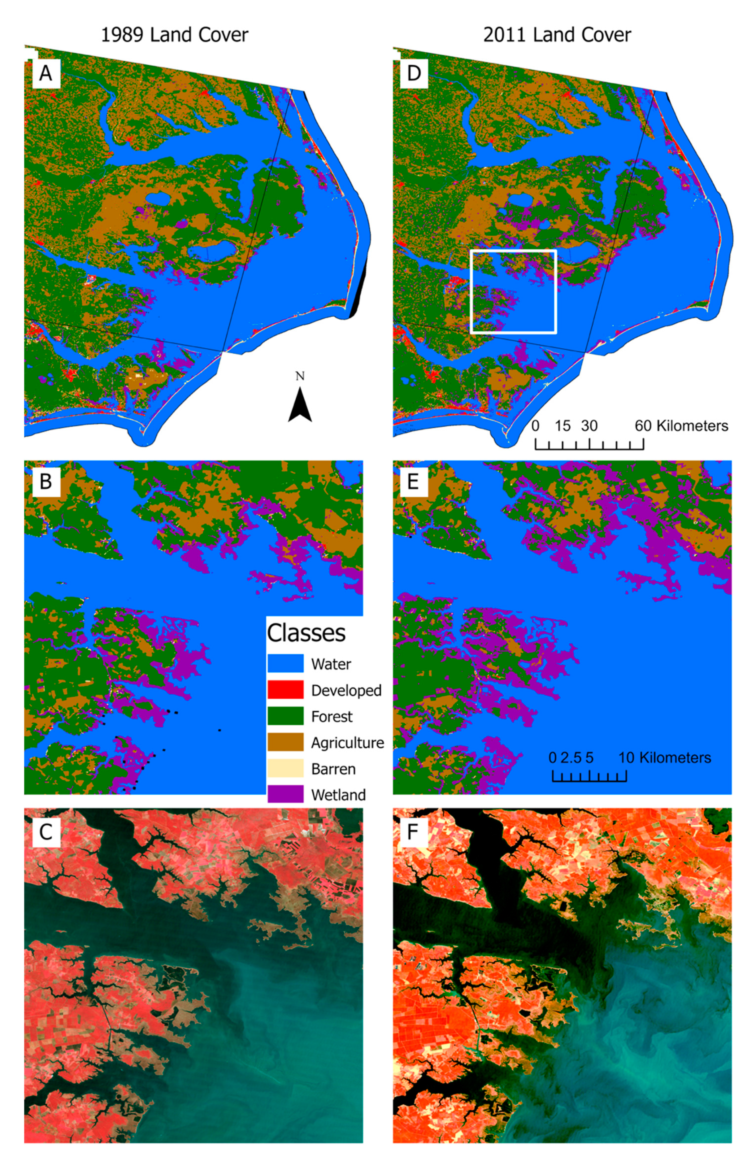
3.2. Ecological Results
4. Discussion
4.1. Implications of Ecological Change
4.2. Data Issues, Labels, and Noise
4.3. Class Separability
4.4. Future Methodological Work
5. Conclusions
Supplementary Materials
Author Contributions
Funding
Data Availability Statement
Acknowledgments
Conflicts of Interest
References
- Huang, C.; Anderegg, W.R.L.; Asner, G.P. Remote sensing of forest die-off in the Anthropocene: From plant ecophysiology to canopy structure. Remote Sens. Environ. 2019, 231, 111233. [Google Scholar] [CrossRef]
- Kirwan, M.L.; Gedan, K.B. Sea-level driven land conversion and the formation of ghost forests. Nat. Clim. Chang. 2019, 9, 450–457. [Google Scholar] [CrossRef] [Green Version]
- Bonan, G.B. Forests and climate change: Forcings, feedbacks, and the climate benefits of forests. Science 2008, 320, 1444–1449. [Google Scholar] [CrossRef] [Green Version]
- Patterson, T.M.; Coelho, D.L. Ecosystem services: Foundations, opportunities, and challenges for the forest products sector. For. Ecol. Manag. 2009, 257, 1637–1646. [Google Scholar] [CrossRef]
- DeFries, R.; Asner, G.P.; Barford, C.; Bonan, G.; Carpenter, S.R.; Chapin, F.S.; Coe, M.T.; Daily, G.C.; Gibbs, H.K.; Helkowski, J.H.; et al. Global consequences of land use. Science 2005, 309, 570. [Google Scholar]
- Juárez, R.I.N.; Chambers, J.Q.; Zeng, H.; Baker, D.B. Hurricane driven changes in land cover create biogeophysical climate feedbacks. Geophys. Res. Lett. 2008, 35, 3–7. [Google Scholar] [CrossRef]
- Kalnay, E.; Cai, M. Impact of urbanization and land-use change on climate. Nature 2003, 423, 528–531. [Google Scholar] [CrossRef]
- Noss, R.F.; Platt, W.J.; Sorrie, B.A.; Weakley, A.S.; Means, D.B.; Costanza, J.; Peet, R.K. How global biodiversity hotspots may go unrecognized: Lessons from the North American Coastal Plain. Divers. Distrib. 2015, 21, 236–244. [Google Scholar] [CrossRef]
- Bhattachan, A.; Emanuel, R.E.; Ardón, M.; Bernhardt, E.S.; Anderson, S.M.; Stillwagon, M.G.; Ury, E.A.; BenDor, T.K.; Wright, J.P. Evaluating the effects of land-use change and future climate change on vulnerability of coastal landscapes to saltwater intrusion. Elementa 2018, 6, 62. [Google Scholar] [CrossRef] [Green Version]
- Riggs, S.R.; Ames, D.V. Drowning the North Carolina coast: Sea-Level Rise and Estuarine Dynamics; North Carolina Sea Grant: Morehead City, NC, USA, 2003; ISBN 0-9747801-0-3. [Google Scholar]
- Brown, J.F.; Tollerud, H.J.; Barber, C.P.; Zhou, Q.; Dwyer, J.L.; Vogelmann, J.E.; Loveland, T.R.; Woodcock, C.E.; Stehman, S.V.; Zhu, Z.; et al. Lessons learned implementing an operational continuous United States national land change monitoring capability: The Land Change Monitoring, Assessment, and Projection (LCMAP) approach. Remote Sens. Environ. 2020, 238, 111356. [Google Scholar] [CrossRef]
- Gómez, C.; White, J.C.; Wulder, M.A. Optical remotely sensed time series data for land cover classification: A review. ISPRS J. Photogramm. Remote Sens. 2016, 116, 55–72. [Google Scholar] [CrossRef] [Green Version]
- Wulder, M.A.; Coops, N.C.; Roy, D.P.; White, J.C.; Hermosilla, T. Land cover 2.0. Int. J. Remote Sens. 2018, 39, 4254–4284. [Google Scholar] [CrossRef] [Green Version]
- Zhu, Z. Change detection using landsat time series: A review of frequencies, preprocessing, algorithms, and applications. ISPRS J. Photogramm. Remote Sens. 2017, 130, 370–384. [Google Scholar] [CrossRef]
- Sexton, J.O.; Urban, D.L.; Donohue, M.J.; Song, C. Long-term land cover dynamics by multi-temporal classification across the Landsat-5 record. Remote Sens. Environ. 2013, 128, 246–258. [Google Scholar] [CrossRef]
- Kennedy, R.E.; Yang, Z.; Cohen, W.B. Detecting trends in forest disturbance and recovery using yearly Landsat time series: 1. LandTrendr—Temporal segmentation algorithms. Remote Sens. Environ. 2010, 114, 2897–2910. [Google Scholar] [CrossRef]
- Zhu, Z.; Zhang, J.; Yang, Z.; Aljaddani, A.H.; Cohen, W.B.; Qiu, S.; Zhou, C. Continuous monitoring of land disturbance based on Landsat time series. Remote Sens. Environ. 2020, 238, 111116. [Google Scholar] [CrossRef]
- Homer, C.; Dewitz, J.; Jin, S.; Xian, G.; Costello, C.; Danielson, P.; Gass, L.; Funk, M.; Wickham, J.; Stehman, S.; et al. Conterminous United States land cover change patterns 2001–2016 from the 2016 National Land Cover Database. ISPRS J. Photogramm. Remote Sens. 2020, 162, 184–199. [Google Scholar] [CrossRef]
- Jin, S.; Homer, C.; Yang, L.; Danielson, P.; Dewitz, J.; Li, C.; Zhu, Z.; Xian, G.; Howard, D. Overall methodology design for the United States national land cover database 2016 products. Remote Sens. 2019, 11, 2971. [Google Scholar] [CrossRef] [Green Version]
- Woodcock, C.E.; Macomber, S.A.; Pax-Lenney, M.; Cohen, W.B. Monitoring large areas for forest change using Landsat: Generalization across space, time and Landsat sensors. Remote Sens. Environ. 2001, 78, 194–203. [Google Scholar] [CrossRef] [Green Version]
- Gray, J.; Song, C. Consistent classification of image time series with automatic adaptive signature generalization. Remote Sens. Environ. 2013, 134, 333–341. [Google Scholar] [CrossRef]
- Fraser, R.H.; Olthof, I.; Pouliot, D. Monitoring land cover change and ecological integrity in Canada’s national parks. Remote Sens. Environ. 2009, 113, 1397–1409. [Google Scholar] [CrossRef]
- Olthof, I.; Butson, C.; Fraser, R. Signature extension through space for northern landcover classification: A comparison of radiometric correction methods. Remote Sens. Environ. 2005, 95, 290–302. [Google Scholar] [CrossRef]
- Kerner, H.R.; Sahajpal, R.; Skakun, S.; Becker-Reshef, I.; Barker, B.; Hosseini, M.; Puricelli, E.I.; Gray, P. Resilient In-Season Crop Type Classification in Multispectral Satellite Observations using Growth Stage Normalization. In Proceedings of the Association for Computing Machinery Knowledge Discovery and Data Mining, San Diego, CA, USA, 23–27 August 2020. [Google Scholar]
- Zeng, L.; Wardlow, B.D.; Xiang, D.; Hu, S.; Li, D. A review of vegetation phenological metrics extraction using time-series, multispectral satellite data. Remote Sens. Environ. 2020, 237, 111511. [Google Scholar] [CrossRef]
- Pouliot, D.; Latifovic, R.; Zabcic, N.; Guindon, L.; Olthof, I. Development and assessment of a 250m spatial resolution MODIS annual land cover time series (2000–2011) for the forest region of Canada derived from change-based updating. Remote Sens. Environ. 2014, 140, 731–743. [Google Scholar] [CrossRef]
- Stehman, S.V.; Foody, G.M. Key issues in rigorous accuracy assessment of land cover products. Remote Sens. Environ. 2019, 231, 111199. [Google Scholar] [CrossRef]
- Chang, T.; Rasmussen, B.P.; Dickson, B.G.; Zachmann, L.J. Chimera: A multi-task recurrent convolutional neural network for forest classification and structural estimation. Remote Sens. 2019, 11, 768. [Google Scholar] [CrossRef] [Green Version]
- Lecun, Y.; Bengio, Y.; Hinton, G. Deep learning. Nature 2015, 521, 436–444. [Google Scholar] [CrossRef] [PubMed]
- Ma, L.; Liu, Y.; Zhang, X.; Ye, Y.; Yin, G.; Johnson, B.A. Deep learning in remote sensing applications: A meta-analysis and review. ISPRS J. Photogramm. Remote Sens. 2019, 152, 166–177. [Google Scholar] [CrossRef]
- Kussul, N.; Lavreniuk, M.; Skakun, S.; Shelestov, A. Deep Learning Classification of Land Cover and Crop Types Using Remote Sensing Data. IEEE Geosci. Remote Sens. Lett. 2017, 14, 778–732. [Google Scholar] [CrossRef]
- Zhu, X.X.; Tuia, D.; Mou, L.; Xia, G.-S.; Zhang, L.; Xu, F.; Fraundorfer, F. Deep Learning in Remote Sensing: A Comprehensive Review and List of Resources. IEEE Geosci. Remote Sens. Mag. 2017, 5, 8–36. [Google Scholar] [CrossRef] [Green Version]
- He, K.; Zhang, X.; Ren, S.; Sun, J. Deep Residual Learning for Image Recognition. Comput. Vis. Pattern Recognit. (CVPR) 2016, 770–778. [Google Scholar] [CrossRef] [Green Version]
- Krizhevsky, A.; Sutskever, I.; Hinton, G.E. ImageNet Classification with Deep Convolutional Neural Networks. Adv. Neural Inf. Process. Syst. 2017, 60, 84–90. [Google Scholar] [CrossRef]
- Long, J.; Shelhamer, E.; Darrell, T. Fully convolutional networks for semantic segmentation. In Proceedings of the IEEE Conference on Computer Vision and Pattern Recognition, Boston, MA, USA, 7–12 June 2015; pp. 3431–3440. [Google Scholar] [CrossRef] [Green Version]
- Graves, A.; Mohamed, A.R.; Hinton, G. Speech recognition with deep recurrent neural networks. In Proceedings of the ICASSP, IEEE International Conference on Acoustics, Speech and Signal Processing, Vancouver, BC, Canada, 26–31 May 2013. [Google Scholar]
- Wan, J.; Wang, D.; Hoi, S.C.H.; Wu, P.; van Merrienboer, B.; Bahdanau, D.; Dumoulin, V.; Serdyuk, D.; Warde-farley, D.; Chorowski, J.; et al. A Critical Review of Recurrent Neural Networks for Sequence Learning. Int. J. Comput. Vis. 2015, arXiv:1207.0580. [Google Scholar]
- Brodrick, P.G.; Davies, A.B.; Asner, G.P. Uncovering Ecological Patterns with Convolutional Neural Networks. Trends Ecol. Evol. 2019, 34, 734–745. [Google Scholar] [CrossRef]
- Ridge, J.T.; Gray, P.C.; Windle, A.E.; Johnston, D.W. Deep learning for coastal resource conservation: Automating detection of shellfish reefs. Remote Sens. Ecol. Conserv. 2020, 6, 431–440. [Google Scholar] [CrossRef]
- Weinstein, B.G.; Marconi, S.; Bohlman, S.; Zare, A.; White, E. Individual Tree-Crown Detection in RGB Imagery Using Semi-Supervised Deep Learning Neural Networks. Remote Sens. 2019, 11, 1309. [Google Scholar] [CrossRef] [Green Version]
- Maggiori, E.; Tarabalka, Y.; Charpiat, G.; Alliez, P. Convolutional Neural Networks for Large-Scale Remote Sensing Image Classification. IEEE Trans. Geosci. Remote Sens. 2017, 55, 645–657. [Google Scholar] [CrossRef] [Green Version]
- Mahdianpari, M.; Salehi, B.; Rezaee, M.; Mohammadimanesh, F.; Zhang, Y. Very deep convolutional neural networks for complex land cover mapping using multispectral remote sensing imagery. Remote Sens. 2018, 10, 1119. [Google Scholar] [CrossRef] [Green Version]
- Ismail Fawaz, H.; Forestier, G.; Weber, J.; Idoumghar, L.; Muller, P.A. Deep learning for time series classification: A review. Data Min. Knowl. Discov. 2019, 33, 917–963. [Google Scholar] [CrossRef] [Green Version]
- Zhong, L.; Hu, L.; Zhou, H. Deep learning based multi-temporal crop classification. Remote Sens. Environ. 2019, 221, 430–443. [Google Scholar] [CrossRef]
- Mou, L.; Ghamisi, P.; Zhu, X.X. Deep recurrent neural networks for hyperspectral image classification. IEEE Trans. Geosci. Remote Sens. 2017, 55, 3639–3655. [Google Scholar] [CrossRef] [Green Version]
- Ienco, D.; Gaetano, R.; Dupaquier, C.; Maurel, P. Land Cover Classification via Multitemporal Spatial Data by Deep Recurrent Neural Networks. IEEE Geosci. Remote Sens. Lett. 2017, 14, 1685–1689. [Google Scholar] [CrossRef] [Green Version]
- Ho Tong Minh, D.; Ienco, D.; Gaetano, R.; Lalande, N.; Ndikumana, E.; Osman, F.; Maurel, P. Deep Recurrent Neural Networks for Winter Vegetation Quality Mapping via Multitemporal SAR Sentinel-1. IEEE Geosci. Remote Sens. Lett. 2018, 15, 465–468. [Google Scholar] [CrossRef]
- Rubwurm, M.; Korner, M. Temporal Vegetation Modelling Using Long Short-Term Memory Networks for Crop Identification from Medium-Resolution Multi-spectral Satellite Images. In Proceedings of the IEEE Conference on Computer Vision and Pattern Recognition Workshops, Honolulu, HI, USA, 21–26 July 2017; pp. 1496–1504. [Google Scholar] [CrossRef]
- Rußwurm, M.; Krner, M. Multi-temporal land cover classification with sequential recurrent encoders. ISPRS Int. J. Geo-Inf. 2018, 7, 129. [Google Scholar] [CrossRef] [Green Version]
- Shi, X.; Chen, Z.; Wang, H.; Yeung, D.Y.; Wong, W.K.; Woo, W.C. Convolutional LSTM network: A machine learning approach for precipitation nowcasting. In Proceedings of the Advances in Neural Information Processing Systems, Montreal, QC, Canada, 7–12 December 2015. [Google Scholar]
- Shi, W.; Zhang, M.; Zhang, R.; Chen, S.; Zhan, Z. Change detection based on artificial intelligence: State-of-the-art and challenges. Remote Sens. 2020, 12, 1688. [Google Scholar] [CrossRef]
- Ienco, D.; Interdonato, R.; Gaetano, R.; Ho Tong Minh, D. Combining Sentinel-1 and Sentinel-2 Satellite Image Time Series for land cover mapping via a multi-source deep learning architecture. ISPRS J. Photogramm. Remote Sens. 2019, 158, 11–22. [Google Scholar] [CrossRef]
- Ouahabi, A.; Taleb-Ahmed, A. Deep learning for real-time semantic segmentation: Application in ultrasound imaging. Pattern Recognit. Lett. 2021, 144, 27–34. [Google Scholar] [CrossRef]
- Lin, T.Y.; Goyal, P.; Girshick, R.; He, K.; Dollar, P. Focal Loss for Dense Object Detection. In Proceedings of the IEEE International Conference on Computer Vision, Venice, Italy, 22–29 October 2017; pp. 2999–3007. [Google Scholar]
- Rußwurm, M.; Körner, M. Self-attention for raw optical Satellite Time Series Classification. ISPRS J. Photogramm. Remote Sens. 2020, 169, 421–435. [Google Scholar] [CrossRef]
- Sainte Fare Garnot, V.; Landrieu, L.; Giordano, S.; Chehata, N. Satellite image time series classification with pixel-set encoders and temporal self-attention. Proc. IEEE Comput. Soc. Conf. Comput. Vis. Pattern Recognit. 2020, 12322–12331. [Google Scholar] [CrossRef]
- Khan, S.; Naseer, M.; Hayat, M.; Zamir, S.W.; Khan, F.S.; Shah, M. Transformers in Vision: A Survey. arXiv Prepr. 2021, arXiv:2101.01169. [Google Scholar]
- Kerner, H.R.; Wagstaff, K.L.; Bue, B.D.; Gray, P.C.; Iii, J.F.B.; Amor, H. Ben Toward Generalized Change Detection on Planetary Surfaces with Convolutional Autoencoders and Transfer Learning. IEEE J. Sel. Top. Appl. Earth Obs. Remote Sens. 2019, 12, 3900–3918. [Google Scholar] [CrossRef]
- Ury, E.A.; Yang, X.; Wright, J.P.; Bernhardt, E.S. Rapid deforestation of a coastal landscape driven by sea level rise and extreme events. Ecol. Appl. 2021, 31, e02339. [Google Scholar] [CrossRef] [PubMed]
- Schieder, N.W.; Kirwan, M.L. Sea-level driven acceleration in coastal forest retreat. Geology 2019, 47, 1151–1155. [Google Scholar] [CrossRef]
- Williams, K.; Ewel, K.C.; Stumpf, R.P.; Putz, F.E.; Workman, T.W. Sea-level rise and coastal forest retreat on the west coast of Florida, USA. Ecology 1999, 80, 2045–2063. [Google Scholar] [CrossRef]
- White, E.; Kaplan, D. Restore or retreat? Saltwater intrusion and water management in coastal wetlands. Ecosyst. Health Sustain. 2017, 3, e12580. [Google Scholar] [CrossRef] [Green Version]
- Ury, E.A.; Anderson, S.M.; Peet, R.K.; Bernhardt, E.S.; Wright, J.P. Succession, regression and loss: Does evidence of saltwater exposure explain recent changes in the tree communities of North Carolina’s Coastal Plain? Ann. Bot. 2020, 125, 255–264. [Google Scholar] [CrossRef] [Green Version]
- Dwyer, J.L.; Roy, D.P.; Sauer, B.; Jenkerson, C.B.; Zhang, H.K.; Lymburner, L. Analysis ready data: Enabling analysis of the landsat archive. Remote Sens. 2018, 10, 1363. [Google Scholar] [CrossRef]
- Masek, J.G.; Vermote, E.F.; Saleous, N.E.; Wolfe, R.; Hall, F.G.; Huemmrich, K.F.; Gao, F.; Kutler, J.; Lim, T.K. A landsat surface reflectance dataset for North America, 1990–2000. IEEE Geosci. Remote Sens. Lett. 2006, 3, 68–72. [Google Scholar] [CrossRef]
- USGS Landsat Analysis Ready Data (ARD) Level-2 Data Product. Available online: https://www.usgs.gov/centers/eros/science/usgs-eros-archive-landsat-archives-us-landsat-analysis-ready-data-ard-level-2?qt-science_center_objects=0#qt-science_center_objects (accessed on 18 August 2020).
- Egorov, A.V.; Roy, D.P.; Zhang, H.K.; Li, Z.; Yan, L.; Huang, H. Landsat 4, 5 and 7 (1982 to 2017) Analysis Ready Data (ARD) observation coverage over the conterminous United States and implications for terrestrial monitoring. Remote Sens. 2019, 11, 447. [Google Scholar] [CrossRef] [Green Version]
- Qiu, S.; Lin, Y.; Shang, R.; Zhang, J.; Ma, L.; Zhu, Z. Making Landsat time series consistent: Evaluating and improving Landsat analysis ready data. Remote Sens. 2019, 11, 51. [Google Scholar] [CrossRef] [Green Version]
- Homer, C.; Dewitz, J.; Yang, L.; Jin, S.; Danielson, P.; Xian, G.; Coulston, J.; Herold, N.; Wickham, J.; Megown, K. Completion of the 2011 national land cover database for the conterminous United States—Representing a decade of land cover change information. Photogramm. Eng. Remote Sens. 2015, 81, 345–354. [Google Scholar] [CrossRef]
- Wickham, J.; Stehman, S.V.; Gass, L.; Dewitz, J.A.; Sorenson, D.G.; Granneman, B.J.; Poss, R.V.; Baer, L.A. Thematic accuracy assessment of the 2011 National Land Cover Database (NLCD). Remote Sens. Environ. 2017, 191, 328–341. [Google Scholar] [CrossRef] [Green Version]
- Gray, P.C.; Ridge, J.T.; Poulin, S.K.; Seymour, A.C.; Schwantes, A.M.; Swenson, J.J.; Johnston, D.W. Integrating drone imagery into high resolution satellite remote sensing assessments of estuarine environments. Remote Sens. 2018, 10, 1257. [Google Scholar] [CrossRef] [Green Version]
- Pedregosa, F.; Varoquaux, G.; Gramfort, A.; Michel, V.; Thirion, B.; Grisel, O.; Blondel, M.; Prettenhofer, P.; Weiss, R.; Dubourg, V.; et al. Scikit-learn: Machine learning in Python. J. Mach. Learn. Res. 2011, 12, 2825–2830. [Google Scholar]
- Chollet, F. Keras: The Python Deep Learning library. Available online: https://keras.io/.
- Huang, G.; Liu, Z.; Van Der Maaten, L.; Weinberger, K.Q. Densely connected convolutional networks. In Proceedings of the 30th IEEE Conference on Computer Vision and Pattern Recognition, CVPR, Honolulu, HI, USA, 21–26 July 2017. [Google Scholar]
- Tajbakhsh, N.; Shin, J.Y.; Gurudu, S.R.; Hurst, R.T.; Kendall, C.B.; Gotway, M.B.; Liang, J. Convolutional Neural Networks for Medical Image Analysis: Full Training or Fine Tuning? IEEE Trans. Med. Imaging 2016, 35, 1299–1312. [Google Scholar] [CrossRef] [Green Version]
- Yosinski, J.; Clune, J.; Bengio, Y.; Lipson, H. How transferable are features in deep neural networks? In Proceedings of the Advances in Neural Information Processing Systems, Montreal, QC, Canada, 8–13 December 2014; pp. 1–9. [Google Scholar]
- Pratt, J.H. Drainage of North Carolina Swamp Lands. J. Elisha Mitchell Sci. Soc. 1909, 25, 158–163. [Google Scholar]
- Manda, A.K.; Giuliano, A.S.; Allen, T.R. Influence of artificial channels on the source and extent of saline water intrusion in the wind tide dominated wetlands of the southern Albemarle estuarine system (USA). Environ. Earth Sci. 2014, 79, 4409–4419. [Google Scholar] [CrossRef]
- Manda, A.K.; Reyes, E.; Pitt, J.M. In situ measurements of wind-driven salt fluxes through constructed channels in a coastal wetland ecosystem. Hydrol. Process. 2018, 32, 636–643. [Google Scholar] [CrossRef]
- Tully, K.; Gedan, K.; Epanchin-Niell, R.; Strong, A.; Bernhardt, E.S.; Bendor, T.; Mitchell, M.; Kominoski, J.; Jordan, T.E.; Neubauer, S.C.; et al. The invisible flood: The chemistry, ecology, and social implications of coastal saltwater intrusion. Bioscience 2019, 69, 368–378. [Google Scholar] [CrossRef]
- Moorhead, K.K.; Brinson, M.M. Response of wetlands to rising sea level in the lower coastal plain of North Carolina. Ecol. Appl. 1995, 5, 261–271. [Google Scholar] [CrossRef]
- Schieder, N.W. Reconstructing Coastal Forest Retreat and Marsh Migration Response to Historical Sea Level Rise; College of William and Mary: Williamsburg, VA, USA, 2018. [Google Scholar]
- Spencer, T.; Schuerch, M.; Nicholls, R.J.; Hinkel, J.; Lincke, D.; Vafeidis, A.T.; Reef, R.; McFadden, L.; Brown, S. Global coastal wetland change under sea-level rise and related stresses: The DIVA Wetland Change Model. Glob. Planet. Chang. 2016. [Google Scholar] [CrossRef] [Green Version]
- Kirwan, M.L.; Temmerman, S.; Skeehan, E.E.; Guntenspergen, G.R.; Fagherazzi, S. Overestimation of marsh vulnerability to sea level rise. Nat. Clim. Chang. 2016, 6, 253–260. [Google Scholar] [CrossRef]
- Raabe, E.A.; Stumpf, R.P. Expansion of Tidal Marsh in Response to Sea-Level Rise: Gulf Coast of Florida, USA. Estuaries Coasts 2016, 39, 145–157. [Google Scholar] [CrossRef]
- Cowart, L.; Walsh, J.P.; Corbett, D.R. Analyzing Estuarine Shoreline Change: A Case Study of Cedar Island, North Carolina. J. Coast. Res. 2010, 265, 817–830. [Google Scholar] [CrossRef]
- Theuerkauf, E.J.; Stephens, J.D.; Ridge, J.T.; Fodrie, F.J.; Rodriguez, A.B. Carbon export from fringing saltmarsh shoreline erosion overwhelms carbon storage across a critical width threshold. Estuar. Coast. Shelf Sci. 2015, 164, 367–378. [Google Scholar] [CrossRef]
- Smith, C.S.; Rudd, M.E.; Gittman, R.K.; Melvin, E.C.; Patterson, V.S.; Renzi, J.J.; Wellman, E.H.; Silliman, B.R. Coming to terms with living shorelines: A scoping review of novel restoration strategies for shoreline protection. Front. Mar. Sci. 2020, 7, 434. [Google Scholar] [CrossRef]
- Lester, S.E.; Dubel, A.K.; Hernán, G.; McHenry, J.; Rassweiler, A. Spatial Planning Principles for Marine Ecosystem Restoration. Front. Mar. Sci. 2020, 7, 328. [Google Scholar] [CrossRef]
- Ridge, J.T.; Johnston, D.W. Unoccupied Aircraft Systems (UAS) for Marine Ecosystem Restoration. Front. Mar. Sci. 2020, 7, 438. [Google Scholar] [CrossRef]
- Ren, S.; He, K.; Girshick, R.; Sun, J. Faster R-CNN: Towards Real-Time Object Detection with Region Proposal Networks. IEEE Trans. Pattern Anal. Mach. Intell. 2017, 39, 1137–1149. [Google Scholar] [CrossRef] [Green Version]
- Weinstein, B.G.; Marconi, S.; Bohlman, S.A.; Zare, A.; White, E.P. Cross-site learning in deep learning RGB tree crown detection. Ecol. Inform. 2020, 56, 101021. [Google Scholar] [CrossRef]
- Claverie, M.; Ju, J.; Masek, J.G.; Dungan, J.L.; Vermote, E.F.; Roger, J.C.; Skakun, S.V.; Justice, C. The Harmonized Landsat and Sentinel-2 surface reflectance data set. Remote Sens. Environ. 2018, 219, 145–161. [Google Scholar] [CrossRef]


| Date Order | 1989 | 2000 | 2011 | |
|---|---|---|---|---|
| Tile 028012 | 1 | 1988-12-05 | 2000-01-05 | 2011-01-03 |
| 2 | 1989-03-11 | 2000-04-10 | 2011-03-08 | |
| 3 | 1989-04-12 | 2000-08-16 | 2011-07-30 | |
| 4 | 1989-10-05 | 2000-10-03 | 2011-08-31 | |
| 5 | 1989-10-21 | 2000-10-19 | 2011-11-03 | |
| Tile 029011 | 1 | 1989-03-11 | 2000-02-22 | 2011-01-03 |
| 2 | 1989-04-28 | 2000-04-10 | 2011-03-08 | |
| 3 | 1989-06-15 | 2000-08-16 | 2011-07-30 | |
| 4 | 1989-10-05 | 2000-10-03 | 2011-08-31 | |
| 5 | 1989-10-21 | 2000-10-19 | 2011-10-18 | |
| Tile 028011 | 1 | 1989-03-11 | 2000-01-21 | 2011-01-03 |
| 2 | 1989-04-12 | 2000-04-10 | 2011-03-08 | |
| 3 | 1989-06-15 | 2000-05-12 | 2011-08-31 | |
| 4 | 1989-10-05 | 2000-08-16 | 2011-10-18 | |
| 5 | 1989-10-21 | 2000-10-19 | 2011-11-03 |
| Dataset | Sample Count (per Class) | Filter Process |
|---|---|---|
| 2011 Train | 1500 | Homogeneity filter only |
| 2011 Validation | 120 | Manual validation |
| 2011 Test | 120 | Manual validation |
| 2000 Test | 100 | Manual validation |
| Layer (Type) | Output Shape | Param |
|---|---|---|
| tile_input (InputLayer) | (None, 5, 9, 9, 7) | 0 |
| conv_lst_m2d_1 (ConvLSTM2D) | (None, 5, 7, 7, 64) | 163,840 |
| conv_lst_m2d_2 (ConvLSTM2D) | (None, 5, 5, 64) | 295,168 |
| max_pooling2d_1 | (MaxPooling2 (None, 3, 3, 64) | 0 |
| flatten_1 (Flatten) | (None, 576) | 0 |
| dense_1 (Dense) | (None, 64) | 36,928 |
| landcover (Dense) | (None, 6) | 390 |
| Water 1989 | Developed 1989 | Forest 1989 | Farm 1989 | Barren 1989 | Wetland 1989 | 2011 Totals | Percent Change | |
|---|---|---|---|---|---|---|---|---|
| Water 2011 | 459 | 1 | 5 | 10 | 8 | 14 | 498 | −0.02% |
| Developed 2011 | 3 | 203 | 52 | 52 | 43 | 2 | 355 | 3.87% |
| Forest 2011 | 3 | 25 | 8079 | 1009 | 58 | 62 | 9236 | −1.95% |
| Farm 2011 | 1 | 79 | 582 | 3936 | 93 | 16 | 4707 | −9.79% |
| Barren 2011 | 15 | 21 | 41 | 38 | 116 | 8 | 239 | −33.43% |
| Wetland 2011 | 18 | 12 | 660 | 173 | 42 | 617 | 1520 | 111.40% |
| 1989 Totals | 498 | 341 | 9419 | 5218 | 359 | 719 | 16,554 |
Publisher’s Note: MDPI stays neutral with regard to jurisdictional claims in published maps and institutional affiliations. |
© 2021 by the authors. Licensee MDPI, Basel, Switzerland. This article is an open access article distributed under the terms and conditions of the Creative Commons Attribution (CC BY) license (https://creativecommons.org/licenses/by/4.0/).
Share and Cite
Gray, P.C.; Chamorro, D.F.; Ridge, J.T.; Kerner, H.R.; Ury, E.A.; Johnston, D.W. Temporally Generalizable Land Cover Classification: A Recurrent Convolutional Neural Network Unveils Major Coastal Change through Time. Remote Sens. 2021, 13, 3953. https://0-doi-org.brum.beds.ac.uk/10.3390/rs13193953
Gray PC, Chamorro DF, Ridge JT, Kerner HR, Ury EA, Johnston DW. Temporally Generalizable Land Cover Classification: A Recurrent Convolutional Neural Network Unveils Major Coastal Change through Time. Remote Sensing. 2021; 13(19):3953. https://0-doi-org.brum.beds.ac.uk/10.3390/rs13193953
Chicago/Turabian StyleGray, Patrick Clifton, Diego F. Chamorro, Justin T. Ridge, Hannah Rae Kerner, Emily A. Ury, and David W. Johnston. 2021. "Temporally Generalizable Land Cover Classification: A Recurrent Convolutional Neural Network Unveils Major Coastal Change through Time" Remote Sensing 13, no. 19: 3953. https://0-doi-org.brum.beds.ac.uk/10.3390/rs13193953