Automatic Features Detection in a Fluvial Environment through Machine Learning Techniques Based on UAVs Multispectral Data

Abstract

The present work aims to demonstrate how machine learning (ML) techniques can be used for automatic feature detection and extraction in fluvial environments. The use of photogrammetry and machine learning algorithms has improved the understanding of both environmental and anthropic issues. The developed methodology was applied considering the acquisition of multiple photogrammetric images thanks to unmanned aerial vehicles (UAV) carrying multispectral cameras. These surveys were carried out in the Salbertrand area, along the Dora Riparia River, situated in Piedmont (Italy). The authors developed an algorithm able to identify and detect the water table contour concerning the landed areas: the automatic classification in ML found a valid identification of different patterns (water, gravel bars, vegetation, and ground classes) in specific hydraulic and geomatics conditions. Indeed, the RE+NIR data gave us a sharp rise in terms of accuracy by about 11% and 13.5% of F1-score average values in the testing point clouds compared to RGB data. The obtained results about the automatic classification led us to define a new procedure with precise validity conditions.

1. Introduction

Automatic detection is one of the primary challenges in fluvial environments, especially where spatio-temporal coverage and recognition of fluvial and aquatic topography, hydraulics, geomorphology, and habitat quality are required. Mapping flood water using remote sensing observation technologies is a common practice today, assisting emergency services as well as informing flood mitigation strategies, especially when Sentinel satellite images [1] or synthetic aperture radar (SAR) data [2,3,4,5] are considered. Satellite data are very useful resources for extracting information on very large areas and, when necessary, analysing phenomena that cannot be studied using only contemporary data (e.g., anthropogenic impacts or effects of climate change) and which cause fluvial adjustment [6] but are not sufficient to provide information necessary for high-resolution applications (centimetre scale).

The use of unmanned aerial vehicles (UAVs) has completely changed monitoring approaches and is quite common today due to their low cost, ease of use, and strong performance. As widely described in the literature [7,8], these instruments make it possible to assemble different sensors (such as LiDAR or digital cameras) in order to obtain high-resolution imagery (up to centimetre resolution) and/or dense 3D point clouds. UAVs are quite interesting because they can cover a large area in a very short time (ca. 40 ha/h) and acquire data more rapidly and less expensively than typical airborne surveys, even if the amount of data acquired and their resolution strictly depend on the used UAV platform, the camera sensors on board, as well as the flight height and speed.

Although the use of LiDAR aerial data is rather limited due to the cost of this technology, the recent large-scale diffusion and use of UAVs in various geoscience disciplines has been facilitated by the rapid progress in photogrammetric processing methods without sacrificing accuracy in the final product. In most cases, UAVs are equipped with RGB [9] sensors, sometimes associated with sensors working on different wavelengths, such as near-infrared (NIR) ones, enabling it to obtain images [10]. Then, using a photogrammetric approach, three-dimensional (3D) point clouds can be automatically generated. This approach allows the production of several digital surface models (DSMs), digital terrain models (DTMs) [11], orthophotos [12], and vegetation indices. Thus, fluvial environment monitoring is often possible, as these outcomes enable not only the detection of different environments (such as flooded or aquatic areas as well as vegetation or sandy/rocky regions) [8] but also the classification of different types of soils, vegetation detection [13], and feature extraction, such as tree height, canopy area and diameter [14], and individual tree counting [15].

In the last decade, these tools have gained widespread application. UAVs were originally mainly used for regional research, such as territory analysis, landslide monitoring [16,17], geothermal environments [18], geomorphological studies [19,20,21], and sedimentation [22].

One of the main applications of UAVs in hydrological research is in stream and riverscape mapping due to their ability to rapidly acquire accurate and detailed spatial data, represented by orthophotos and DSMs [23,24]. Detailed mapping of stream properties using UAVs is of special importance for hydromorphological research because objective spatial information can be obtained, particularly for the classification of physical river habitat applications [25] or the analysis of the dynamics of water stages [26]. Moreover, UAV technology can be considered efficient (even if slightly limited) for hydromorphological feature detection [27] (i.e., as described in Langhammer (2018) [28]).

The importance of 3D reconstruction using UAV-based photogrammetry is increasing in fluvial geomorphology, as it allows both quantitative analysis of changes in stream and riparian zones at multitemporal scales and volumetric analyses of bank erosion and fluvial deposition [29,30]. In order to achieve these goals and to be able to analyse medium-scale products, it is necessary to ensure the acquisition of aerial images with a ground sample distance (GSD) of a few centimetres, which affects the generated 3D point clouds and, consequently, the other products [31]. Therefore, careful acquisition planning is required, as the GSD is affected by the image resolution, the camera characteristics, and the acquisition distance from the studied object.

However, one of the main limitations regarding hydrological applications of UAV-based mapping is typically the use of RGB sensors, which limits possibilities to detect and reconstruct the properties of the submerged stream channel, as was well-described in [32,33]. Indeed, “invisible” spectral data (red-edge and near-infrared bands) represent a tremendous step forward in defining environmental, forestry, and hydraulic problems, as thoroughly demonstrated in [34,35,36,37,38]. On the other hand, the use of UAV in shallow riverbeds has provided good performance in stream hydromorphology mapping, enabling partial coverage of submerged zones of the channel [39].

A number of recent studies demonstrated the power of UAV for the analysis of stream planform changes, though most were limited to detection and analysis of fluvial morphologic changes in streams after flooding [40,41] or delimiting flood-prone areas based on DEM analysis [42]. A different approach to detecting the refraction correction problem in a water table was reported in [43].

As the fluvial environment is very complex and made up of different features of nature, in recent years, the academic community has been involved in the study of methodologies for the automatic extraction of different types of information from high resolution data [44]. The literature contains many classification studies from the environmental field using different UAV-integrated sensors or satellite data in order to better recognise vegetation and the water table in fluvial or lake environments, such as [45,46,47]. To solve the classification problem, several studies exploit artificial intelligence methods [48] based on machine learning (ML) algorithms and deep learning methods, thus relying on convolutional neural network architectures. Previous works demonstrated the ability and the good accuracy of these approaches in the classification process, especially in extremely heterogeneous environments [49,50], such as the fluvial ones.

Usually, the features classification in fluvial scenes is based on the exploitation of the satellite images [51] or of orthophotos obtained from photogrammetric image processing [52,53]. This technique can be more advantageous when, due to certain conditions (for example, dense vegetation and the presence of wind during image acquisition), the three-dimensional point cloud, generated during the photogrammetric process, is highly noisy; on the contrary, the direct analysis of the point cloud preserves spatial and three-dimensional information of the scene, allowing one to delimit more accurately the different features and to obtain additional structural information [13].

From the earliest studies on the classification of river environments based on remotely sensed data, the scientific community has highlighted the usefulness of multispectral and hyperspectral sensors [54]. Today, small versions are widely used in the market, even low-cost versions, and can be easily integrated into UAV to replace RGB cameras. The spectral information made available by these sensors makes it possible to greatly improve classification operations as reported in [55]. For example, wavelengths in the near-infrared, not penetrating water, make watercourses easier to be identified with respect to the terrestrial features, while changes in chlorophyll content are emphasized in the spectral range of the red-edge band, supporting the identification of vegetated areas [56].

Thus, this paper aimed to develop an innovative methodology for automatic detection of water table and emerged areas in fluvial environments through machine learning (ML) techniques using UAV RE+NIR spectral data. To generate an innovative product, we developed a script capable of identifying the water table contour with respect to the emerged areas through the automatic classification of RE+NIR 3D point clouds as water, vegetation, and ground/gravel bars. The code was based on a specific modified ML algorithm: the random forest algorithm (RF). The choice of RF was due to its faster setting and processing time, higher classification accuracy, more flexibility in different statistical data type analysis (for example, about supervised classification and unsupervised learning), and more efficient methodology in variable importance evaluation compared to other ML algorithms (such as support vector machine or decision tree) or neural networks. Moreover, it is capable of avoiding the missing values [57,58]. All these characteristics make it preferable in environmental classification problems. Besides, the RF is based on multiple decision trees, which makes it suitable even for large datasets as long as the data have the variability and the diversity necessary to make the classifier transposable to numerous situations in order to strictly reduce the overfitting problems.

2. Study Area

This research project is part of research activity on hydraulic characterisation, planned in the Salbertrand area, to monitor the meso-habitat of aquatic plants in wetlands. The watercourse investigated is the Dora Riparia river near the municipality of Salbertrand in the Alta Val di Susa (also called “Alta Valle della Dora”), which belongs to the metropolitan city of Turin. The investigated section is located between the easternmost section of the dam on the natural course of the Dora Riparia River and the eastern limit of the Salbertrand urban centre, including the entire alluvial plain below the viaduct of the A32–E70 Turin-Bardonecchia highway (Figure 1).

From a particle size standpoint, the alluvial plain is composed of stratified gravel and gravelly-sandy deposits with rounded pebbles in an overlapping arrangement and subordinate blocks. In particular, there are alternations in the coarser levels, from pluri-decimetric to pluri-metric, between gravel and gravel with silty sand and finer levels of comparable thickness composed of silty sands and sandy silts. From the geomorphological point of view, the area is part of the Oulx-Salbertrand plain, a flat valley floor area representing a sector of greater sedimentation by the main watercourses whose deposits are interspersed with the imposing fans fed from the tributary basins. The riverbed in this stretch has a braided-like fluvial pattern.

3. Materials and Methods

The methodology used and proposed here is based on consolidated geomatics technologies in the environmental field associated with the development of algorithms and models for the wet area’s prediction using machine learning techniques (Figure 2).

3.1. Field Survey

To obtain a correct definition of the automatic classification parameters in the fluvial environment of wet areas, high-resolution RE+NIR raster data were employed. The photogrammetric products used as input data for the proposed methodology were realised employing UAV technology. The choice of the aerial platform and the optical sensor for a specific aerial survey depends both on environmental conditions, such as the extension of the study area, its shape, the presence of human-made objects, and other boundary conditions, and on the resolution of the products to be generated. As stated above, radiometric information relating to the visible part of the electromagnetic spectrum alone (corresponding to red, green, and blue bands) is not sufficient to reconstruct the properties of the submerged stream channel [32,33]. Indeed, among spectral bands, the combination of NIR (near infrared) and RE (red-edge) information proved to be the most useful for distinguishing bodies of water, soil, and vegetation moisture [59]. Due to the large area involved and the need for a multispectral optical sensor, we used a Phantom 4 Multispectral commercial multi-rotor solution. The primary feature that made this drone particularly suitable for this research was the integrated multispectral camera equipped with five optical sensors corresponding to red, green, blue, red-edge, and NIR bands, respectively.

Table 1. Phantom 4 Multispectral characteristics.

Phantom 4 Multispectral
	Optical sensors specifications
	Sensors: CMOS 1/2.9″–2.08 MP Images Res.: 1600 × 1300 Focal lengths: 5.74 mm	Filters
		B: 450 nm ± 16 nm
		G: 560 nm ± 16 nm
		R: 650 nm ± 16 nm
		RE: 730 nm ± 16 nm
		NIR: 840 nm ± 26 nm

shows the characteristics of the multispectral camera.

The Phantom 4 Multispectral has a weight of 1.487 kg and a flight autonomy of about 27 min, as specified by the manufacturer.

The entire study area was covered by six flights in clear conditions from 11:00 to 14:00 on 27 July 2020. A total number of 10,332 images (both nadir and oblique) were collected at a height of 40 m, with an average ground resolution of 2 cm and an image overlap of 80% in both directions.

The UAV system employed is also equipped with a multi-constellation multi-frequency GNSS that, through the real-time kinematic (RTK) approach and together with an inertial platform, is able to obtain an accurate position of the centre of the camera and the attitude angles for each captured image. This information allows for direct georeferencing of the photogrammetric block, realising the so-called direct photogrammetry [60]. In this study, to improve the images’ alignment and georeferencing and to check the accuracy of the final 3D model punctually, a number of ground control points (GCPs) and check points (CPs) were surveyed [61]. GCPs and CPs are points with well-known coordinates estimated using different geomatics techniques with accuracies of a few mm or cm. To this end, before performing flights, 38 photographic stable points spread over the study area and easily recognisable in the pictures were identified; 25 were used as GCPs while the other 13 were employed to evaluate georeferencing accuracy (Figure 3). Their position was measured using Leica GS14 and GS18 receivers, exploiting the GNSS NRTK (network real time kinematic) positioning technique and considering the virtual reference station (VRS) correction broadcasted by the SPIN3 GNSS network [62], as described in [63]. The coordinates of the points were estimated with centimetre accuracy (≅3 cm) with fixed-phase ambiguities for all points, ensuring a high level of precision for the georeferencing process.

The GNSS-RTK technique acquires the ellipsoid heights of the measured points, which necessarily must be converted into orthometric heights. These conversions were carried out through the ConverGo software and the use of GK2 grids distributed by the Italian Military Geographical Institute (IGMI), which contain the so-called “geoid undulations” according to the ITALGEO 2005 model. The ETRF2000 (2008.0) with the UTM 32N projection was adopted as the reference system for the project according to the Italian directives.

3.2. Multispectral UAV Data Processing

The aerial image acquisition aimed to produce an orthomosaic for each available band, namely R, G, B, RE, and NIR. The raw data acquired by the multispectral camera in each shot consisted of six images corresponding to the five bands and the RGB band composition; thus, at the end of the acquisition operation for each band, a dataset of 1722 images was obtained. The UAV data were processed using the structure from motion (SfM) approach [64] with the help of commercial software. In this study, the photogrammetric process was carried out using AMP’s commercial solution (Agisoft Metashape Professional). The six datasets were processed in different AMP projects considering both nadir and oblique images.

In the first step of the procedure, the frames were aligned through automatic recognition of the homologous points between two or more images, which enabled the computing of the relative position of the frames in the photogrammetric block as well as the internal camera parameters. The output of the image alignment was a scattered point cloud generated by setting up the “high” level of accuracy of AMP. As previously mentioned, the images were acquired through a UAV-RTK configuration and were already georeferenced. However, in order to optimise the estimation of the camera’s interior parameters and to improve the generation of the photogrammetric block, the coordinates of the measured GCPs and CPs were imported and manually collimated in the images in which they were found. The CPs were used to evaluate the accuracy achieved in the georeferencing phase, resulting in a total residual error of less than 8 cm in each chunk, while we obtained a residual error for the GCPs lower than 5 cm.

Subsequently, each dataset was further processed in order to compute the three-dimensional dense point clouds. A “high” level of detail was selected to obtain products suitable for medium/large-scale investigations (1:500), and “moderate” depth filtering was selected to remove noise due to the presence of dense vegetation.

The next step involved generating a dense digital surface model (DDSM) of the entire study area. We decided to create a single DDSM from the dense point cloud obtained using only the data from the RGB dataset. In fact, this was the densest point cloud as compared with the other datasets and described the model with the highest level of resolution. The density of the 3D information enabled the realisation of a DDSM characterised by a pixel size equal to 8 cm.

The final raster products (i.e., multispectral orthophotos) were generated to realise the basic dataset for the ML detection to be described. The multispectral orthomosaics were computed separately for each band used—red, green, blue, red-edge, and NIR—starting from the previously computed DDSM. Based on the accuracy of the DDSM, orthomosaics with resolutions of 8 cm were produced using the “mosaic” blending mode option on AMP. It was then possible to obtain the composite bands orthomosaic (RE and NIR) by combining the respective single band orthomosaics. Several representative testing rasters were created by the multispectral-composed orthophotos mentioned above in order to evaluate the automatic classification methodology described in Section 3.3. The areas to be used for producing the training (ca. 30% of the whole dataset) and the test datasets (2 sub-datasets corresponding to the ca. 60% of the complete one) were selected based on the areal distribution of the three main desired classes (water, vegetation, and ground/gravel bars) through observation of the orthophotos. The purpose of this visual analysis was to obtain datasets as homogeneous as possible that best discretised the investigated fluvial environment. Figure 4 shows a sketch of the test raster used.

3.3. Automatic Detection of Submerged Areas Using ML Algorithm

To achieve the fundamental aim of this research work, a specific multi-step methodology was developed to define the wet areas of the investigated watercourse.

By exploiting the rate (i.e., reflectance) existing between the incident energy from an electromagnetic source (such as the sun) and the quantity of energy reflected by a surface or object (i.e., radiance), it is possible to identify the spectral signature characteristic of the object detected [65]. In the multispectral approach, different spectral signatures are obtained for each detected band, increasing the identification capacity of the investigated surfaces. The multispectral sensor acquires the radiance signal coming from the reflecting surface, converting it into a digital signal and subsequently recording in the form of a digital number (DN) matrix. Hence, the spectral signature is none other than the reflectance extended to the entire measurable spectrum. From the analysis of the RE and the NIR spectra, three main classes were defined: (i) water, characterized by lower reflectance; (ii) vegetation, having higher and variable reflectance values in the two aforementioned bands; (iii) ground and gravel bars, with medium intensity in RE-NIR spectra.

The radiance values observed allowed developing an innovative methodology for automatic classification using ML algorithms.

To obtain strong results in classifying fluvial environments, we were properly focalised on the river system, which is composed of a water table, gravel bars, and wide wooded areas. Thus, the datasets were buffered 50–75 m from the watercourse. In order to evaluate the RE + NIR classification goodness, we compared the RE + NIR and the RGB band classified clouds, as shown in the Results section. The following ML steps were carried out on both types of spectral data.

The first step was the conversion of the orthophotos into points, extracting the RE + NIR data. The use of open and free GIS platforms is important to this process due to their widespread application in a variety of professional and academic fields and is a key factor in reducing costs. The last stable release of QGIS software–3.16.1 “Hannover” [66]—was used with the integrated Grass 7.8.4 module. Data preparation processing was developed to obtain three representative test datasets, described below:

• First, for every dataset, a composite orthophoto was built, merging together the RE and NIR bands, and grouped into a single composite orthophotos using a specific command in QGIS software called “Merge”.
• Second, the composite orthophotos were converted in point clouds and assigned the RE-NIR true values at each point. To realized it, we used the “Raster pixels to points” command, obtaining some representative clouds of the Salbertrand area. Additionally, longitude and latitude coordinates were assigned and set to the ETRF2000-UTM32N coordinates system. Then, we assigned at the clouds the RE-NIR values extracting the information by the stacked pixels of the composite orthomosaics using a specific plugin in QGIS software (Point Sampling tool).
• Finally, the test datasets generated were exported in text format with integer values.

Next, to obtain an accurate training dataset, a segmentation step was required in addition to those described above. Three specific groups of points (named ROI—region of interest) were manually noted. The obtained ROIs represent the three desired classes: water [11], vegetation [22], and ground/gravel bars [33], as shown in Figure 5.

The automatic classification proposed here focused on developing all-encompassing ML code through the free programming language Python (latest version 3.9.1) [67]. This particular code-writing platform implements many different free and open problem-solving scripts and libraries available online, which are used to read several kinds of formats (such as text or shapefile) or conduct various mathematical and logical processes. For our purposes, we chose various logical classification libraries (i.e., NumPy, Pandas, SciPy, and Matplotlib) [68,69,70,71] to achieve a complete ML codebase. The random forest (RF) algorithm was chosen from the ScikitLearn Python library [72]. The RF algorithm comprises a list of exchanging multiple defined decision trees, which minimise overfitting errors.

First, the CV modules were run using cross_val_score [73] and GridSearchCV [74] from Python’s libraries to measure and improve the generalisation capacity performance of the RF algorithm. Figure 6 shows a representative sketch on raw data preparation, cross-validation processing, and optimal parameter evaluation.

Next, the raw data were split into 80% training and 20% test datasets using the train_test_split() function [75], applying the cross_val_score module, which subdivided the training dataset into specified folds (i.e., 4 folds). The function used three folds to train the model (training set) and the fourth for validation (validation set), iterating this process four times (iterations 1,2,3,4) while changing the pairs of training–validation folds.

As shown in Figure 6, four CV accuracy values were calculated on the validation set—one for each iteration. Additionally, the statistical parameters of precision, recall, and F1-score were computed [76] to obtain an overview of the initial generalisation power of the chosen RF algorithm. These parameters were based on the relationships between true positive (Tp), false positive (Fp), true negative (Tn), and false negative (Fn) values obtained from the confusion matrix. These accuracy parameters are shown below:

$$\begin{gathered} \mathrm{Accuracy}\mathrm{Score}=\frac{{\mathrm{y}}_{\mathrm{testing}}}{{\mathrm{y}}_{\mathrm{training}}} \\ \mathrm{Precision}=\frac{{\mathrm{t}}_{\mathrm{p}}}{{\mathrm{t}}_{\mathrm{p}}+{\mathrm{f}}_{\mathrm{f}}} \\ \mathrm{Recall}=\frac{{\mathrm{t}}_{\mathrm{p}}}{{\mathrm{t}}_{\mathrm{p}}+{\mathrm{f}}_{\mathrm{n}}} \\ \mathrm{F}1-\mathrm{score}=\frac{2\ast \mathrm{Precion}\ast \mathrm{Recall}}{\mathrm{Precision}+\mathrm{Recall}} \end{gathered}$$

(1)

where y_testing and y_training contain the predicted and the ground-truth data, respectively.

The developed code computes the CV standard deviation as well, returning a very low variance value (<1%).

Table 2. Parameters obtained during the CV iterations.

	Iteration 1	Iteration 2	Iteration 3	Iteration 4
Accuracy	0.98	0.98	0.98	0.98
Precision	0.97	0.96	0.96	0.96
Recall	0.97	0.97	0.97	0.97
F1-score	0.97	0.97	0.97	0.97
Standard deviation	0.0000992
Time (mm:ss)	7:18

summarises the results obtained.

It was then possible to evaluate the optimal combination of RF algorithm hyperparameters to perform the classification as best as possible. The GridSearchCV module tests every combination of values of the defined hyperparameters, training the model and calculating the accuracy of the test dataset. Through the functions best_params_ and best_score_, we printed the best combination of hyperparameters and its accuracy score. More information regarding the RF hyperparameters can be found in [77].

Table 3. GridSearchCV proceeding for RF best parameter’s evaluation.

RF Hyperparameters	Value 1	Value 2	Value 3	Best_Params_	Best_Score	Time (hh:mm)
n_estimators	10	25	50	criterion: ‘gini’
criterion	Gini	entropy	-	max_features: ‘auto’
max_features	Auto	Log2	-	min_samples_leaf: 10
min_samples_split	5	7	10	min_samples_split: 10
min_samples_leaf	4	6	10	n_estimators: 50
random_state	None	0	42	random_state: None

shows the chosen hyperparameters and their assigned values as well as the ideal combination (subsequently used to classify the second and the third point clouds) and its accuracy score.

It is important to note the lengthy processing time and the computational load (core running at 100% of CPU for nearly 10 h) of this cross-validation step due to the high number of tested combinations (324) and the large size of the trained dataset (over 2,500,000 points).

The step-by-step ML classification procedure is briefly summarised below. For further information, please reference the GitHub repository [78] available online and reported in the Supplementary Materials Section.

• Importing and organizing training/test datasets. To organise a proof-reading ML algorithm, training and test datasets were imported into Python script. If the datasets were large, it was possible to toggle off the low_memory function (see the Pandas libraries for more detailed information at [69]). The training dataset was then split into RE-NIR feature columns and a labelled class through a proper expression, recalling and assigning them in Features and Labels subfolders. Moreover, the test dataset contained only the RE+NIR spectral features; thus, it was possible to call them into the script.
• Preprocessing of the training dataset. In order to improve classification accuracy, the training dataset was processed, setting the threshold affected by the minimum number of the points value of the classes (11, 22, and 33 in this paper) to obtain more balanced datasets [79,80]. Furthermore, the balanced training dataset was randomised [81,82].
• Model’s training and classification of test dataset. The random forest algorithm, comprising the RandomForestClassifier module [77], was chosen to classify the external test dataset. The optimal hyperparameters obtained during the GridSearchCV processing were set.
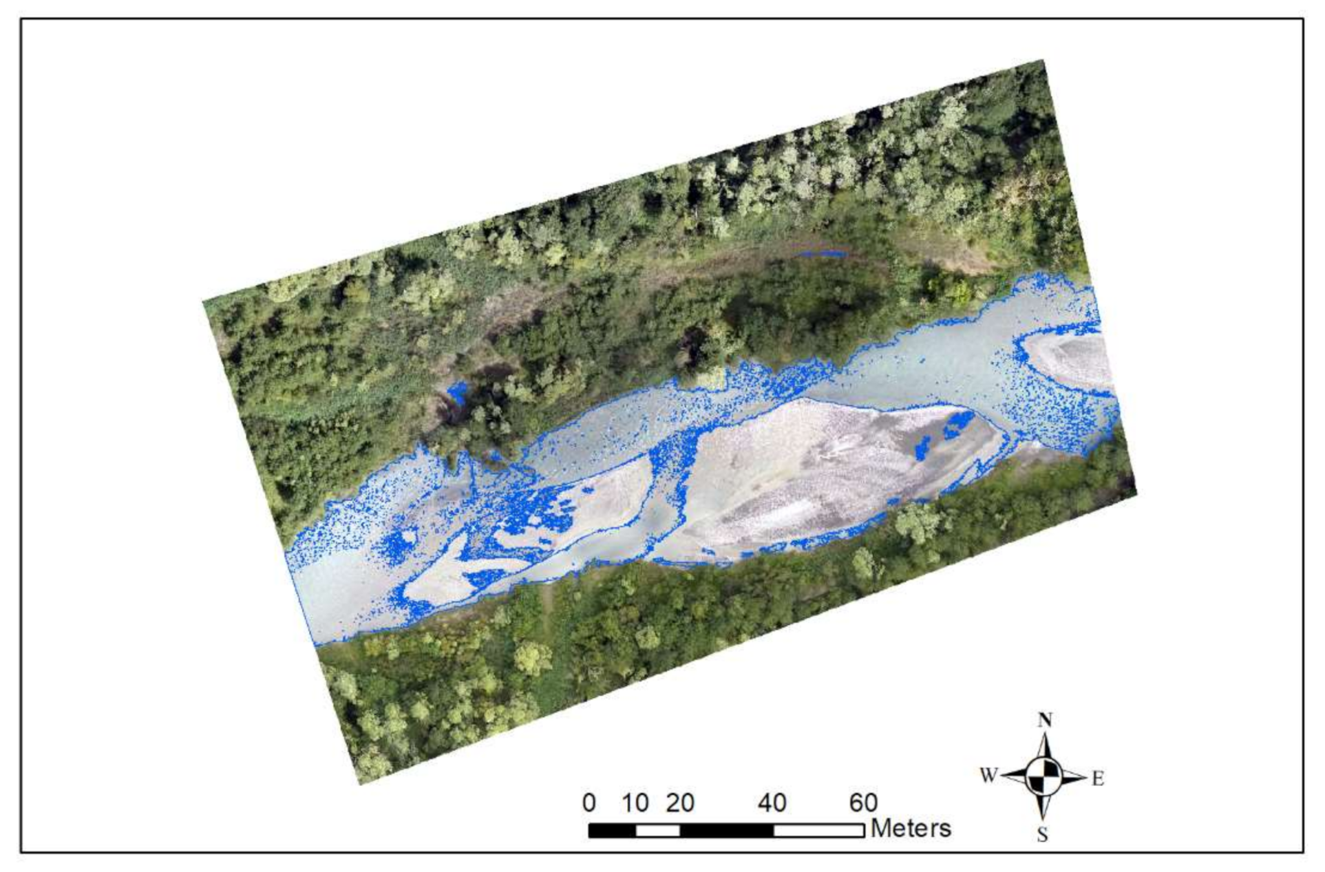
• Saving and exporting the test dataset. Finally, the classified test datasets were exported, assigning the points’ coordinates again to the resulting class itself (water, vegetation, and ground/gravel bars, respectively). The classified dense point clouds obtained are shown in Figure 7.

The ML classification code was not complete; it was necessary to run several functions to evaluate the classification’s goodness. For testing classified clouds (second and third clouds), accuracy score, precision, recall, F1-score, and confusion matrix parameters were computed, comparing the obtained values from the RE+NIR classification with those of the RGB visible spectrum.

The innovative ML data processing above described, classified, and returned the dense point clouds, assigning a specific value at every output point (water {11}, vegetation {22}, or ground/gravel bars {33}). Another procedure was developed using free and open-source GIS software, such as QGIS, to obtain a more suitable product. First, the classified point clouds were rasterised in order to select and extract only the water class value. Next, to filter and delete eventual erroneous classification points, a polygonisation function was used in order to calculate the wet area of every polygon and eliminate the undesired polygons, with a threshold based on the representative value of the calculated area (i.e., <1 sqm). The final product was a polygon shapefile of the water table enclosed in very precise wet contours in the fluvial environment that was suitable for hydraulic and safety plan purposes, as shown in Figure 8.

4. Results

The identification of wet areas through automatic classification is not a novel concept, as reported by previous studies carried out using different types of instruments, such as radar and satellite [1,2,3,4,5]. The development of UAV-integrated sensor technology has enabled a sharp reduction in the cost of data acquisition [83], making UAV accessibility in environmental monitoring valuable to professionals and organisations.

The drones can be equipped with various sensors capable of better defining the investigated objects. The use of sensors linked to the visible spectrum (RGB) has constituted a major development in recent decades, becoming the standard in photogrammetric data production. However, these sensors may not be accurate enough in specific cases; therefore, UAVs with sensors of different wavelength ranges, such as infrared bands, were used. The use of these bands in the environmental field has grown in recent years, particularly in the monitoring of wooded areas or regions subject to flooding [35,38,39,40].

At the same time, it was necessary to develop an innovative classification methodology based on ML algorithms, which was built by writing a specific script in Python in order to guarantee its complete open access and free availability. The application of this code to the RE+NIR spectral data made it possible to compute statistical parameters regarding model accuracy and generalisation. In order to evaluate the accuracy parameters, we ran the ML classification script on the RGB test datasets as well and obtained the same accuracy parameters.

Table 4. Second classified cloud accuracy parameters obtained.

	Water [11]	Vegetation [22]	Gr_Gb [33]	TOT
RGB accuracy score	-	-	-	0.905
RE+NIR accuracy score	-	-	-	0.987
RGB precision	1.00	0.98	0.60	0.86
RE+NIR precision	0.99	0.99	0.99	0.99
RGB recall	0.74	0.99	0.90	0.88
RE+NIR recall	0.99	1.00	0.93	0.97
RGB F1-score	0.85	0.99	0.72	0.85
RE+NIR F1-score	0.99	0.99	0.96	0.98

and

Table 5. Third classified cloud accuracy parameters obtained.

	Water [11]	Vegetation [22]	Gr_Gb [33]	TOT
RGB accuracy score	-	-	-	0.934
RE+NIR accuracy score	-	-	-	0.953
RGB precision	0.93	0.99	0.72	0.89
RE+NIR precision	0.90	0.98	0.89	0.92
RGB recall	0.79	0.98	0.88	0.89
RE+NIR recall	0.97	0.99	0.77	0.91
RGB F1-score	0.85	0.99	0.80	0.88
RE+NIR F1-score	0.93	0.99	0.83	0.91

and Figure 9 show the main statistical parameters obtained for the second and the third classified clouds (accuracy score, precision, recall, F1-score, and confusion matrix), comparing the RGB and the RE+NIR dataset results.

The spatial distribution data and its percentage were computed to represent the obtained RE-NIR accuracy improvement, as shown in

Table 6. Geometrics values observed, corresponding at RGB and RE+NIR classifications processing.

	Water’s Area (m2)	Vegetation’s Area (m2)	Ground/Gravel Bars (m2)	TOT (m2)
Second cloud:				10,991.67
RGB	1447.57	7213.11	2250.98
RE-NIR	2233.18	7020.49	1657.99
Third cloud:
RGB	2750.87	11,923.27	4727.61	19,361.75
RE-NIR	3872.98	12,006.93	3491.84

and

Table 7. Percentages related on RGB and RE+NIR classifications processing.

	Water’s Classified Points (%)	Vegetation’s Classified Points (%)	Ground/Gravel Bars Classified Points (%)
Second cloud:
RGB	13.26	66.10	20.64
RE-NIR	20.46	64.34	15.20
Third cloud:
RGB	14.05	61.65	24.3
RE-NIR	19.99	61.98	18.02

.

In

Table 8. Overview about square meters errors for every classes: RGB and RE+NIR datasets.

	Water’s Area Error (m2)	Vegetation’s Area Error (m2)	Ground/Gravel Bars Area Error (m2)
Second cloud:
RGB	376.37	72.13	900.39
RE-NIR	22.33	70.2	16.58
Third cloud:
RGB	577.68	112.24	1323.73
RE-NIR	116.34	120.07	384.11

, we attempted to identify the estimates of the errors that occurred in terms of square metres, expressed for each class, multiplying the percentage values of the statistical parameters reported in Table 4 and Table 5 by the classes’ areas shown in Table 6. It is important to note that these values are reported in absolute values.

5. Discussion

The analysis of the results in Table 4 and Table 5 put in evidence large differences in terms of precision and recall regarding the water and the ground/gravel bar. Comparing the classified clouds (second and third, respectively), a significant contamination between the two classes was shown in the RGB datum due to the similarity between their spectral values in semi-submerged areas. Indeed, precision values of 60% and 72% for the ground/gravel bar class and recall percentages equal to 74% and 79% for the water class were obtained. As can be seen in Figure 7, in the watercourse areas that had strong solar reflections or were semi-submerged, the water points were very similar to those of gravel bars in terms of RGB values and were consequently labelled as gravel bars instead of water. This problem did not arise when the RE-NIR bands were used due to the well-defined water ranges of values (as previously described). This was demonstrated by the much higher precision values in the ground/gravel bar class (99% and 89% for the second and the third classified clouds, respectively), while the values assumed by the recall in the water class also showed better percentages (99% and 97%, respectively), verifying the improvement of the water table identification by means of RE+NIR data.

This evidence was also numerically confirmed by the confusion matrices analysis, as shown in Figure 9: over 60,000 and 58,000 wrongly classified points (upper right boxes) from the second and the third RGB datasets, respectively, were reported. Specifically, these points were classified as gravel bars even if submerged. Comparing the same data on the RE+NIR confusion matrices obtained, the values slightly exceeded 6000 units in the worst case, recognising a significant decrease of wet areas classification errors.

Furthermore, in the third classified point cloud, the presence of a dried and vegetated channel tended to increase the value of the false negative of the ground/gravel bars class during classification with RE+NIR data (recall equal to 77%). This suggests that identifying emerging areas should be further investigated, though they were not the main focus of this study.

Next, observing the F1-score harmonic values between RGB and RE+NIR data, increases of 14% and 8% on the second and the third clouds, respectively, were seen. This constitutes further evidence of superior recognition of the water table using RE+NIR data.

From the comparison of the two different classification approaches, as reported in Table 6 and Table 7, in both classified clouds, a significant difference in water’s area coverage was evident, with a lower value from the RGB classifications (1447.57 m² and 2750.87 m²) than from the RE+NIR spectral ones (2233.18 m² and 3872.98 m²). Additionally, analysing the data obtained for the ground/gravel bars class, higher values for the RGB bands (2250.98 m² and 4727.61 m²) as compared to the RE+NIR ones (1657.99 m² and 3491.84 m²) were observed.

The water class identified using the RE+NIR spectral approach had lower areal errors (22.33 m² and 116.34 m²) than the RGB method (376.37 m² and 577.68 m²) for both the second and the third tested datasets. Moreover, the same trend could be observed in ground/gravel bars errors: the RE-NIR classification produced 16.58 m² and 384.11 m² error, an improvement on the 900.39 m² and 1323.73 m² obtained for the RGB classified clouds. Finally, the vegetation class represents an equilibrium between the two, with no substantial variations in areal extensions.

The spatial data reported in Table 6, Table 7 and Table 8, associated with the statistical parameters described in Table 4 and Table 5, suggest an underestimation of the water class using RGB bands, an error that is associated with an overestimation of the ground/gravel bars class. These classification errors were overcome using infrared spectral data, leading to a substantial improvement in the identification of wet areas [84].

The combination of recall and precision values as well as the areal errors described above show how RE and NIR bands greatly reduced underestimation of the wet areas obtained with the RGB bands while, at the same time, correcting the overestimation of the gravel bars.

In conclusion, the results reported here suggest that UAVs equipped with multispectral sensors are preferable to those equipped with cheaper RGB sensors alone, although this upgrade comes with a higher cost.

6. Conclusions

Obtaining an automatic classification in fluvial environments is a major challenge, especially where spatio-temporal coverage and recognition of fluvial and aquatic topography, hydraulics, geomorphology, and habitat quality are needed. Since these changes occur rapidly, it is important to use highly productive and powerful instruments for data acquisition and to develop algorithms to extract information automatically. This paper demonstrated the importance of using multispectral images collected from UAVs for the classification of fluvial environments using ML algorithms. The RE and the NIR bands’ reflectance values seemed to overcome the limitations of the standard RGB radiometry, improving the accuracy of wet area detection. Automatic classification was achieved by developing an innovative methodology based on ad-hoc Python code. The described procedure was applied to alpine watercourses and showed excellent result accuracy and ease of use, as detailed in the Results section. The application of this ML script on RE+NIR spectral point clouds in the Salbertrand region led to a sharp improvement in water table recognition, as shown by the decrease in false positive and false negative values (precision and recall percentages) and the lower errors (in square metres) as compared to the RGB classification. For these reasons, we can assert that RE+NIR data are more discerning than RGB data in identifying wet areas in an alpine watercourse.

The innovation about our ML model is focused on its ease of use and its suitability for every professional and environmental expert for monitoring purposes. Moreover, the code is completely free and open to modify, available online in GitHub repository.

Given the alpine nature of the investigated watercourse, at present, it is appropriate to point out that the predictive model developed is to be tested in the future on larger rivers in order to observe possible limitation in water table detection. Thus, we aim to test the developed methodology in other fluvial environment case studies to validate its usefulness. Furthermore, we would add other features to the training test datasets, such as textures, height values, and specific index (such as that described in [85]) in order to improve our classification results and limit the “projected shadows” as much as possible. The possibility to apply this method in several fluvial environment case studies would represent a great advantage in support of the operations monitoring these areas and preventing catastrophic events that more and more often follow each other because of climate change.

References

1. Bioresita, F.; Puissant, A.; Stumpf, A.; Malet, J.-P. A Method for Automatic and Rapid Mapping of Water Surfaces from Sentinel-1. Imagery. Remote Sens. 2018, 10, 217. [Google Scholar] [CrossRef] [Green Version]
2. Westerhoff, R.S.; Kleuskens, M.P.H.; Winsemius, H.C.; Huizinga, H.J.; Brakenridge, G.R.; Bishop, C. Automated global water mapping based on wide-swath orbital synthetic-aperture radar. Hydrol. Earth Syst. Sci. 2013, 17, 651–663. [Google Scholar] [CrossRef] [Green Version]
3. Martinis, S.; Kersten, J.; Twele, A. A fully automated TerraSAR-X based flood service. ISPRS J. Photogramm. Remote Sens. 2015, 104, 203–212. [Google Scholar] [CrossRef]
4. Pulvirenti, L.; Pierdicca, N.; Chini, M.; Guerriero, L. An algorithm for operational flood mapping from Synthetic Aperture Radar (SAR) data using fuzzy logic. Nat. Hazards Earth Syst. Sci. 2011, 11, 529–540. [Google Scholar] [CrossRef] [Green Version]
5. Giustarini, L.; Hostache, R.; Matgen, P.; Schumann, G.J.-P.; Bates, P.D.; Mason, D.C. A Change Detection Approach to Flood Mapping in Urban Areas Using TerraSAR-X. IEEE Trans. Geosci. Remote Sens. 2012, 51, 2417–2430. [Google Scholar] [CrossRef] [Green Version]
6. Bakker, M.; Lane, S.N. Archival photogrammetric analysis of river-floodplain systems using Structure from Motion (SfM) methods. Earth Surf. Process. Landf. 2016, 42, 1274–1286. [Google Scholar] [CrossRef] [Green Version]
7. Pádua, L.; Vanko, J.; Hruška, J.; Adão, T.; Sousa, J.J.; Peres, E.; Morais, R. UAS, sensors, and data processing in agroforestry: A review towards practical applications. Int. J. Remote Sens. 2017, 38, 2349–2391. [Google Scholar] [CrossRef]
8. Carrivick, J.L.; Smith, M.W. Fluvial and aquatic applications of Structure from Motion photogrammetry and unmanned aer-ial vehicle/drone technology. Wiley Interdiscip. Rev. Water 2019, 6, e1328. [Google Scholar] [CrossRef] [Green Version]
9. Endres, F.; Hess, J.; Sturm, J.; Cremers, D.; Burgard, W. 3-D Mapping With an RGB-D Camera. IEEE Trans. Robot. 2013, 30, 177–187. [Google Scholar] [CrossRef]
10. Chen, S.C.; Hsiao, Y.S.; Chung, T.H. Determination of landslide and driftwood potentials by fixed-wing UAV-borne RGB and NIR images: A case study of Shenmu Area in Taiwan. In Proceedings of the EGU General Assembly Conference Abstracts, Vienna, Austria, 12–17 April 2015; p. 2491. [Google Scholar]
11. Dabove, P.; Manzino, A.M.; Taglioretti, C. The DTM accuracy for hydrological analysis. Geoing. Ambient. Min. 2015, 144, 15–22. [Google Scholar]
12. Guarnieri, A.; Masiero, A.; Vettore, A.; Pirotti, F. Evaluation of the dynamic processes of a landslide with laser scanners and Bayesian methods. Geomat. Nat. Hazards Risk 2014, 6, 614–634. [Google Scholar] [CrossRef] [Green Version]
13. Carbonell-Rivera, J.P.; Estornell, J.; Ruiz, L.A.; Torralba, J.; Crespo-Peremarch, P. Classification of Uav-Based Photogram-metric Point Clouds of Riverine Species Using Machine Learning Algorithms: A Case Study in the Palancia River, Spain. Int. Arch. Photogramm. Remote Sens. Spat. Inf. Sci. 2020, 43, 659–666. [Google Scholar] [CrossRef]
14. Wang, X.; Zhao, Q.; Han, F.; Zhang, J.; Jiang, P. Canopy Extraction and Height Estimation of Trees in a Shelter Forest Based on Fusion of an Airborne Multispectral Image and Photogrammetric Point Cloud. J. Sens. 2021, 2021, 5519629. [Google Scholar] [CrossRef]
15. Dong, X.; Zhang, Z.; Yu, R.; Tian, Q.; Zhu, X. Extraction of Information about Individual Trees from High-Spatial-Resolution UAV-Acquired Images of an Orchard. Remote Sens. 2020, 12, 133. [Google Scholar] [CrossRef] [Green Version]
16. Farfaglia, S.; Lollino, G.; Iaquinta, M.; Sale, I.; Catella, P.; Martino, M.; Chiesa, S. The Use of UAV to Monitor and Manage the Territory: Perspectives from the SMAT Project. In Engineering Geology for Society and Territory-Volume 5; Springer: Cham, Switzerland, 2015; pp. 691–695. [Google Scholar]
17. Torrero, L.; Seoli, L.; Molino, A.; Giordan, D.; Manconi, A.; Allasia, P.; Baldo, M. The Use of Micro-UAV to Monitor Active Landslide Scenarios. In Engineering Geology for Society and Territory-Volume 5; Springer: Cham, Switzerland, 2015; pp. 701–704. [Google Scholar]
18. Nishar, A.; Richards, S.; Breen, D.; Robertson, J.; Breen, B. Thermal infrared imaging of geothermal environments by UAV (un-manned aerial vehicles). J. Unmanned Veh. Syst. 2016, 4, 136–145. [Google Scholar] [CrossRef]
19. Lucieer, A.; de Jong, S.M.; Turner, D. Mapping landslide displacements using structure from motion (SfM) and image corre-lation of multi-temporal UAV photography. Prog. Phys. Geogr. 2013, 38, 97–116. [Google Scholar] [CrossRef]
20. Eltner, A.; Baumgart, P.; Maas, H.-G.; Faust, D. Multi-temporal UAV data for automatic measurement of rill and interrill ero-sion on loess soil. Earth Surf. Process. Landf. 2015, 406, 741–755. [Google Scholar] [CrossRef]
21. Smith, M.W.; Vericat, D. From experimental plots to experimental landscapes: Topography, erosion and deposition in sub-humid badlands from structure-from-motion photogrammetry. Earth Surf. Process. Landf. 2015, 4012, 1656–1671. [Google Scholar] [CrossRef] [Green Version]
22. Wheaton, J.M.; Brasington, J.; Darby, S.E.; Sear, D.A. Accounting for uncertainty in DEMs from repeat topographic surveys: Improved sediment budgets. Earth Surf. Process. Landf. 2009, 35, 136–156. [Google Scholar] [CrossRef]
23. Dietrich, J.T. Riverscape mapping with helicopter-based Structure-from-Motion photogrammetry. Geomorphology 2016, 252, 144–157. [Google Scholar] [CrossRef]
24. Flener, C.; Vaaja, M.; Jaakkola, A.; Krooks, A.; Kaartinen, H.; Kukko, A.; Kasvi, E.; Hyyppä, H.; Hyyppä, J.; Alho, P. Seamless Mapping of River Channels at High Resolution Using Mobile LiDAR and UAV-Photography. Remote Sens. 2013, 5, 6382–6407. [Google Scholar] [CrossRef] [Green Version]
25. Woodget, A.S.; Austrums, R.; Maddock, I.; Habit, E. Drones and digital photogrammetry: From classifications to continuums for monitoring river habitat and hydromorphology. Wiley Interdiscip. Rev. Water 2017, 4. [Google Scholar] [CrossRef] [Green Version]
26. Witek, M.; Jeziorska, J.; Niedzielski, T. An experimental approach to verifying prognoses of floods using an unmanned aerial vehicle. Meteorology Hydrology and Water Management. Res. Oper. Appl. 2014, 21, 3–11. [Google Scholar]
27. Casado, M.R.; Gonzalez, R.B.; Kriechbaumer, T.; Veal, A. Automated identification of river hydromorphological features using UAV high resolution aerial imagery. Sensors 2015, 15, 27969–27989. [Google Scholar] [CrossRef] [PubMed] [Green Version]
28. Langhammer, J.; Vacková, T. Detection and Mapping of the Geomorphic Effects of Flooding Using UAV Photogrammetry. Pure Appl. Geophys. 2018, 175, 3223–3245. [Google Scholar] [CrossRef]
29. Miřijovský, J.; Langhammer, J. Multitemporal monitoring of the morphodynamics of a mid-mountain stream using UAS photogrammetry. Remote Sens. 2015, 7, 8586–8609. [Google Scholar] [CrossRef] [Green Version]
30. Tamminga, A.D.; Eaton, B.C.; Hugenholtz, C.H. UAS-based remote sensing of fluvial change following an extreme flood event. Earth Surf. Process. Landf. 2015, 40, 1464–1476. [Google Scholar] [CrossRef]
31. Neumann, K.J. Trends for digital aerial mapping cameras. Int. Arch. Photogramm. Remote Sens. Spat. Inf. Sci. (ISPRS) 2008, 28, 551–554. [Google Scholar]
32. Lejot, J.; Delacourt, C.; Piégay, H.; Fournier, T.; Trémélo, M.-L.; Allemand, P. Very high spatial resolution imagery for chan-nel bathymetry and topography from an unmanned mapping controlled platform. Earth Surf. Process. Landf. 2007, 32, 1705–1725. [Google Scholar] [CrossRef]
33. Thumser, P.; Kuzovlev, V.V.; Zhenikov, K.Y.; Zhenikov, Y.N.; Boschi, M.; Boschi, P. Using structure from motion (SfM) technique for the characterization of riverine systems—case study in the headwaters of the Volga River. Geogr. Environ. Sustain. 2017, 10, 31–43. [Google Scholar] [CrossRef] [Green Version]
34. Available online: http://www.ricercasit.it/Public/Documenti/1_Rapporto_satelliti_definitivo.pdf (accessed on 21 July 2021).
35. Easterday, K.; Kislik, C.; Dawson, T.E.; Hogan, S.; Kelly, M. Remotely Sensed Water Limitation in Vegetation: Insights from an Experiment with Unmanned Aerial Vehicles (UAVs). Remote Sens. 2019, 11, 1853. [Google Scholar] [CrossRef] [Green Version]
36. Castro, C.C.; Gómez, J.A.D.; Martín, J.D.; Sánchez, B.A.H.; Arango, J.L.C.; Tuya, F.A.C.; Díaz-Varela, R. An UAV and Satellite Multispectral Data Approach to Monitor Water Quality in Small Reservoirs. Remote Sens. 2020, 12, 1514. [Google Scholar] [CrossRef]
37. Li, N.; Martin, A.; Estival, R. An automatic water detection approach based on Dempster-Shafer theory for multi-spectral images. In Proceedings of the 2017 20th International Conference on Information Fusion (Fusion), Xi’an, China, 10–13 July 2017; pp. 1–8. [Google Scholar]
38. Belcore, E.; Wawrzaszek, A.; Wozniak, E.; Grasso, N.; Piras, M. Individual Tree Detection from UAV Imagery Using Hölder Exponent. Remote Sens. 2020, 12, 2407. [Google Scholar] [CrossRef]
39. Woodget, A.S.; Carbonneau, P.E.; Visser, F.; Maddock, I.P. Quantifying submerged fluvial topography using hyperspatial resolution UAS imagery and structure from motion photogrammetry. Earth Surf. Process. Landf. 2014, 40, 47–64. [Google Scholar] [CrossRef] [Green Version]
40. Langhammer, J.; Hartvich, F.; Kliment, Z.; Jeníček, M.; Bernsteinová, J.; Vlček, L.; Su, Y.; Štych, P.; Miřijovský, J. The impact of disturbance on the dynamics of fluvial processes in mountain landscapes. Silva Gabreta 2015, 21, 105–116. [Google Scholar]
41. Langhammer, J.; Lendzioch, T.; Miřijovský, J.; Hartvich, F. UAV-based optical granulometry as tool for detecting changes in structure of flood depositions. Remote Sens. 2017, 9, 240. [Google Scholar] [CrossRef] [Green Version]
42. Şerban, G.; Rus, I.; Vele, D.; Breţcan, P.; Alexe, M.; Petrea, D. Flood-prone area delimitation using UAV technology, in the areas hard-to-reach for classic aircrafts: Case study in the north-east of Apuseni Mountains, Transylvania. Nat. Hazards 2016, 82, 1817–1832. [Google Scholar] [CrossRef]
43. Emanuele, P.; Nives, G.; Andrea, C.; Carlo, C.; Paolo, D.; Maria, L.A. Bathymetric Detection of Fluvial Environments through UASs and Machine Learning Systems. Remote Sens. 2020, 12, 4148. [Google Scholar] [CrossRef]
44. Carbonneau, P.E.; Dugdale, S.J.; Breckon, T.P.; Dietrich, J.T.; Fonstad, M.A.; Miyamoto, H.; Woodget, A.S. Adopting deep learning methods for airborne RGB fluvial scene classification. Remote Sens. Environ. 2020, 251, 112107. [Google Scholar] [CrossRef]
45. Chabot, D.; Dillon, C.; Shemrock, A.; Weissflog, N.; Sager, E.P.S. An Object-Based Image Analysis Workflow for Monitoring Shallow-Water Aquatic Vegetation in Multispectral Drone Imagery. ISPRS Int. J. Geo-Inf. 2018, 7, 294. [Google Scholar] [CrossRef] [Green Version]
46. Sun, F.; Sun, W.; Chen, J.; Gong, P. Comparison and improvement of methods for identifying waterbodies in remotely sensed imagery. Int. J. Remote Sens. 2012, 33, 6854–6875. [Google Scholar] [CrossRef]
47. Dronova, I.; Gong, P.; Wang, L. Object-based analysis and change detection of major wetland cover types and their classification uncertainty during the low water period at Poyang Lake, China. Remote Sens. Environ. 2011, 115, 3220–3236. [Google Scholar] [CrossRef]
48. Chollet, F. Deep Learning with Python; Simon and Schuster: New York, NY, USA, 2017. [Google Scholar]
49. Pouliot, D.; Latifovic, R.; Pasher, J.; Duffe, J. Assessment of Convolution Neural Networks for Wetland Mapping with Landsat in the Central Canadian Boreal Forest Region. Remote Sens. 2019, 11, 772. [Google Scholar] [CrossRef] [Green Version]
50. Mahdianpari, M.; Salehi, B.; Rezaee, M.; Mohammadimanesh, F.; Zhang, Y. Very Deep Convolutional Neural Networks for Complex Land Cover Mapping Using Multispectral Remote Sensing Imagery. Remote Sens. 2018, 10, 1119. [Google Scholar] [CrossRef] [Green Version]
51. Kuhn, C.; Valerio, A.D.M.; Ward, N.; Loken, L.; Sawakuchi, H.O.; Kampel, M.; Richey, J.; Stadler, P.; Crawford, J.; Striegl, R.; et al. Performance of Landsat-8 and Sentinel-2 surface reflectance products for river remote sensing retrievals of chlorophyll-a and turbidity. Remote Sens. Environ. 2019, 224, 104–118. [Google Scholar] [CrossRef] [Green Version]
52. Ren, L.; Liu, Y.; Zhang, S.; Cheng, L.; Guo, Y.; Ding, A. Vegetation Properties in Human-Impacted Riparian Zones Based on Unmanned Aerial Vehicle (UAV) Imagery: An Analysis of River Reaches in the Yongding River Basin. Forests 2020, 12, 22. [Google Scholar] [CrossRef]
53. Van Iersel, W.; Straatsma, M.; Middelkoop, H.; Addink, E. Multitemporal Classification of River Floodplain Vegetation Using Time Series of UAV Images. Remote Sens. 2018, 10, 1144. [Google Scholar] [CrossRef] [Green Version]
54. Carbonneau, P.; Piégay, H. (Eds.) Fluvial Remote Sensing for Science and Management; John Wiley & Sons: Hoboken, NJ, USA, 2012. [Google Scholar]
55. Demarchi, L.; Van De Bund, W.; Pistocchi, A. Object-Based Ensemble Learning for Pan-European Riverscape Units Mapping Based on Copernicus VHR and EU-DEM Data Fusion. Remote Sens. 2020, 12, 1222. [Google Scholar] [CrossRef] [Green Version]
56. Kang, Y.; Meng, Q.; Liu, M.; Zou, Y.; Wang, X. Crop Classification Based on Red Edge Features Analysis of GF-6 WFV Data. Sensors 2021, 21, 4328. [Google Scholar] [CrossRef]
57. Nitze, I.; Schulthess, U.; Asche, H. Comparison of machine learning algorithms random forest, artificial neural network and support vector machine to maximum likelihood for supervised crop type classification. In Proceedings of the 4th GEOBIA, Rio de Janeiro, Brazil, 7–9 May 2012; Volume 35. [Google Scholar]
58. Cutler, D.R.; Edwards, T.C., Jr.; Beard, K.H.; Cutler, A.; Hess, K.T.; Gibson, J.; Lawler, J.J. Random forests for classification in ecology. Ecology 2007, 8811, 2783–2792. [Google Scholar] [CrossRef]
59. Lefebvre, G.; Davranche, A.; Willm, L.; Campagna, J.; Redmond, L.; Merle, C.; Guelmami, A.; Poulin, B. Introducing WIW for Detecting the Presence of Water in Wetlands with Landsat and Sentinel Satellites. Remote Sens. 2019, 11, 2210. [Google Scholar] [CrossRef] [Green Version]
60. Wu, C.; Agarwal, S.; Curless, B.; Seitz, S.M. Multicore bundle adjustment. In Proceedings of the CVPR 2011, Washington, DC, USA, 20–25 June 2011; pp. 3057–3064. [Google Scholar]
61. Seitz, S.M.; Curless, B.; Diebel, J.; Scharstein, D.; Szeliski, R. A Comparison and Evaluation of Multi-View Stereo Reconstruction Algorithms. In Proceedings of the 2006 IEEE Computer Society Conference on Computer Vision and Pattern Recognition (CVPR’06), New York, NY, USA, 17–22 June 2006; Volume 1, pp. 519–528. [Google Scholar]
62. Servizio di Posizionamento Interregionale GNSS di Regione Piemonte, Regione Lombardia e Regione Autonoma Valle d’Aosta. Available online: https://www.spingnss.it/spiderweb/frmIndex.aspx (accessed on 21 July 2021).
63. Manzino, A.M.; Dabove, P.; Gogoi, N. Assessment of positioning performances in Italy from GPS, BDS and GLONASS constellations. Geod. Geodyn. 2018, 9, 439–448. [Google Scholar] [CrossRef]
64. Turner, D.; Lucieer, A.; Watson, C. An Automated Technique for Generating Georectified Mosaics from Ultra-High Resolution Unmanned Aerial Vehicle (UAV) Imagery, Based on Structure from Motion (SfM) Point Clouds. Remote Sens. 2012, 4, 1392–1410. [Google Scholar] [CrossRef] [Green Version]
65. Musci, M.A.; Dabove, P. New photogrammetric sensors for precision agriculture: The use of hyperspectral cameras. Geoing. Ambient. Min. 2020, 160, 12–16. [Google Scholar] [CrossRef]
66. QGIS 3.16.1 Hannover. Available online: https://qgis.org/it/site/forusers/download (accessed on 25 August 2021).
67. Python Version 3.9.1. Available online: https://www.python.org/downloads/ (accessed on 25 August 2021).
68. nbsp;NumPy. Available online: https://numpy.org/ (accessed on 21 July 2021).
69. nbsp;Pandas. Available online: https://pandas.pydata.org/ (accessed on 21 July 2021).
70. Jones, E.; Oliphant, T.; Peterson, P. SciPy: Open Source Scientific Tools for Python. 2001. Available online: http://www.scipy.org/ (accessed on 1 November 2012).
71. MatPlotLib. Available online: https://matplotlib.org/ (accessed on 21 July 2021).
72. Scikit-Learn. Scikit-Learn: Machine Learning in Python. 2020. Available online: https://scikit-learn.org/stable/ (accessed on 15 July 2021).
73. Cross_Val_Score Module. Available online: https://scikit-learn.org/stable/modules/generated/sklearn.model_selection.cross_val_score.html (accessed on 25 August 2021).
74. GridSearchCV Module. Available online: https://scikit-learn.org/stable/modules/generated/sklearn.model_selection.GridSearchCV.html (accessed on 25 August 2021).
75. Sklearn. Model Selection. Train Test Split—Scikit-Learn 0.24.0 Documentation. Available online: https://scikit-learn.org/stable/modules/generated/sklearn.model_selection.train_test_split.html (accessed on 3 January 2021).
76. ScikitLearn.Metrics Module. Available online: https://scikit-learn.org/stable/modules/model_evaluation.html. (accessed on 25 August 2021).
77. RandomForestClassifier. Available online: https://scikit-learn.org/stable/modules/generated/sklearn.ensemble.RandomForestClassifier.html (accessed on 25 August 2021).
78. GitHub Repository. Available online: https://github.com/EmanueleP1991/ML_fluvial_detection.git (accessed on 21 July 2021).
79. Groupby Function. Available online: https://pandas.pydata.org/pandas-docs/stable/reference/api/pandas.DataFrame.groupby.html (accessed on 25 August 2021).
80. LabelEncoder. Available online: https://scikit-learn.org/stable/modules/generated/sklearn.preprocessing.LabelEncoder.html, (accessed on 25 August 2021).
81. Coo_Matrix Function. Available online: https://docs.scipy.org/doc/scipy/reference/generated/scipy.sparse.coo_matrix.html (accessed on 25 August 2021).
82. Shuffle Function. Available online: https://scikit-learn.org/stable/modules/generated/sklearn.utils.shuffle.html (accessed on 25 August 2021).
83. Belcore, E.; Piras, M.; Pezzoli, A.; Massazza, G.; Rosso, M. Raspberry pi 3 multispectral low-cost sensor for uav based remote sensing. case study in south-west niger. Int. Arch. Photogramm. Remote Sens. Spat. Inf. Sci. 2019, XLII-2/W13, 207–214. [Google Scholar] [CrossRef] [Green Version]
84. Horning, N. Selecting the Appropriate Band Combination for an RGB Image Using Landsat Imagery Version 1.0. American Museum of Natural History, Center for Biodiversity and Conservation. 2004. Available online: http://biodiversityinformatics.amnh.org. (accessed on 3 September 2021).
85. Zhou, Y.; Dong, J.; Xiao, X.; Xiao, T.; Yang, Z.; Zhao, G.; Zou, Z.; Qin, Y. Open Surface Water Mapping Algorithms: A Comparison of Water-Related Spectral Indices and Sensors. Water 2017, 9, 256. [Google Scholar] [CrossRef]
Figure 1. Geographical site of the covered area of the Dora Riparia river: Salbertrand area.
Remotesensing 13 03983 g001
Figure 2. Methodology flowchart developed.
Remotesensing 13 03983 g002
Figure 3. The overall topographic points location (see the red dots) within the study area (see the orange line).
Remotesensing 13 03983 g003
Figure 4. Instance of first testing composite bands orthophoto; these rasters were obtained merging the red-edge and the NIR bands.
Remotesensing 13 03983 g004
Figure 5. Training ROIs selection: water in blue, vegetation in green, and ground/gravel bars in red.
Remotesensing 13 03983 g005
Figure 6. Cross-validation splitting on RE+NIR training dataset.
Remotesensing 13 03983 g006
Figure 7. Overall overview obtained in ML automatic classification: (a) represents the 8-bit SfM generated orthophotos of second and third testing dataset; (b) RGB classified datasets of second and third clouds, where shown are the incorrect and the noisy water classifications; (c) shows the RE+NIR classified clouds with the better results obtained in water, vegetation, and ground/gravel bars classes. The classes reported are water (blue), vegetation (green), and ground/gravel bars (red).
Remotesensing 13 03983 g007
Figure 8. Example of polygonised water contour on third classified cloud (areas > 1 sqm).
Remotesensing 13 03983 g008
Figure 9. Confusion matrixes obtained about second and third testing classified clouds, respectively. In orange are reported the RGB confusion matrix graphs; in blue are the RE+NIR ones.
Remotesensing 13 03983 g009